跳到论文正文
W Papers独立论文阅读器 arXiv:2608.24008 论文正文 计算阅读时间 · 0%
引用这篇论文根据当前论文元数据生成,正式投稿前建议核对。


License: arXiv.org perpetual non-exclusive license
arXiv:2608.24008v1 [quant-ph] 25 Aug 2026

Threshold and Parity BosonSampling in the Linear-Mode Regime

Byeongseon Go Email: gbs1997@snu.ac.kr Affiliation: NextQuantum Center, Department of Physics and Astronomy, Seoul National University, Seoul 08826, Republic of Korea    Hyunseok Jeong Email: h.jeong37@gmail.com Affiliation: NextQuantum Center, Department of Physics and Astronomy, Seoul National University, Seoul 08826, Republic of Korea    Changhun Oh Email: changhun0218@gmail.com Affiliation: Department of Physics, Korea Advanced Institute of Science and Technology, Daejeon 34141, Republic of Korea
Abstract

BosonSampling is among the most prominent candidates for demonstrating quantum advantage. However, while the hardness of BosonSampling relies on photon-number-resolving detection, many experimentally relevant settings and applications instead use binary readout based on threshold or parity measurements, whose computational complexity has not yet been rigorously characterized. In this work, we investigate the computational complexity of BosonSampling with threshold and parity measurements in the linear-mode regime, where the number of modes scales linearly with the number of photons and is most relevant to current experiments. In particular, we establish average-case #P-hardness of estimating typical output probabilities in threshold and parity BosonSampling, a crucial ingredient in proving the classical hardness of the corresponding sampling problems. The resulting imprecision bounds match those obtained in prior hardness results for standard photon-number-resolving BosonSampling in the linear-mode regime. The key technical ingredient is a Fourier-coefficient extraction method, induced by coherent beam-splitter rotations, that extracts hidden hard components within coarse-grained output probabilities. These results indicate that the hard output-probability structure of photon-number-resolving BosonSampling can persist under natural binary coarse-grainings, even in collision-dominant regimes.

I Introduction

BosonSampling was introduced as a restricted photonic model whose output distribution is expected to be hard to sample classically. In standard BosonSampling, nn indistinguishable photons are injected into an mm-mode random linear-optical circuit and measured using photon-number-resolving (PNR) detectors [1]. Because of its experimental accessibility and strong complexity-theoretic evidence for classical intractability, BosonSampling has become a prominent platform for photonic quantum advantage [2]. Since its original proposal, it has driven substantial theoretical and experimental progress, including refined complexity-theoretic foundations [3, 4, 5, 6, 7], variants based on Gaussian input states [8, 9, 10, 11, 12, 13], and large-scale photonic experiments reporting quantum-advantage demonstrations [14, 15, 16, 17, 18].

However, full photon-number resolution is experimentally demanding, especially in large-scale photonic experiments. As a result, many experimentally relevant BosonSampling implementations and applications rely on coarser measurement information than ideal PNR detection, as illustrated in Fig. 1. Threshold measurement, which records only whether each output mode is occupied, is the most common example: it is the natural readout of on–off photodetectors and also underlies click-counting and pseudo-PNR schemes used in recent large-scale BosonSampling experiments [19, 20, 21, 22, 14, 15, 16, 17, 18]. Parity measurement, which records whether the occupation number in each mode is even or odd, provides another fundamental binary coarse-graining of PNR outcomes. It arises naturally in atomic BosonSampling settings [23] and superconducting circuit-QED platforms [24], and has also attracted interest in photonic learning and generative modeling settings [25, 26, 27].

Yet, despite strong evidence for the classical intractability of BosonSampling under PNR detection [1, 3, 4, 5], it remains unclear whether such binary coarse-grainings preserve that intractability. This question is especially nontrivial in the saturated regime, where the number of modes is comparable to the number of photons, a regime of direct relevance to current large-scale experiments [4, 28]. In the dilute regime, where the number of modes is much larger than the number of photons, these binary measurements nearly coincide with PNR detection, due to the dominance of the collision-free outcomes [1, 29, 30, 31]. In the saturated regime, by contrast, collisions occur with high probability, and a single threshold or parity bit string coarse-grains over exponentially many PNR outcomes. Therefore, given the experimental relevance and extensive use of binary readouts in BosonSampling, it is crucial to understand how such binary coarse-graining affects its computational complexity in the saturated regime.

Refer to caption
Figure 1: (a) Illustration of the basic BosonSampling setup, in which nn single photons (red dots) are injected into an mm-mode linear-optical circuit UU and measured at the output. The blue dots illustrate one possible output occupation pattern, where multiple dots in the same output mode indicate a collision. (b) The same output occupation pattern represented in three different measurement bases. PNR detection records the full occupation vector, threshold measurement records whether each output mode is occupied, and parity measurement records each occupation number modulo 22.

In this work, we investigate the computational complexity of BosonSampling with threshold and parity measurements in the linear-mode regime m=α​nm=\alpha n, focusing on fixed α>2\alpha>2. We prove average-case hardness of output-probability estimation for threshold and parity BosonSampling: estimating the typical binary output probability of a Haar-random linear-optical circuit is #P-hard up to an explicit additive imprecision. The resulting imprecision scale matches the best known bound for standard PNR BosonSampling in the saturated regime [4]. Moreover, using a reduction based on Stockmeyer’s algorithm, we further show that improving this imprecision level to inverse-polynomial scale would yield the usual approximate-sampling hardness consequences for threshold and parity BosonSampling. Finally, under an additional anti-concentration assumption for a Fourier coefficient, we present a route toward substantially improving the imprecision bound for both models.

Standard BosonSampling reductions exploit output probabilities that directly isolate a hard permanent associated with a small unitary submatrix. Binary coarse-graining, however, destroys this direct isolation by combining many PNR outcomes; in the parity setting, the coarse-grained probability can moreover depend on the full input-output block. To overcome these obstacles, we develop a novel worst-to-average-case reduction based on Fourier-coefficient extraction. The core idea is to apply coherent beam-splitter rotations to carefully chosen output-mode pairs. These rotations render the corresponding output probability a finite Fourier series in the rotation angle, while preserving the Haar-random circuit distribution. A suitably chosen Fourier coefficient then acts as a row filter, with a distinct role in each measurement setting. For threshold measurements, it filters onto contributions with single occupancy of designated output modes, ensuring that the rows encoding the worst-case instance appear exactly once in every surviving permanent. For parity measurements, the original coarse-grained probability generally depends on the full input-output block, whereas the highest-order Fourier coefficient filters out all configurations containing photons outside the selected rotated modes and thereby localizes the dependence to a small submatrix of the unitary.

This filtering allows a worst-case #P-hard instance to be embedded into the selected Fourier coefficient by perturbing a Haar-random unitary submatrix. We recover the encoded quantity from average-case estimates of the coarse-grained output probabilities by combining the robust Fourier-coefficient extraction procedure developed in this work with the polynomial-interpolation framework used in earlier BosonSampling reductions [3, 4, 5]. This yields average-case hardness for both threshold and parity readout in the linear-mode regime. More broadly, we expect that the techniques developed here may also apply to other natural coarse-grained measurement schemes in BosonSampling.

Our paper is organized as follows. In Sec. II, we define the BosonSampling setup, measurement models, and outcome ensembles used throughout this work. In Sec. III, we state the average-case probability-estimation problems and hardness results for threshold and parity BosonSampling and explain their common worst-to-average-case workflow and the order of the two proofs. In Sec. IV, we develop the technical framework shared by the two proofs. In Sec. V, we prove the threshold BosonSampling hardness result. In Sec. VI, we prove the parity BosonSampling hardness result. In Sec. VII, we generalize Stockmeyer’s reduction to the settings of threshold and parity BosonSampling. In Sec. VIII, we present an alternative approach that can improve the imprecision bound under a Fourier coefficient anti-concentration conjecture. Finally, in Sec. IX, we conclude the paper and outline several directions for future work.

II Setup and notation

This section summarizes the basic notation used throughout the paper. Let nn denote the number of photons and m≥nm\geq n the number of modes, and write their relation m=α​nm=\alpha n.

Let Haar(m)\Haar(m) denote the Haar measure on the unitary group U⁡(m)\mathrm{U}(m). Since there is a correspondence between an mm-mode linear-optical circuit and a unitary matrix U∈U⁡(m)U\in\mathrm{U}(m), we use the terms “linear-optical circuit” and “unitary matrix” interchangeably to denote UU.

We first recall the PNR outcome set, for nn photons over mm modes. Explicitly, define

𝒮m,n:={S=(s1,…,sm)|sj∈ℕ≥0,∑j=1msj=n},\displaystyle\mathcal{S}_{m,n}:=\left\{S=(s_{1},\ldots,s_{m})\;|\;s_{j}\in\mathbb{N}_{\geq 0},\;\sum_{j=1}^{m}s_{j}=n\right\}, (1)

so that each sjs_{j} denotes the occupation number of the jjth mode. For S∈𝒮m,nS\in\mathcal{S}_{m,n}, let ν⁡(S)\nu(S) denote the length-nn multiset of output-mode indices associated with SS: the index j∈[m]j\in[m] appears exactly sjs_{j} times in ν⁡(S)\nu(S).

For standard BosonSampling, we take the input state to have one photon in each of the first nn input modes and vacuum in the remaining modes. After propagation through an mm-mode linear-optical circuit U∈U⁡(m)U\in\mathrm{U}(m) and measurement with PNR detectors, the probability of observing an nn-photon outcome S∈𝒮m,nS\in\mathcal{S}_{m,n} is given by [1]

pS​(U)=1∏j=1msj!​|Per(Uν⁡(S),[n])|2,\displaystyle p_{S}(U)=\frac{1}{\prod_{j=1}^{m}s_{j}!}\left|\Per\!\left(U_{\nu(S),[n]}\right)\right|^{2}, (2)

where UA,BU_{A,B} denotes the submatrix of UU obtained by selecting the rows indexed by AA and the columns indexed by BB; if AA is a multiset, rows are repeated according to their multiplicities. By unitary invariance on the nn-photon symmetric subspace, equivalently by Schur’s lemma, the Haar average of pS​(U)p_{S}(U) is uniform over 𝒮m,n\mathcal{S}_{m,n}:

𝔼U∼Haar(m)[pS​(U)]=1|𝒮m,n|=1(m+n−1n),\displaystyle\E_{U\sim\Haar(m)}[p_{S}(U)]=\frac{1}{|\mathcal{S}_{m,n}|}=\frac{1}{\binom{m+n-1}{n}}, (3)

as also argued in [4].

II.1 Threshold measurement

Consider the threshold BosonSampling (TBS) setup, which follows the standard BosonSampling setup except that the output measurement is replaced by threshold measurement. In threshold measurement, each output mode is recorded as either 00 (vacuum) or 11 (at least a single photon), as illustrated in Fig. 1. Throughout, we refer to an occupied mode, corresponding to outcome 1, as a click. For an occupation vector SS, let supp(S):={j∈[m]:sj>0}\supp(S):=\{j\in[m]:s_{j}>0\}, and for a bit string xx, let supp(x):={j∈[m]:xj=1}\supp(x):=\{j\in[m]:x_{j}=1\}. The set of admissible threshold outcomes is then written as

𝒯m,n:={x∈{0,1}m| 1≤|x|≤n},\displaystyle\mathcal{T}_{m,n}:=\left\{x\in\{0,1\}^{m}\,\middle|\,1\leq|x|\leq n\right\}, (4)

where |x||x| is the Hamming weight of xx, i.e., the number of clicked modes. For x∈𝒯m,nx\in\mathcal{T}_{m,n} and U∈U⁡(m)U\in\mathrm{U}(m), the output probability of TBS is given by the coarse-grained form:

Tx​(U)=∑S∈𝒮m,nsupp(S)=supp(x)pS​(U).\displaystyle T_{x}(U)=\sum_{\begin{subarray}{c}S\in\mathcal{S}_{m,n}\\ \supp(S)=\supp(x)\end{subarray}}p_{S}(U). (5)

In particular, every permanent contributing to Eq. (5) uses only rows indexed by supp(x)\supp(x), so Tx​(U)T_{x}(U) depends only on the submatrix Usupp(x),[n]U_{\supp(x),[n]}. For a fixed support of size |x||x|, the number of positive occupation vectors summing to nn is

(n−1|x|−1).\displaystyle\binom{n-1}{|x|-1}. (6)

Throughout this work, we establish average-case hardness with respect to outcomes that are typical under Haar-random BosonSampling experiments, as also considered in [4]. However, while Ref. [4] used the uniform distribution over possible PNR outcomes 𝒮m,n\mathcal{S}_{m,n} to capture typical PNR outcomes, the analogous uniform distribution over threshold outcomes 𝒯m,n\mathcal{T}_{m,n} does not naturally capture typical TBS outcomes. This is because it generally differs from the marginal distribution induced by applying a threshold measurement to the output of a Haar-random unitary.

Accordingly, in our average-case formulation, we take the outcome distribution to be the Haar-averaged output probability. By counting possible S∈𝒮m,nS\in\mathcal{S}_{m,n} satisfying supp(S)=supp(x)\supp(S)=\supp(x), the Haar-averaged probability is given by

Tx(avg):=𝔼U∼Haar(m)[Tx​(U)]=(n−1|x|−1)(m+n−1n).\displaystyle T_{x}^{({\rm avg})}:=\E_{U\sim\Haar(m)}[T_{x}(U)]=\frac{\binom{n-1}{|x|-1}}{\binom{m+n-1}{n}}. (7)

We then introduce the outcome ensemble underlying the average-case hardness over threshold outcomes.

Definition 1 (Random threshold-outcome ensemble).

We define 𝒟m,n\mathcal{D}_{m,n} to be the distribution on the set of threshold outcomes 𝒯m,n\mathcal{T}_{m,n} in Eq. (4), with probability mass function given by Tx(avg)T_{x}^{(\mathrm{avg})} in Eq. (7) for each x∈𝒯m,nx\in\mathcal{T}_{m,n}.

In fact, Tx(avg)T_{x}^{({\rm avg})} is the marginal probability of xx in experiments with Haar-random circuits, obtained by first drawing U∼Haar(m)U\sim\Haar(m) and then sampling the corresponding outcome. Thus, 𝒟m,n\mathcal{D}_{m,n} provides the natural typical-outcome distribution for Haar-random TBS experiments. Also, by definition, sampling x∼𝒟m,nx\sim\mathcal{D}_{m,n} can be done efficiently by first drawing S∈𝒮m,nS\in\mathcal{S}_{m,n} uniformly at random and then outputting the unique binary string x∈{0,1}mx\in\{0,1\}^{m} satisfying supp(x)=supp(S)\supp(x)=\supp(S).

II.2 Parity measurement

Next, consider the parity BosonSampling (PBS) setup, which follows the standard BosonSampling setup but with a parity measurement. Throughout, we label odd parity by 11 and even parity by 00, as illustrated in Fig. 1. The admissible parity outcomes are

𝒫m,n:={x∈{0,1}m||x|≤n,|x|≡n(mod 2)},\displaystyle\mathcal{P}_{m,n}:=\left\{x\in\{0,1\}^{m}\,\middle|\,|x|\leq n,\ |x|\equiv n\ ({\rm mod}\ 2)\right\}, (8)

where |x||x| here denotes the number of output modes with odd occupation. Note that the congruence condition enforces conservation of total photon-number parity.

For x∈𝒫m,nx\in\mathcal{P}_{m,n} and linear-optical circuit U∈U⁡(m)U\in\mathrm{U}(m), the output probability of PBS is given by

Px​(U)=∑S∈𝒮m,nS​mod​ 2=xpS​(U).\displaystyle P_{x}(U)=\sum_{\begin{subarray}{c}S\in\mathcal{S}_{m,n}\\ S\ {\rm mod}\ 2=x\end{subarray}}p_{S}(U). (9)

Unlike in the threshold setting, the parity constraint does not restrict the occupied modes to supp(x)\supp(x): modes outside supp(x)\supp(x) may contain a positive even number of photons, so Px​(U)P_{x}(U) generally depends on the full m×nm\times n input-output block U[m],[n]U_{[m],[n]}. Also, the number of possible S∈𝒮m,nS\in\mathcal{S}_{m,n} satisfying S​mod​ 2=xS\ {\rm mod}\ 2=x in the summation is

(m+n−|x|2−1n−|x|2).\displaystyle\binom{m+\frac{n-|x|}{2}-1}{\frac{n-|x|}{2}}. (10)

By Eq. (3) and Eq. (10), the Haar-averaged probability for PBS is then given by

Px(avg):=𝔼U∼Haar(m)[Px​(U)]=(m+n−|x|2−1n−|x|2)(m+n−1n).\displaystyle P_{x}^{({\rm avg})}:=\E_{U\sim\Haar(m)}[P_{x}(U)]=\frac{\binom{m+\frac{n-|x|}{2}-1}{\frac{n-|x|}{2}}}{\binom{m+n-1}{n}}. (11)

We also define the analogous outcome ensemble for average-case parity outcomes.

Definition 2 (Random parity-outcome ensemble).

We define 𝒴m,n\mathcal{Y}_{m,n} to be the distribution on the set of parity outcomes 𝒫m,n\mathcal{P}_{m,n} in Eq. (8), with probability mass function given by Px(avg)P_{x}^{(\mathrm{avg})} in Eq. (11) for each x∈𝒫m,nx\in\mathcal{P}_{m,n}.

Similarly, Px(avg)P_{x}^{({\rm avg})} is the marginal probability of xx in PBS experiments with Haar-random circuits, so 𝒴m,n\mathcal{Y}_{m,n} provides the natural typical-outcome distribution for PBS experiments. Also, sampling x∼𝒴m,nx\sim\mathcal{Y}_{m,n} is equivalent to first sampling SS according to 1/|𝒮m,n|1/|\mathcal{S}_{m,n}| and then outputting x=S​mod​ 2x=S\ {\rm mod}\ 2, which can be done in classical polynomial time.

III Main results and proof architecture

III.1 Average-case threshold-probability estimation

We follow the standard approach in BosonSampling hardness results [1, 9, 10, 32, 33, 3, 12, 4, 5, 31] and formulate an average-case estimation problem for threshold output probabilities, which we call average-case threshold-output probability estimation (ATE). We focus on the saturated regime m=Θ⁡(n)m=\Theta(n), where photon collisions occur with high probability and which is of direct relevance to current experiments [4, 28].

Definition 3 (Average-case Threshold-probability Estimation: ATE).

The ATE problem is defined as follows. Given a pair (x,U)(x,U) drawn from x∼𝒟m,nx\sim\mathcal{D}_{m,n} and U∼Haar(m)U\sim\Haar(m) independently, the task is to output an additive estimate T^\hat{T} of Tx​(U)T_{x}(U) such that

Prx∼𝒟m,nU∼Haar(m)[|T^−Tx(U)|>εTx(avg)]<δ.\displaystyle\Pr_{\begin{subarray}{c}x\sim\mathcal{D}_{m,n}\\ U\sim\Haar(m)\end{subarray}}\left[|\hat{T}-T_{x}(U)|>\varepsilon T_{x}^{(\mathrm{avg})}\right]<\delta. (12)

Our main hardness result for TBS is the following.

Theorem 1 (Average-case hardness for TBS).

Let m=α​nm=\alpha n for a constant α>2\alpha>2. Then the ATE problem in Definition 3 is #​P\#\mathrm{P}-hard under a BPPNP\mathrm{BPP}^{\mathrm{NP}} reduction with additive imprecision ε=exp⁡(−3​n​log⁡n−O⁡(n))\varepsilon=\exp(-3n\log n-O(n)) and failure probability δ=poly(n)−1\delta=\poly(n)^{-1}.

The proof of Theorem 1 is given in Sec. V. While this average-case estimation result does not directly imply approximate-sampling hardness at inverse-polynomial total-variation distance, Sec. VII shows that such a sampling-hardness consequence follows if the ATE hardness can be strengthened to inverse-polynomial imprecision and failure probability.

Note that the obtained imprecision bound is comparable to the best known bound for BosonSampling in the saturated regime [4], while remaining weaker than the bound achieved in the dilute regime [5]. In Sec. VIII, we establish under a threshold Fourier-coefficient anti-concentration conjecture that the imprecision bound for TBS can be improved to exp⁡(−O⁡(nλ))\exp(-O(n^\lambda)) for any fixed 0<λ<10<\lambda<1, together with an analogous PBS result under the corresponding parity conjecture.

III.2 Average-case parity-probability estimation

We analogously formulate the corresponding average-case estimation problem for parity output probabilities, which we call average-case parity-output probability estimation (APE).

Definition 4 (Average-case Parity-probability Estimation: APE).

The APE problem is defined as follows. Given a pair (x,U)(x,U) drawn from x∼𝒴m,nx\sim\mathcal{Y}_{m,n} and U∼Haar(m)U\sim\Haar(m) independently, the task is to output an additive estimate P^\hat{P} of Px​(U)P_{x}(U) such that

Prx∼𝒴m,nU∼Haar(m)[|P^−Px(U)|>εPx(avg)]<δ.\displaystyle\Pr_{\begin{subarray}{c}x\sim\mathcal{Y}_{m,n}\\ U\sim\Haar(m)\end{subarray}}\left[|\hat{P}-P_{x}(U)|>\varepsilon P_{x}^{(\mathrm{avg})}\right]<\delta. (13)

We then establish the corresponding hardness result for PBS.

Theorem 2 (Average-case hardness for PBS).

Let m=α​nm=\alpha n for a constant α>2\alpha>2. The APE problem in Definition 4 is #​P\#\mathrm{P}-hard under a BPPNP\mathrm{BPP}^{\mathrm{NP}} reduction with additive imprecision ε=exp⁡(−3​n​log⁡n−O⁡(n))\varepsilon=\exp(-3n\log n-O(n)) and failure probability δ=poly(n)−1\delta=\poly(n)^{-1}.

The proof of Theorem 2 is provided in Sec. VI. As in the TBS setting, extending the #P-hardness guarantee in Theorem 2 to inverse-polynomial imprecision ε=poly(n)−1\varepsilon=\poly(n)^{-1} would yield the standard approximate-sampling hardness result for PBS; see Sec. VII for details. Also, the same comparison between the saturated- and dilute-mode imprecision bounds carries over to PBS, and Sec. VIII presents an alternative route to improving the imprecision bound under an additional assumption.

III.3 Common worst-to-average-case reduction framework

At a high level, the proofs of Theorems 1 and 2 follow the same worst-to-average-case reduction procedure as the existing reductions in Refs. [3, 11, 4, 5]: oracle access to the corresponding average-case estimation problem enables the computation of a worst-case #P-hard quantity. Existing worst-to-average-case reductions for standard BosonSampling rely on three main ingredients: (i) low-degree polynomial dependence of the output probabilities on a perturbation parameter; (ii) a simple output-probability expression, typically a single permanent term, that depends only on a small submatrix and can encode a worst-case #P-hard quantity; and (iii) distributional stability of small Haar-random submatrices under the perturbation. Concretely, these reductions perturb a small Haar-random submatrix toward a worst-case matrix and recover the encoded permanent from average-case probability estimates through polynomial interpolation [3, 11, 4, 5].

However, a direct extension of the standard argument encounters the following substantial obstacles. First, in both models, a binary-output probability is a coarse-grained sum over many PNR outcomes, including collision events, so the permanent encoding the hard instance is not isolated as a single contribution. In the threshold setting, Tx​(U)T_{x}(U) sums over all positive occupation-number compositions supported on supp(x)\supp(x). The reduction must therefore filter this sum to retain only configurations in which each designated clicked mode contains exactly one photon, thereby enabling the encoding of a single worst-case permanent. For PBS, there is an additional obstacle: the parity constraint permits modes outside supp(x)\supp(x) to contain a positive even number of photons, so the coarse-grained probability generally depends on all entries of the relevant m×nm\times n input-output block of UU. This global dependence prevents the direct application of perturbative stability bounds that control only selected Haar-random submatrices.

To overcome these obstacles, we introduce Fourier coefficients induced by coherent beam-splitter rotations. A suitably chosen top Fourier coefficient serves as a row filter, but its role differs between the two models. For TBS, the top Fourier coefficient enforces exactly one photon in each designated unrotated clicked mode. This single-occupation constraint ensures that the hard rows appear exactly once and enables us to encode a single worst-case permanent within the Fourier coefficient, rather than inside a sum over many occupation patterns. For PBS, the original coarse-grained probability generally has global row dependence, and the top Fourier coefficient forces all photons into the selected rotated modes. This localizes the coefficient to a selected submatrix of UU, thereby enabling the small-block perturbation required by the Haar-submatrix stability argument.

After these model-specific filtering steps, both reductions encode a worst-case permanent into the relevant Fourier coefficient for typical outcomes. The corresponding worst-case matrix is then embedded into a selected Haar-random submatrix through the shared perturbation-stability framework. Finally, we recover the encoded value from average-case probability estimates through Fourier-coefficient extraction followed by polynomial interpolation.

We develop the technical ingredients common to both hardness proofs in Sec. IV, including paired beam-splitter rotations, polynomial interpolation, Fourier-coefficient extraction, and perturbation-stability bounds. We then treat the two models separately. In Sec. V, we prove the threshold result, showing how to choose the rotated modes so that a single worst-case permanent is encoded into the top Fourier coefficient. In Sec. VI, we prove the parity result, showing how the top Fourier coefficient localizes the dependence to a small submatrix of the unitary and how a single worst-case permanent can be encoded into this coefficient.

IV Shared technical ingredients

In this section, we argue the common technical ingredients underlying the threshold and parity hardness proofs. We begin by defining the paired beam-splitter rotations that induce the Fourier expansion used in the reductions. We next formulate the robust polynomial-interpolation used in previous hardness results [3, 11, 4, 5], and Fourier-coefficient extraction procedures that constitute a new ingredient of our approach. Finally, we outline the perturbation-stability bounds and conditional-completion arguments that allow these procedures to be applied to Haar-random unitaries.

IV.1 Paired beam-splitter rotations

For θ∈[0,2​π)\theta\in[0,2\pi), define the real beam-splitter rotation

B⁡(θ):=(cos⁡θsin⁡θ−sin⁡θcos⁡θ).\displaystyle B(\theta):=\begin{pmatrix}\cos\theta&\sin\theta\\ -\sin\theta&\cos\theta\end{pmatrix}. (14)

By Euler’s formula, B⁡(θ)B(\theta) above can alternatively be expressed as

B⁡(θ)=ei​θ​B++e−i​θ​B−,B±:=12​(1∓i±i1).\displaystyle B(\theta)=e^{i\theta}B^{+}+e^{-i\theta}B^{-},\quad B^{\pm}:=\frac{1}{2}\begin{pmatrix}1&\mp i\\ \pm i&1\end{pmatrix}. (15)

Let R⊆[m]R\subseteq[m] be an active set of size 2​s2s, together with a fixed ordered pairing

R={r1(1),r1(2)}⊔⋯⊔{rs(1),rs(2)}.\displaystyle R=\{r_{1}^{(1)},r_{1}^{(2)}\}\sqcup\cdots\sqcup\{r_{s}^{(1)},r_{s}^{(2)}\}. (16)

The ordering within each pair is part of the data defining the rotation.

Given this paired active set RR, we define VR​(θ)∈U​(m)V_{R}(\theta)\in\mathrm{U}(m) as the unitary that applies B⁡(θ)B(\theta) to each ordered pair (rj(1),rj(2))(r_{j}^{(1)},r_{j}^{(2)}) and acts as the identity on Rc=[m]∖RR^{c}=[m]\setminus R.

To present a more concrete construction of VR​(θ)V_{R}(\theta), let

Vs±:=⨁j=1sB±∈ℂ2​s×2​s.\displaystyle V_{s}^{\pm}:=\bigoplus_{j=1}^{s}B^{\pm}\in\mathbb{C}^{2s\times 2s}. (17)

Let PRP_{R} be the permutation matrix that orders the modes as (r1(1),r1(2),r2(1),r2(2),…,rs(1),rs(2))(r_{1}^{(1)},r_{1}^{(2)},r_{2}^{(1)},r_{2}^{(2)},\dots,r_{s}^{(1)},r_{s}^{(2)}) followed by the modes in Rc:=[m]∖RR^{c}:=[m]\setminus R. We extend Vs±V_{s}^{\pm} to m×mm\times m matrices supported on RR by

VR±:=PR⊤​(Vs±⊕0m−2​s)​PR,\displaystyle\begin{split}V_{R}^{\pm}:=P_{R}^{\top}\Big(V_{s}^{\pm}\oplus 0_{m-2s}\Big)P_{R},\end{split} (18)

and define the projector matrix onto the unaffected modes RcR^{c}

ΠRc:=PR⊤​(02​s⊕Im−2​s)​PR.\displaystyle\Pi_{R^{c}}:=P_{R}^{\top}\Big(0_{2s}\oplus I_{m-2s}\Big)P_{R}. (19)

Then we obtain the expression for VR​(θ)V_{R}(\theta) by

VR​(θ):=ΠRc+ei​θ​VR++e−i​θ​VR−.\displaystyle V_{R}(\theta):=\Pi_{R^{c}}+e^{i\theta}V_{R}^{+}+e^{-i\theta}V_{R}^{-}. (20)

For later use, write UR​(θ):=VR​(θ)​UU_{R}(\theta):=V_{R}(\theta)U. For a fixed S∈𝒮m,nS\in\mathcal{S}_{m,n}, let nR​(S):=∑i∈Rsin_{R}(S):=\sum_{i\in R}s_{i} be the number of photons detected in the output modes indexed by RR. Let UjU_{j} denote the jjth row of UU. Then, by Eq. (20), we have

(UR​(θ))j={ei​θ​(VR+​U)j+e−i​θ​(VR−​U)jj∈R,Ujj∉R.\displaystyle(U_{R}(\theta))_{j}=\begin{cases}e^{i\theta}(V_{R}^{+}U)_{j}+e^{-i\theta}(V_{R}^{-}U)_{j}\!\!\!&j\in R,\\ U_{j}&j\notin R.\end{cases} (21)

Accordingly, the submatrix UR​(θ)ν⁡(S),[n]U_{R}(\theta)_{\nu(S),[n]} contains exactly nR​(S)n_{R}(S) θ\theta-dependent rows, counted with multiplicity, while all other rows are independent of θ\theta.

A key property we use is the row multilinearity of the permanent. If Mj←rM_{j\leftarrow r} denotes the matrix obtained from MM by replacing its jjth row by the row vector rr, then for any row vectors r1,r2r_{1},r_{2} and scalars a,ba,b,

Per(Mj←ar1+br2)=aPer(Mj←r1)+bPer(Mj←r2).\displaystyle\Per\!\left(M_{j\leftarrow ar_{1}+br_{2}}\right)=a\,\Per\!\left(M_{j\leftarrow r_{1}}\right)+b\,\Per\!\left(M_{j\leftarrow r_{2}}\right). (22)

Applying this identity to the θ\theta-dependent nR​(S)n_{R}(S) rows of UR​(θ)ν⁡(S),[n]U_{R}(\theta)_{\nu(S),[n]}, counted with multiplicity, shows that Per(UR​(θ)ν⁡(S),[n])\Per(U_{R}(\theta)_{\nu(S),[n]}) has degree at most nR​(S)n_{R}(S) in e±i​θe^{\pm i\theta}. Consequently, its squared modulus is a trigonometric polynomial of degree at most 2​nR​(S)2n_{R}(S). The threshold and parity band-limit statements follow by combining this observation with the corresponding constraints on the contributing PNR outcomes.

IV.2 Robust polynomial interpolation

For polynomial interpolation, we use the robust Berlekamp–Welch algorithm, which has been employed repeatedly in recent hardness proofs for BosonSampling [3, 11, 4, 5].

Theorem 3 (Robust Berlekamp–Welch algorithm [3]).

Let p⁡(t)∈ℂ⁡[t]p(t)\in\mathbb{C}[t] be a polynomial of degree at most dd. Let 0<Δ<10<\Delta<1, and let {tj}j=1100​d2\{t_{j}\}_{j=1}^{100d^{2}} be equally-spaced points in [0,Δ][0,\Delta]. Then there exists a PNP{\rm P^{NP}} algorithm that, given data points {(tj,yj)}j=1100​d2\{(t_{j},y_{j})\}_{j=1}^{100d^{2}} satisfying

Pr[|yj−p(tj)|>ϵ]<14\displaystyle\Prob\left[|y_{j}-p(t_{j})|>\epsilon\right]<\frac{1}{4} (23)

for every jj, outputs an estimate p^​(1)\widehat{p}(1) such that

Pr[|p^(1)−p(1)|>ϵexp(dlogΔ−1+O(d))]<13.\displaystyle\Prob\left[|\widehat{p}(1)-p(1)|>\epsilon\exp\left(d\log\Delta^{-1}+O(d)\right)\right]<\frac{1}{3}. (24)

IV.3 Robust Fourier-coefficient extraction

To estimate a Fourier coefficient from noisy probability estimates, we develop a new robust Fourier extraction procedure for trigonometric polynomials.

Theorem 4 (Robust Fourier coefficient extraction algorithm).

Fix any failure probability pfail<1/8p_{\mathrm{fail}}<1/8. Let d>1d>1, and let f⁡(θ)=∑ℓ=−ddcℓ​ei​ℓ​θf(\theta)=\sum_{\ell=-d}^{d}c_{\ell}e^{i\ell\theta} be a trigonometric polynomial of degree at most dd. Let L:=CF​dL:=C_{F}d for CF:=⌈max⁡{6,3/(1−8​pfail)}⌉C_{F}:=\left\lceil\max\left\{6,3/(1-8p_{\mathrm{fail}})\right\}\right\rceil, and set θj:=2​π​j/L\theta_{j}:={2\pi j}/L for j=0,…,L−1j=0,\ldots,L-1. Then, there exists a PNP{\rm P^{NP}} algorithm that, given data points {(θj,yj)}j=0L−1\{(\theta_{j},y_{j})\}_{j=0}^{L-1} satisfying

Pr[|yj−f(θj)|>ϵ]≤pfail\displaystyle\Prob\left[|y_{j}-f(\theta_{j})|>\epsilon\right]\leq p_{\mathrm{fail}} (25)

for every jj, outputs an estimate c^d\widehat{c}_{d} of the top Fourier coefficient cdc_{d} of ff such that

Pr[|c^d−cd|>2ϵ(e​CF2)2​d]<14.\displaystyle\Prob\left[|\widehat{c}_{d}-c_{d}|>2\epsilon\left(\frac{eC_{F}}{2}\right)^{2d}\right]<\frac{1}{4}. (26)
Proof.

See Appendix F. ∎

IV.4 Perturbation-stability and unitary completion

To carry out the worst-to-average-case reductions, we must query the corresponding estimation oracle on instances that remain close to Haar-random while still containing a small imprint of the worst-case block. In each model-specific proof, let AA denote the selected submatrix of a Haar-random unitary and let A⋆A_{\star} denote the corresponding block encoding the worst-case quantity. We interpolate between them along the affine line

A⁡(t)=(1−t)​A+t​A⋆.\displaystyle A(t)=(1-t)A+tA_{\star}. (27)

The reductions use only small values of tt for oracle queries, so the distribution of A⁡(t)A(t) must remain close to the original Haar-submatrix distribution, as is likewise required in related worst-to-average-case reductions [1, 33, 3, 4, 34, 5, 35, 36, 31].

We first analyze this stability under perturbation at the level of the selected block. Appendix H derives the density of rectangular Haar-random submatrices and proves the general shift-and-scale stability result used in both model-specific proofs. While the shift-and-scale stability of square Haar-random submatrices has already been established in [4] and the TBS specialization uses a square n×nn\times n block, the submatrix arising in the PBS setting generally need not be square. We therefore independently derive the corresponding result for rectangular Haar-random submatrices, which covers both model-specific proofs and thereby makes the present analysis self-contained.

Next, since both the ATE and APE problems take a full unitary matrix as input, rather than only the selected block, we lift the block-level closeness to a distributional closeness statement over full unitaries. Appendix I constructs the required randomized conditional-completion procedure and shows that applying the same completion procedure does not increase the total variation distance between the input block distributions, up to an exponentially small contribution from the boundary event. The threshold and parity sections state the corresponding dimension-dependent perturbation-stability and completion lemmas used in their respective reductions.

V Threshold BosonSampling

V.1 Proof overview

We first give a proof overview for Theorem 1, building on the common technical framework established in Sec. IV. The proof implements the worst-to-average-case reduction outlined in Sec. III.3. Specifically, coherent beam-splitter rotations induce a Fourier expansion, a suitably chosen Fourier coefficient provides the filtering structure needed to encode a worst-case permanent, and the encoded value is recovered by perturbing a Haar-random submatrix toward the worst-case block, followed by robust Fourier-coefficient extraction and polynomial interpolation. The overall construction is illustrated in Fig. 2.

Refer to caption
Figure 2: Proof overview of Theorem 1. Starting from a sampled threshold outcome x∼𝒟m,nx\sim\mathcal{D}_{m,n} with k=|x|k=|x| clicks, we decompose the clicked set as supp(x)=Q⊔L\supp(x)=Q\sqcup L, where |Q|=2​k−n|Q|=2k-n and |L|=n−k|L|=n-k, and choose an unclicked set E⊆[m]∖supp(x)E\subseteq[m]\setminus\supp(x) with |E|=n−k|E|=n-k. Only the modes in LL are paired with the unclicked modes in EE and rotated by beam splitters B⁡(θ)B(\theta), while the modes in QQ are left unrotated. The resulting threshold probability is a Fourier series in θ\theta of degree at most 2​N2N, where N=2​n−2​kN=2n-2k. Its top Fourier coefficient τ2​N\tau_{2N} filters out all terms except those in which every unrotated clicked mode i∈Qi\in Q contains exactly one photon; the remaining photons occupy the clicked modes in LL, whose rotated rows depend on the paired block L⊔EL\sqcup E. This single-occupation condition enables the single-permanent encoding. This partial-rotation construction keeps the relevant square Haar submatrix of size n×nn\times n. The lower row sketches the worst-to-average-case reduction we establish: construct a worst-case instance A⋆∈ℂn×nA_{\star}\in\mathbb{C}^{n\times n} such that the corresponding Fourier coefficient τ2​N\tau_{2N} is proportional to Per(X0)2\Per(X_{0})^{2} (Lemma 4); use shift-and-scale stability and conditional unitary completion to query instances A⁡(t)=(1−t)​A+t​A⋆A(t)=(1-t)A+tA_{\star} whose distributions remain close to the Haar-submatrix distribution (Lemmas 6 and 7); extract the Fourier coefficient from estimates of the rotated threshold probabilities (Theorem 4); and finally recover the worst-case quantity by polynomial interpolation (Theorem 3).

The threshold-specific feature is that we use a partial beam-splitter rotation scheme: for |x||x| clicked modes, we leave 2​|x|−n2|x|-n clicked modes unrotated and rotate only the remaining n−|x|n-|x| clicked modes, each paired with an unclicked mode. This choice is designed so that the union of the unrotated clicked modes and all rotated pairs contains exactly nn modes, leaving a square n×nn\times n block. When this block is sampled from a Haar-random linear-optical circuit in the worst-to-average-case reduction, the corresponding perturbation margin is m−2​n=Ω⁡(n)m-2n=\Omega(n) for every fixed α>2\alpha>2. The highest-order Fourier coefficient then selects only those contributions in which each of the 2​|x|−n2|x|-n unrotated clicked modes contains exactly one photon. This single-occupation constraint is essential for encoding a single worst-case permanent into the corresponding Fourier coefficient.

In the following, we present a more detailed proof outline for the worst-to-average-case reduction underlying Theorem 1. The reduction starts from an arbitrary k0×k0k_{0}\times k_{0} binary matrix X0X_{0} and shows that oracle access to ATE in Definition 3 enables the exact computation of Per(X0)2\Per(X_{0})^{2}. Since the exact computation of the permanent of a binary matrix is #P-hard in the worst case [37], this proves the desired hardness result.

We first establish a typical-outcome property for the threshold ensemble. Specifically, for x∼𝒟m,nx\sim\mathcal{D}_{m,n}, the number of clicked modes concentrates near α​n/(α+1)\alpha n/(\alpha+1), as shown in Lemma 1. For fixed α>2\alpha>2, a typical outcome therefore has more than n/2n/2 clicks. Writing k=|x|k=|x| and O=supp(x)O=\supp(x), we decompose the clicked set as O=Q⊔LO=Q\sqcup L, where |Q|=2​k−n|Q|=2k-n and |L|=n−k|L|=n-k. We then choose a set E⊆[m]∖OE\subseteq[m]\setminus O of n−kn-k unclicked modes and fix a pairing between the modes in LL and those in EE. Denoting the union of these paired modes by R=L⊔ER=L\sqcup E, we further define W:=Q⊔L⊔EW:=Q\sqcup L\sqcup E. By construction, |W|=(2​k−n)+2​(n−k)=n|W|=(2k-n)+2(n-k)=n, so the rows indexed by WW, together with the first nn input columns, define a square n×nn\times n block.

For these fixed mode sets, consider an arbitrary linear-optical circuit UU. We apply identical coherent beam-splitter rotations to the paired modes in R=L⊔ER=L\sqcup E, while leaving the modes in QQ unchanged, and consider the resulting threshold probability Tx​(VR​(θ)​U)T_{x}(V_{R}(\theta)U) as a function of the rotation angle θ\theta. Because every PNR configuration contributing to the threshold outcome xx occupies only the clicked modes Q⊔LQ\sqcup L, while the rotations mix the rows in LL only with their paired rows in EE, the entire rotated probability depends only on the square block UW,[n]U_{W,[n]}. Moreover, Tx​(VR​(θ)​U)T_{x}(V_{R}(\theta)U) is a finite Fourier series of degree at most 2​N2N, where N=2​n−2​kN=2n-2k, because at least one photon must occupy each mode in QQ, so at most NN photons can occupy the rotated clicked modes in LL. The crucial role of the highest-order Fourier coefficient τ2​N\tau_{2N} is then to filter the coarse-grained sum: it retains only those occupation patterns in which every unrotated clicked mode in QQ contains exactly one photon. This single-occupation constraint is the key property that allows the worst-case permanent to be encoded in the next step.

We now use this single-occupation constraint to encode the worst-case instance X0X_{0}. Choose a subset H⊆QH\subseteq Q of k0k_{0} modes to carry the rows of X0X_{0}. Since every mode in QQ is singly occupied in each term contributing to τ2​N\tau_{2N}, each row indexed by HH appears exactly once in every surviving permanent. We then construct an n×nn\times n block A⋆A_{\star} on the row set WW that embeds X0X_{0} on the rows indexed by HH, while its other entries are chosen so that every surviving permanent reduces, up to row permutations, to the permanent of κ⁡(X0⊕𝟏(n−k0)×(n−k0))\kappa\left(X_{0}\oplus\mathbf{1}_{(n-k_{0})\times(n-k_{0})}\right). Consequently, every surviving permanent equals κnPer(X0)(n−k0)!\kappa^{n}\Per(X_{0})(n-k_{0})!, independently of the remaining occupation pattern. Summing over these patterns therefore contributes only the explicitly known and efficiently computable factor Gn,kG_{n,k}, so the resulting top (highest-order) Fourier coefficient is proportional to Per(X0)2\Per(X_{0})^{2} with known prefactor κ2​n​((n−k0)!)2​Gn,k\kappa^{2n}((n-k_{0})!)^{2}G_{n,k} (Lemma 4). The condition k0<|Q|k_{0}<|Q| required by this construction holds for the chosen k0=o⁡(n)k_{0}=o(n) and for typical x∼𝒟m,nx\sim\mathcal{D}_{m,n}.

Having encoded the worst-case instance into the block A⋆A_{\star}, we now connect this construction to average-case Haar-random instances. We draw a Haar-random unitary U∼Haar(m)U\sim\Haar(m) and set A=UW,[n]A=U_{W,[n]} for the selected square block. We then consider the affine path A⁡(t)=(1−t)​A+t​A⋆A(t)=(1-t)A+tA_{\star}. For sufficiently small tt, Lemma 6 shows that the distribution of A⁡(t)A(t) remains close in total variation distance to the original Haar-submatrix distribution. Lemma 7 then lifts this block-level closeness to full unitaries by a randomized completion procedure, producing a distribution on unitaries that remains close to Haar(m)\Haar(m). We denote a unitary sampled from this completed distribution by U⁡(t)U(t).

For each interpolation point tt, we query the ATE oracle on the rotated circuits VR​(θ)​U​(t)V_{R}(\theta)U(t) at several Fourier grid points θ\theta. Since the distribution of U⁡(t)U(t) is close to Haar and left multiplication by VR​(θ)V_{R}(\theta) preserves Haar measure, the oracle’s average-case guarantee applies to these queries up to the total-variation distance error. The robust Fourier-coefficient extraction algorithm of Theorem 4 then combines these probability estimates to output an additive estimate of τ2​N​(x,U​(t),R)\tau_{2N}(x,U(t),R) with high probability.

Because the top Fourier coefficient depends only on the prescribed block A⁡(t)A(t), its value is independent of the particular unitary completion. Denoting this coefficient by p⁡(t)p(t), we obtain a polynomial in tt of degree at most 2​n2n. Repeating the Fourier-extraction step for many values of tt gives noisy evaluations of p⁡(t)p(t) near t=0t=0. We then use the robust Berlekamp–Welch interpolation algorithm of Theorem 3 to extrapolate to t=1t=1, where A⁡(1)=A⋆A(1)=A_{\star} and hence p⁡(1)p(1) is proportional to Per(X0)2\Per(X_{0})^{2}. After dividing by the known factor κ2​n​((n−k0)!)2​Gn,k\kappa^{2n}((n-k_{0})!)^{2}G_{n,k}, the final additive error is chosen to be below 1/21/2. Since Per(X0)2\Per(X_{0})^{2} is an integer, rounding recovers it exactly, and standard repetition boosts the success probability.

The remainder of this section proceeds as follows. In Sec. V.2, we show that most threshold outcomes have the number of clicks concentrated near α​n/(α+1)\alpha n/(\alpha+1). In Sec. V.3, we introduce our partial beam-splitter rotation scheme for TBS, define the induced threshold Fourier coefficients, establish their band limitation, and derive the top-coefficient single-occupation filter. In Sec. V.4, we encode a worst-case permanent into this coefficient. In Sec. V.5, we specialize the shared shift-and-scale stability and unitary-completion framework to the threshold setting. In Sec. V.6, we explain how the shared extraction procedures are applied. Finally, in Sec. V.7, we complete the proof of the TBS hardness theorem.

V.2 Click-count concentration

We first observe that, for x∼𝒟m,nx\sim\mathcal{D}_{m,n}, the number of clicks |x||x| concentrates near α​n/(α+1)\alpha n/(\alpha+1).

Lemma 1 (Click-count concentration).

Let α=m/n≥1\alpha=m/n\geq 1, and fix η∈(0,1/(α+1))\eta\in(0,1/(\alpha+1)). Let 𝒟m,n\mathcal{D}_{m,n} be the distribution in Definition 1. Then there exist constants Cα,η,cα,η>0C_{\alpha,\eta},c_{\alpha,\eta}>0 such that

Prx∼𝒟m,n[||x|−αα+1n|≥ηn]≤Cα,ηe−cα,η​n.\displaystyle\Pr_{x\sim\mathcal{D}_{m,n}}\left[\left||x|-\frac{\alpha}{\alpha+1}n\right|\geq\eta n\right]\leq C_{\alpha,\eta}e^{-c_{\alpha,\eta}n}. (28)
Proof.

See Appendix A. ∎

In what follows, we fix α>2\alpha>2 and choose η>0\eta>0 small enough so that

αα+1−η>12.\displaystyle\frac{\alpha}{\alpha+1}-\eta>\frac{1}{2}. (29)

Then Lemma 1 implies that, with probability at least 1−exp⁡(−Θ⁡(n))1-\exp(-\Theta(n)), a sampled threshold outcome x∼𝒟m,nx\sim\mathcal{D}_{m,n} satisfies |x|>n/2|x|>n/2. Writing k=|x|k=|x|, this ensures that both 2​k−n2k-n and n−kn-k are nonnegative, which is the parameter range required for the partial-rotation construction below.

V.3 Partial rotations, threshold Fourier coefficients, and band limitation

Let x∈𝒯m,nx\in\mathcal{T}_{m,n} be a fixed threshold outcome with k:=|x|>n/2k:=|x|>n/2, and let O:=supp(x)O:=\supp(x) be the set of clicked modes. We choose a decomposition

O=Q⊔L,|Q|=2​k−n,|L|=n−k.\displaystyle O=Q\sqcup L,\qquad|Q|=2k-n,\qquad|L|=n-k. (30)

For typical outcomes satisfying the concentration event of Lemma 1, both |Q|=2​k−n|Q|=2k-n and |L|=n−k|L|=n-k are Θ⁡(n)\Theta(n). Modes in QQ will be left unrotated, while the modes in LL will be paired with unclicked modes. We choose an arbitrary set

E⊆[m]∖O,|E|=n−k,\displaystyle E\subseteq[m]\setminus O,\qquad|E|=n-k, (31)

and fix a pairing

R:=L⊔E={l1,e1}⊔⋯⊔{ln−k,en−k},\displaystyle R:=L\sqcup E=\{l_{1},e_{1}\}\sqcup\cdots\sqcup\{l_{n-k},e_{n-k}\}, (32)

for lj∈Ll_{j}\in L and ej∈Ee_{j}\in E. Finally, we define the mode-index set

W:=Q⊔L⊔E,\displaystyle W:=Q\sqcup L\sqcup E, (33)

whose size is given by |W|=(2​k−n)+2​(n−k)=n|W|=(2k-n)+2(n-k)=n. Since every SS contributing to Tx​(U)T_{x}(U) satisfies supp(S)=O=Q⊔L\supp(S)=O=Q\sqcup L, and VR​(θ)V_{R}(\theta) mixes the rows indexed by LL only with the rows indexed by EE, the full rotated probability Tx​(VR​(θ)​U)T_{x}(V_{R}(\theta)U) depends only on the n×nn\times n submatrix UW,[n]U_{W,[n]} for every θ\theta. Thus, this selected-block dependence is already present before taking any particular Fourier coefficient.

We now apply the beam-splitter rotation VR​(θ)V_{R}(\theta) defined in Eq. (20), with the rotated pairs given by (lj,ej)(l_{j},e_{j}) as defined in Eq. (32). This gives rise to the following Fourier coefficient for TBS.

Definition 5 (Threshold Fourier coefficient).

Given x∈𝒯m,nx\in\mathcal{T}_{m,n}, U∈U⁡(m)U\in\mathrm{U}(m), and the paired set R⊆[m]R\subseteq[m] as above, define

τℓ​(x,U,R):=12​π​∫02​πTx​(VR​(θ)​U)​e−i​ℓ​θ​𝑑θ,ℓ∈ℤ.\displaystyle\tau_{\ell}(x,U,R):=\frac{1}{2\pi}\int_{0}^{2\pi}T_{x}(V_{R}(\theta)U)e^{-i\ell\theta}d\theta,\qquad\ell\in\mathbb{Z}. (34)

V.3.1 Band limitation

We first show that the rotated threshold probability is band-limited: its Fourier support lies in {−2​N,…,2​N}\{-2N,\ldots,2N\}, where N:=n−|Q|=2​n−2​kN:=n-|Q|=2n-2k.

Lemma 2.

Let x∈𝒯m,nx\in\mathcal{T}_{m,n} be a threshold outcome with k:=|x|>n/2k:=|x|>n/2, let U∈U⁡(m)U\in\mathrm{U}(m), and let O=supp(x)O=\supp(x). Let QQ, LL, EE, RR, and WW denote the mode-index sets defined in Eqs. (30)–(33), and define N:=n−|Q|=2​n−2​kN:=n-|Q|=2n-2k. Then Tx​(VR​(θ)​U)T_{x}(V_{R}(\theta)U) is a trigonometric polynomial in θ\theta of degree at most 2​N2N. Equivalently,

Tx​(VR​(θ)​U)=∑ℓ=−2​N2​Nτℓ​(x,U,R)​ei​ℓ​θ,\displaystyle T_{x}(V_{R}(\theta)U)=\sum_{\ell=-2N}^{2N}\tau_{\ell}(x,U,R)e^{i\ell\theta}, (35)

where the coefficients are given in Definition 5.

Proof.

Write UR​(θ):=VR​(θ)​UU_{R}(\theta):=V_{R}(\theta)U. By the definition of threshold output probability,

Tx​(UR​(θ))=∑S∈𝒮m,nsupp(S)=O1∏isi!​|Per(UR​(θ)ν⁡(S),[n])|2.\displaystyle T_{x}(U_{R}(\theta))=\sum_{\begin{subarray}{c}S\in\mathcal{S}_{m,n}\\ \supp(S)=O\end{subarray}}\frac{1}{\prod_{i}s_{i}!}\left|\Per\left(U_{R}(\theta)_{\nu(S),[n]}\right)\right|^{2}. (36)

For a fixed SS with supp(S)=O\supp(S)=O, define nL​(S):=∑i∈Lsin_{L}(S):=\sum_{i\in L}s_{i} as the number of photons occupying the output modes indexed by LL. Since every mode in QQ belongs to supp(S)\supp(S), each such mode contains at least one photon. Therefore, we have

nL​(S)≤n−|Q|=N.\displaystyle n_{L}(S)\leq n-|Q|=N. (37)

By construction, rows indexed by QQ are not affected by VR​(θ)V_{R}(\theta), whereas rows indexed by j∈Lj\in L have the form

(UR​(θ))j=ei​θ​(VR+​U)j+e−i​θ​(VR−​U)j.\displaystyle(U_{R}(\theta))_{j}=e^{i\theta}\,(V_{R}^{+}U)_{j}+e^{-i\theta}\,(V_{R}^{-}U)_{j}. (38)

Thus, by multilinearity of the permanent, Per(UR​(θ)ν⁡(S),[n])\Per(U_{R}(\theta)_{\nu(S),[n]}) is a trigonometric polynomial in θ\theta of degree at most nL​(S)n_{L}(S), and its squared magnitude has degree at most 2​nL​(S)2n_{L}(S). By Eq. (37), Tx​(UR​(θ))T_{x}(U_{R}(\theta)) is therefore a trigonometric polynomial in θ\theta of degree at most 2​N2N. Equivalently, there exist complex coefficients a−2​N,…,a2​N∈ℂa_{-2N},\ldots,a_{2N}\in\mathbb{C} such that

Tx​(UR​(θ))=∑ℓ=−2​N2​Naℓ​ei​ℓ​θ,\displaystyle T_{x}(U_{R}(\theta))=\sum_{\ell=-2N}^{2N}a_{\ell}e^{i\ell\theta}, (39)

for all θ∈[0,2​π)\theta\in[0,2\pi). Here, the coefficients aℓa_{\ell} coincide with the Fourier coefficients τℓ​(x,U,R)\tau_{\ell}(x,U,R) defined in Eq. (34), as follows immediately from the orthogonality of the Fourier basis. ∎

V.3.2 Top Fourier coefficient and single-occupation filter

We focus on the highest-frequency coefficient

τ2​N​(x,U,R)=12​π​∫02​πTx​(VR​(θ)​U)​e−i​2​N​θ​𝑑θ,\displaystyle\tau_{2N}(x,U,R)=\frac{1}{2\pi}\int_{0}^{2\pi}T_{x}(V_{R}(\theta)U)e^{-i2N\theta}\,d\theta, (40)

which we also refer to as the top Fourier coefficient. By Lemma 2, this coefficient saturates the bound nL​(S)≤Nn_{L}(S)\leq N and thereby forces single occupation on every unrotated clicked mode in QQ.

Lemma 3.

Let x∈𝒯m,nx\in\mathcal{T}_{m,n} be a threshold outcome with k:=|x|>n/2k:=|x|>n/2, let U∈U⁡(m)U\in\mathrm{U}(m), and let O=supp(x)O=\supp(x). Let QQ, LL, EE, RR, and WW denote the mode-index sets defined in Eqs. (30)–(33), and define N:=n−|Q|=2​n−2​kN:=n-|Q|=2n-2k. Then the top Fourier coefficient satisfies

τ2​N​(x,U,R)\displaystyle\tau_{2N}(x,U,R) =∑S∈𝒮m,nsupp(S)=Osi=1​∀i∈Q1∏isi!Per(((ΠQ+VR+)U)ν⁡(S),[n])\displaystyle=\!\!\!\!\!\!\sum_{\begin{subarray}{c}S\in\mathcal{S}_{m,n}\\ \supp(S)=O\\ s_{i}=1\;\forall i\in Q\end{subarray}}\!\!\!\!\frac{1}{\prod_{i}s_{i}!}\Per\left(\left((\Pi_{Q}+V_{R}^{+})U\right)_{\nu(S),[n]}\right)
×Per(((ΠQ+VR−)​U)ν⁡(S),[n])∗,\displaystyle\qquad\qquad\quad\times\Per\left(\left((\Pi_{Q}+V_{R}^{-})U\right)_{\nu(S),[n]}\right)^{*}, (41)

where ΠQ\Pi_{Q} denotes the projector matrix onto the modes in QQ.

The use of the top Fourier coefficient τ2​N​(x,U,R)\tau_{2N}(x,U,R) is crucial: lower-frequency coefficients also receive contributions from occupation patterns satisfying nL​(S)<Nn_{L}(S)<N, for which the modes in QQ need not all be singly occupied. Hence, the primary TBS-specific consequence of the top coefficient is the single-occupation condition si=1s_{i}=1 for every i∈Qi\in Q. In the encoding below, we choose a subset H⊆QH\subseteq Q to carry the hard matrix X0X_{0}; this condition ensures that every row indexed by HH appears exactly once in each contributing permanent.

Proof of Lemma 3.

As in the proof of Lemma 2, write UR​(θ):=VR​(θ)​UU_{R}(\theta):=V_{R}(\theta)U and let nL​(S):=∑i∈Lsin_{L}(S):=\sum_{i\in L}s_{i}. By Eq. (37), every SS contributing to the threshold probability satisfies nL​(S)≤Nn_{L}(S)\leq N. We now extract the coefficient of ei​2​N​θe^{i2N\theta}, which filters out all terms except those with nL​(S)=Nn_{L}(S)=N. Since SS has total photon number nn and every mode in QQ is occupied at least once, the equality nL​(S)=N=n−|Q|n_{L}(S)=N=n-|Q| is equivalent to

si=1∀i∈Q,\displaystyle s_{i}=1\qquad\forall i\in Q, (42)

and all terms violating Eq. (42) vanish in the top coefficient.

For S∈𝒮m,nS\in\mathcal{S}_{m,n} satisfying Eq. (42), the largest exponent ei​N​θe^{iN\theta} in Per(UR​(θ)ν⁡(S),[n])\Per(U_{R}(\theta)_{\nu(S),[n]}) is obtained by choosing the ei​θe^{i\theta} contribution from every row indexed by LL in Eq. (38), while retaining the unchanged rows indexed by QQ. Therefore, the coefficient of ei​N​θe^{iN\theta} is Per(((ΠQ+VR+)​U)ν⁡(S),[n])\Per\left(\left((\Pi_{Q}+V_{R}^{+})U\right)_{\nu(S),[n]}\right). Similarly, the coefficient of the smallest exponent e−i​N​θe^{-iN\theta} is Per(((ΠQ+VR−)​U)ν⁡(S),[n])\Per\left(\left((\Pi_{Q}+V_{R}^{-})U\right)_{\nu(S),[n]}\right). Therefore, the coefficient of ei​2​N​θe^{i2N\theta} in the squared magnitude is the product of the former coefficient and the complex conjugate of the latter. Integrating against e−i​2​N​θe^{-i2N\theta}, as in Eq. (40), yields Eq. (41). ∎

Since the expression in Eq. (41) depends only on the rows indexed by W=Q⊔L⊔EW=Q\sqcup L\sqcup E, or equivalently, only on the n×nn\times n submatrix UW,[n]U_{W,[n]}, we next extend the definition of the top Fourier coefficient from n×nn\times n unitary submatrices to arbitrary n×nn\times n matrix inputs. This extension permits its evaluation on the encoded block used in the worst-case construction. Concretely, for an arbitrary matrix A∈ℂn×nA\in\mathbb{C}^{n\times n}, let A~∈ℂm×n\widetilde{A}\in\mathbb{C}^{m\times n} be any completion satisfying A~W,[n]=A\widetilde{A}_{W,[n]}=A. Since ΠQ+VR±\Pi_{Q}+V_{R}^{\pm} is supported only on the modes indexed by WW, whenever A=UW,[n]A=U_{W,[n]} we have

((ΠQ+VR±)​U)[m],[n]=(ΠQ+VR±)​A~.\displaystyle\left((\Pi_{Q}+V_{R}^{\pm})U\right)_{[m],[n]}=(\Pi_{Q}+V_{R}^{\pm})\widetilde{A}. (43)

This identity also shows that the following quantity is independent of the chosen completion:

τ2​Nblk​(x,A,R)\displaystyle\tau_{2N}^{\mathrm{blk}}(x,A,R) :=∑S∈𝒮m,nsupp(S)=Osi=1​∀i∈Q1∏isi!Per(((ΠQ+VR+)A~)ν⁡(S),[n])\displaystyle:=\!\!\!\!\!\!\sum_{\begin{subarray}{c}S\in\mathcal{S}_{m,n}\\ \supp(S)=O\\ s_{i}=1\;\forall i\in Q\end{subarray}}\!\!\!\!\frac{1}{\prod_{i}s_{i}!}\Per\left(\left((\Pi_{Q}+V_{R}^{+})\widetilde{A}\right)_{\nu(S),[n]}\right)
×Per(((ΠQ+VR−)​A~)ν⁡(S),[n])∗.\displaystyle\qquad\qquad\quad\times\Per\left(\left((\Pi_{Q}+V_{R}^{-})\widetilde{A}\right)_{\nu(S),[n]}\right)^{*}. (44)

Accordingly, whenever A=UW,[n]A=U_{W,[n]} for a unitary UU, Lemma 3 gives

τ2​Nblk​(x,UW,[n],R)=τ2​N​(x,U,R).\displaystyle\tau_{2N}^{\mathrm{blk}}(x,U_{W,[n]},R)=\tau_{2N}(x,U,R). (45)

V.4 Encoding a single permanent into the threshold Fourier coefficient

We now encode the worst-case quantity Per(X0)2\Per(X_{0})^{2} into the block-extended coefficient in Eq. (44). The single-occupation condition in Lemma 3 is the key threshold-specific property used in the encoding. We choose a subset H⊆QH\subseteq Q to carry the hard matrix X0X_{0}; since every mode in QQ is singly occupied in each term contributing to the top Fourier coefficient, every row indexed by HH appears exactly once in each contributing permanent. This enables the block-diagonal permanent collapse used below. The block extension then allows the corresponding selected n×nn\times n block to be replaced by a worst-case matrix A⋆A_{\star} while keeping the coefficient well-defined. The hard instance is a binary matrix X0∈{0,1}k0×k0X_{0}\in\{0,1\}^{k_{0}\times k_{0}} with k0=o⁡(n)k_{0}=o(n), whose squared permanent is #P-hard to compute exactly in the worst case [37].

Lemma 4 (Single-permanent encoding for TBS).

Let x∈𝒯m,nx\in\mathcal{T}_{m,n} with k=|x|>n/2k=|x|>n/2, let O=supp(x)O=\supp(x), and let Q,L,E,RQ,L,E,R, and WW denote the mode-index sets defined in Eqs. (30)–(33). Let τ2​Nblk\tau^{\mathrm{blk}}_{2N} be the block extension of the top Fourier coefficient defined in Eq. (44). Given a matrix X0∈{0,1}k0×k0X_{0}\in\{0,1\}^{k_{0}\times k_{0}} with k0<|Q|=2​k−nk_{0}<|Q|=2k-n, there exists an n×nn\times n matrix A⋆∈ℂn×nA_{\star}\in\mathbb{C}^{n\times n} that can be constructed in polynomial time and satisfies

τ2​Nblk(x,A⋆,R)=κ2​n((n−k0)!)2Gn,kPer(X0)2,\displaystyle\tau_{2N}^{\mathrm{blk}}(x,A_{\star},R)=\kappa^{2n}\left((n-k_{0})!\right)^{2}G_{n,k}\Per(X_{0})^{2}, (46)

where κ>0\kappa>0 is a free normalization parameter to be chosen later, and the factor

Gn,k:=∑r1,…,rn−k≥1r1+⋯+rn−k=2​(n−k)∏j=1n−k1rj!,\displaystyle G_{n,k}:=\sum_{\begin{subarray}{c}r_{1},\ldots,r_{n-k}\geq 1\\ r_{1}+\cdots+r_{n-k}=2(n-k)\end{subarray}}\prod_{j=1}^{n-k}\frac{1}{r_{j}!}, (47)

which can be computed in polynomial time.
Refer to caption
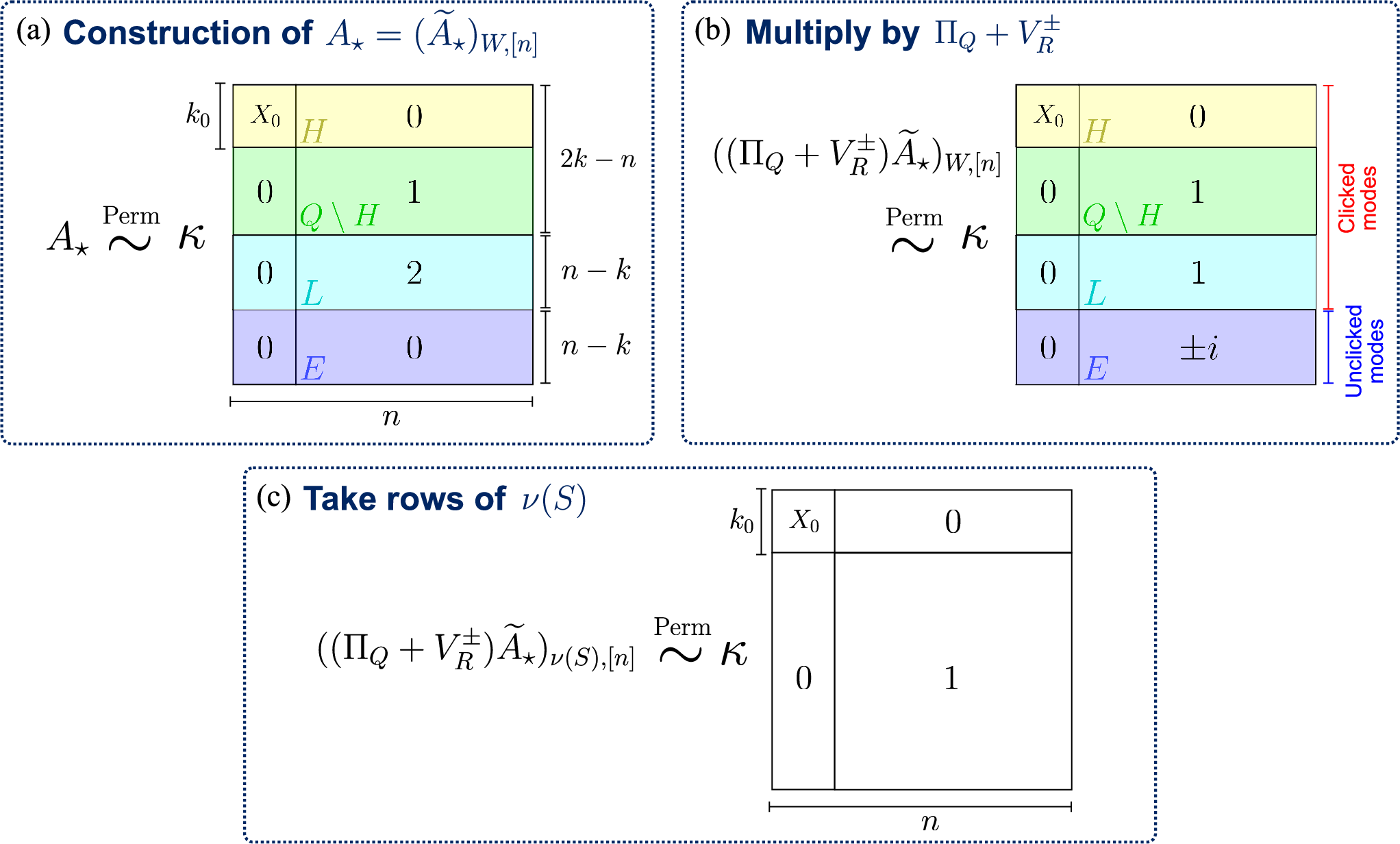
Figure 3: Illustration of the matrix constructions used in the proof of Lemma 4. (a) Schematic of the matrix A⋆=(A~⋆)W,[n]A_{\star}=(\widetilde{A}_{\star})_{W,[n]} in Eq. (48), constructed from a worst-case matrix X0∈{0,1}k0×k0X_{0}\in\{0,1\}^{k_{0}\times k_{0}} with k0<|Q|=2​k−nk_{0}<|Q|=2k-n by adjoining all-zero blocks, an all-ones block, and an all-twos block, together with a normalization factor κ>0\kappa>0. The notation ∼Perm\overset{\mathrm{Perm}}{\sim} denotes equivalence up to row permutations. The row indices corresponding to HH, Q∖HQ\setminus H, LL, and EE are indicated by different colors. (b) Schematic of the matrices ((ΠQ+VR±)​A~⋆)W,[n]((\Pi_{Q}+V_{R}^{\pm})\widetilde{A}_{\star})_{W,[n]} in Eq. (49). (c) Schematic of the matrix ((ΠQ+VR±)​A~⋆)ν⁡(S),[n]((\Pi_{Q}+V_{R}^{\pm})\widetilde{A}_{\star})_{\nu(S),[n]} in Eq. (53), obtained by imposing the constraint supp(S)=supp(x)\supp(S)=\supp(x) and si=1​∀i∈Qs_{i}=1\;\forall i\in Q to (b).
Proof.

We now construct the matrix A⋆A_{\star}; an illustration of the construction is provided in Fig. 3.

We choose an arbitrary subset H⊆QH\subseteq Q of size |H|=k0|H|=k_{0} to encode the hard instance X0X_{0} (see Fig. 3(a)). We define the m×nm\times n completion A~⋆\widetilde{A}_{\star} by specifying the following row blocks, setting all unspecified entries to zero:

(A~⋆)H,{1,…,k0}=κX0,(A~⋆)Q∖H,{k0+1,…,n}=κ1(2​k−n−k0)×(n−k0),(A~⋆)L,{k0+1,…,n}=2​κ​1(n−k)×(n−k0),\displaystyle\begin{split}&(\widetilde{A}_{\star})_{H,\{1,\ldots,k_{0}\}}=\kappa X_{0},\qquad\\ &(\widetilde{A}_{\star})_{Q\setminus H,\{k_{0}+1,\ldots,n\}}=\kappa 1_{(2k-n-k_{0})\times(n-k_{0})},\qquad\\ &(\widetilde{A}_{\star})_{L,\{k_{0}+1,\ldots,n\}}=2\kappa 1_{(n-k)\times(n-k_{0})},\end{split} (48)

where 1a×b1_{a\times b} denotes the a×ba\times b all-one matrix. This construction specifies A⋆=(A~⋆)W,[n]A_{\star}=(\widetilde{A}_{\star})_{W,[n]}.

We next apply the matrix ΠQ+VR±\Pi_{Q}+V_{R}^{\pm} to A~⋆\widetilde{A}_{\star}. The rows indexed by QQ remain unchanged because of the projector ΠQ\Pi_{Q}, whereas the rows indexed by R=L⊔ER=L\sqcup E are transformed according to VR±V_{R}^{\pm} in Eq. (18). Thus, we obtain

((ΠQ+VR±)A~⋆)H,{1,…,k0}=κX0,((ΠQ+VR±)A~⋆)Q∖H,{k0+1,…,n}=κ1(2​k−n−k0)×(n−k0),((ΠQ+VR±)​A~⋆)L,{k0+1,…,n}=κ​1(n−k)×(n−k0)((ΠQ+VR±)​A~⋆)E,{k0+1,…,n}=±i​κ​1(n−k)×(n−k0),\displaystyle\begin{split}&\left((\Pi_{Q}+V_{R}^{\pm})\widetilde{A}_{\star}\right)_{H,\{1,\ldots,k_{0}\}}=\kappa X_{0},\quad\\ &\left((\Pi_{Q}+V_{R}^{\pm})\widetilde{A}_{\star}\right)_{Q\setminus H,\{k_{0}+1,\ldots,n\}}=\kappa 1_{(2k-n-k_{0})\times(n-k_{0})},\quad\\ &\left((\Pi_{Q}+V_{R}^{\pm})\widetilde{A}_{\star}\right)_{L,\{k_{0}+1,\ldots,n\}}=\kappa 1_{(n-k)\times(n-k_{0})}\quad\\ &\left((\Pi_{Q}+V_{R}^{\pm})\widetilde{A}_{\star}\right)_{E,\{k_{0}+1,\ldots,n\}}=\pm i\kappa 1_{(n-k)\times(n-k_{0})},\end{split} (49)

where all unspecified entries are set to zero.

Now consider any SS contributing to Eq. (44); such an SS satisfies supp(S)=O\supp(S)=O and si=1s_{i}=1 for all i∈Qi\in Q. For the modes lj∈Ll_{j}\in L, write

slj=rj,j=1,…,n−k.\displaystyle s_{l_{j}}=r_{j},\qquad j=1,\ldots,n-k. (50)

Because the clicked modes in supp(S)=O=Q⊔L\supp(S)=O=Q\sqcup L have at least one photon, we have rj≥1r_{j}\geq 1 for every jj. Moreover, because the total number of photons outside QQ is N=2​n−2​kN=2n-2k, the occupations satisfy

r1+⋯+rn−k=2​n−2​k.\displaystyle r_{1}+\cdots+r_{n-k}=2n-2k. (51)

For such an SS, the rows indexed by HH appear exactly once and are supported only on the columns indexed by {1,…,k0}\{1,\ldots,k_{0}\}. All other rows appearing in the permanent, namely rows from Q∖HQ\setminus H and repeated rows from LL, are supported only on the columns indexed by {k0+1,…,n}\{k_{0}+1,\ldots,n\} (note that EE rows do not contribute to the permanent). The number of these rows is

|Q∖H|+∑j=1n−krj=(2​k−n−k0)+2​n−2​k=n−k0.\displaystyle|Q\setminus H|+\sum_{j=1}^{n-k}r_{j}=(2k-n-k_{0})+2n-2k=n-k_{0}. (52)

Hence, up to row permutations, the relevant matrix is the block diagonal κ⁡(X0⊕1(n−k0)×(n−k0))\kappa(X_{0}\oplus 1_{(n-k_{0})\times(n-k_{0})}), and thus

Per(((ΠQ+VR±)A~⋆)ν⁡(S),[n])=κnPer(X0)(n−k0)!.\displaystyle\Per\left(\left((\Pi_{Q}+V_{R}^{\pm})\widetilde{A}_{\star}\right)_{\nu(S),[n]}\right)=\kappa^{n}\Per(X_{0})(n-k_{0})!. (53)

We now evaluate the photon-number factorial factor in Eq. (44). Since all modes in QQ contain exactly one photon, they contribute a factor of 11. Hence, the factorial factor depends only on the occupation numbers rjr_{j} in Eq. (50), and is given by

∏isi!=∏j=1n−krj!.\displaystyle\prod_{i}s_{i}!=\prod_{j=1}^{n-k}r_{j}!. (54)

Summing over all r1,…,rn−kr_{1},\ldots,r_{n-k} satisfying Eq. (51) gives exactly the factor Gn,kG_{n,k} in Eq. (47), yielding Eq. (46).

Lastly, one can rewrite Gn,kG_{n,k} by

Gn,k\displaystyle G_{n,k} =[z2​(n−k)]​(ez−1)n−k\displaystyle=[z^{2(n-k)}](e^{z}-1)^{n-k} (55)
=1(2​(n−k))!​∑j=0n−k(−1)n−k−j​(n−kj)​j2​(n−k),\displaystyle=\frac{1}{(2(n-k))!}\sum_{j=0}^{n-k}(-1)^{n-k-j}\binom{n-k}{j}j^{2(n-k)}, (56)

which can be evaluated exactly in polynomial time. ∎

The next lemma shows that the multiplicative factor Gn,kG_{n,k} in Lemma 4 is lower bounded by exp⁡(−O⁡(n))\exp(-O(n)).

Lemma 5.

The multiplicative factor Gn,kG_{n,k} defined in Eq. (47) of Lemma 4 is lower bounded by

Gn,k≥2−n+k=e−O⁡(n).\displaystyle G_{n,k}\geq 2^{-n+k}=e^{-O(n)}. (57)
Proof.

Since all summands in Gn,kG_{n,k} are nonnegative, we may lower bound Gn,kG_{n,k} by restricting the summation to the single occupation pattern

r1=r2=⋯=rn−k=2.\displaystyle r_{1}=r_{2}=\cdots=r_{n-k}=2. (58)

This pattern satisfies r1+⋯+rn−k=2​n−2​kr_{1}+\cdots+r_{n-k}=2n-2k, and contributes

∏j=1n−k12!=2−n+k.\displaystyle\prod_{j=1}^{n-k}\frac{1}{2!}=2^{-n+k}. (59)

Therefore, Gn,k≥2−n+kG_{n,k}\geq 2^{-n+k}. ∎

V.5 Shift-and-scale stability and conditional unitary completion

In the proof of Theorem 1, we interpolate between the hard block A⋆A_{\star} constructed above and a Haar-random unitary submatrix. Let A:=UW,[n]A:=U_{W,[n]} for U∼Haar(m)U\sim\Haar(m), and set A⁡(t):=(1−t)​A+t​A⋆A(t):=(1-t)A+tA_{\star}. We denote by μ\mu the distribution of AA, and by μt\mu_{t} the distribution of A⁡(t)A(t). The following lemma establishes the required shift-and-scale stability bound for square submatrices of Haar-random unitaries.

Lemma 6 (Shift-and-scale stability for TBS).

Let μ\mu be the distribution of A=UW,[n]A=U_{W,[n]} for U∼Haar(m)U\sim\Haar(m) and |W|=n|W|=n, and let μt\mu_{t} be the distribution of A⁡(t)=(1−t)​A+t​A⋆A(t)=(1-t)A+tA_{\star} for A⋆A_{\star} constructed in Lemma 4. Suppose that m−2​n=Ω⁡(n)m-2n=\Omega(n). There exist constants c0,c1,c2>0c_{0},c_{1},c_{2}>0 such that, whenever

0≤t≤c0m​n​(1+κ​n),\displaystyle 0\leq t\leq\frac{c_{0}}{mn(1+\kappa\sqrt{n})}, (60)

the total variation distance between the distributions μ\mu and μt\mu_{t} is bounded by

‖μt−μ‖TVD≤c1​m​n​(1+κ​n)​t+e−c2​(m−2​n).\displaystyle\|\mu_{t}-\mu\|_{\mathrm{TVD}}\leq c_{1}mn(1+\kappa\sqrt{n})t+e^{-c_{2}(m-2n)}. (61)
Proof.

See Appendix H.

∎

The block-level perturbation must also be lifted to the full unitary group, because an instance of the ATE problem in Definition 3 is specified by a complete circuit unitary. To this end, we introduce a conditional unitary-completion procedure that extends the perturbed submatrix to a full unitary while preserving the corresponding total-variation-distance guarantee.

Lemma 7 (Conditional unitary completion for TBS).

Let μ\mu be the distribution of the block A=UW,[n]A=U_{W,[n]} under U∼Haar(m)U\sim\Haar(m), and let μt\mu_{t} be the distribution of the block A⁡(t)=(1−t)​A+t​A⋆A(t)=(1-t)A+tA_{\star}. Suppose that m−2​n=Ω⁡(n)m-2n=\Omega(n) and tt satisfy Eq. (60). There exists a randomized polynomial-time procedure 𝒞\mathcal{C} that, with probability at least 1−exp⁡(−Ω⁡(m−2​n))1-\exp(-\Omega(m-2n)), completes the input matrix to a unitary containing it as the prescribed submatrix. Moreover, the corresponding pushforward measure ℋt:=𝒞#​μt\mathcal{H}_{t}:=\mathcal{C}_{\#}\mu_{t} satisfies

‖ℋt−Haar(m)‖TVD≤‖μt−μ‖TVD+e−Θ⁡(m−2​n).\displaystyle\|\mathcal{H}_{t}-\Haar(m)\|_{\mathrm{TVD}}\leq\|\mu_{t}-\mu\|_{\mathrm{TVD}}+e^{-\Theta(m-2n)}. (62)
Proof.

See Appendix I.

∎

V.6 Application of the extraction procedures

We briefly describe how the two extraction procedures established in Theorems 3 and 4, developed in Secs. IV.2 and IV.3, respectively, are combined to recover the encoded worst-case quantity from average-case estimates of threshold probabilities. Fix a Haar-random block A=UW,[n]A=U_{W,[n]} with U∼Haar(m)U\sim\Haar(m), and let A⋆A_{\star} be the block constructed in Lemma 4. For each sufficiently small t∈[0,Δ]t\in[0,\Delta], where Δ\Delta is specified below, define A⁡(t)=(1−t)​A+t​A⋆A(t)=(1-t)A+tA_{\star}, and let U⁡(t)U(t) be a unitary sampled according to the completion procedure of Lemma 7 applied to A⁡(t)A(t). From estimates of Tx​(VR​(θ)​U​(t))T_{x}(V_{R}(\theta)U(t)), we first estimate the top Fourier coefficient τ2​N​(x,U⁡(t),R)=τ2​Nblk​(x,A⁡(t),R)\tau_{2N}(x,U(t),R)=\tau_{2N}^{\mathrm{blk}}(x,A(t),R) using Theorem 4. Here, the trigonometric degree is at most 2​N≤2​n2N\leq 2n, by Lemma 2. By Eq. (44), the quantity p⁡(t):=τ2​Nblk​(x,A⁡(t),R)p(t):=\tau_{2N}^{\mathrm{blk}}(x,A(t),R) is a polynomial in tt of degree at most 2​n2n, and Lemma 4 shows that its value at t=1t=1 is proportional to Per(X0)2\Per(X_{0})^{2}. The robust Berlekamp–Welch algorithm in Theorem 3 is then applied to the resulting estimates over t∈[0,Δ]t\in[0,\Delta] to recover p⁡(1)=τ2​Nblk​(x,A⋆,R)p(1)=\tau_{2N}^{\mathrm{blk}}(x,A_{\star},R). Thus, the application proceeds as A⁡(t)→U⁡(t)→Tx​(VR​(θ)​U​(t))→τ2​N​(x,U⁡(t),R)→p⁡(t)→p⁡(1)A(t)\to U(t)\to T_{x}(V_{R}(\theta)U(t))\to\tau_{2N}(x,U(t),R)\to p(t)\to p(1), with the error and failure bounds supplied in the proof below.

V.7 Proof of Theorem 1

We are now ready to prove Theorem 1, which establishes the average-case hardness of TBS. More explicitly, we prove the following quantitative statement.

Theorem 5.

Let m=α​nm=\alpha n for a fixed constant α>2\alpha>2. Then ATE problem in Definition 3 is #​P\#\mathrm{P}-hard under a BPPNP\rm{BPP^{NP}} reduction, for additive imprecision

ε≤exp⁡(−3​n​log⁡n−n​log⁡α−O⁡(n)),\displaystyle\varepsilon\leq\exp(-3n\log n - n\log\alpha- O(n)), (63)

and failure probability δ<1/8\delta<1/8.

Proof.

Let 𝒪\mathcal{O} be an oracle for ATE such that, on input x∈𝒯m,nx\in\mathcal{T}_{m,n} and U∈U⁡(m)U\in\mathrm{U}(m), 𝒪\mathcal{O} outputs an estimate satisfying

Prx,U[|𝒪(x,U)−Tx(U)|>εTx(avg)]<δ,\displaystyle\Pr_{x,U}\left[|\mathcal{O}(x,U)-T_{x}(U)|>\varepsilon T_{x}^{(\mathrm{avg})}\right]<\delta, (64)

where the probability is taken over x∼𝒟m,nx\sim\mathcal{D}_{m,n} in Definition 1 and U∼Haar(m)U\sim\Haar(m). We prove that oracle access to 𝒪\mathcal{O} suffices to compute Per(X0)2\Per(X_{0})^{2} exactly for any binary matrix X0∈{0,1}k0×k0X_{0}\in\{0,1\}^{k_{0}\times k_{0}}.

Given X0∈{0,1}k0×k0X_{0}\in\{0,1\}^{k_{0}\times k_{0}}, choose a constant 0<λ<10<\lambda<1 and set n=⌈k01/λ⌉n=\left\lceil k_{0}^{1/\lambda}\right\rceil, so that k0=o⁡(n)k_{0}=o(n). Let m=α​nm=\alpha n for a fixed α>2\alpha>2. We sample x∼𝒟m,nx\sim\mathcal{D}_{m,n} and set k=|x|k=|x|. By Lemma 1, and by choosing η>0\eta>0 small enough so that Eq. (29) holds, the event

|k−αα+1​n|≤η​n\displaystyle\left|k-\frac{\alpha}{\alpha+1}n\right|\leq\eta n (65)

occurs with probability at least 1−exp⁡(−Θ⁡(n))1-\exp(-\Theta(n)). Conditioned on this event, we have k>n/2k>n/2, and both 2​k−n=Θ⁡(n)2k-n=\Theta(n) and n−k=Θ⁡(n)n-k=\Theta(n) hold. In particular, for all sufficiently large nn we have 2​k−n>k02k-n>k_{0}, as required for the construction in Lemma 4.

Conditioned on the event in Eq. (65), let O=supp(x)O=\supp(x), and choose the mode-index sets Q,L,E,RQ,L,E,R, and WW according to Eqs. (30)–(33). Given X0X_{0}, we construct A⋆A_{\star} as in Lemma 4, while keeping κ\kappa unspecified for now. We then sample U∼Haar(m)U\sim\Haar(m), set A:=UW,[n]A:=U_{W,[n]}, define A⁡(t):=(1−t)​A+t​A⋆A(t):=(1-t)A+tA_{\star}, and consider the polynomial

p⁡(t):=τ2​Nblk​(x,A⁡(t),R).\displaystyle p(t):=\tau_{2N}^{\mathrm{blk}}(x,A(t),R). (66)

By Eq. (44), p⁡(t)p(t) is a polynomial in tt of degree at most 2​n2n. Furthermore, Lemma 4 implies

p(1)=κ2​n((n−k0)!)2Gn,kPer(X0)2.\displaystyle p(1)=\kappa^{2n}\left((n-k_{0})!\right)^{2}G_{n,k}\Per(X_{0})^{2}. (67)

We next explain how to estimate p⁡(t)p(t) for a fixed t∈[0,Δ]t\in[0,\Delta]. Given A⁡(t)A(t), we sample a unitary U⁡(t)∈U⁡(m)U(t)\in\mathrm{U}(m) satisfying

U​(t)W,[n]=A⁡(t)\displaystyle U(t)_{W,[n]}=A(t) (68)

by the completion procedure in Lemma 7, which succeeds with probability at least 1−exp⁡(−Ω⁡(n))1-\exp(-\Omega(n)). Let ℋt\mathcal{H}_{t} denote the distribution of the completed unitary.

Choose Δ:=cδ/m​n​(1+κ​n)\Delta:={c_{\delta}}/{mn(1+\kappa\sqrt{n})} for a sufficiently small constant cδ>0c_{\delta}>0. Since m−2​n=(α−2)​n=Ω⁡(n)m-2n=(\alpha-2)n=\Omega(n), Lemma 6 and Lemma 7 imply that, for every t∈[0,Δ]t\in[0,\Delta],

‖ℋt−Haar(m)‖TVD≤1/8−δ2+e−Θ⁡(n).\displaystyle\|\mathcal{H}_{t}-\Haar(m)\|_{\mathrm{TVD}}\leq\frac{1/8-\delta}{2}+e^{-\Theta(n)}. (69)

Combining all the preceding arguments, for all sufficiently large nn, the failure probability for estimating Tx​(U​(t))T_{x}(U(t)) with additive imprecision at most ε​Tx(avg)\varepsilon T_{x}^{(\mathrm{avg})} is bounded by

δ+e−Θ⁡(n)+e−Ω⁡(n)+1/8−δ2+e−Θ⁡(n)<18.\displaystyle\delta+e^{-\Theta(n)}+e^{-\Omega(n)}+\frac{1/8-\delta}{2}+e^{-\Theta(n)}<\frac{1}{8}. (70)

Here, δ\delta is the oracle failure probability in Eq. (64), the first exponentially small term is the failure probability of the typical event in Eq. (65), and the second is the failure probability of the completion procedure associated with Eq. (68). The last two terms are respectively the block-to-Haar total variation contribution and the boundary contribution in Eq. (69). Therefore, for all sufficiently large nn,

Pr[|𝒪(x,U(t))−Tx(U(t))|>εTx(avg)]<18.\displaystyle\Pr\left[|\mathcal{O}(x,U(t))-T_{x}(U(t))|>\varepsilon T_{x}^{(\mathrm{avg})}\right]<\frac{1}{8}. (71)

The same bound also holds with U⁡(t)U(t) replaced by VR​(θ)​U​(t)V_{R}(\theta)U(t) for any fixed θ\theta, since left multiplication by VR​(θ)V_{R}(\theta) preserves Haar measure and does not increase total variation distance from Haar.

We now apply the robust Fourier coefficient extraction algorithm. Since Tx​(VR​(θ)​U​(t))T_{x}(V_{R}(\theta)U(t)) is a trigonometric polynomial with degree at most 2​N≤2​n2N\leq 2n, Theorem 4 yields an estimate p^​(t)\widehat{p}(t) satisfying

Pr[|p^(t)−p(t)|>εTx(avg)eO⁡(n)]<14.\displaystyle\Pr\left[|\widehat{p}(t)-p(t)|>\varepsilon T_{x}^{(\mathrm{avg})}e^{O(n)}\right]<\frac{1}{4}. (72)

We repeat this procedure at the interpolation points tj∈[0,Δ]t_{j}\in[0,\Delta] specified in Theorem 3. The robust Berlekamp–Welch algorithm then yields an estimate p^​(1)\widehat{p}(1) satisfying

Pr[|p^(1)−p(1)|>εTx(avg)exp⁡(2​n​log⁡Δ−1+O⁡(n))]<13.\displaystyle\Pr\left[|\widehat{p}(1)-p(1)|>\varepsilon T_{x}^{(\mathrm{avg})}\exp(2n\log\Delta^{-1}+O(n))\right]<\frac{1}{3}. (73)

Using Eq. (67), we divide the obtained estimate p^​(1)\widehat{p}(1) by the known factor κ2​n​((n−k0)!)2​Gn,k\kappa^{2n}((n-k_{0})!)^{2}G_{n,k} to obtain an estimate of Per(X0)2\Per(X_{0})^{2} within additive imprecision

ε′:=ε​Tx(avg)​exp⁡(2​n​log⁡Δ−1+O⁡(n))κ2​n​((n−k0)!)2​Gn,k.\displaystyle\varepsilon^{\prime}:=\frac{\varepsilon T_{x}^{(\mathrm{avg})}\exp(2n\log\Delta^{-1}+O(n))}{\kappa^{2n}\left((n-k_{0})!\right)^{2}G_{n,k}}. (74)

It remains only to bound the above quantity. We now choose κ=1/n\kappa=1/\sqrt{n}, so that κ−2​n=nn=exp⁡(n​log⁡n)\kappa^{-2n}=n^{n}=\exp(n\log n). Also, by definition, we have Δ−1=O⁡(α​n2)\Delta^{-1}=O(\alpha n^{2}), and hence

exp⁡(2​n​log⁡Δ−1)≤exp⁡(4​n​log⁡n+2​n​log⁡α+O⁡(n)).\displaystyle\exp(2n\log\Delta^{-1})\leq\exp(4n\log n+2n\log\alpha+O(n)). (75)

Since k0=O⁡(nλ)k_{0}=O(n^{\lambda}) with λ<1\lambda<1, Stirling’s formula gives

((n−k0)!)2=exp⁡(2​n​log⁡n−O⁡(n)).\displaystyle\left((n-k_{0})!\right)^{2}=\exp(2n\log n-O(n)). (76)

By Lemma 5, we have Gn,k−1=eO⁡(n)G_{n,k}^{-1}=e^{O(n)}. Finally, for fixed α>2\alpha>2, Lemma 15 in Appendix B gives

Tx(avg)≤exp⁡(−n​log⁡α+O⁡(n)).\displaystyle T_{x}^{(\mathrm{avg})}\leq\exp(-n\log\alpha+O(n)). (77)

Substituting Eq. (75)–Eq. (77) into Eq. (74), we obtain

ε′\displaystyle\varepsilon^{\prime} ≤ε​exp⁡(3​n​log⁡n+n​log⁡α+O⁡(n)).\displaystyle\leq\varepsilon\exp(3n\log n+n\log\alpha+O(n)). (78)

Therefore, if

ε≤exp⁡(−3​n​log⁡n−n​log⁡α−O⁡(n)),\displaystyle\varepsilon\leq\exp(-3n\log n- n\log\alpha-O(n)), (79)

then the constant hidden in O⁡(n)O(n) can be chosen so that ε′<1/2\varepsilon^{\prime}<1/2. Rounding the resulting estimate to the nearest integer therefore yields Per(X0)2\Per(X_{0})^{2} exactly. Moreover, the overall procedure succeeds with probability at least 2/32/3, and repetition and majority voting can arbitrarily boost this success probability. All steps of the reduction are polynomial-time procedures with access to an NP oracle. Therefore, oracle access to ATE with ε\varepsilon satisfying Eq. (79) and failure probability δ<1/8\delta<1/8 allows the exact computation of Per(X0)2\Per(X_{0})^{2} for arbitrary X0∈{0,1}k0×k0X_{0}\in\{0,1\}^{k_{0}\times k_{0}}, where the overall procedure is in BPPNP\rm{BPP^{NP}}.

∎

VI Parity BosonSampling

We now prove Theorem 2. The proof follows the common worst-to-average-case reduction described in Sec. III.3, while retaining the parity-specific beam-splitter rotations and permanent-encoding construction, illustrated in Fig. 4.

VI.1 Proof overview

Refer to caption
Figure 4: Parity-specific Fourier-filtering construction used in the proof of Theorem 2. Starting from a sampled parity outcome x∼𝒴m,nx\sim\mathcal{Y}_{m,n} with |x|=k|x|=k odd parities, we choose kk even-parity modes and apply paired beam-splitter rotations B⁡(θ)B(\theta) to all odd-even pairs. The resulting probability becomes a Fourier series in θ\theta of degree at most 2​n2n. Its top Fourier coefficient, denoted by c2​nc_{2n}, filters out all contributions except those in which all nn photons occupy the rotated modes, and therefore depends only on the corresponding 2​k×n2k\times n submatrix UR,[n]U_{R,[n]}. The shared worst-to-average-case reduction procedure is described in Secs. III.3 and IV.

We provide an overview of the worst-to-average-case reduction proving Theorem 2. As in the TBS case, the reduction starts from an arbitrary k0×k0k_{0}\times k_{0} binary matrix X0X_{0} and shows that oracle access to APE in Definition 4 enables the exact computation of Per(X0)2\Per(X_{0})^{2}. Since exact computation of the permanent of a binary matrix is #P-hard in the worst case [37], this establishes the desired hardness result.

We first establish a typical-outcome property for the parity ensemble. For x∼𝒴m,nx\sim\mathcal{Y}_{m,n} with m=α​nm=\alpha n, Lemma 8 shows that the number of odd-parity modes concentrates near α​n/(α+2)\alpha n/(\alpha+2). Writing k=|x|k=|x| and O=supp(x)O=\supp(x), a typical outcome therefore has k=Θ⁡(n)k=\Theta(n) odd-parity modes. We then choose a set E⊆[m]∖OE\subseteq[m]\setminus O of kk even-parity modes and fix a pairing between the modes in OO and those in EE. Denoting the union of these paired modes by R:=O⊔ER:=O\sqcup E, we have |R|=2​k|R|=2k. For fixed α>2\alpha>2, the same typical-outcome event also guarantees the margin m−n−2​k=Ω⁡(n)m-n-2k=\Omega(n) required later for the Haar-submatrix perturbation argument.

For these fixed mode sets, consider an arbitrary linear-optical circuit UU. We apply identical coherent beam-splitter rotations to all paired modes in RR and examine the resulting parity probability Px​(VR​(θ)​U)P_{x}(V_{R}(\theta)U) as a function of the rotation angle θ\theta. This probability is a finite Fourier series of degree at most 2​n2n. Unlike in the threshold setting, however, the original parity probability is not determined by UR,[n]U_{R,[n]}: modes outside RR have even parity and may still contain a positive even number of photons, so Px​(U)P_{x}(U) generally depends on the full m×nm\times n input-output block. The crucial role of the highest-order Fourier coefficient c2​nc_{2n} is to remove this global dependence. To contribute at frequency 2​n2n, all nn photons must occupy the rotated modes in RR. Consequently, c2​nc_{2n} depends only on the rectangular block UR,[n]U_{R,[n]} (Lemma 10), providing the localized block into which the worst-case instance can be encoded.

In Lemma 11, we use this localization to encode the worst-case instance X0X_{0}. Choose k0k_{0} of the odd-parity modes to carry the rows of X0X_{0}. We construct a 2​k×n2k\times n block A⋆A_{\star} that embeds X0X_{0} on these selected odd-mode rows, while its other entries are chosen so that every nonvanishing contribution to the top Fourier coefficient contains each hard row exactly once. For every surviving occupation pattern, the corresponding permanent reduces, up to known phase factors, to κnPer(X0)(n−k0)!\kappa^{n}\Per(X_{0})(n-k_{0})!, with these phases canceling between the two permanent factors in the top Fourier coefficient. Lastly, summing over the remaining occupation patterns contributes only the explicitly known and efficiently computable factor Qn,k,k0Q_{n,k,k_{0}}. Thus, the resulting top Fourier coefficient is proportional to Per(X0)2\Per(X_{0})^{2} with known prefactor κ2​n​((n−k0)!)2​Qn,k,k0\kappa^{2n}((n-k_{0})!)^{2}Q_{n,k,k_{0}} (Lemma 11). The condition k0<kk_{0}<k required by the construction holds for the chosen k0=o⁡(n)k_{0}=o(n) and for typical x∼𝒴m,nx\sim\mathcal{Y}_{m,n}.

The remainder of the reduction then follows the common workflow in Sec. III.3 and invokes the technical results established in Sec. IV. Lemma 13 bounds the distributional change induced by the affine block perturbation, and Lemma 14 lifts this perturbation to a full unitary through conditional completion. Finally, Theorem 4 extracts the relevant Fourier coefficient from APE estimates, and Theorem 3 extrapolates this coefficient to the endpoint encoding the worst-case quantity.

The rest of this section proceeds as follows. In Sec. VI.2, we show that most parity outcomes have the number of odd parities concentrated near α​n/(α+2)\alpha n/(\alpha+2). In Sec. VI.3, we introduce the parity Fourier coefficients, establish their band limitation, and derive the top-coefficient row filter. In Sec. VI.4, we show how to encode the worst-case #P-hard quantity into the parity Fourier coefficient for most parity outcomes. In Sec. VI.5, we specialize the shift-and-scale stability and unitary-completion framework to the parity setting. Finally, in Sec. VI.6, we complete the proof of Theorem 2.

VI.2 Odd-parity count concentration

We first show that, for x∼𝒴m,nx\sim\mathcal{Y}_{m,n}, the number of odd-parity modes |x||x| concentrates near α​n/(α+2)\alpha n/(\alpha+2).

Lemma 8 (Odd-parity concentration).

Let α=m/n≥1\alpha=m/n\geq 1, and fix η∈(0,min⁡{α/(α+2),2/(α+2)})\eta\in(0,\min\left\{\alpha/(\alpha+2),2/(\alpha+2)\right\}). Let 𝒴m,n\mathcal{Y}_{m,n} be the distribution in Definition 2. Then, for all sufficiently large nn, there exist constants Cα,η,cα,η>0C_{\alpha,\eta},c_{\alpha,\eta}>0 such that

Prx∼𝒴m,n[||x|−αα+2n|≥ηn]≤Cα,ηe−cα,η​n\displaystyle\Pr_{x\sim\mathcal{Y}_{m,n}}\left[\left||x|-\frac{\alpha}{\alpha+2}n\right|\geq\eta n\right]\leq C_{\alpha,\eta}e^{-c_{\alpha,\eta}n} (80)
Proof.

See Appendix C. ∎

Lemma 8 implies that, for x∼𝒴m,nx\sim\mathcal{Y}_{m,n}, the event |x|=Θ⁡(n)|x|=\Theta(n) occurs with probability at least 1−exp⁡(−Θ⁡(n))1-\exp(-\Theta(n)). Moreover, for any fixed α>2\alpha>2, choosing a sufficiently small η>0\eta>0 yields

m−n−2​|x|\displaystyle m-n-2|x| ≥(α−1−2​αα+2−2​η)​n=Ω⁡(n),\displaystyle\geq\left(\alpha-1-\frac{2\alpha}{\alpha+2}-2\eta\right)n=\Omega(n), (81)

again with probability at least 1−exp⁡(−Θ⁡(n))1-\exp(-\Theta(n)). These two properties are the typical-outcome inputs exploited in the proof of Theorem 2.

VI.3 Parity Fourier coefficients and band limitation

Using the paired beam-splitter rotations defined in Sec. IV.1, we now define the Fourier coefficients of the parity probability as a function of the rotation angle. Let R⊆[m]R\subseteq[m] be a paired active set as defined in Sec. IV.1.

Definition 6 (Fourier coefficient).

Given x∈𝒫m,nx\in\mathcal{P}_{m,n}, U∈U⁡(m)U\in\mathrm{U}(m), and a paired active set RR as above, define

cℓ​(x,U,R):=12​π​∫02​πPx​(VR​(θ)​U)​e−i​ℓ​θ​𝑑θ,ℓ∈ℤ.\displaystyle c_{\ell}(x,U,R):=\frac{1}{2\pi}\int_{0}^{2\pi}P_{x}(V_{R}(\theta)U)e^{-i\ell\theta}\,d\theta,\quad\ell\in\mathbb{Z}. (82)

We next show that this function of θ\theta is band-limited, such that its Fourier support lies in {−2​n,…,2​n}\{-2n,\ldots,2n\}.

Lemma 9.

For any fixed x∈𝒫m,nx\in\mathcal{P}_{m,n}, U∈U⁡(m)U\in\mathrm{U}(m), and paired active set RR, the parity output probability Px​(VR​(θ)​U)P_{x}(V_{R}(\theta)U) is a trigonometric polynomial in θ\theta of degree at most 2​n2n. Equivalently,

Px​(VR​(θ)​U)=∑ℓ=−2​n2​ncℓ​(x,U,R)​ei​ℓ​θ,\displaystyle P_{x}(V_{R}(\theta)U)=\sum_{\ell=-2n}^{2n}c_{\ell}(x,U,R)e^{i\ell\theta}, (83)

where the coefficients are given in Definition 6.

Proof.

Write UR​(θ):=VR​(θ)​UU_{R}(\theta):=V_{R}(\theta)U throughout the proof. For a fixed S∈𝒮m,nS\in\mathcal{S}_{m,n}, let nR​(S):=∑i∈Rsin_{R}(S):=\sum_{i\in R}s_{i} be the number of photons detected in the output modes indexed by RR. By Eq. (21), the submatrix UR​(θ)ν⁡(S),[n]U_{R}(\theta)_{\nu(S),[n]} contains exactly nR​(S)n_{R}(S) θ\theta-dependent rows, counted with multiplicity, while all other rows are independent of θ\theta. By the row multilinearity of the permanent established in Sec. IV.1, Per(UR​(θ)ν⁡(S),[n])\Per(U_{R}(\theta)_{\nu(S),[n]}) has degree at most nR​(S)n_{R}(S) in e±i​θe^{\pm i\theta}. Consequently, its squared modulus is a trigonometric polynomial of degree at most 2​nR​(S)2n_{R}(S). Summing over SS as in Eq. (9) preserves this bound, and since nR​(S)≤nn_{R}(S)\leq n, the parity probability Px​(UR​(θ))P_{x}(U_{R}(\theta)) is a trigonometric polynomial in θ\theta of degree at most 2​n2n.

∎

Now fix α=m/n>2\alpha=m/n>2 and a parity string x∈𝒫m,nx\in\mathcal{P}_{m,n} with weight |x|=k|x|=k. In the reduction we will restrict to typical outcomes for which k=Θ⁡(n)k=\Theta(n) and m−n−2​k=Ω⁡(n)m-n-2k=\Omega(n). By Lemma 8, these conditions hold with probability at least 1−exp⁡(−Θ⁡(n))1-\exp(-\Theta(n)) when x∼𝒴m,nx\sim\mathcal{Y}_{m,n}.

For the fixed xx, let O:=supp(x)O:=\supp(x) be the set of odd-parity modes; thus |O|=k|O|=k. Choose an arbitrary set E⊆[m]∖OE\subseteq[m]\setminus O with |E|=k|E|=k, and fix a perfect matching between OO and EE:

R:=O⊔E={o1,e1}⊔⋯⊔{ok,ek},\displaystyle R:=O\sqcup E=\{o_{1},e_{1}\}\sqcup\cdots\sqcup\{o_{k},e_{k}\}, (84)

where oj∈Oo_{j}\in O and ej∈Ee_{j}\in E. We regard this pairing as part of the data defining RR.

Applying the beam-splitter rotation VR​(θ)V_{R}(\theta) to these paired output modes gives the Fourier coefficients cℓ​(x,U,R)c_{\ell}(x,U,R) from Definition 6. We focus on the highest-frequency coefficient

c2​n​(x,U,R)=12​π​∫02​πPx​(VR​(θ)​U)​e−i​2​n​θ​𝑑θ,\displaystyle c_{2n}(x,U,R)=\frac{1}{2\pi}\int_{0}^{2\pi}P_{x}(V_{R}(\theta)U)e^{-i2n\theta}\,d\theta, (85)

which we also refer to as the top Fourier coefficient.

Importantly, while Px​(U)P_{x}(U) itself depends on the entire m×nm\times n block of UU (first nn columns), the top coefficient depends only on a 2​k×n2k\times n submatrix of UU, as shown in the following lemma.

Lemma 10.

Let x∈𝒫m,nx\in\mathcal{P}_{m,n}, U∈U⁡(m)U\in{\rm U}(m), and R=O⊔ER=O\sqcup E for O=supp(x)O=\supp(x) and any choice of E⊆[m]∖OE\subseteq[m]\setminus O with |E|=|O||E|=|O|. Then only configurations satisfying nR​(S):=∑i∈Rsi=nn_{R}(S):=\sum_{i\in R}s_{i}=n, equivalently supp(S)⊆R\supp(S)\subseteq R, contribute to the top Fourier coefficient, and

c2​n​(x,U,R)\displaystyle c_{2n}(x,U,R)
=∑S∈𝒮m,nS​mod​ 2=xnR​(S)=n1∏isi!Per((VR+U)ν⁡(S),[n])Per((VR−U)ν⁡(S),[n])∗.\displaystyle=\!\!\!\!\!\sum_{\begin{subarray}{c}S\in\mathcal{S}_{m,n}\\ S\;{\rm mod}\;2=x\\ n_{R}(S)=n\end{subarray}}\!\!\!\!\!\frac{1}{\prod_{i}s_{i}!}\,\Per\!\big((V_{R}^{+}U)_{\nu(S),[n]}\big)\Per\!\big((V_{R}^{-}U)_{\nu(S),[n]}\big)^{*}. (86)

Moreover, since VR±V_{R}^{\pm} has support only on rows indexed by RR, the coefficient c2​n​(x,U,R)c_{2n}(x,U,R) depends only on the 2​k×n2k\times n submatrix UR,[n]U_{R,[n]} of UU.

This isolation property plays a central role in the hardness proof, particularly in the PBS setting, because it allows us to apply perturbation-stability results for Haar-random submatrices when embedding the worst-case matrix as a small perturbation, as in related constructions [3, 4, 5, 11, 12, 31].

Proof of Lemma 10.

As in the proof of Lemma 9, we denote UR​(θ)=VR​(θ)​UU_{R}(\theta)=V_{R}(\theta)U throughout this proof. By definition, the top coefficient can be expressed as

c2​n​(x,U,R)\displaystyle c_{2n}(x,U,R)
=∑S∈𝒮m,nS​mod 2=x1∏isi!⋅12​π∫02​π|Per(UR(θ)ν⁡(S),[n])|2e−i2n​θdθ.\displaystyle=\!\!\!\!\!\!\sum_{\begin{subarray}{c}S\in\mathcal{S}_{m,n}\\ S\;\text{mod 2}=x\end{subarray}}\!\!\!\!\frac{1}{\prod_{i}s_{i}!}\cdot\frac{1}{2\pi}\int_{0}^{2\pi}\Big|\Per\big(U_{R}(\theta)_{\nu(S),[n]}\big)\Big|^{2}\,e^{-i2n\theta}\,d\theta. (87)

For a given S∈𝒮m,nS\in\mathcal{S}_{m,n}, let nR​(S):=∑i∈Rsin_{R}(S):=\sum_{i\in R}s_{i} be the number of photons occupying the output modes RR. As argued in the proof of Lemma 9, Eq. (21) and multilinearity of permanent implies that |Per(UR​(θ)ν⁡(S),[n])|2\big|\Per(U_{R}(\theta)_{\nu(S),[n]})\big|^{2} is a trigonometric polynomial in θ\theta of degree at most 2​nR​(S)2n_{R}(S). Therefore, the integrand in Eq. (87) contains no ei​2​n​θe^{i2n\theta} term unless 2​nR​(S)≥2​n2n_{R}(S)\geq 2n, which, by constraint nR​(S)≤nn_{R}(S)\leq n, forces nR​(S)=nn_{R}(S)=n. Accordingly, for every SS contributing to c2​n​(x,U,R)c_{2n}(x,U,R), all photons must occupy the modes confined in RR, and for such SS, every row of UR​(θ)ν⁡(S),[n]U_{R}(\theta)_{\nu(S),[n]} has the form:

(UR​(θ)ν⁡(S),[n])j\displaystyle(U_{R}(\theta)_{\nu(S),[n]})_{j} =ei​θ​((VR+​U)ν⁡(S),[n])j\displaystyle=e^{i\theta}\,((V_{R}^{+}U)_{\nu(S),[n]})_{j}
+e−i​θ​((VR−​U)ν⁡(S),[n])j.\displaystyle+e^{-i\theta}\,((V_{R}^{-}U)_{\nu(S),[n]})_{j}. (88)

By multilinearity over the nn rows, expanding Per(UR​(θ)ν⁡(S),[n])\Per(U_{R}(\theta)_{\nu(S),[n]}) yields a sum of 2n2^{n} terms, one for each choice of whether to pick the ei​θe^{i\theta} or e−i​θe^{-i\theta} part in each row. Here, the largest exponent ei​n​θe^{in\theta} occurs when we pick the ei​θe^{i\theta} part from every row, and the corresponding coefficient is exactly Per((VR+​U)ν⁡(S),[n])\Per\big((V_{R}^{+}U)_{\nu(S),[n]}\big). Similarly, the smallest exponent e−i​n​θe^{-in\theta} occurs when we pick the e−i​θe^{-i\theta} part from every row, and its coefficient is Per((VR−​U)ν⁡(S),[n])\Per\big((V_{R}^{-}U)_{\nu(S),[n]}\big). Therefore, the coefficient of ei​2​n​θe^{i2n\theta} in |Per(UR​(θ)ν⁡(S),[n])|2\big|\Per(U_{R}(\theta)_{\nu(S),[n]})\big|^{2} is given by

Per((VR+​U)ν⁡(S),[n])⋅Per((VR−​U)ν⁡(S),[n])∗.\displaystyle\Per\big((V_{R}^{+}U)_{\nu(S),[n]}\big)\cdot{\Per\big((V_{R}^{-}U)_{\nu(S),[n]}\big)}^{*}. (89)

Since the integration over θ\theta in Eq. (87) extracts exactly the coefficient of ei​2​n​θe^{i2n\theta} by the orthogonality, this yields Eq. (86).

∎

VI.4 Encoding a single permanent into the parity Fourier coefficient

Similarly to the threshold case, we generalize the definition of the top Fourier coefficient to take a rectangular matrix A∈ℂ2​k×nA\in\mathbb{C}^{2k\times n} as an input, instead of a unitary matrix. To this end, we use a convention A~∈ℂm×n\widetilde{A}\in\mathbb{C}^{m\times n} to denote any matrix completion of AA that satisfies A~R,[n]=A\widetilde{A}_{R,[n]}=A. This allows us to define the block extension of the top Fourier coefficient in Lemma 10 by

c2​nblk​(x,A,R)\displaystyle c^{\mathrm{blk}}_{2n}(x,A,R)
:=∑S∈𝒮m,nSmod2=x1∏isi!Per((VR+A~)ν⁡(S),[n])Per((VR−A~)ν⁡(S),[n])∗.\displaystyle:=\!\!\!\!\!\sum_{\begin{subarray}{c}S\in\mathcal{S}_{m,n}\\ S\bmod 2=x\end{subarray}}\!\!\!\!\frac{1}{\prod_{i}s_{i}!}\Per\left((V_{R}^{+}\widetilde{A})_{\nu(S),[n]}\right)\Per\left((V_{R}^{-}\widetilde{A})_{\nu(S),[n]}\right)^{*}. (90)

Accordingly, by Lemma 10, whenever A=UR,[n]A=U_{R,[n]} for a unitary UU, we have

c2​nblk​(x,UR,[n],R)=c2​n​(x,U,R).\displaystyle c^{\mathrm{blk}}_{2n}(x,U_{R,[n]},R)=c_{2n}(x,U,R). (91)

We now describe how to encode a worst-case #P-hard quantity into this top Fourier coefficient. Specifically, let X0∈{0,1}k0×k0X_{0}\in\{0,1\}^{k_{0}\times k_{0}} be an arbitrary worst-case instance, with k0=o⁡(n)k_{0}=o(n) in the reduction. In the following lemma, we construct a 2​k×n2k\times n worst-case matrix A⋆∈ℂ2​k×nA_{\star}\in\mathbb{C}^{2k\times n} such that c2​nblk​(x,A⋆,R)c^{\mathrm{blk}}_{2n}(x,A_{\star},R) encodes Per(X0)2\Per(X_{0})^{2} up to a known multiplicative factor, so that estimating c2​nblk​(x,A⋆,R)c^{\mathrm{blk}}_{2n}(x,A_{\star},R) immediately yields an estimate of Per(X0)2\Per(X_{0})^{2}.

Lemma 11 (Single-permanent encoding).

Fix α=m/n>2\alpha=m/n>2. Let x∈𝒫m,nx\in\mathcal{P}_{m,n} with |x|=k|x|=k, and let R=O⊔ER=O\sqcup E for O=supp(x)O=\supp(x) and any choice of E⊆[m]∖OE\subseteq[m]\setminus O with |E|=|O||E|=|O|. Let c2​nblkc^{\mathrm{blk}}_{2n} be the block extension of the top Fourier coefficient in Eq. (90). Given a matrix X0∈{0,1}k0×k0X_{0}\in\{0,1\}^{k_{0}\times k_{0}} with k0<kk_{0}<k, there exists a 2​k×n2k\times n matrix A⋆∈ℂ2​k×nA_{\star}\in\mathbb{C}^{2k\times n} that can be constructed in polynomial time and satisfies

c2​nblk(x,A⋆,R)=κ2​n((n−k0)!)2Qn,k,k0Per(X0)2,\displaystyle c^{\mathrm{blk}}_{2n}(x,A_{\star},R)=\kappa^{2n}\left((n-k_{0})!\right)^{2}Q_{n,k,k_{0}}\Per(X_{0})^{2}, (92)

where κ>0\kappa>0 is a free normalization parameter one can arbitrarily choose, and the factor

Qn,k,k0:=∑a1,…,ak−k0≥0b1,…,bk−k0≥0∑j=1k−k0((2​aj+1)+2​bj)=n−k0∏j=1k−k01(2​aj+1)!​(2​bj)!,\displaystyle Q_{n,k,k_{0}}:=\!\!\!\!\!\!\!\!\!\!\sum_{\begin{subarray}{c}a_{1},\ldots,a_{k-k_{0}}\geq 0\\ b_{1},\ldots,b_{k-k_{0}}\geq 0\\ \sum_{j=1}^{k-k_{0}}\left((2a_{j}+1)+2b_{j}\right)=n-k_{0}\end{subarray}}\!\!\!\!\!\!\!\!\!\prod_{j=1}^{k-k_{0}}\frac{1}{(2a_{j}+1)!(2b_{j})!}, (93)

which can be computed in polynomial time.
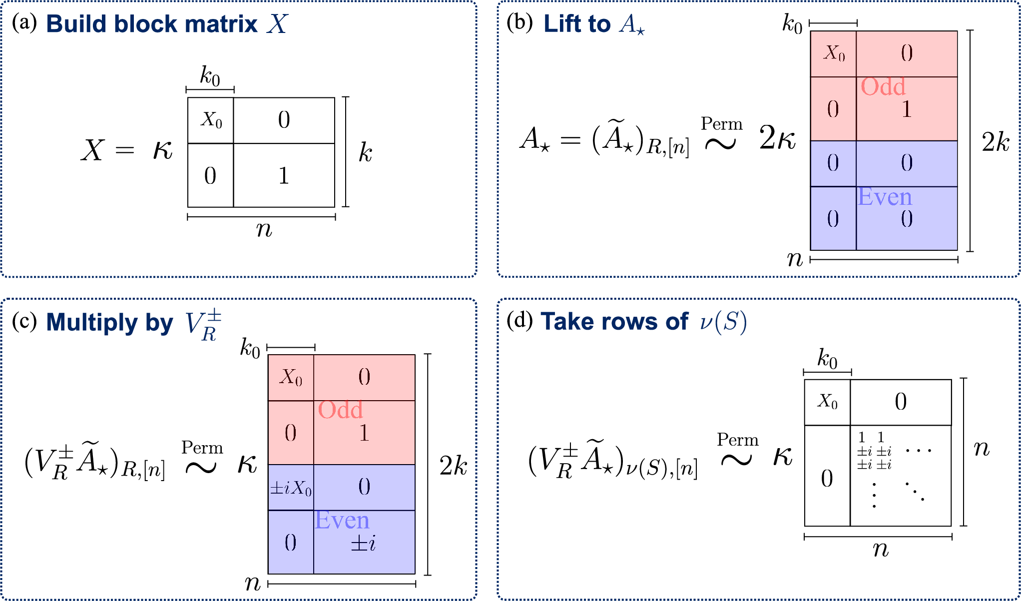
Refer to caption
Figure 5: Illustration of the matrix constructions in the proof of Lemma 11. (a) Schematic of the block matrix XX in Eq. (94), constructed from a worst-case matrix X0∈{0,1}k0×k0X_{0}\in\{0,1\}^{k_{0}\times k_{0}} (where k0<kk_{0}<k) by adjoining all-zero blocks and an all-ones block, together with a normalization factor κ>0\kappa>0. (b) Schematic of the matrix A⋆=(A~⋆)R,[n]A_{\star}=(\widetilde{A}_{\star})_{R,[n]} in Eq. (95), obtained by embedding XX into the rows indexed by R=O⊔ER=O\sqcup E and the first nn columns of a larger matrix A~⋆\widetilde{A}_{\star}. In the figure, the labels “odd” and “even” inside the blocks indicate the rows indexed by OO and EE, respectively, corresponding to the modes where odd and even parities are measured. The notation ∼Perm\overset{\mathrm{Perm}}{\sim} denotes equivalence up to row permutations. (c) Schematic of the matrices (VR±​A~⋆)R,[n](V_{R}^{\pm}\widetilde{A}_{\star})_{R,[n]} in Eq. (96). (d) Schematic of the matrix (VR±​A~⋆)ν⁡(S),[n](V_{R}^{\pm}\widetilde{A}_{\star})_{\nu(S),[n]} used in Eq. (97), obtained from (c) after imposing the constraint Smod2=xS\bmod 2=x.
Proof.

We construct the matrix A⋆A_{\star} below; an illustration of the construction is provided in Fig. 5.

Given a matrix X0∈{0,1}k0×k0X_{0}\in\{0,1\}^{k_{0}\times k_{0}}, define the k×nk\times n matrix

X:=κ​(X00k0×(n−k0)0(k−k0)×k01(k−k0)×(n−k0)),\displaystyle X:=\kappa\begin{pmatrix}X_{0}&0_{k_{0}\times(n-k_{0})}\\ 0_{(k-k_{0})\times k_{0}}&1_{(k-k_{0})\times(n-k_{0})}\end{pmatrix}, (94)

where κ\kappa is a free parameter one can arbitrarily choose, and 0a×b0_{a\times b} and 1a×b1_{a\times b} denote the a×ba\times b all-zero and all-one matrices, respectively. Provided that R=O⊔ER=O\sqcup E for odd and even modes OO and EE, one can construct a matrix A⋆∈ℂ2​k×nA_{\star}\in\mathbb{C}^{2k\times n} whose m×nm\times n completion A~⋆\widetilde{A}_{\star} satisfies

(A~⋆)O,[n]=2​X,(A~⋆)E,[n]=0.\displaystyle(\widetilde{A}_{\star})_{O,[n]}=2X,\quad(\widetilde{A}_{\star})_{E,[n]}=0. (95)

By Eq. (18), this also gives

(VR±​A~⋆)O,[n]=X,(VR±​A~⋆)E,[n]=±i​X.\displaystyle(V_{R}^{\pm}\widetilde{A}_{\star})_{O,[n]}=X,\quad(V_{R}^{\pm}\widetilde{A}_{\star})_{E,[n]}=\pm iX. (96)

Based on this construction, consider the corresponding top Fourier coefficient:

c2​nblk​(x,A⋆,R)\displaystyle c^{\mathrm{blk}}_{2n}(x,A_{\star},R) =∑S∈𝒮m,nSmod2=x1∏isi!Per((VR+A~⋆)ν⁡(S),[n])\displaystyle=\!\!\!\!\!\!\sum_{\begin{subarray}{c}S\in\mathcal{S}_{m,n}\\ S\bmod 2=x\end{subarray}}\!\!\!\!\!\frac{1}{\prod_{i}s_{i}!}\Per\left((V_{R}^{+}\widetilde{A}_{\star})_{\nu(S),[n]}\right)
×Per((VR−​A~⋆)ν⁡(S),[n])∗.\displaystyle\qquad\qquad\qquad\times\Per\left((V_{R}^{-}\widetilde{A}_{\star})_{\nu(S),[n]}\right)^{*}. (97)

Recall that oj∈Oo_{j}\in O and ej∈Ee_{j}\in E denote the odd and even mode indices, respectively. By the block-diagonal structure of XX in Eq. (94), for each j=1,…,k0j=1,\ldots,k_{0}, the rows of VR±​A~⋆V_{R}^{\pm}\widetilde{A}_{\star} indexed by ojo_{j} and eje_{j} are supported on the first k0k_{0} columns. The parity constraint forces each hard odd mode ojo_{j} to contain at least one photon. If any additional photon occupied one of the hard pairs, then the corresponding matrix would contain more than k0k_{0} rows supported only on the first k0k_{0} columns, so its permanent would vanish. Moreover, any occupation outside RR gives a zero row in VR±​A~⋆V_{R}^{\pm}\widetilde{A}_{\star} and therefore also gives no contribution. Thus, every contributing occupation pattern must satisfy

soj=1,sej=0,\displaystyle s_{o_{j}}=1,\quad s_{e_{j}}=0,\quad (98)

for all j=1,…,k0j=1,\ldots,k_{0}. This implies that all remaining n−k0n-k_{0} photons must occupy the modes outside these pairs. More concretely, one can write

sok0+j=2​aj+1,sek0+j=2​bj,\displaystyle s_{o_{k_{0}+j}}=2a_{j}+1,\qquad s_{e_{k_{0}+j}}=2b_{j}, (99)

for j=1,…,k−k0j=1,\ldots,k-k_{0}, where aj,bj≥0a_{j},b_{j}\geq 0 and

∑j=1k−k0((2​aj+1)+2​bj)=n−k0.\displaystyle\sum_{j=1}^{k-k_{0}}\left((2a_{j}+1)+2b_{j}\right)=n-k_{0}. (100)

For such SS, the matrix (VR+​A~⋆)ν⁡(S),[n](V_{R}^{+}\widetilde{A}_{\star})_{\nu(S),[n]} (and likewise (VR−​A~⋆)ν⁡(S),[n](V_{R}^{-}\widetilde{A}_{\star})_{\nu(S),[n]}) admits a block-diagonal form whose diagonal blocks are κ​X0\kappa X_{0} and a phase-shifted version of κ​1(n−k0)×(n−k0)\kappa 1_{(n-k_{0})\times(n-k_{0})} (by the factor ±i\pm i in Eq. (96)). More concretely, one can write

Per((VR+A~⋆)ν⁡(S),[n])=i∑j=1k−k02​bjκnPer(X0)(n−k0)!,\displaystyle\Per\left((V_{R}^{+}\widetilde{A}_{\star})_{\nu(S),[n]}\right)=i^{\sum_{j=1}^{k-k_{0}}2b_{j}}\kappa^{n}\Per(X_{0})(n-k_{0})!, (101)

and similarly,

Per((VR−A~⋆)ν⁡(S),[n])=(−i)∑j=1k−k02​bjκnPer(X0)(n−k0)!.\displaystyle\Per\left((V_{R}^{-}\widetilde{A}_{\star})_{\nu(S),[n]}\right)=(-i)^{\sum_{j=1}^{k-k_{0}}2b_{j}}\kappa^{n}\Per(X_{0})(n-k_{0})!. (102)

Since ∑j2​bj\sum_{j}2b_{j} is always even, we obtain

Per((VR+A~⋆)ν⁡(S),[n])Per((VR−A~⋆)ν⁡(S),[n])∗\displaystyle\Per\left((V_{R}^{+}\widetilde{A}_{\star})_{\nu(S),[n]}\right)\Per\left((V_{R}^{-}\widetilde{A}_{\star})_{\nu(S),[n]}\right)^{*}
=κ2​nPer(X0)2((n−k0)!)2.\displaystyle=\kappa^{2n}\Per(X_{0})^{2}\left((n-k_{0})!\right)^{2}. (103)

Also, for S∈𝒮m,nS\in\mathcal{S}_{m,n} satisfying Eq. (98) and Eq. (99), the photon-number factorial factor is given by

∏i=1msi!=∏j=1k−k0(2​aj+1)!​(2​bj)!.\displaystyle\prod_{i=1}^{m}s_{i}!=\prod_{j=1}^{k-k_{0}}(2a_{j}+1)!(2b_{j})!. (104)

Summing over all possible SS finally yields Eq. (92).

Lastly, one can rewrite Qn,k,k0Q_{n,k,k_{0}} by

Qn,k,k0\displaystyle Q_{n,k,k_{0}} =[zn−k0]​(sinh⁡z​cosh⁡z)k−k0\displaystyle=[z^{n-k_{0}}](\sinh z\cosh z)^{k-k_{0}} (105)
=14k−k0​(n−k0)!​∑j=0k−k0(−1)j​(k−k0j)\displaystyle=\frac{1}{4^{k-k_{0}}(n-k_{0})!}\sum_{j=0}^{k-k_{0}}(-1)^{j}\binom{k-k_{0}}{j}
×(2​(k−k0−2​j))n−k0,\displaystyle\qquad\qquad\qquad\qquad\qquad\times\left(2(k-k_{0}-2j)\right)^{n-k_{0}}, (106)

where [zN]​f​(z)[z^{N}]f(z) denotes the coefficient of zNz^{N} in the power-series expansion of f⁡(z)f(z). Since this expression contains only O⁡(n)O(n) terms, Qn,k,k0Q_{n,k,k_{0}} can be evaluated exactly in polynomial time. This completes the proof.

∎

We additionally show that the multiplicative factor Qn,k,k0Q_{n,k,k_{0}} introduced in Lemma 11 is lower-bounded by exp⁡(−O⁡(n))\exp(-O(n)) whenever k0=o⁡(n)k_{0}=o(n) and k=Ω⁡(n)k=\Omega(n), where the latter holds for typical parity outcomes over x∼𝒴m,nx\sim\mathcal{Y}_{m,n} by Lemma 8.

Lemma 12 (Lower bound on the normalization factor).

Suppose k0=o⁡(n)k_{0}=o(n) and

k≥(αα+2−η)​n,\displaystyle k\geq\left(\frac{\alpha}{\alpha+2}-\eta\right)n, (107)

for any α>2\alpha>2 and 0<η≤1/60<\eta\leq 1/6. Then, the multiplicative factor Qn,k,k0Q_{n,k,k_{0}} in Lemma 11 is lower bounded by

Qn,k,k0≥exp⁡[−(1α+2+η2)​(log⁡2)​n].\displaystyle Q_{n,k,k_{0}}\geq\exp\left[-\left(\frac{1}{\alpha+2}+\frac{\eta}{2}\right)(\log 2)n\right]. (108)
Proof.

See Appendix D. ∎

VI.5 Shift-and-scale stability and conditional unitary completion

In the parity setting, let A=UR,[n]A=U_{R,[n]} for U∼Haar(m)U\sim\Haar(m), and let A⋆A_{\star} be the block constructed in Lemma 11. Also, let μ\mu denote the distribution of A=UR,[n]A=U_{R,[n]}, and let μt\mu_{t} denote the distribution of the affine map A⁡(t)=(1−t)​A+t​A⋆A(t)=(1-t)A+tA_{\star}. The following lemma establishes the required shift-and-scale stability bound for this PBS setting, where the relevant objects are rectangular submatrices of Haar-random unitaries.

Lemma 13 (Shift-and-scale stability for PBS).

Let μ\mu be the distribution of A=UR,[n]A=U_{R,[n]} for U∼Haar(m)U\sim\Haar(m) and |R|=2​k|R|=2k, and let μt\mu_{t} be the distribution of A⁡(t)=(1−t)​A+t​A⋆A(t)=(1-t)A+tA_{\star} for A⋆A_{\star} constructed in Lemma 11. Suppose that m−n−2​k=Ω⁡(n)m-n-2k=\Omega(n). There exist constants c0,c1,c2>0c_{0},c_{1},c_{2}>0 such that, whenever

0≤t≤c0m​n​(1+κ​k),\displaystyle 0\leq t\leq\frac{c_{0}}{mn(1+\kappa\sqrt{k})}, (109)

the total variation distance between the distributions μ\mu and μt\mu_{t} is bounded by

‖μt−μ‖TVD≤c1​m​n​(1+κ​k)​t+e−c2​(m−n−2​k).\displaystyle\|\mu_{t}-\mu\|_{\mathrm{TVD}}\leq c_{1}mn(1+\kappa\sqrt{k})t+e^{-c_{2}(m-n-2k)}. (110)
Proof.

See Appendix H. ∎

Here, the odd-parity concentration from Lemma 8 applies. For x∼𝒴m,nx\sim\mathcal{Y}_{m,n} and fixed α>2\alpha>2, Eq. (81) shows that the required margin m−n−2​k=Ω⁡(n)m-n-2k=\Omega(n) holds with probability at least 1−exp⁡(−Θ⁡(n))1-\exp(-\Theta(n)).

We next lift the block-level perturbation to a full unitary matrix, since the APE problem in Definition 4 takes a complete circuit unitary as input.

Lemma 14 (Conditional unitary completion for PBS).

Let μ\mu be the distribution of the block A=UR,[n]A=U_{R,[n]} under U∼Haar(m)U\sim\Haar(m), and let μt\mu_{t} be the distribution of the block A⁡(t)=(1−t)​A+t​A⋆A(t)=(1-t)A+tA_{\star}. Suppose that m−n−2​k=Ω⁡(n)m-n-2k=\Omega(n) and tt satisfy Eq. (109). There exists a randomized polynomial-time procedure 𝒞\mathcal{C} that, with probability at least 1−exp⁡(−Ω⁡(m−n−2​k))1-\exp({-\Omega(m-n-2k)}), completes the input matrix to a unitary containing it as the prescribed submatrix. Moreover, the corresponding pushforward measure ℋt:=𝒞#​μt\mathcal{H}_{t}:=\mathcal{C}_{\#}\mu_{t} satisfies

‖ℋt−Haar(m)‖TVD≤‖μt−μ‖TVD+e−Θ⁡(m−n−2​k).\displaystyle\|\mathcal{H}_{t}-\Haar(m)\|_{\mathrm{TVD}}\leq\|\mu_{t}-\mu\|_{\mathrm{TVD}}+e^{-\Theta(m-n-2k)}. (111)
Proof.

See Appendix I. ∎

VI.6 Proof of Theorem 2

We finally prove Theorem 2. To this end, we present the following quantitative statement.

Theorem 6.

Let m=α​nm=\alpha n for a fixed constant α>2\alpha>2. Then APE problem in Definition 4 is #​P\#\mathrm{P}-hard under a BPPNP{\rm BPP^{NP}} reduction, for additive imprecision

ε≤exp⁡(−3​n​log⁡n−1.01​n​log⁡α−O⁡(n)),\displaystyle\varepsilon\leq\exp(-3n\log n - 1.01 n\log\alpha- O(n)), (112)

and failure probability δ<1/8\delta<1/8.

Proof.

Let 𝒪\mathcal{O} be an oracle for APE such that, on input x∈𝒫m,nx\in\mathcal{P}_{m,n} and U∈U⁡(m)U\in\mathrm{U}(m), it outputs an estimate 𝒪⁡(x,U)\mathcal{O}(x,U) of Px​(U)P_{x}(U) satisfying

Prx,U[|𝒪(x,U)−Px(U)|>εPx(avg)]<δ,\displaystyle\Prob_{x,U}\left[|\mathcal{O}(x,U)-P_{x}(U)|>\varepsilon P_{x}^{(\mathrm{avg})}\right]<\delta, (113)

where the probability is taken over x∼𝒴m,nx\sim\mathcal{Y}_{m,n} in Definition 2 and U∼Haar(m)U\sim\Haar(m). We follow the proof of Theorem 5 and explain only the parity-specific ingredients.

Given X0∈{0,1}k0×k0X_{0}\in\{0,1\}^{k_{0}\times k_{0}}, choose any fixed 0<λ<10<\lambda<1 and set n=⌈k01/λ⌉n=\left\lceil k_{0}^{1/\lambda}\right\rceil and m=α​nm=\alpha n. We sample x∼𝒴m,nx\sim\mathcal{Y}_{m,n} and set k=|x|k=|x|. By Lemma 8, we may choose 0<η≤min⁡{0.01,1/(α+2)}0<\eta\leq\min\{0.01,1/(\alpha+2)\} sufficiently small so that

|k−αα+2​n|≤η​n\displaystyle\left|k-\frac{\alpha}{\alpha+2}n\right|\leq\eta n (114)

with probability at least 1−exp⁡(−Θ⁡(n))1-\exp(-\Theta(n)), and this event implies

k=Θ⁡(n),k>k0,m−n−2​k=Ω⁡(n).\displaystyle k=\Theta(n),\qquad k>k_{0},\qquad m-n-2k=\Omega(n). (115)

Conditioned on this event, let O=supp(x)O=\supp(x), choose E⊆[m]∖OE\subseteq[m]\setminus O with |E|=k|E|=k, set R=O⊔ER=O\sqcup E, and fix a pairing between OO and EE. Construct A⋆A_{\star} as in Lemma 11, sample U∼Haar(m)U\sim\Haar(m), set A:=UR,[n]A:=U_{R,[n]}, and define A⁡(t):=(1−t)​A+t​A⋆A(t):=(1-t)A+tA_{\star}. Then

p⁡(t):=c2​nblk​(x,A⁡(t),R)\displaystyle p(t):=c_{2n}^{\mathrm{blk}}(x,A(t),R) (116)

is a polynomial of degree at most 2​n2n, and

p(1)=κ2​n((n−k0)!)2Qn,k,k0Per(X0)2\displaystyle p(1)=\kappa^{2n}\left((n-k_{0})!\right)^{2}Q_{n,k,k_{0}}\Per(X_{0})^{2} (117)

by Lemma 11. These are the parity counterparts of Eqs. (66) and (67) in the threshold proof.

We now apply the same completion and extraction argument as in the proof of Theorem 5, replacing the square threshold block and margin by the rectangular parity block UR,[n]U_{R,[n]} and the margin in Eq. (115). For each fixed tt, Lemma 14 produces a unitary U⁡(t)U(t) containing A⁡(t)A(t) as its 2​k×n2k\times n submatrix, except with exponentially small failure probability. Choose

Δ:=cδm​n​(1+κ​k)\displaystyle\Delta:=\frac{c_{\delta}}{mn(1+\kappa\sqrt{k})} (118)

for a sufficiently small constant cδ>0c_{\delta}>0. Lemmas 13 and 14, together with the oracle guarantee in Eq. (113), imply that the rotated probabilities Px​(VR​(θ)​U​(t))P_{x}(V_{R}(\theta)U(t)) can be estimated with additive imprecision ε​Px(avg)\varepsilon P_{x}^{(\mathrm{avg})} and failure probability below 1/81/8 for every fixed t∈[0,Δ]t\in[0,\Delta] and θ\theta. Applying Theorem 4 followed by Theorem 3 therefore gives an estimate p^​(1)\widehat{p}(1) satisfying

Pr[|p^(1)−p(1)|>εPx(avg)exp⁡(2​n​log⁡Δ−1+O⁡(n))]<13.\displaystyle\Prob\left[|\widehat{p}(1)-p(1)|>\varepsilon P_{x}^{(\mathrm{avg})}\exp(2n\log\Delta^{-1}+O(n))\right]<\frac{1}{3}. (119)

Thus, after dividing by the known factor in Eq. (117), the additive imprecision in the estimate of Per(X0)2\Per(X_{0})^{2} is

ε′=ε​Px(avg)​exp⁡(2​n​log⁡Δ−1+O⁡(n))κ2​n​((n−k0)!)2​Qn,k,k0.\displaystyle\varepsilon^{\prime}=\frac{\varepsilon P_{x}^{(\mathrm{avg})}\exp(2n\log\Delta^{-1}+O(n))}{\kappa^{2n}\left((n-k_{0})!\right)^{2}Q_{n,k,k_{0}}}. (120)

It remains to bound the parity-specific factors in Eq. (120). Choose κ=1/k\kappa=1/\sqrt{k}. Since k=Θ⁡(n)k=\Theta(n) on the event in Eq. (114),

Δ−1=O⁡(α​n2),κ−2​n=exp⁡(n​log⁡n+O⁡(n)).\displaystyle\Delta^{-1}=O(\alpha n^{2}),\qquad\kappa^{-2n}=\exp(n\log n+O(n)). (121)

Moreover, Lemma 12 gives Qn,k,k0−1=eO⁡(n)Q_{n,k,k_{0}}^{-1}=e^{O(n)}, while Stirling’s formula gives

((n−k0)!)2=exp⁡(2​n​log⁡n−O⁡(n)).\displaystyle\left((n-k_{0})!\right)^{2}=\exp(2n\log n-O(n)). (122)

Finally, Lemma 16 in Appendix E gives

Px(avg)≤exp⁡(−(1−η)​n​log⁡α+O⁡(n)).\displaystyle P_{x}^{(\mathrm{avg})}\leq\exp(-(1-\eta)n\log\alpha+O(n)). (123)

Consequently,

ε′\displaystyle\varepsilon^{\prime} ≤ε​exp⁡(3​n​log⁡n+(1+η)​n​log⁡α+O⁡(n))\displaystyle\leq\varepsilon\exp\left(3n\log n+(1+\eta)n\log\alpha+O(n)\right)
≤ε​exp⁡(3​n​log⁡n+1.01​n​log⁡α+O⁡(n)).\displaystyle\leq\varepsilon\exp\left(3n\log n+1.01n\log\alpha+O(n)\right). (124)

Therefore, if

ε≤exp⁡(−3​n​log⁡n−1.01​n​log⁡α−O⁡(n)),\displaystyle\varepsilon\leq\exp(-3n\log n-1.01n\log\alpha-O(n)), (125)

then the constant hidden in O⁡(n)O(n) can be chosen so that ε′<1/2\varepsilon^{\prime}<1/2, and rounding recovers Per(X0)2\Per(X_{0})^{2} exactly. The same repetition and majority-voting argument as in the threshold proof boosts the success probability, and every step is polynomial time with access to an NP oracle. Hence the overall reduction lies in BPPNP{\rm BPP^{NP}}. ∎

VII Generalized Stockmeyer’s reduction

We have established average-case hardness of output-probability estimation for TBS and PBS in the regime m=Θ⁡(n)m=\Theta(n). A natural next question is whether these results can be translated into classical hardness results for the corresponding approximate-sampling tasks.

The standard route from probability-estimation hardness to approximate-sampling hardness is a reduction based on Stockmeyer’s approximate-counting algorithm [38], as exploited in prior works [1, 33, 34, 3, 4, 5, 31]. We therefore generalize this reduction to our TBS and PBS settings. We first state the reduction for TBS: if there exists an approximate sampler for TBS within a suitably bounded total variation distance, then ATE in Definition 3 can be solved by a BPPNP\rm{BPP^{NP}} procedure.

Theorem 7 (Generalized Stockmeyer reduction).

Suppose there exists a classical sampler whose output distribution T~x​(U)\widetilde{T}_{x}(U) satisfies, for every input unitary UU,

12​∑x∈𝒯m,n|Tx​(U)−T~x​(U)|≤ξ.\displaystyle\frac{1}{2}\sum_{x\in\mathcal{T}_{m,n}}\left|T_{x}(U)-\widetilde{T}_{x}(U)\right|\leq\xi. (126)

Then for any polynomial f⁡(n)=poly(n)f(n)=\poly(n) and any failure probability δ>0\delta>0, there exists a BPPNP\mathrm{BPP}^{\mathrm{NP}} procedure that solves ATE in Definition 3 with failure probability at most δ\delta and additive imprecision level

ε=1δ​(4​ξ+1f⁡(n)).\displaystyle\varepsilon=\frac{1}{\delta}\left(4\xi+\frac{1}{f(n)}\right). (127)

We then state the corresponding corollary for the PBS setting and the APE problem.

Corollary 1 (Stockmeyer reduction for PBS).

Suppose there exists a classical sampler whose output distribution P~x​(U)\widetilde{P}_{x}(U) satisfies, for every input unitary UU,

12​∑x∈𝒫m,n|Px​(U)−P~x​(U)|≤ξ.\displaystyle\frac{1}{2}\sum_{x\in\mathcal{P}_{m,n}}\left|P_{x}(U)-\widetilde{P}_{x}(U)\right|\leq\xi. (128)

Then for any polynomial f⁡(n)=poly(n)f(n)=\poly(n) and any failure probability δ>0\delta>0, there exists a BPPNP\mathrm{BPP}^{\mathrm{NP}} procedure that solves APE in Definition 4 with failure probability at most δ\delta and additive imprecision level ε\varepsilon in Eq. (127).

The proof of Theorem 7 is provided in Appendix G. Although the proof closely parallels that of [4], we include it here to keep the analysis self-contained. The same result also applies to the PBS setting upon replacing the threshold probabilities and outcome ensemble with their parity counterparts.

From Eq. (127) in Theorem 7, for any ε,δ=poly(n)−1\varepsilon,\delta=\poly(n)^{-1}, one can choose ξ=poly(n)−1\xi=\poly(n)^{-1} by taking f⁡(n)f(n) to be a sufficiently large polynomial. Hence, by Theorem 7 and Toda’s theorem PH⊆P#​P\rm{PH}\subseteq{\rm P^{\#P}} [39], improving the imprecision bound in Theorem 1 to ε=poly(n)−1\varepsilon=\poly(n)^{-1} would imply approximate-sampling hardness for TBS within total variation distance ξ=poly(n)−1\xi=\poly(n)^{-1}, unless the polynomial hierarchy collapses to BPPNP\mathrm{BPP}^{\mathrm{NP}}. An analogous conclusion holds for PBS: strengthening Theorem 2 to inverse-polynomial imprecision would, through the same reduction, establish approximate-sampling hardness for PBS.

Therefore, we arrive at the following conclusion.

Theorem 8.

Suppose ATE ( APE) in Definition 3 (Definition 4) is proven to be #​P\#\mathrm{P}-hard for ε,δ=poly(n)−1\varepsilon,\delta=\poly(n)^{-1} under any finite PH\mathrm{PH} reduction. Then no classical algorithm can simulate TBS (PBS) within poly(n)−1\poly(n)^{-1} total variation distance, unless PH\mathrm{PH} collapses to a finite level.

This identifies the improvement of the allowable imprecision bound in the #P-hardness results for ATE and APE as the remaining key challenge toward establishing full classical hardness of TBS and PBS.

VIII Alternative approach: leading-coefficient extraction

This section presents an alternative approach that can improve the imprecision bound of our average-case hardness results. Throughout our main proofs, the worst-case instance is introduced via a Θ⁡(n)\Theta(n)-dimensional block perturbation, which, in turn, makes the relevant Fourier coefficient a polynomial of degree Θ⁡(n)\Theta(n). Polynomial interpolation followed by evaluation at the endpoint therefore incurs a precision loss of exp⁡(Θ⁡(n​log⁡n))\exp(\Theta(n\log n)).

Here, we develop an alternative reduction strategy, inspired by [5], in which the worst-case instance is introduced through a more “dilute” lower-dimensional block perturbation. As a result, the relevant Fourier coefficient becomes a lower-degree polynomial whose leading coefficient equals the target worst-case #P-hard quantity multiplied by another Fourier coefficient. One can therefore extract this leading coefficient directly, rather than polynomial interpolation followed by endpoint evaluation. Under an anti-concentration assumption for the remaining Fourier coefficient, the approach yields an exponential improvement in the allowable additive imprecision.

We first state the result for TBS, which is the principal setting of this work. The precise threshold Fourier-coefficient anti-concentration conjecture, including the randomized partial-rotation rule, is stated in Appendix J.

Theorem 9 (Average-case hardness for TBS under anti-concentration).

Fix any constant 0<λ<10<\lambda<1, and let m=α​nm=\alpha n for a fixed α>2\alpha>2. Assume that the threshold Fourier coefficient is anti-concentrated with respect to Tx(avg)T_{x}^{(\mathrm{avg})} over x∼𝒟m,nx\sim\mathcal{D}_{m,n}, U∼Haar(m)U\sim\Haar(m). Then, the ATE problem in Definition 3 is #​P\#\mathrm{P}-hard under a BPP\rm{BPP} reduction, with additive imprecision ε=exp⁡(−O⁡(nλ))\varepsilon=\exp(-O(n^{\lambda})) and failure probability δ=poly(n)−1\delta=\poly(n)^{-1}.

Note that the above imprecision bound is comparable to the bound achieved in [5] for BosonSampling in the dilute regime, under a similar type of anti-concentration assumption that remains open. A precise statement of the anti-concentration assumption and a detailed proof of the conditional result are provided in Appendix J.

Proof Sketch of Theorem 9.

The proof proceeds as in the TBS reduction developed in Sec. V, except that endpoint extrapolation by polynomial interpolation is replaced with leading-coefficient extraction. Given a worst-case instance X0X_{0} of size k0=O⁡(nλ/2)k_{0}=O(n^{\lambda/2}), sample a typical threshold outcome x∈𝒯m,nx\in\mathcal{T}_{m,n} with k=|x|k=|x|, and choose the partial-rotation decomposition

supp(x)=Q⊔L,|Q|=2​k−n,|L|=n−k,\displaystyle\supp(x)=Q\sqcup L,\qquad|Q|=2k-n,\qquad|L|=n-k, (129)

with the rotated set R=L⊔ER=L\sqcup E as in Sec. V.3. Choose a subset H⊆QH\subseteq Q with |H|=k0|H|=k_{0}, set

n′:=n−k0,Q′:=Q∖H,\displaystyle n^{\prime}:=n-k_{0},\qquad Q^{\prime}:=Q\setminus H, (130)

and let x′∈𝒯m,n′x^{\prime}\in\mathcal{T}_{m,n^{\prime}} be the residual threshold outcome obtained by removing the clicks in HH from xx. Then

2​n′−2​|x′|=2​n−2​|x|,\displaystyle 2n^{\prime}-2|x^{\prime}|=2n-2|x|, (131)

so the original and residual threshold probabilities use the same top Fourier frequency under the same rotated set RR.

For a worst-case matrix X0∈{0,1}k0×k0X_{0}\in\{0,1\}^{k_{0}\times k_{0}}, introduce a sparse perturbation AX0∈ℂn×nA_{X_{0}}\in\mathbb{C}^{n\times n} supported only on the rows indexed by HH and on k0k_{0} selected input columns. For the Haar-random block A=UW,[n]A=U_{W,[n]} appearing in the TBS Fourier coefficient, set A⁡(t)=A+t​AX0A(t)=A+tA_{X_{0}} and let U⁡(t)U(t) be a unitary completion of A⁡(t)A(t). Define N:=2​n−2​kN:=2n-2k. The single-permanent-collapse lemma in Appendix J then gives

[t2​k0]τ2​N(x,U(t),R)=m−k0Per(X0)2τ2​N(x′,U,R).\displaystyle[t^{2k_{0}}]\,\tau_{2N}(x,U(t),R)=m^{-k_{0}}\Per(X_{0})^{2}\tau_{2N}(x^{\prime},U,R). (132)

Hence, to compute Per(X0)2\Per(X_{0})^{2}, we first estimate τ2​N​(x,U​(t),R)\tau_{2N}(x,U(t),R) from average-case estimates of Tx​(VR​(θ)​U​(t))T_{x}(V_{R}(\theta)U(t)) via Fourier-coefficient extraction, and then estimate the coefficient of t2​k0t^{2k_{0}} via polynomial-coefficient extraction. We separately estimate the denominator τ2​N​(x′,U,R)\tau_{2N}(x^{\prime},U,R) from the residual threshold instance x′x^{\prime}. The threshold residual-law lemma shows that the actual residual instance is dominated by the corresponding typical n′n^{\prime}-photon TBS ensemble 𝒟m,n′\mathcal{D}_{m,n^{\prime}}. Moreover, the Haar-average weights satisfy Tx(avg)/Tx′(avg)=α−k0​eo⁡(1){T_{x}^{(\mathrm{avg})}}/{T_{x^{\prime}}^{(\mathrm{avg})}}=\alpha^{-k_{0}}e^{o(1)} for the typical x∼𝒟m,nx\sim\mathcal{D}_{m,n} used in the reduction. Together with the threshold Fourier-coefficient anti-concentration conjecture, these estimates imply that the ratio of the extracted leading coefficient and the residual Fourier coefficient estimates m−k0Per(X0)2m^{-k_{0}}\Per(X_{0})^{2} with overall error amplification at most exp⁡(O⁡(k0​log⁡n))\exp(O(k_0\log n)). Consequently, ε=exp⁡(−O⁡(nλ))\varepsilon=\exp(-O(n^\lambda)) suffices to compute Per(X0)2\Per(X_{0})^{2} exactly. ∎

For completeness, the same leading-coefficient method also gives the following analogous result for PBS under the parity Fourier-coefficient anti-concentration conjecture stated in Appendix J.

Theorem 10 (Average-case hardness for PBS under anti-concentration).

Fix any constant 0<λ<10<\lambda<1, and let m=α​nm=\alpha n for a fixed α>2\alpha>2. Assume that the Fourier coefficient of PBS is anti-concentrated with respect to Px(avg)P_{x}^{(\mathrm{avg})} over x∼𝒴m,nx\sim\mathcal{Y}_{m,n} and U∼Haar(m)U\sim\Haar(m). Then, the APE problem in Definition 4 is #​P\#\mathrm{P}-hard under a BPP\rm{BPP} reduction, with additive imprecision ε=exp⁡(−O⁡(nλ))\varepsilon=\exp(-O(n^{\lambda})) and failure probability δ=poly(n)−1\delta=\poly(n)^{-1}.

Proof Sketch.

The proof uses the sparse parity perturbation developed in Appendix J. After selecting k0k_{0} odd/even pairs and setting n′=n−k0n^{\prime}=n-k_{0}, the coefficient of t2​k0t^{2k_{0}} in the residual parity Fourier coefficient factorizes as

[t2​k0]c2​n′(x,U(t),R′)=m−k0Per(X0)2c2​n′(x′,U,R′).\displaystyle[t^{2k_{0}}]c_{2n^{\prime}}(x,U(t),R^{\prime})=m^{-k_{0}}\Per(X_{0})^{2}c_{2n^{\prime}}(x^{\prime},U,R^{\prime}). (133)

The remaining argument applies the same elementary Fourier- and polynomial-coefficient extraction procedures, the parity residual-law lemma, and the parity Fourier-coefficient anti-concentration conjecture. The resulting error amplification has the same scaling exp⁡(O⁡(k0​log⁡n))\exp(O(k_0\log n)), and therefore ε=exp⁡(−O⁡(nλ))\varepsilon=\exp(-O(n^\lambda)) suffices. ∎

IX Conclusion

In this work, we established average-case hardness results for BosonSampling with threshold and parity measurements in the m>2​nm>2n linear-mode regime, via a worst-to-average-case reduction based on Fourier-coefficient extraction. We showed that the corresponding average-case output-probability estimation problems for TBS and PBS are #P-hard up to an additive imprecision of exp⁡(−3​n​log⁡n−O⁡(n))\exp(-3n\log n-O(n)). This scale matches the best known unconditional bound for standard PNR BosonSampling in the saturated regime [4]. Together with the generalized Stockmeyer reduction we established, these results identify the remaining imprecision gap: improving the average-case imprecision bound to inverse-polynomial scale would yield the standard approximate-sampling hardness consequences for TBS and PBS. Finally, assuming anti-concentration of the relevant Fourier coefficient, we develop an alternative approach that strengthens the average-case hardness results for TBS and PBS by improving the tolerable additive imprecision to exp⁡(−O⁡(nλ))\exp(-O(n^\lambda)) for any fixed 0<λ<10<\lambda<1.

A crucial open problem is to improve the additive imprecision level for #P-hardness from exp⁡(−O⁡(n​log⁡n))\exp(-O(n\log n)) to poly(n)−1\poly(n)^{-1}, which remains open even for the standard BosonSampling setting. As discussed in Sec. VII, such an improvement would close the gap between the presented average-case hardness results and the full approximate-sampling hardness result. The leading-coefficient extraction approach in Theorem 9 and Theorem 10 provides a viable route that could exponentially improve the tolerable additive imprecision from exp⁡(−O⁡(n​log⁡n))\exp(-O(n\log n)) to exp⁡(−O⁡(nλ))\exp(-O(n^{\lambda})). However, these results require model-specific anti-concentration guarantees for the threshold and parity Fourier coefficients, respectively, which remain crucial open problems.

Realistic noise in linear optical systems, such as photon loss and partial distinguishability of photons, can render BosonSampling classically simulable, as evidenced by numerous prior studies [40, 41, 42, 43, 44, 45, 46, 47, 48, 49, 50, 51, 52, 53, 54, 55, 56, 57, 58, 59]. Hence, it would be interesting to develop classical simulation algorithms for threshold and parity BosonSampling under these types of noise, or to identify noise thresholds under which their hardness evidence persists, analogous to [6, 7, 13, 60].

Shallow-depth circuits also offer a promising route for mitigating the accumulation of realistic noise. To date, the classical complexity of shallow-depth BosonSampling has been studied extensively, with numerous works identifying conditions under which it becomes classically simulable [61, 44, 32, 62, 63, 64, 49], as well as regimes exhibiting evidence of classical hardness [65, 31]. Extending these simulability and hardness results to threshold and parity measurements is a natural direction for future work.

References

  • [1] S. Aaronson and A. Arkhipov (2011) The computational complexity of linear optics. In Proceedings of the forty-third annual ACM symposium on Theory of computing, pp. 333–342. Cited by: Appendix G, §I, §I, §II, §III.1, §IV.4, §VII.
  • [2] C. Oh (2025) Recent theoretical and experimental progress on boson sampling. Current Optics and Photonics 9 (1), pp. 1–18. Cited by: §I.
  • [3] A. Bouland, B. Fefferman, Z. Landau, and Y. Liu (2022) Noise and the frontier of quantum supremacy. In 2021 IEEE 62nd Annual Symposium on Foundations of Computer Science (FOCS), pp. 1308–1317. Cited by: Appendix G, §I, §I, §I, §III.1, §III.3, §IV.2, §IV.4, §IV, §VI.3, §VII, Theorem 3.
  • [4] A. Bouland, D. Brod, I. Datta, B. Fefferman, D. Grier, F. Hernandez, and M. Oszmaniec (2026) Complexity-theoretic foundations of bosonsampling with a linear number of modes. Physical Review X 16 (2), pp. 021059. Cited by: §J.5, Appendix G, Appendix G, Appendix G, Appendix H, §I, §I, §I, §I, §II.1, §II, §III.1, §III.1, §III.3, §IV.2, §IV.4, §IV.4, §IV, §VI.3, §VII, §VII, §IX.
  • [5] A. Bouland, I. Datta, B. Fefferman, and F. Hernández (2025) Exponential improvements to the average-case hardness of bosonsampling. In 2025 IEEE 66th Annual Symposium on Foundations of Computer Science (FOCS), pp. 912–933. Cited by: Appendix J, Appendix G, §I, §I, §I, §III.1, §III.1, §III.3, §IV.2, §IV.4, §IV, §VI.3, §VII, §VIII, §VIII.
  • [6] S. Aaronson and D. J. Brod (2016) BosonSampling with lost photons. Physical Review A 93 (1), pp. 012335. Cited by: §I, §IX.
  • [7] B. Go, C. Oh, and H. Jeong (2025) Quantum computational advantage of noisy boson sampling with partially distinguishable photons. PRX Quantum 6 (3), pp. 030362. Cited by: §I, §IX.
  • [8] A. P. Lund, A. Laing, S. Rahimi-Keshari, T. Rudolph, J. L. O’Brien, and T. C. Ralph (2014) Boson sampling from a gaussian state. Physical review letters 113 (10), pp. 100502. Cited by: §I.
  • [9] C. S. Hamilton, R. Kruse, L. Sansoni, S. Barkhofen, C. Silberhorn, and I. Jex (2017) Gaussian boson sampling. Physical review letters 119 (17), pp. 170501. Cited by: §I, §III.1.
  • [10] R. Kruse, C. S. Hamilton, L. Sansoni, S. Barkhofen, C. Silberhorn, and I. Jex (2019) Detailed study of gaussian boson sampling. Physical Review A 100 (3), pp. 032326. Cited by: §I, §III.1.
  • [11] A. Deshpande, A. Mehta, T. Vincent, N. Quesada, M. Hinsche, M. Ioannou, L. Madsen, J. Lavoie, H. Qi, J. Eisert, et al. (2022) Quantum computational advantage via high-dimensional gaussian boson sampling. Science advances 8 (1), pp. eabi7894. Cited by: §I, §III.3, §IV.2, §IV, §VI.3.
  • [12] D. Grier, D. J. Brod, J. M. Arrazola, M. B. de Andrade Alonso, and N. Quesada (2022) The complexity of bipartite gaussian boson sampling. Quantum 6, pp. 863. Cited by: §I, §III.1, §VI.3.
  • [13] B. Go, C. Oh, and H. Jeong (2025) Sufficient conditions for hardness of lossy gaussian boson sampling. arXiv preprint arXiv:2511.07853. Cited by: §I, §IX.
  • [14] H. Zhong, H. Wang, Y. Deng, M. Chen, L. Peng, Y. Luo, J. Qin, D. Wu, X. Ding, Y. Hu, et al. (2020) Quantum computational advantage using photons. Science 370 (6523), pp. 1460–1463. Cited by: §I, §I.
  • [15] H. Zhong, Y. Deng, J. Qin, H. Wang, M. Chen, L. Peng, Y. Luo, D. Wu, S. Gong, H. Su, et al. (2021) Phase-programmable Gaussian boson sampling using stimulated squeezed light. Physical review letters 127 (18), pp. 180502. Cited by: §I, §I.
  • [16] L. S. Madsen, F. Laudenbach, M. F. Askarani, F. Rortais, T. Vincent, J. F. Bulmer, F. M. Miatto, L. Neuhaus, L. G. Helt, M. J. Collins, et al. (2022) Quantum computational advantage with a programmable photonic processor. Nature 606 (7912), pp. 75–81. Cited by: §I, §I.
  • [17] Y. Deng, Y. Gu, H. Liu, S. Gong, H. Su, Z. Zhang, H. Tang, M. Jia, J. Xu, M. Chen, et al. (2023) Gaussian boson sampling with pseudo-photon-number-resolving detectors and quantum computational advantage. Physical review letters 131 (15), pp. 150601. Cited by: §I, §I.
  • [18] H. Liu, H. Su, Y. Deng, S. Gong, Y. Gu, H. Tang, M. Jia, Q. Wei, Y. Song, D. Wang, et al. (2026) Gaussian boson sampling with 1,024 squeezed states in 8,176 modes. Nature, pp. 1–6. Cited by: §I, §I.
  • [19] N. Quesada, J. M. Arrazola, and N. Killoran (2018) Gaussian boson sampling using threshold detectors. Physical Review A 98 (6), pp. 062322. Cited by: §I.
  • [20] G. Bressanini, H. Kwon, and M. Kim (2024) Gaussian boson sampling with click-counting detectors. Physical Review A 109 (2), pp. 023708. Cited by: §I.
  • [21] A. S. Dellios, M. D. Reid, and P. D. Drummond (2025) Validation tests of gaussian boson samplers with photon-number resolving detectors. Quantum Science and Technology 10 (4), pp. 045030. Cited by: §I.
  • [22] J. F. Bulmer, S. Paesani, R. S. Chadwick, and N. Quesada (2022) Threshold detection statistics of bosonic states. Physical Review A 106 (4), pp. 043712. Cited by: §I.
  • [23] A. W. Young, S. Geller, W. J. Eckner, N. Schine, S. Glancy, E. Knill, and A. M. Kaufman (2024) An atomic boson sampler. Nature 629 (8011), pp. 311–316. Cited by: §I.
  • [24] C. S. Wang, J. C. Curtis, B. J. Lester, Y. Zhang, Y. Y. Gao, J. Freeze, V. S. Batista, P. H. Vaccaro, I. L. Chuang, L. Frunzio, et al. (2020) Efficient multiphoton sampling of molecular vibronic spectra on a superconducting bosonic processor. Physical Review X 10 (2), pp. 021060. Cited by: §I.
  • [25] K. Brádler and H. Wallner (2021) Certain properties and applications of shallow bosonic circuits. External Links: 2112.09766 Cited by: §I.
  • [26] Z. Kolarovszki, B. Bakó, M. Oszmaniec, C. Oh, and Z. Zimborás (2026) Generative modeling with gaussian boson sampling: classically trainable bosonic born machines. External Links: 2603.11195 Cited by: §I.
  • [27] A. Kurkin, U. Chabaud, Z. Kolarovszki, B. Bakó, Z. Zimborás, and V. Dunjko (2026) Universality of classically trainable, quantum-deployed boson-sampling generative models. External Links: 2603.11014 Cited by: §I.
  • [28] H. Mhiri, H. Thomas, L. Monbroussou, U. Chabaud, Z. Holmes, and E. Kashefi (2026) Boson sampling beyond the dilute regime: second moments and anti-concentration. arXiv preprint arXiv:2604.14323. Cited by: §I, §III.1.
  • [29] A. Arkhipov and G. Kuperberg (2012) The bosonic birthday paradox. Geometry & Topology Monographs 18 (1), pp. 10–2140. Cited by: §I.
  • [30] H. Qi, D. J. Brod, N. Quesada, and R. García-Patrón (2020) Regimes of classical simulability for noisy gaussian boson sampling. Physical review letters 124 (10), pp. 100502. Cited by: §I.
  • [31] B. Go, C. Oh, and H. Jeong (2026) On computational complexity and average-case hardness of shallow-depth boson sampling. Quantum 10. Cited by: Appendix G, §I, §III.1, §IV.4, §VI.3, §VII, §IX.
  • [32] A. Deshpande, B. Fefferman, M. C. Tran, M. Foss-Feig, and A. V. Gorshkov (2018) Dynamical phase transitions in sampling complexity. Physical review letters 121 (3), pp. 030501. Cited by: §III.1, §IX.
  • [33] A. Bouland, B. Fefferman, C. Nirkhe, and U. Vazirani (2019) On the complexity and verification of quantum random circuit sampling. Nature Physics 15 (2), pp. 159–163. Cited by: Appendix G, §III.1, §IV.4, §VII.
  • [34] R. Movassagh (2023) The hardness of random quantum circuits. Nature Physics, pp. 1–6. Cited by: Appendix G, §IV.4, §VII.
  • [35] Y. Kondo, R. Mori, and R. Movassagh (2022) Quantum supremacy and hardness of estimating output probabilities of quantum circuits. In 2021 IEEE 62nd Annual Symposium on Foundations of Computer Science (FOCS), pp. 1296–1307. Cited by: §IV.4.
  • [36] H. Krovi (2022) Average-case hardness of estimating probabilities of random quantum circuits with a linear scaling in the error exponent. arXiv preprint arXiv:2206.05642. Cited by: §IV.4.
  • [37] L. G. Valiant (1979) The complexity of computing the permanent. Theoretical computer science 8 (2), pp. 189–201. Cited by: §V.1, §V.4, §VI.1.
  • [38] L. Stockmeyer (1985) On approximation algorithms for# p. SIAM Journal on Computing 14 (4), pp. 849–861. Cited by: Appendix G, §VII.
  • [39] S. Toda (1991) PP is as hard as the polynomial-time hierarchy. SIAM Journal on Computing 20 (5), pp. 865–877. Cited by: Appendix G, §VII.
  • [40] S. Rahimi-Keshari, T. C. Ralph, and C. M. Caves (2016) Sufficient conditions for efficient classical simulation of quantum optics. Physical Review X 6 (2), pp. 021039. Cited by: §IX.
  • [41] J. J. Renema, A. Menssen, W. R. Clements, G. Triginer, W. S. Kolthammer, and I. A. Walmsley (2018) Efficient classical algorithm for boson sampling with partially distinguishable photons. Physical review letters 120 (22), pp. 220502. Cited by: §IX.
  • [42] A. E. Moylett, R. García-Patrón, J. J. Renema, and P. S. Turner (2019) Classically simulating near-term partially-distinguishable and lossy boson sampling. Quantum Science and Technology 5 (1), pp. 015001. Cited by: §IX.
  • [43] V. S. Shchesnovich (2019) Noise in boson sampling and the threshold of efficient classical simulatability. Physical Review A 100 (1), pp. 012340. Cited by: §IX.
  • [44] R. García-Patrón, J. J. Renema, and V. Shchesnovich (2019) Simulating boson sampling in lossy architectures. Quantum 3, pp. 169. Cited by: §IX, §IX.
  • [45] M. Oszmaniec and D. J. Brod (2018) Classical simulation of photonic linear optics with lost particles. New Journal of Physics 20 (9), pp. 092002. Cited by: §IX.
  • [46] D. J. Brod and M. Oszmaniec (2020) Classical simulation of linear optics subject to nonuniform losses. Quantum 4, pp. 267. Cited by: §IX.
  • [47] C. Oh, K. Noh, B. Fefferman, and L. Jiang (2021) Classical simulation of lossy boson sampling using matrix product operators. Physical Review A 104 (2), pp. 022407. Cited by: §IX.
  • [48] C. Oh, L. Jiang, and B. Fefferman (2023) On classical simulation algorithms for noisy boson sampling. arXiv preprint arXiv:2301.11532. Cited by: §IX.
  • [49] C. Oh (2025) Classical simulability of constant-depth linear-optical circuits with noise. npj Quantum Information 11 (1), pp. 126. Cited by: §IX, §IX.
  • [50] J. Renema, V. Shchesnovich, and R. Garcia-Patron (2018) Classical simulability of noisy boson sampling. arXiv preprint arXiv:1809.01953. Cited by: §IX.
  • [51] J. J. Renema (2020) Simulability of partially distinguishable superposition and gaussian boson sampling. Physical Review A 101 (6), pp. 063840. Cited by: §IX.
  • [52] S. van den Hoven, E. Kanis, and J. Renema (2024) Efficient classical algorithm for simulating boson sampling with inhomogeneous partial distinguishability. arXiv preprint arXiv:2406.17682. Cited by: §IX.
  • [53] B. Villalonga, M. Y. Niu, L. Li, H. Neven, J. C. Platt, V. N. Smelyanskiy, and S. Boixo (2021) Efficient approximation of experimental gaussian boson sampling. arXiv preprint arXiv:2109.11525. Cited by: §IX.
  • [54] J. F. Bulmer, B. A. Bell, R. S. Chadwick, A. E. Jones, D. Moise, A. Rigazzi, J. Thorbecke, U. Haus, T. Van Vaerenbergh, R. B. Patel, et al. (2022) The boundary for quantum advantage in gaussian boson sampling. Science advances 8 (4), pp. eabl9236. Cited by: §IX.
  • [55] M. Liu, C. Oh, J. Liu, L. Jiang, and Y. Alexeev (2023) Simulating lossy gaussian boson sampling with matrix-product operators. Physical Review A 108 (5), pp. 052604. Cited by: §IX.
  • [56] C. Oh, M. Liu, Y. Alexeev, B. Fefferman, and L. Jiang (2024) Classical algorithm for simulating experimental gaussian boson sampling. Nature Physics, pp. 1–8. Cited by: §IX.
  • [57] M. V. Umanskii and A. N. Rubtsov (2024) Classical modeling of a lossy gaussian bosonic sampler. Entropy 26 (6), pp. 493. Cited by: §IX.
  • [58] J. Shi and T. Byrnes (2022) Effect of partial distinguishability on quantum supremacy in gaussian boson sampling. npj Quantum Information 8 (1), pp. 54. Cited by: §IX.
  • [59] J. F. Bulmer, J. Martínez-Cifuentes, B. A. Bell, and N. Quesada (2024) Simulating lossy and partially distinguishable quantum optical circuits: theory, algorithms and applications to experiment validation and state preparation. arXiv preprint arXiv:2412.17742. Cited by: §IX.
  • [60] B. Go, C. Oh, and H. Jeong (2026) Hardness and complexity transition of noisy random circuit sampling. arXiv preprint arXiv:2607.20804. Cited by: §IX.
  • [61] G. Vidal (2004) Efficient simulation of one-dimensional quantum many-body systems. Physical review letters 93 (4), pp. 040502. Cited by: §IX.
  • [62] H. Qi, D. Cifuentes, K. Brádler, R. Israel, T. Kalajdzievski, and N. Quesada (2022) Efficient sampling from shallow gaussian quantum-optical circuits with local interactions. Physical Review A 105 (5), pp. 052412. Cited by: §IX.
  • [63] C. Oh, Y. Lim, B. Fefferman, and L. Jiang (2022) Classical simulation of boson sampling based on graph structure. Physical Review Letters 128 (19), pp. 190501. Cited by: §IX.
  • [64] Z. Kolarovszki, Á. Kaposi, T. Kozsik, and Z. Zimborás (2023) Simulating sparse and shallow gaussian boson sampling. In International Conference on Computational Science, pp. 209–223. Cited by: §IX.
  • [65] B. Go, C. Oh, L. Jiang, and H. Jeong (2024) Exploring shallow-depth boson sampling: toward a scalable quantum advantage. Physical Review A 109 (5), pp. 052613. Cited by: §IX.
  • [66] Y. Polyanskiy and Y. Wu (2025) Information theory: from coding to learning. Cambridge university press. Cited by: Appendix B, Appendix E.
  • [67] T. Jiang (2009) Approximation of haar distributed matrices and limiting distributions of eigenvalues of jacobi ensembles. Probability theory and related fields 144 (1), pp. 221–246. Cited by: §H.1, Lemma 18.
  • [68] F. Mezzadri (2006) How to generate random matrices from the classical compact groups. arXiv preprint math-ph/0609050. Cited by: §H.3, §I.1.
  • [69] R. Vershynin (2012) Introduction to the non-asymptotic analysis of random matrices.. Cited by: §H.3.
  • [70] J. R. Magnus and H. Neudecker (2019) Matrix differential calculus with applications in statistics and econometrics. John Wiley & Sons. Cited by: §H.4.
  • [71] N. J. Higham (2008) Functions of matrices: theory and computation. SIAM. Cited by: §H.4.
  • [72] R. J. Muirhead (2009) Aspects of multivariate statistical theory. John Wiley & Sons. Cited by: §I.1.
  • [73] J. A. Tropp (2012) A comparison principle for functions of a uniformly random subspace. Probability Theory and Related Fields 153 (3), pp. 759–769. Cited by: §I.1.
  • [74] Y. Chikuse (2003) Statistics on special manifolds. Vol. 174, Springer Science & Business Media. Cited by: §I.1, §I.2.
  • [75] K. V. Mardia and C. G. Khatri (1977) Uniform distribution on a stiefel manifold. Journal of Multivariate Analysis 7 (3), pp. 468–473. Cited by: §I.2.

Appendix A Click-count concentration

We present an explicit proof of Lemma 1, which states that the number of clicks concentrates near α​n/(α+1)\alpha n/(\alpha+1) for x∼𝒟m,nx\sim\mathcal{D}_{m,n} when m=α​nm=\alpha n.

Proof of Lemma 1.

Let K:=|x|K:=|x|. By Eq. (7), for any 1≤k≤n1\leq k\leq n, we have

Pr[K=k]=(mk)(n−1k−1)(m+n−1n).\displaystyle\Pr[K=k]=\binom{m}{k}\frac{\binom{n-1}{k-1}}{\binom{m+n-1}{n}}. (134)

Hence, up to the global normalization factor, the probability mass at click count kk is given by

Bk:=(mk)​(n−1k−1).\displaystyle B_{k}:=\binom{m}{k}\binom{n-1}{k-1}. (135)

For 1≤k≤n−11\leq k\leq n-1, a direct calculation gives

Bk+1Bk=m−kk+1​n−kk.\displaystyle\frac{B_{k+1}}{B_{k}}=\frac{m-k}{k+1}\frac{n-k}{k}. (136)

Writing k=γ​nk=\gamma n and m=α​nm=\alpha n, define

gα​(γ):=(α−γ)​(1−γ)γ2.\displaystyle g_{\alpha}(\gamma):=\frac{(\alpha-\gamma)(1-\gamma)}{\gamma^{2}}. (137)

Then Eq. (136) satisfies

Bk+1Bk=gα​(k/n)1+1/k≤gα​(k/n).\displaystyle\frac{B_{k+1}}{B_{k}}=\frac{g_{\alpha}(k/n)}{1+1/k}\leq g_{\alpha}(k/n). (138)

Since gα​(γ)−1=α−(α+1)​γγ2g_{\alpha}(\gamma)-1=\frac{\alpha-(\alpha+1)\gamma}{\gamma^{2}}, the unique solution to gα​(γ)=1g_{\alpha}(\gamma)=1 in (0,1)(0,1) is γ⋆=α/(α+1)\gamma_{\star}={\alpha}/({\alpha+1}). Also, we have gα′​(γ)=(α+1)​γ−2​αγ3<0g_{\alpha}^{\prime}(\gamma)=\frac{(\alpha+1)\gamma-2\alpha}{\gamma^{3}}<0 for every γ∈(0,1)\gamma\in(0,1), since α>1\alpha>1. Hence, gαg_{\alpha} is strictly decreasing on (0,1)(0,1).

We first prove the upper-tail bound. Let γ1:=γ⋆+η2\gamma_{1}:=\gamma_{\star}+\frac{\eta}{2}, γ0:=γ⋆+η\gamma_{0}:=\gamma_{\star}+\eta, and

qα,η:=gα​(γ1).\displaystyle q_{\alpha,\eta}:=g_{\alpha}(\gamma_{1}). (139)

Since γ1>γ⋆\gamma_{1}>\gamma_{\star}, we have qα,η<1q_{\alpha,\eta}<1, and for all k≥γ1​nk\geq\gamma_{1}n, Eq. (136) gives Bk+1Bk≤qα,η\frac{B_{k+1}}{B_{k}}\leq q_{\alpha,\eta}. Let k1:=⌈γ1​n⌉k_{1}:=\lceil\gamma_{1}n\rceil and k0:=⌈γ0​n⌉k_{0}:=\lceil\gamma_{0}n\rceil. Then we have Bk0≤qα,ηk0−k1​Bk1B_{k_{0}}\leq q_{\alpha,\eta}^{k_{0}-k_{1}}B_{k_{1}}, and therefore

Pr[K≥γ0n]\displaystyle\Pr[K\geq\gamma_{0}n] ≤∑k=k0nBk∑k=1nBk≤Bk0(1−qα,η)​Bk1≤qα,ηk0−k11−qα,η≤1qα,η​(1−qα,η)​exp⁡(−η2​|log⁡qα,η|​n),\displaystyle\leq\frac{\sum_{k=k_{0}}^{n}B_{k}}{\sum_{k=1}^{n}B_{k}}\leq\frac{B_{k_{0}}}{(1-q_{\alpha,\eta})B_{k_{1}}}\leq\frac{q_{\alpha,\eta}^{k_{0}-k_{1}}}{1-q_{\alpha,\eta}}\leq\frac{1}{q_{\alpha,\eta}(1-q_{\alpha,\eta})}\exp\left(-\frac{\eta}{2}|\log q_{\alpha,\eta}|n\right), (140)

where the last inequality uses k0−k1≥η​n/2−1k_{0}-k_{1}\geq\eta n/2-1.

We next prove the lower-tail bound. For 2≤k≤n2\leq k\leq n, another direct calculation gives

Bk−1Bk=km−k+1​k−1n−k+1≤(k/n)2(α−k/n)​(1−k/n).\displaystyle\frac{B_{k-1}}{B_{k}}=\frac{k}{m-k+1}\frac{k-1}{n-k+1}\leq\frac{(k/n)^{2}}{(\alpha-k/n)(1-k/n)}. (141)

Let γ1′:=γ⋆−η2\gamma_{1}^{\prime}:=\gamma_{\star}-\frac{\eta}{2}, γ0′:=γ⋆−η\gamma_{0}^{\prime}:=\gamma_{\star}-\eta, and

rα,η:=1gα​(γ1′).\displaystyle r_{\alpha,\eta}:=\frac{1}{g_{\alpha}(\gamma_{1}^{\prime})}. (142)

Since γ1′<γ⋆\gamma_{1}^{\prime}<\gamma_{\star}, we have rα,η<1r_{\alpha,\eta}<1, and for every k≤γ1′​nk\leq\gamma_{1}^{\prime}n, Eq. (141) gives Bk−1Bk≤rα,η\frac{B_{k-1}}{B_{k}}\leq r_{\alpha,\eta}. Let k1′:=⌊γ1′​n⌋k_{1}^{\prime}:=\lfloor\gamma_{1}^{\prime}n\rfloor and k0′:=⌊γ0′​n⌋k_{0}^{\prime}:=\lfloor\gamma_{0}^{\prime}n\rfloor. Then we have Bk0′≤rα,ηk1′−k0′​Bk1′B_{k_{0}^{\prime}}\leq r_{\alpha,\eta}^{k_{1}^{\prime}-k_{0}^{\prime}}B_{k_{1}^{\prime}}, and hence

Pr[K≤γ0′n]\displaystyle\Pr[K\leq\gamma_{0}^{\prime}n] ≤∑k=1k0′Bk∑k=1nBk≤Bk0′(1−rα,η)​Bk1′≤rα,ηk1′−k0′1−rα,η≤1rα,η​(1−rα,η)​exp⁡(−η2​|log⁡rα,η|​n),\displaystyle\leq\frac{\sum_{k=1}^{k_{0}^{\prime}}B_{k}}{\sum_{k=1}^{n}B_{k}}\leq\frac{B_{k_{0}^{\prime}}}{(1-r_{\alpha,\eta})B_{k_{1}^{\prime}}}\leq\frac{r_{\alpha,\eta}^{k_{1}^{\prime}-k_{0}^{\prime}}}{1-r_{\alpha,\eta}}\leq\frac{1}{r_{\alpha,\eta}(1-r_{\alpha,\eta})}\exp\left(-\frac{\eta}{2}|\log r_{\alpha,\eta}|n\right), (143)

where we used k1′−k0′≥η​n/2−1k_{1}^{\prime}-k_{0}^{\prime}\geq\eta n/2-1.

Finally, using the union bound on Eq. (140) and Eq. (143), we obtain

Prx∼𝒟m,n[||x|−αα+1n|≥ηn]≤Cα,ηe−cα,η​n,\displaystyle\Pr_{x\sim\mathcal{D}_{m,n}}\left[\left||x|-\frac{\alpha}{\alpha+1}n\right|\geq\eta n\right]\leq C_{\alpha,\eta}e^{-c_{\alpha,\eta}n}, (144)

for the constants given by

Cα,η=2​max​{1qα,η​(1−qα,η),1rα,η​(1−rα,η)},cα,η=η2​min​{|log⁡qα,η|,|log⁡rα,η|},\displaystyle C_{\alpha,\eta}=2\max\left\{\frac{1}{q_{\alpha,\eta}(1-q_{\alpha,\eta})},\frac{1}{r_{\alpha,\eta}(1-r_{\alpha,\eta})}\right\},\quad c_{\alpha,\eta}=\frac{\eta}{2}\,\min\left\{|\log q_{\alpha,\eta}|,|\log r_{\alpha,\eta}|\right\}, (145)

with qα,η∈(0,1)q_{\alpha,\eta}\in(0,1) and rα,η∈(0,1)r_{\alpha,\eta}\in(0,1) defined in Eq. (139) and Eq. (142), respectively. This concludes the proof.

∎

Appendix B Upper bound on Haar-averaged threshold output probabilities

Lemma 15 (Upper bound on the Haar-averaged threshold output probability).

Let m=α​nm=\alpha n with α>1\alpha>1 and α≤poly(n)\alpha\leq\poly(n). For every x∈𝒯m,nx\in\mathcal{T}_{m,n},

Tx(avg)≤exp⁡(−n​log⁡α+O⁡(n)).\displaystyle T_{x}^{(\mathrm{avg})}\leq\exp(-n\log\alpha+O(n)). (146)
Proof.

Let k=|x|k=|x|. By Eq. (7),

Tx(avg)=(n−1k−1)(m+n−1n).\displaystyle T_{x}^{(\mathrm{avg})}=\frac{\binom{n-1}{k-1}}{\binom{m+n-1}{n}}. (147)

First, the numerator satisfies

(n−1k−1)≤2n.\displaystyle\binom{n-1}{k-1}\leq 2^{n}. (148)

For the denominator, using m=α​nm=\alpha n gives

(m+n−1n)\displaystyle\binom{m+n-1}{n} =mm+n​(m+nn)\displaystyle=\frac{m}{m+n}\binom{m+n}{n} (149)
=αα+1​((α+1)​nn)\displaystyle=\frac{\alpha}{\alpha+1}\binom{(\alpha+1)n}{n} (150)
≥1(α+1)​n+1​exp⁡(n⁡((α+1)​log⁡(α+1)−α​log⁡α)),\displaystyle\geq\frac{1}{(\alpha+1)n+1}\exp\left(n\left((\alpha+1)\log(\alpha+1)-\alpha\log\alpha\right)\right), (151)

where we use the standard binomial coefficient bounds in terms of entropy [66]:

1a+1​exp⁡(a​H​(ba))≤(ab)≤exp⁡(a​H​(ba)),\displaystyle\frac{1}{a+1}\exp\left(aH\left(\frac{b}{a}\right)\right)\leq\binom{a}{b}\leq\exp\left(aH\left(\frac{b}{a}\right)\right), (152)

for the binary entropy function H⁡(p):=−p​log⁡p−(1−p)​log⁡(1−p).H(p):=-p\log p-(1-p)\log(1-p). Now using

(α+1)​log⁡(α+1)−α​log⁡α=log⁡α+(α+1)​log⁡(1+1α)≥log⁡α,\displaystyle(\alpha+1)\log(\alpha+1)-\alpha\log\alpha=\log\alpha+(\alpha+1)\log\left(1+\frac{1}{\alpha}\right)\geq\log\alpha, (153)

we obtain

(m+n−1n)≥αα+1​1(α+1)​n+1​en​log⁡α.\displaystyle\binom{m+n-1}{n}\geq\frac{\alpha}{\alpha+1}\frac{1}{(\alpha+1)n+1}e^{n\log\alpha}. (154)

Combining Eq. (148) and Eq. (154), it holds that

Tx(avg)\displaystyle T_{x}^{(\mathrm{avg})} ≤2n​α+1α​((α+1)​n+1)​e−n​log⁡α≤exp⁡(−n​log⁡α+O⁡(n)),\displaystyle\leq 2^{n}\frac{\alpha+1}{\alpha}((\alpha+1)n+1)e^{-n\log\alpha}\leq\exp(-n\log\alpha+O(n)), (155)

where the last step uses α≤poly(n)\alpha\leq\poly(n), so that the polynomial prefactor is absorbed into the O⁡(n)O(n) term. ∎

Appendix C Odd-parity concentration

We provide an explicit proof of Lemma 8, showing that, for x∼𝒴m,nx\sim\mathcal{Y}_{m,n} with m=α​nm=\alpha n, the number of odd parities is concentrated near α​n/(α+2)\alpha n/(\alpha+2).

Proof of Lemma 8.

Let K=|x|K=|x|. By definition of 𝒴m,n\mathcal{Y}_{m,n}, for any k≤nk\leq n with k≡n⁡(mod 2)k\equiv n\;(\text{mod 2}), we have

Pr⁡(K=k)=(mk)​Px(avg)=(mk)​(m+n−k2−1n−k2)(m+n−1n).\displaystyle\Pr(K=k)=\binom{m}{k}P_{x}^{(\mathrm{avg})}=\frac{\binom{m}{k}\binom{m+\frac{n-k}{2}-1}{\frac{n-k}{2}}}{\binom{m+n-1}{n}}. (156)

Rewrite k=n−2​tk=n-2t for t∈{0,1,…,⌊n/2⌋}t\in\{0,1,\dots,\lfloor n/2\rfloor\}, and define

Bt:=(mn−2​t)​(m+t−1t)⇒Pr⁡(K=n−2​t)=Bt(m+n−1n).\displaystyle B_{t}:=\binom{m}{n-2t}\binom{m+t-1}{t}\quad\Rightarrow\quad\Pr(K=n-2t)=\frac{B_{t}}{\binom{m+n-1}{n}}. (157)

We first examine the lower-tail bound. A direct computation gives, for t≥1t\geq 1,

Bt+1Bt=(n−2​t)​(n−2​t−1)​(m+t)(t+1)​(m−n+2​t+1)​(m−n+2​t+2)≤(n−2​t)2​(m+t)t​(m−n+2​t)2.\displaystyle\frac{B_{t+1}}{B_{t}}=\frac{(n-2t)(n-2t-1)(m+t)}{(t+1)(m-n+2t+1)(m-n+2t+2)}\leq\frac{(n-2t)^{2}(m+t)}{t(m-n+2t)^{2}}. (158)

As m=α​nm=\alpha n, the right-hand side can be written as fα​(t/n)f_{\alpha}\!\left(t/n\right) for

fα​(β):=(1−2​β)2​(α+β)β​(α−1+2​β)2,\displaystyle f_{\alpha}(\beta):=\frac{(1-2\beta)^{2}(\alpha+\beta)}{\beta(\alpha-1+2\beta)^{2}}, (159)

which further implies

fα​(β)−1=−α⁡((α+2)​β−1)β​(α−1+2​β)2.\displaystyle f_{\alpha}(\beta)-1=-\frac{\alpha\bigl((\alpha+2)\beta-1\bigr)}{\beta(\alpha-1+2\beta)^{2}}. (160)

By the above, it is clear that fα​(β)<1f_{\alpha}(\beta)<1 whenever β>β⋆:=1α+2\beta>\beta_{\star}:=\frac{1}{\alpha+2}. Now set β1:=β⋆+η4\beta_{1}:=\beta_{\star}+\frac{\eta}{4} and β0:=β⋆+η2\beta_{0}:=\beta_{\star}+\frac{\eta}{2}. Because η<α/(α+2)\eta<\alpha/(\alpha+2), we have β1<β0<1/2\beta_{1}<\beta_{0}<1/2, and the event

K=n−2​t≤(αα+2−η)​n\displaystyle K=n-2t\leq\left(\frac{\alpha}{\alpha+2}-\eta\right)n (161)

is equivalent to t≥β0​nt\geq\beta_{0}n. From Eq. (159), define

qα,η:=maxβ∈[β1, 1/2]⁡fα​(β).\displaystyle q_{\alpha,\eta}:=\max_{\beta\in[\beta_{1},\,1/2]}f_{\alpha}(\beta). (162)

Because fα​(β)<1f_{\alpha}(\beta)<1 for all β>β⋆=1/(α+2)\beta>\beta_{\star}=1/(\alpha+2), we have 0<qα,η<10<q_{\alpha,\eta}<1. Also, for every integer t≥β1​nt\geq\beta_{1}n, we have Bt+1Bt≤qα,η\frac{B_{t+1}}{B_{t}}\leq q_{\alpha,\eta}. Let t1:=⌈β1​n⌉t_{1}:=\left\lceil\beta_{1}n\right\rceil and t0:=⌈β0​n⌉t_{0}:=\left\lceil\beta_{0}n\right\rceil. When (1/α+η/2)​n≥2(1/\alpha+\eta/2)n\geq 2 as we assumed in Lemma 8, we have t1≥1t_{1}\geq 1 (required in Eq. (158)), thus Bt0≤qα,ηt0−t1​Bt1B_{t_{0}}\leq q_{\alpha,\eta}^{\,t_{0}-t_{1}}B_{t_{1}}. Summing the tail terms above t=t0t=t_{0} gives

∑t=t0⌊n/2⌋Bt≤Bt01−qα,η≤qα,ηt0−t11−qα,η​Bt1.\displaystyle\sum_{t=t_{0}}^{\lfloor n/2\rfloor}B_{t}\leq\frac{B_{t_{0}}}{1-q_{\alpha,\eta}}\leq\frac{q_{\alpha,\eta}^{\,t_{0}-t_{1}}}{1-q_{\alpha,\eta}}\,B_{t_{1}}. (163)

Since Bt1≤∑s=0⌊n/2⌋Bs=(m+n−1n)B_{t_{1}}\leq\sum_{s=0}^{\lfloor n/2\rfloor}B_{s}=\binom{m+n-1}{n}, it follows that

Pr[K≤(αα+2−η)n]≤∑t=t0⌊n/2⌋Bt(m+n−1n)≤qα,ηt0−t11−qα,η≤1qα,η​(1−qα,η)exp(−η4|logqα,η|n),\displaystyle\Pr\!\left[K\leq\left(\frac{\alpha}{\alpha+2}-\eta\right)n\right]\leq\frac{\sum_{t=t_{0}}^{\lfloor n/2\rfloor}B_{t}}{\binom{m+n-1}{n}}\leq\frac{q_{\alpha,\eta}^{\,t_{0}-t_{1}}}{1-q_{\alpha,\eta}}\leq\frac{1}{q_{\alpha,\eta}(1-q_{\alpha,\eta})}\exp\!\left(-\frac{\eta}{4}\,|\log q_{\alpha,\eta}|\,n\right), (164)

using t0−t1≥(η/4)​n−1t_{0}-t_{1}\geq(\eta/4)n-1 and 0<qα,η<10<q_{\alpha,\eta}<1.

We similarly examine the upper-tail bound. A direct calculation gives, for t<n/2t<n/2,

Bt−1Bt=t⁡(m−n+2​t)​(m−n+2​t−1)(n−2​t+2)​(n−2​t+1)​(m+t−1)≤t​(m−n+2​t)2(n−2​t)2​(m+t)=fα​(tn)−1.\displaystyle\frac{B_{t-1}}{B_{t}}=\frac{t(m-n+2t)(m-n+2t-1)}{(n-2t+2)(n-2t+1)(m+t-1)}\leq\frac{t(m-n+2t)^{2}}{(n-2t)^{2}(m+t)}=f_{\alpha}\!\left(\frac{t}{n}\right)^{-1}. (165)

for fαf_{\alpha} defined in Eq. (159). From Eq. (160), we have

fα​(β)−1−1=α⁡((α+2)​β−1)(1−2​β)2​(α+β),\displaystyle f_{\alpha}(\beta)^{-1}-1=\frac{\alpha\bigl((\alpha+2)\beta-1\bigr)}{(1-2\beta)^{2}(\alpha+\beta)}, (166)

such that fα​(β)−1<1f_{\alpha}(\beta)^{-1}<1 whenever β<1/(α+2)=β⋆\beta<1/({\alpha+2})=\beta_{\star}. We newly set β1′:=β⋆−η4\beta_{1}^{\prime}:=\beta_{\star}-\frac{\eta}{4} and β0′:=β⋆−η2\beta_{0}^{\prime}:=\beta_{\star}-\frac{\eta}{2}, where by the constraint η<2/(α+2)\eta<2/(\alpha+2) we have 0<β0′<β1′0<\beta_{0}^{\prime}<\beta_{1}^{\prime}. Then, the event

K=n−2​t≥(αα+2+η)​n\displaystyle K=n-2t\geq\left(\frac{\alpha}{\alpha+2}+\eta\right)n (167)

is equivalent to t≤β0′​nt\leq\beta_{0}^{\prime}n. From Eq. (159), let

rα,η:=maxβ∈[0,β1′]⁡fα​(β)−1,\displaystyle r_{\alpha,\eta}:=\max_{\beta\in[0,\,\beta_{1}^{\prime}]}f_{\alpha}(\beta)^{-1}, (168)

such that 0<rα,η<10<r_{\alpha,\eta}<1. Also, for every integer t≤β1′​nt\leq\beta_{1}^{\prime}n, it follows that Bt−1Bt≤rα,η\frac{B_{t-1}}{B_{t}}\leq r_{\alpha,\eta}. Now let t1′:=⌊β1′​n⌋t_{1}^{\prime}:=\left\lfloor\beta_{1}^{\prime}n\right\rfloor and t0′:=⌊β0′​n⌋t_{0}^{\prime}:=\left\lfloor\beta_{0}^{\prime}n\right\rfloor, such that Bt0′≤rα,ηt1′−t0′​Bt1′B_{t_{0}^{\prime}}\leq r_{\alpha,\eta}^{\,t_{1}^{\prime}-t_{0}^{\prime}}B_{t_{1}^{\prime}}. This implies

Pr[K≥(αα+2+η)n]≤∑t=0t0′Bt(m+n−1n)≤11−rα,ηBt0′(m+n−1n)≤rα,ηt1′−t0′1−rα,ηBt1′(m+n−1n)≤rα,ηt1′−t0′1−rα,η,\displaystyle\Pr\!\left[K\geq\left(\frac{\alpha}{\alpha+2}+\eta\right)n\right]\leq\frac{\sum_{t=0}^{t_{0}^{\prime}}B_{t}}{\binom{m+n-1}{n}}\leq\frac{1}{1-r_{\alpha,\eta}}\frac{B_{t_{0}^{\prime}}}{\binom{m+n-1}{n}}\leq\frac{r_{\alpha,\eta}^{\,t_{1}^{\prime}-t_{0}^{\prime}}}{1-r_{\alpha,\eta}}\frac{B_{t_{1}^{\prime}}}{\binom{m+n-1}{n}}\leq\frac{r_{\alpha,\eta}^{\,t_{1}^{\prime}-t_{0}^{\prime}}}{1-r_{\alpha,\eta}}, (169)

and using t1′−t0′≥(η/4)​n−1t_{1}^{\prime}-t_{0}^{\prime}\geq(\eta/4)n-1 and 0<rα,η<10<r_{\alpha,\eta}<1, we have

Pr[K≥(αα+2+η)n]≤1rα,η​(1−rα,η)exp(−η4|logrα,η|n).\displaystyle\Pr\!\left[K\geq\left(\frac{\alpha}{\alpha+2}+\eta\right)n\right]\leq\frac{1}{r_{\alpha,\eta}(1-r_{\alpha,\eta})}\exp\!\left(-\frac{\eta}{4}\,|\log r_{\alpha,\eta}|\,n\right). (170)

Combining Eq. (164) and Eq. (170) using union bounds, it holds that

Prx∼𝒴m,n[||x|−αα+2n|≥ηn]≤Cα,ηe−cα,η​n.\displaystyle\Pr_{x\sim\mathcal{Y}_{m,n}}\left[\left||x|-\frac{\alpha}{\alpha+2}n\right|\geq\eta n\right]\leq C_{\alpha,\eta}e^{-c_{\alpha,\eta}n}. (171)

The constants are given by

Cα,η=2​max​{1qα,η​(1−qα,η),1rα,η​(1−rα,η)},cα,η=η4​min​{|log⁡qα,η|,|log⁡rα,η|},\displaystyle C_{\alpha,\eta}=2\max\left\{\frac{1}{q_{\alpha,\eta}(1-q_{\alpha,\eta})},\frac{1}{r_{\alpha,\eta}(1-r_{\alpha,\eta})}\right\},\quad c_{\alpha,\eta}=\frac{\eta}{4}\,\min\left\{|\log q_{\alpha,\eta}|,|\log r_{\alpha,\eta}|\right\}, (172)

for qα,ηq_{\alpha,\eta} and rα,ηr_{\alpha,\eta} in Eq. (162) and Eq. (168), respectively.

∎

Appendix D Proof of Lemma 12

We lower-bound Qn,k,k0Q_{n,k,k_{0}} by restricting the summation in Eq. (93) to a single family of occupation patterns. Choose aj=0a_{j}=0 for every j=1,…,k−k0j=1,\ldots,k-k_{0}, such that the constraint gives

∑j=1k−k0bj=n−k2.\displaystyle\sum_{j=1}^{k-k_{0}}b_{j}=\frac{n-k}{2}. (173)

We then take

bj={1,j=1,…,n−k2,0,j=n−k2+1,…,k−k0.\displaystyle b_{j}=\begin{cases}1,&j=1,\ldots,\frac{n-k}{2},\\ 0,&j=\frac{n-k}{2}+1,\ldots,k-k_{0}.\end{cases} (174)

which is valid provided that (n−k)/2≤k−k0(n-k)/2\leq k-k_{0}. Specifically, when kk satisfies Eq. (107), we have

n−k2≤(1α+2+η2)​n,\displaystyle\frac{n-k}{2}\leq\left(\frac{1}{\alpha+2}+\frac{\eta}{2}\right)n, (175)

whereas

k−k0≥(αα+2−η)​n−o⁡(n).\displaystyle k-k_{0}\geq\left(\frac{\alpha}{\alpha+2}-\eta\right)n-o(n). (176)

Since α>2\alpha>2, choosing

η≤16<23​α−1α+2\displaystyle\eta\leq\frac{1}{6}<\frac{2}{3}\frac{\alpha-1}{\alpha+2} (177)

ensures (n−k)/2≤k−k0(n-k)/2\leq k-k_{0} for all sufficiently large nn.

Provided (n−k)/2≤k−k0(n-k)/2\leq k-k_{0}, the corresponding factorial term for the above pattern is

∏j=1k−k01(2​aj+1)!​(2​bj)!=∏j=1(n−k)/211!​ 2!∏j=(n−k)/2+1k−k011!​ 0!=2−(n−k)/2.\displaystyle\prod_{j=1}^{k-k_{0}}\frac{1}{(2a_{j}+1)!(2b_{j})!}=\prod_{j=1}^{(n-k)/2}\frac{1}{1!\,2!}\prod_{j=(n-k)/2+1}^{k-k_{0}}\frac{1}{1!\,0!}=2^{-(n-k)/2}. (178)

Since all terms in Qn,k,k0Q_{n,k,k_{0}} are nonnegative, we have

Qn,k,k0≥2−(n−k)/2.\displaystyle Q_{n,k,k_{0}}\geq 2^{-(n-k)/2}. (179)

Finally, using Eq. (175) gives

Qn,k,k0≥exp⁡[−(1α+2+η2)​(log⁡2)​n],\displaystyle Q_{n,k,k_{0}}\geq\exp\left[-\left(\frac{1}{\alpha+2}+\frac{\eta}{2}\right)(\log 2)n\right], (180)

proving the claim.

Appendix E Upper bound on Haar-averaged parity output probabilities

Lemma 16.

Let m=α​nm=\alpha n with α>2\alpha>2. Let x∈𝒫m,nx\in\mathcal{P}_{m,n} be a parity outcome with k=|x|k=|x|, and suppose that

|k−αα+2​n|≤η​n,\displaystyle\left|k-\frac{\alpha}{\alpha+2}n\right|\leq\eta n, (181)

where 0<η<2/(α+2)0<\eta<2/(\alpha+2) is a constant. Then there exists a constant Cη>0C_{\eta}>0 such that

Px(avg)≤exp⁡(−(1−η)​n​log⁡α+Cη​n+log⁡((α+1)​n+1)).\displaystyle P_{x}^{(\mathrm{avg})}\leq\exp\left(-(1-\eta)n\log\alpha+C_{\eta}n+\log((\alpha+1)n+1)\right). (182)

In particular, as far as α≤poly(n)\alpha\leq\poly(n), we have

Px(avg)≤exp⁡(−(1−η)​n​log⁡α+O⁡(n)).\displaystyle P_{x}^{(\mathrm{avg})}\leq\exp\left(-(1-\eta)n\log\alpha+O(n)\right). (183)
Proof.

For a parity outcome xx with k=|x|k=|x|, write t:=(n−k)/2t:=({n-k})/{2} as in the proof of Lemma 8. By the formula for the Haar-averaged parity output probability, we have

Px(avg)=(m+t−1t)(m+n−1n).\displaystyle P_{x}^{(\mathrm{avg})}=\frac{\binom{m+t-1}{t}}{\binom{m+n-1}{n}}. (184)

Since m=α​nm=\alpha n, the assumption Eq. (181) implies

t=n−k2≤nα+2+η​n2.\displaystyle t=\frac{n-k}{2}\leq\frac{n}{\alpha+2}+\frac{\eta n}{2}. (185)

Keeping the notation used in the proof of Lemma 8, let us denote β:=tn\beta:=\frac{t}{n} and β0:=1α+2+η2\beta_{0}:=\frac{1}{\alpha+2}+\frac{\eta}{2}, such that Eq. (185) implies β≤β0\beta\leq\beta_{0}.

First, since m+t=(α+β)​nm+t=(\alpha+\beta)n, the standard binomial coefficient bounds [66] in Eq. (152) gives

(m+t−1t)≤(m+tt)≤exp⁡((α+β)​n​H​(βα+β))=exp⁡(n⁡[(α+β)​log⁡(α+β)−β​log⁡β−α​log⁡α]).\displaystyle\binom{m+t-1}{t}\leq\binom{m+t}{t}\leq\exp\left((\alpha+\beta)nH\left(\frac{\beta}{\alpha+\beta}\right)\right)=\exp\left(n\left[(\alpha+\beta)\log(\alpha+\beta)-\beta\log\beta-\alpha\log\alpha\right]\right). (186)

Second,

(m+n−1n)=mm+n​(m+nn)=αα+1​((α+1)​nn).\displaystyle\binom{m+n-1}{n}=\frac{m}{m+n}\binom{m+n}{n}=\frac{\alpha}{\alpha+1}\binom{(\alpha+1)n}{n}. (187)

Therefore, similarly using the binomial coefficient bound in Eq. (152), we have

(m+n−1n)\displaystyle\binom{m+n-1}{n} ≥αα+1​1(α+1)​n+1​exp⁡((α+1)​n​H​(1α+1))\displaystyle\geq\frac{\alpha}{\alpha+1}\frac{1}{(\alpha+1)n+1}\exp\left((\alpha+1)nH\left(\frac{1}{\alpha+1}\right)\right)
=αα+1​1(α+1)​n+1​exp⁡(n⁡[(α+1)​log⁡(α+1)−α​log⁡α]).\displaystyle=\frac{\alpha}{\alpha+1}\frac{1}{(\alpha+1)n+1}\exp\left(n\left[(\alpha+1)\log(\alpha+1)-\alpha\log\alpha\right]\right). (188)

Combining Eqs. (184), (186), and (188), we obtain

Px(avg)≤α+1α​((α+1)​n+1)​exp⁡(n​Fα​(β)),\displaystyle P_{x}^{(\mathrm{avg})}\leq\frac{\alpha+1}{\alpha}\left((\alpha+1)n+1\right)\exp\left(nF_{\alpha}(\beta)\right), (189)

where, for convenience, we define

Fα​(β):=(α+β)​log⁡(α+β)−β​log⁡β−(α+1)​log⁡(α+1).\displaystyle F_{\alpha}(\beta):=(\alpha+\beta)\log(\alpha+\beta)-\beta\log\beta-(\alpha+1)\log(\alpha+1). (190)

Here, taking the derivative gives

Fα′​(β)=log⁡(α+ββ)>0,\displaystyle F_{\alpha}^{\prime}(\beta)=\log\left(\frac{\alpha+\beta}{\beta}\right)>0, (191)

implying that FαF_{\alpha} is increasing. Since β≤β0\beta\leq\beta_{0}, we have Fα​(β)≤Fα​(β0)F_{\alpha}(\beta)\leq F_{\alpha}(\beta_{0}), leading to

Px(avg)≤α+1α​((α+1)​n+1)​exp⁡(n​Fα​(β0)).\displaystyle P_{x}^{(\mathrm{avg})}\leq\frac{\alpha+1}{\alpha}\left((\alpha+1)n+1\right)\exp\left(nF_{\alpha}(\beta_{0})\right). (192)

Now let β⋆:=1/(α+2)=β0−η/2\beta_{\star}:={1}/(\alpha+2)=\beta_{0}-\eta/2. At β⋆\beta_{\star}, a direct simplification gives −Fα​(β⋆)=χα-F_{\alpha}(\beta_{\star})=\chi_{\alpha} for

χα:=α​log⁡(α+2)−α⁡(α+1)α+2​log⁡(α+1).\displaystyle\chi_{\alpha}:=\alpha\log(\alpha+2)-\frac{\alpha(\alpha+1)}{\alpha+2}\log(\alpha+1). (193)

By Eq. (191), for any β∈[β⋆,β0]\beta\in[\beta_{\star},\beta_{0}], we have

Fα′​(β)≤Fα′​(β⋆)=log⁡(α+1α+21α+2)=2​log⁡(α+1).\displaystyle F_{\alpha}^{\prime}(\beta)\leq F_{\alpha}^{\prime}(\beta_{\star})=\log\left(\frac{\alpha+\frac{1}{\alpha+2}}{\frac{1}{\alpha+2}}\right)=2\log(\alpha+1). (194)

Since the derivative Fα′​(β)F_{\alpha}^{\prime}(\beta) is decreasing, this leads to

Fα​(β0)≤Fα​(β⋆)+η2⋅2​log⁡(α+1)=−χα+η​log⁡(α+1).\displaystyle F_{\alpha}(\beta_{0})\leq F_{\alpha}(\beta_{\star})+\frac{\eta}{2}\cdot 2\log(\alpha+1)=-\chi_{\alpha}+\eta\log(\alpha+1). (195)

Substituting Eq. (195) into Eq. (192) gives

Px(avg)≤α+1α​((α+1)​n+1)​exp⁡(−[χα−η​log⁡(α+1)]​n).\displaystyle P_{x}^{(\mathrm{avg})}\leq\frac{\alpha+1}{\alpha}\left((\alpha+1)n+1\right)\exp\left(-\left[\chi_{\alpha}-\eta\log(\alpha+1)\right]n\right). (196)

It remains to lower bound χα\chi_{\alpha} in terms of log⁡α\log\alpha. Rewriting Eq. (193),

χα\displaystyle\chi_{\alpha} =α​log⁡α+α​log⁡(1+2α)−α⁡(α+1)α+2​[log⁡α+log⁡(1+1α)]\displaystyle=\alpha\log\alpha+\alpha\log\left(1+\frac{2}{\alpha}\right)-\frac{\alpha(\alpha+1)}{\alpha+2}\left[\log\alpha+\log\left(1+\frac{1}{\alpha}\right)\right] (197)
=αα+2​log⁡α+α​log⁡(1+2α)−α⁡(α+1)α+2​log⁡(1+1α).\displaystyle=\frac{\alpha}{\alpha+2}\log\alpha+\alpha\log\left(1+\frac{2}{\alpha}\right)-\frac{\alpha(\alpha+1)}{\alpha+2}\log\left(1+\frac{1}{\alpha}\right). (198)

The second term in the right-hand side of Eq. (198) is nonnegative. Also, the last term is bounded by

α⁡(α+1)α+2​log⁡(1+1α)≤α⁡(α+1)α+2⋅1α=α+1α+2≤1.\displaystyle\frac{\alpha(\alpha+1)}{\alpha+2}\log\left(1+\frac{1}{\alpha}\right)\leq\frac{\alpha(\alpha+1)}{\alpha+2}\cdot\frac{1}{\alpha}=\frac{\alpha+1}{\alpha+2}\leq 1. (199)

Hence χα\chi_{\alpha} is lower bounded by

χα≥αα+2​log⁡α−1=log⁡α−2α+2​log⁡α−1.\displaystyle\chi_{\alpha}\geq\frac{\alpha}{\alpha+2}\log\alpha-1=\log\alpha-\frac{2}{\alpha+2}\log\alpha-1. (200)

We also have

2α+2​log⁡α≤W⁡(2/e),\displaystyle\frac{2}{\alpha+2}\log\alpha\leq W(2/e), (201)

for WW denoting the Lambert W function, which gives

χα≥log⁡α−1−W⁡(2/e).\displaystyle\chi_{\alpha}\geq\log\alpha-1-W(2/e). (202)

Furthermore, observe that

η​log⁡(α+1)≤η​log⁡α+η​log⁡2.\displaystyle\eta\log(\alpha+1)\leq\eta\log\alpha+\eta\log 2. (203)

Combining Eqs. (202) and (203), we get

χα−η​log⁡(α+1)≥(1−η)​log⁡α−(1+W⁡(2/e)+η​log⁡2).\displaystyle\chi_{\alpha}-\eta\log(\alpha+1)\geq(1-\eta)\log\alpha-(1+W(2/e)+\eta\log 2). (204)

Substituting Eq. (204) into Eq. (196) gives

Px(avg)\displaystyle P_{x}^{(\mathrm{avg})} ≤α+1α​((α+1)​n+1)​exp⁡(−(1−η)​n​log⁡α+(1+W⁡(2/e)+η​log⁡2)​n)\displaystyle\leq\frac{\alpha+1}{\alpha}\left((\alpha+1)n+1\right)\exp\left(-(1-\eta)n\log\alpha+(1+W(2/e)+\eta\log 2)n\right)
≤exp⁡(−(1−η)​n​log⁡α+(1+W⁡(2/e)+η​log⁡2)​n+log⁡((α+1)​n+1)+log⁡2),\displaystyle\leq\exp\left(-(1-\eta)n\log\alpha+(1+W(2/e)+\eta\log 2)n+\log((\alpha+1)n+1)+\log 2\right), (205)

where in the last line we used (α+1)/α≤2(\alpha+1)/\alpha\leq 2 for α>1\alpha>1.

This proves Eq. (182), for example with Cη=3+η​log⁡2C_{\eta}=3+\eta\log 2. If log⁡((α+1)​n)=O⁡(n)\log((\alpha+1)n)=O(n), then the final logarithmic prefactor in Eq. (205) is absorbed into O⁡(n)O(n), giving Eq. (183). ∎

Appendix F Robust Fourier coefficient extraction

We introduce the robust Fourier-coefficient extraction algorithm stated in Theorem 4 of the main text.

Proof of Theorem 4.

Let

ρL:=L−2​d−12​L.\displaystyle\rho_{L}:=\frac{L-2d-1}{2L}. (206)

Using L=CF​dL=C_{F}d for CF=⌈max⁡{6,3/(1−8​pfail)}⌉C_{F}=\left\lceil\max\left\{6,3/(1-8p_{\mathrm{fail}})\right\}\right\rceil and d>1d>1, we have 2​d+1<3​d2d+1<3d and

pfailρL<2​LL−3​d​pfail=pfail12−32​CF≤pfail12−32​1−8​pfail3=14.\displaystyle\frac{p_{\mathrm{fail}}}{\rho_{L}}<\frac{2L}{L-3d}p_{\mathrm{fail}}=\frac{p_{\mathrm{fail}}}{\frac{1}{2}-\frac{3}{2C_{F}}}\leq\frac{p_{\mathrm{fail}}}{\frac{1}{2}-\frac{3}{2}\frac{1-8p_{\mathrm{fail}}}{3}}=\frac{1}{4}. (207)

We now use the convention z:=ei​θz:=e^{i\theta}, and define wj:=zjd​yjw_{j}:=z_{j}^{d}y_{j} for zj:=ei​θjz_{j}:=e^{i\theta_{j}}. Since |zj|=1|z_{j}|=1, Eq. (25) implies

Pr[|wj−q(zj)|>ϵ]≤pfail,\displaystyle\Prob\left[|w_{j}-q(z_{j})|>\epsilon\right]\leq p_{\mathrm{fail}}, (208)

for q⁡(z)=zd​f​(θ)q(z)=z^{d}f(\theta). Let BjB_{j} be the indicator of the event |wj−q⁡(zj)|>ϵ|w_{j}-q(z_{j})|>\epsilon, and set

B:=1L​∑j=0L−1Bj.\displaystyle B:=\frac{1}{L}\sum_{j=0}^{L-1}B_{j}. (209)

Then, 𝔼[B]≤pfail\E[B]\leq p_{\mathrm{fail}}, and Markov’s inequality gives

Pr[B>ρL]≤pfailρL<14.\displaystyle\Prob[B>\rho_{L}]\leq\frac{p_{\mathrm{fail}}}{\rho_{L}}<\frac{1}{4}. (210)

On the event B≤ρLB\leq\rho_{L}, the inlier set GF:={j:|wj−q⁡(zj)|≤ϵ}G_{F}:=\{j:|w_{j}-q(z_{j})|\leq\epsilon\} has size at least

|GF|≥L−ρL​L=L+2​d+12.\displaystyle|G_{F}|\geq L-\rho_{L}L=\frac{L+2d+1}{2}. (211)

Using an NP oracle, we can construct a polynomial q~​(z)\widetilde{q}(z) of degree at most 2​d2d and a set G~F⊆{0,…,L−1}\widetilde{G}_{F}\subseteq\{0,\ldots,L-1\} such that

|G~F|≥L+2​d+12,\displaystyle|\widetilde{G}_{F}|\geq\frac{L+2d+1}{2}, (212)

while for every j∈G~Fj\in\widetilde{G}_{F},

|wj−q~​(zj)|≤ϵ.\displaystyle|w_{j}-\widetilde{q}(z_{j})|\leq\epsilon. (213)

Note that finding such a pair (q~,G~F)(\widetilde{q},\widetilde{G}_{F}) is an NP problem, since a proposed witness can be verified efficiently. Moreover, such a witness surely exists because the true polynomial qq and the true inlier set GFG_{F} satisfy the same conditions.

By construction, the intersection GF∩G~FG_{F}\cap\widetilde{G}_{F} has size at least 2​d+12d+1. For every jj in this intersection, triangle inequality gives

|q⁡(zj)−q~​(zj)|≤|q⁡(zj)−wj|+|wj−q~​(zj)|≤2​ϵ.\displaystyle|q(z_{j})-\widetilde{q}(z_{j})|\leq|q(z_{j})-w_{j}|+|w_{j}-\widetilde{q}(z_{j})|\leq 2\epsilon. (214)

Moreover, CF≥6C_{F}\geq 6 and d>1d>1 imply L=CF​d≥6​d≥4​d+2=2​(2​d+1)L=C_{F}d\geq 6d\geq 4d+2=2(2d+1), so the sampling condition in Lemma 17 holds when the lemma is applied to a degree-2​d2d polynomial. Applying Lemma 17 with dd replaced by 2​d2d therefore yields

|[z2​d]​(q⁡(z)−q~​(z))|≤2​ϵ​(e​L2​d)2​d≤2​ϵ​(e​CF2)2​d.\displaystyle\left|[z^{2d}]\left(q(z)-\widetilde{q}(z)\right)\right|\leq 2\epsilon\left(\frac{eL}{2d}\right)^{2d}\leq 2\epsilon\left(\frac{eC_{F}}{2}\right)^{2d}. (215)

Since the coefficient of z2​dz^{2d} in qq is cdc_{d}, the coefficient of z2​dz^{2d} in q~\widetilde{q} yields the desired estimate. The only probabilistic failure comes from the event in Eq. (210), whose probability is smaller than 1/41/4. This proves the claim.

∎

We conclude this section by presenting a key lemma used in the proof of Theorem 4.

Lemma 17.

Let d≥1d\geq 1, let L≥2​(d+1)L\geq 2(d+1), and let u=e2​π​i/L{u}=e^{2\pi i/L}. Let I⊆{0,1,…,L−1}I\subseteq\{0,1,\ldots,L-1\} be any subset with |I|=d+1|I|=d+1. If a polynomial h⁡(z)∈ℂ⁡[z]h(z)\in\mathbb{C}[z] has degree at most dd, then

|[zd]​h​(z)|≤maxj∈I⁡|h⁡(uj)|​(e​Ld)d,\displaystyle\left|[z^{d}]h(z)\right|\leq\max_{j\in I}|h({u}^{j})|\left(\frac{eL}{d}\right)^{d}, (216)

where [zd]​h​(z)[z^{d}]\,h(z) denotes the coefficient of zdz^{d} in the power-series expansion of h⁡(z)h(z).

Proof.

Since |I|=d+1|I|=d+1 and deg⁡(h)≤d\deg(h)\leq d, the values of hh on the points {uj:j∈I}\{{u}^{j}:j\in I\} determine hh uniquely. Using the Lagrange representation, we have

h⁡(z)=∑j∈Ih⁡(uj)​∏ℓ∈Iℓ≠jz−uℓuj−uℓ.\displaystyle h(z)=\sum_{j\in I}h({u}^{j})\prod_{\begin{subarray}{c}\ell\in I\\ \ell\neq j\end{subarray}}\frac{z-{u}^{\ell}}{{u}^{j}-{u}^{\ell}}. (217)

The coefficient of zdz^{d} in the jj-th Lagrange basis polynomial is

[zd]​∏ℓ∈Iℓ≠jz−uℓuj−uℓ=1∏ℓ∈Iℓ≠j(uj−uℓ),\displaystyle\left[z^{d}\right]\prod_{\begin{subarray}{c}\ell\in I\\ \ell\neq j\end{subarray}}\frac{z-{u}^{\ell}}{{u}^{j}-{u}^{\ell}}=\frac{1}{\prod_{\begin{subarray}{c}\ell\in I\\ \ell\neq j\end{subarray}}({u}^{j}-{u}^{\ell})}, (218)

which implies

[zd]​h​(z)=∑j∈Ih⁡(uj)∏ℓ∈Iℓ≠j(uj−uℓ),\displaystyle[z^{d}]h(z)=\sum_{j\in I}\frac{h({u}^{j})}{\prod_{\begin{subarray}{c}\ell\in I\\ \ell\neq j\end{subarray}}({u}^{j}-{u}^{\ell})}, (219)

and taking absolute values gives

|[zd]​h​(z)|≤maxj∈I⁡|h⁡(uj)|​∑j∈I1∏ℓ∈Iℓ≠j|uj−uℓ|.\displaystyle\left|[z^{d}]h(z)\right|\leq\max_{j\in I}|h({u}^{j})|\sum_{j\in I}\frac{1}{\prod_{\begin{subarray}{c}\ell\in I\\ \ell\neq j\end{subarray}}|{u}^{j}-{u}^{\ell}|}. (220)

It remains to lower bound the product of |uj−uℓ||{u}^{j}-{u}^{\ell}|. Fix j∈Ij\in I. For ℓ≠j\ell\neq j, define the circular grid distance between jj and ℓ\ell by

ϱ⁡(j,ℓ):=min⁡{|j−ℓ|,L−|j−ℓ|}.\displaystyle\varrho(j,\ell):=\min\{|j-\ell|,L-|j-\ell|\}. (221)

By definition, we have 1≤ϱ⁡(j,ℓ)≤L21\leq\varrho(j,\ell)\leq\frac{L}{2}. Order the dd possible grid distances ϱ⁡(j,ℓ)\varrho(j,\ell), with ℓ∈I∖{j}\ell\in I\setminus\{j\}, as ϱ1≤ϱ2≤⋯≤ϱd\varrho_{1}\leq\varrho_{2}\leq\cdots\leq\varrho_{d}, such that ϱ1≥1\varrho_{1}\geq 1 and ϱd≤L/2\varrho_{d}\leq L/2.

Indeed, around the point jj, there are at most two grid points at each positive circular distance: one clockwise and one counterclockwise. Therefore, the number of grid points at circular distance strictly smaller than r/2r/2 is at most

2​⌊r−12⌋≤r−1,\displaystyle 2\left\lfloor\frac{r-1}{2}\right\rfloor\leq r-1, (222)

and thus it is impossible for the rr-th closest point to have distance strictly smaller than r/2r/2. Hence, we have the bound ϱr≥r/2\varrho_{r}\geq{r}/{2} for every r=1,…,dr=1,\ldots,d.

Now, for a fixed ℓ≠j\ell\neq j,

|uj−uℓ|=|1−e2​π​i​ϱ​(j,l)/L|=2​sin⁡(π​ϱ​(j,l)L).\displaystyle|{u}^{j}-{u}^{\ell}|=\left|1-e^{2\pi i\varrho(j,l)/L}\right|=2\sin\left(\frac{\pi\varrho(j,l)}{L}\right). (223)

Moreover, since 0≤ϱ/L≤1/20\leq\varrho/L\leq 1/2, using the relation sin⁡(π​x)≥2​x\sin(\pi x)\geq 2x for 0≤x≤1/20\leq x\leq 1/2, we have

|uj−uℓ|≥4​ϱ​(j,l)L.\displaystyle|{u}^{j}-{u}^{\ell}|\geq\frac{4\varrho(j,l)}{L}. (224)

Therefore, the product of |uj−uℓ||{u}^{j}-{u}^{\ell}| over all ℓ∈I∖{j}\ell\in I\setminus\{j\} satisfies

∏ℓ∈Iℓ≠j|uj−uℓ|≥∏ℓ∈Iℓ≠j4​ϱ​(j,l)L≥∏r=1d2​rL=2d​d!Ld,\displaystyle\prod_{\begin{subarray}{c}\ell\in I\\ \ell\neq j\end{subarray}}|{u}^{j}-{u}^{\ell}|\geq\prod_{\begin{subarray}{c}\ell\in I\\ \ell\neq j\end{subarray}}\frac{4\varrho(j,l)}{L}\geq\prod_{r=1}^{d}\frac{2r}{L}=\frac{2^{d}d!}{L^{d}}, (225)

and equivalently,

1∏ℓ∈Iℓ≠j|uj−uℓ|≤Ld2d​d!.\displaystyle\frac{1}{\prod_{\begin{subarray}{c}\ell\in I\\ \ell\neq j\end{subarray}}|{u}^{j}-{u}^{\ell}|}\leq\frac{L^{d}}{2^{d}d!}. (226)

Substituting this into Eq. (220) gives

|[zd]​h​(z)|\displaystyle\left|[z^{d}]h(z)\right| ≤maxj∈I|h⁡(uj)|(d+1)​Ld2d​d!.\displaystyle\leq\max_{j\in I}|h({u}^{j})|(d+1)\frac{L^{d}}{2^{d}d!}. (227)

Using d!≥(d/e)dd!\geq(d/e)^{d} and d+1≤2dd+1\leq 2^{d} for d≥1d\geq 1, we obtain

(d+1)​Ld2d​d!≤(e​Ld)d,\displaystyle(d+1)\frac{L^{d}}{2^{d}d!}\leq\left(\frac{eL}{d}\right)^{d}, (228)

which finally gives the desired bound

|[zd]​h​(z)|≤maxj∈I⁡|h⁡(uj)|​(e​Ld)d,\displaystyle\left|[z^{d}]h(z)\right|\leq\max_{j\in I}|h({u}^{j})|\left(\frac{eL}{d}\right)^{d}, (229)

proving the claim. ∎

Appendix G Generalized Stockmeyer’s reduction

In this appendix, we generalize Stockmeyer’s reduction described in [4], particularly to our TBS setting; the corresponding PBS result follows by the same argument. While the proof closely parallels that of [4], we present it here for completeness and to make the analysis self-contained.

Throughout, we prove that the existence of an approximate classical sampler for TBS implies approximate estimation of threshold output probabilities for most UU and xx, where U∼Haar(m)U\sim\Haar(m) and x∼𝒟m,nx\sim\mathcal{D}_{m,n}. Note that, unlike the standard BosonSampling case treated in [4], no reverse-embedding lemma is required here, since the inputs to ATE in Definition 3 are already UU and xx.

We begin by formally defining a classical sampler for TBS, which follows the definition commonly used in the literature [1, 33, 34, 3, 4, 5, 31].

Definition 7 (Classical sampler for TBS).

Let Tx​(U)T_{x}(U) denote the threshold output probability distribution. We define a classical sampler for TBS as a probabilistic algorithm that, on input a unitary matrix U∈U⁡(m)U\in\mathrm{U}(m) and an error parameter ξ≥0\xi\geq 0, outputs x∈𝒯m,nx\in\mathcal{T}_{m,n} from a probability distribution T~x​(U)\widetilde{T}_{x}(U) satisfying

12​∑x∈𝒯m,n|Tx​(U)−T~x​(U)|≤ξ,\displaystyle\frac{1}{2}\sum_{x\in\mathcal{T}_{m,n}}|T_{x}(U)-\widetilde{T}_{x}(U)|\leq\xi, (230)

within poly(n,ξ−1)\poly(n,\xi^{-1}) time.

We show that, if a classical sampler as in Definition 7 exists, then the ATE problem in Definition 3 can be solved in BPPNP\rm{BPP^{NP}}, provided that the total variation distance bound ξ\xi is sufficiently small compared with the error parameters of ATE.

Theorem 11 (Stockmeyer reduction for TBS).

If there exists a classical sampler as in Definition 7, then there exists a BPPNP\mathrm{BPP}^{\mathrm{NP}} procedure that solves ATE\rm{ATE} problem to additive imprecision

ε=1δ​(4​ξ+1f⁡(n)),\displaystyle\varepsilon=\frac{1}{\delta}\left(4\xi+\frac{1}{f(n)}\right), (231)

for desired f⁡(n)=poly(n)f(n)=\poly(n), with failure probability at most δ\delta.

Before proving Theorem 11, we describe how Theorem 11 implies the TBS statement in Theorem 8. Suppose that the ATE problem in Definition 3 is shown to be #P-hard for ε,δ=poly(n)−1\varepsilon,\delta=\poly(n)^{-1} under a finite-PH reduction (say, ΣkP\Sigma_{k}^{\mathrm{P}}). Then, if a classical sampler as in Definition 7 exists, Theorem 11 implies that ATE is also solvable in BPPNP\mathrm{BPP}^{\mathrm{NP}}. Combined with Toda’s theorem PH⊆P#​P\rm{PH}\subseteq{\rm P^{\#P}} [39], this yields PH⊆BPPΣkP\rm{PH}\subseteq\rm{BPP}^{\Sigma_{k}^{\mathrm{P}}}, implying that PH collapses to a finite level. In other words, unless PH collapses, no classical sampler satisfying Definition 7 can exist.

Proof of Theorem 11.

Fix U∈U⁡(m)U\in\mathrm{U}(m). Suppose there exists a classical sampler as in Definition 7, whose output probability distribution T~x​(U)\widetilde{T}_{x}(U) over x∈𝒯m,nx\in\mathcal{T}_{m,n} satisfies

∑x∈𝒯m,n|Tx​(U)−T~x​(U)|≤2​ξ.\displaystyle\sum_{x\in\mathcal{T}_{m,n}}|T_{x}(U)-\widetilde{T}_{x}(U)|\leq 2\xi. (232)

We then have

𝔼x∼𝒟m,n​[|Tx​(U)−T~x​(U)|Tx(avg)]=∑x∈𝒯m,n|Tx​(U)−T~x​(U)|≤2​ξ.\displaystyle\mathbb{E}_{x\sim\mathcal{D}_{m,n}}\left[\frac{|T_{x}(U)-\widetilde{T}_{x}(U)|}{T_{x}^{(\mathrm{avg})}}\right]=\sum_{x\in\mathcal{T}_{m,n}}|T_{x}(U)-\widetilde{T}_{x}(U)|\leq 2\xi. (233)

which, by Markov’s inequality, for any k1>0k_{1}>0, implies

Prx∼𝒟m,n[|Tx(U)−T~x(U)|≥2ξk1Tx(avg)]≤1k1.\displaystyle\Pr_{x\sim\mathcal{D}_{m,n}}\left[|T_{x}(U)-\widetilde{T}_{x}(U)|\geq 2\xi k_{1}\,T_{x}^{(\mathrm{avg})}\right]\leq\frac{1}{k_{1}}. (234)

Now given a classical sampler with output probability distribution T~x​(U)\widetilde{T}_{x}(U), for any x∈𝒯m,nx\in\mathcal{T}_{m,n}, we apply Stockmeyer’s approximate counting algorithm [38] with relative accuracy 1/(2​f​(n))1/(2f(n)). This gives an estimate T¯x​(U)\overline{T}_{x}(U) satisfying

|T~x​(U)−T¯x​(U)|≤12​f​(n)​T~x​(U),\displaystyle|\widetilde{T}_{x}(U)-\overline{T}_{x}(U)|\leq\frac{1}{2f(n)}\,\widetilde{T}_{x}(U), (235)

for a desired polynomial f⁡(n)=poly(n)f(n)=\poly(n), in complexity class BPPNP\mathrm{BPP}^{\mathrm{NP}}. To convert this multiplicative estimate into an additive one, observe that

𝔼x∼𝒟m,n​[T~x​(U)Tx(avg)]=∑x∈𝒯m,nT~x​(U)=1.\displaystyle\mathbb{E}_{x\sim\mathcal{D}_{m,n}}\left[\frac{\widetilde{T}_{x}(U)}{T_{x}^{(\mathrm{avg})}}\right]=\sum_{x\in\mathcal{T}_{m,n}}\widetilde{T}_{x}(U)=1. (236)

Therefore, again by Markov’s inequality, for any k2>0k_{2}>0, we get

Prx∼𝒟m,n[T~x(U)≥k2Tx(avg)]≤1k2.\displaystyle\Pr_{x\sim\mathcal{D}_{m,n}}\left[\widetilde{T}_{x}(U)\geq k_{2}\,T_{x}^{(\mathrm{avg})}\right]\leq\frac{1}{k_{2}}. (237)

Combining Eq. (235) and Eq. (237), we obtain

Prx∼𝒟m,n[|T~x(U)−T¯x(U)|≥k22​f​(n)Tx(avg)]≤1k2.\displaystyle\Pr_{x\sim\mathcal{D}_{m,n}}\left[|\widetilde{T}_{x}(U)-\overline{T}_{x}(U)|\geq\frac{k_{2}}{2f(n)}\,T_{x}^{(\mathrm{avg})}\right]\leq\frac{1}{k_{2}}. (238)

Finally, by the triangle inequality,

|Tx​(U)−T¯x​(U)|≤|Tx​(U)−T~x​(U)|+|T~x​(U)−T¯x​(U)|.\displaystyle|T_{x}(U)-\overline{T}_{x}(U)|\leq|T_{x}(U)-\widetilde{T}_{x}(U)|+|\widetilde{T}_{x}(U)-\overline{T}_{x}(U)|. (239)

Hence, by the union bound together with Eq. (234) and Eq. (238),

Prx∼𝒟m,n[|Tx(U)−T¯x(U)|≥(2ξk1+k22​f​(n))Tx(avg)]≤1k1+1k2.\displaystyle\Pr_{x\sim\mathcal{D}_{m,n}}\left[|T_{x}(U)-\overline{T}_{x}(U)|\geq\left(2\xi k_{1}+\frac{k_{2}}{2f(n)}\right)T_{x}^{(\mathrm{avg})}\right]\leq\frac{1}{k_{1}}+\frac{1}{k_{2}}. (240)

Setting k1=k2=2/δk_{1}=k_{2}=2/\delta yields

Prx∼𝒟m,n[|Tx(U)−T¯x(U)|≥1δ(4ξ+1f⁡(n))Tx(avg)]≤δ.\displaystyle\Pr_{x\sim\mathcal{D}_{m,n}}\left[|T_{x}(U)-\overline{T}_{x}(U)|\geq\frac{1}{\delta}\left(4\xi+\frac{1}{f(n)}\right)T_{x}^{(\mathrm{avg})}\right]\leq\delta. (241)

Since the above bound holds for every fixed UU, it holds that

PrU∼Haar(m)x∼𝒟m,n[|Tx(U)−T¯x(U)|≥1δ(4ξ+1f⁡(n))Tx(avg)]≤δ,\displaystyle\Pr_{\begin{subarray}{c}U\sim\Haar(m)\\ x\sim\mathcal{D}_{m,n}\end{subarray}}\left[|T_{x}(U)-\overline{T}_{x}(U)|\geq\frac{1}{\delta}\left(4\xi+\frac{1}{f(n)}\right)T_{x}^{(\mathrm{avg})}\right]\leq\delta, (242)

which proves the claim. ∎

We now define the analogous computational problem for PBS and state the corresponding result.

Definition 8 (Classical sampler for PBS).

Let Px​(U)P_{x}(U) denote the parity output probability distribution. We define a classical sampler for PBS as a probabilistic algorithm that, on input a unitary matrix U∈U⁡(m)U\in\mathrm{U}(m) and an error parameter ξ≥0\xi\geq 0, outputs x∈𝒫m,nx\in\mathcal{P}_{m,n} from a probability distribution P~x​(U)\widetilde{P}_{x}(U) satisfying

12​∑x∈𝒫m,n|Px​(U)−P~x​(U)|≤ξ,\displaystyle\frac{1}{2}\sum_{x\in\mathcal{P}_{m,n}}|P_{x}(U)-\widetilde{P}_{x}(U)|\leq\xi, (243)

within poly(n,ξ−1)\poly(n,\xi^{-1}) time.

Corollary 2 (Stockmeyer reduction for PBS).

If there exists a classical sampler as in Definition 8, then there exists a BPPNP\mathrm{BPP}^{\mathrm{NP}} procedure that solves APE\rm{APE} problem to additive imprecision

ε=1δ​(4​ξ+1f⁡(n)),\displaystyle\varepsilon=\frac{1}{\delta}\left(4\xi+\frac{1}{f(n)}\right), (244)

for desired f⁡(n)=poly(n)f(n)=\poly(n), with failure probability at most δ\delta.

Proof.

The proof follows from that of Theorem 11 by the substitutions Tx↦PxT_{x}\mapsto P_{x}, T~x↦P~x\widetilde{T}_{x}\mapsto\widetilde{P}_{x}, Tx(avg)↦Px(avg)T_{x}^{(\mathrm{avg})}\mapsto P_{x}^{(\mathrm{avg})}, 𝒟m,n↦𝒴m,n\mathcal{D}_{m,n}\mapsto\mathcal{Y}_{m,n}, 𝒯m,n↦𝒫m,n\mathcal{T}_{m,n}\mapsto\mathcal{P}_{m,n}, and ATE↦APE\rm{ATE}\mapsto\rm{APE}. ∎

Likewise, suppose that the APE problem in Definition 4 is shown to be #P-hard for ε,δ=poly(n)−1\varepsilon,\delta=\poly(n)^{-1} under a finite-PH reduction. Then Corollary 2, together with Toda’s theorem, implies that the existence of a classical sampler satisfying Definition 8 would collapse PH to a finite level. This gives the PBS statement in Theorem 8.

Appendix H Shift-and-scale stability of rectangular Haar-random submatrices

In this appendix, we prove the shift-and-scale stability of rectangular Haar-random unitary submatrices. The proof is a rectangular analog of the corresponding argument for square Haar submatrices, as presented in [4].

Specifically, in Appendix H.1, we derive the density of rectangular Haar submatrices, denoted by ZZ hereafter, with respect to the complex Lebesgue measure. In Appendix H.2, we analyze how this density transforms under the affine map Z↦(1−t)​Z+t​HZ\mapsto(1-t)Z+tH for fixed HH. In Appendix H.3, we establish the boundary-tail bound required for the shift-and-scale stability argument. In Appendix H.4, we prove the general shift-and-scale lemma. Finally, in Appendix H.5, we prove the specific shift-and-scale lemmas used in the main text.

H.1 Density of the rectangular Haar submatrices

We first recall the density of a rectangular truncation of a Haar unitary (see [67] for details).

Lemma 18 (Density of rectangular Haar submatrices [67]).

Let Z=U[p],[q]∈ℂp×qZ=U_{[p],[q]}\in\mathbb{C}^{p\times q} be the top-left p×qp\times q block of U∼Haar(m)U\sim\Haar(m), with p+q<mp+q<m. Then with respect to Lebesgue measure on ℂp×q\mathbb{C}^{p\times q}, ZZ has density

f(Z)=Cdet⁡(Iq−Z†​Z)m−p−q𝟏{Z†Z≺Iq},\displaystyle f(Z)=C\,\det(I_q-Z^\dagger Z)^{m-p-q}\mathbf{1}{\{Z^{\dagger}Z\prec I_{q}\}}, (245)

for a normalizing constant C>0C>0.

Due to the permutation stability of U∼Haar(m)U\sim\Haar(m), Lemma 18 holds for UR,[q]U_{R,[q]} with arbitrarily chosen rows RR (with |R|=p|R|=p) provided that m−p−q>0m-p-q>0, as required in our hardness analysis.

H.2 Shift-and-scaled density

We now derive the shift-and-scaled density, introduced by the affine map Z↦(1−t)​Z+t​HZ\mapsto(1-t)Z+tH for a fixed HH.

Lemma 19 (Shift-and-scaled density).

Let μ\mu be the distribution of Z=U[p],[q]∈ℂp×qZ=U_{[p],[q]}\in\mathbb{C}^{p\times q} for U∼Haar(m)U\sim\Haar(m), and let μt\mu_{t} be the distribution of (1−t)​Z+t​H(1-t)Z+tH for a fixed H∈ℂp×qH\in\mathbb{C}^{p\times q}. If ff is the density of μ\mu, then the density ftf_{t} of μt\mu_{t} is given by

ft​(B)=(1−t)−2​p​q​f​(B−t​H1−t).\displaystyle f_{t}(B)=(1-t)^{-2pq}f\left(\frac{B-tH}{1-t}\right). (246)
Proof.

The map Tt​(Z):=(1−t)​Z+t​HT_{t}(Z):=(1-t)Z+tH has inverse

Tt−1​(B)=B−t​H1−t.\displaystyle T_{t}^{-1}(B)=\frac{B-tH}{1-t}. (247)

Regarding ℂp×q\mathbb{C}^{p\times q} as the real vector space ℝ2​p​q\mathbb{R}^{2pq}, multiplication by (1−t)−1(1-t)^{-1} scales each of the 2​p​q2pq real coordinates by (1−t)−1(1-t)^{-1}, and therefore contributes a factor of (1−t)−2​p​q(1-t)^{-2pq} to the Jacobian determinant. Also, the translation by −t​H-tH has a unit Jacobian. Hence, the pushforward density is given by

ft​(B)=(1−t)−2​p​q​f​(Tt−1​(B))=(1−t)−2​p​q​f​(B−t​H1−t).\displaystyle f_{t}(B)=(1-t)^{-2pq}f\left(T_{t}^{-1}(B)\right)=(1-t)^{-2pq}f\left(\frac{B-tH}{1-t}\right). (248)

∎

H.3 Interior event and boundary tail

Note that, the density of Haar-submatrices in Eq. (245) is supported on Z†​Z≺IqZ^{\dagger}Z\prec I_{q}, implying that all singular values of ZZ are strictly smaller than 11. Since our proof of shift-and-scale stability requires a strict margin from this boundary, we introduce the following definition.

Definition 9 (Interior event).

For a fixed ζ∈(0,1)\zeta\in(0,1), we define the interior event as

ℰζ:={Z∈ℂp×q:‖Z‖op≤1−ζ}.\displaystyle\mathcal{E}_{\zeta}:=\left\{Z\in\mathbb{C}^{p\times q}:\|Z\|_{\mathrm{op}}\leq 1-\zeta\right\}. (249)

We now present a lemma establishing that, whenever ζ\zeta lies below a certain threshold, the complement event ℰζc\mathcal{E}_{\zeta}^{c} occurs with exponentially small probability.

Lemma 20 (Boundary tail bound).

Let Z=U[p],[q]∈ℂp×qZ=U_{[p],[q]}\in\mathbb{C}^{p\times q} be the top-left p×qp\times q block of U∼Haar(m)U\sim\Haar(m). Assume that there exist fixed constants c,Cdim>0c,C_{\mathrm{dim}}>0 such that p≤Cdim​qp\leq C_{\mathrm{dim}}q and m−p−q≥c​qm-p-q\geq cq. Then there exist constants ζ∗,c′>0\zeta^{*},c^{\prime}>0, depending only on cc and CdimC_{\mathrm{dim}}, such that, for every fixed ζ∈(0,ζ∗)\zeta\in(0,\zeta^{*}),

ℙ[∥Z∥op>1−ζ]≤e−c′​(m−p−q).\displaystyle\mathbb{P}[\|Z\|_{\mathrm{op}}>1-\zeta]\leq e^{-c^{\prime}(m-p-q)}. (250)

As similarly argued, Lemma 20 holds for UR,[n]U_{R,[n]} with arbitrarily chosen mode set RR, due to the permutation invariance of U∼Haar(m)U\sim\Haar(m).

Proof of Lemma 20.

We use the Gaussian representation of the first qq columns of a Haar unitary. Let

X=(X1X2)∈ℂm×q,\displaystyle X=\begin{pmatrix}X_{1}\\ X_{2}\end{pmatrix}\in\mathbb{C}^{m\times q}, (251)

where X1∼𝒩​(0,1)ℂp×qX_{1}\sim\mathcal{N}(0,1)_{\mathbb{C}}^{p\times q} and X2∼𝒩​(0,1)ℂ(m−p)×qX_{2}\sim\mathcal{N}(0,1)_{\mathbb{C}}^{(m-p)\times q} are i.i.d. complex Gaussian matrices. Then the first qq columns of a Haar unitary have the same distribution as [68]

Q=X(X†X)−1/2,\displaystyle Q=X(X^{\dagger}X)^{-1/2}, (252)

and accordingly, its top p×qp\times q submatrix is distributed as

Z=X1(X1†X1+X2†X2)−1/2.\displaystyle Z=X_{1}(X_{1}^{\dagger}X_{1}+X_{2}^{\dagger}X_{2})^{-1/2}. (253)

To proceed, for any nonzero vector v∈ℂqv\in\mathbb{C}^{q}, write

w:=(X1†X1+X2†X2)−1/2v,\displaystyle w:=(X_{1}^{\dagger}X_{1}+X_{2}^{\dagger}X_{2})^{-1/2}v, (254)

such that Z​v=X1​wZv=X_{1}w. Moreover, observe that

‖v‖22=w†​(X1†​X1+X2†​X2)​w=‖X1​w‖22+‖X2​w‖22,\displaystyle\|v\|_{2}^{2}=w^{\dagger}(X_{1}^{\dagger}X_{1}+X_{2}^{\dagger}X_{2})w=\|X_{1}w\|_{2}^{2}+\|X_{2}w\|_{2}^{2}, (255)

and thus we have

‖Z​v‖22‖v‖22=‖X1​w‖22‖X1​w‖22+‖X2​w‖22.\displaystyle\frac{\|Zv\|_{2}^{2}}{\|v\|_{2}^{2}}=\frac{\|X_{1}w\|_{2}^{2}}{\|X_{1}w\|_{2}^{2}+\|X_{2}w\|_{2}^{2}}. (256)

By definition, taking the supremum over v≠0v\neq 0, equivalently over w≠0w\neq 0, gives

‖Z‖op2=supw≠0‖X1​w‖22‖X1​w‖22+‖X2​w‖22.\displaystyle\|Z\|_{\mathrm{op}}^{2}=\sup_{w\neq 0}\frac{\|X_{1}w\|_{2}^{2}}{\|X_{1}w\|_{2}^{2}+\|X_{2}w\|_{2}^{2}}. (257)

Next, we use standard Gaussian singular-value bounds in [69]. Concretely, with probability at least 1−e−C​u21-e^{-Cu^{2}} for a constant C>0C>0, we simultaneously have

‖X1‖op≤p+q+u,smin​(X2)≥m−p−q−u,\displaystyle\|X_{1}\|_{\mathrm{op}}\leq\sqrt{p}+\sqrt{q}+u,\qquad s_{\min}(X_{2})\geq\sqrt{m-p}-\sqrt{q}-u, (258)

where smin​(⋅)s_{\min}(\cdot) denotes the smallest singular value of the matrix argument. Conditioned on these events, for every w≠0w\neq 0, we have

‖X1​w‖22≤(p+q+u)2​‖w‖22,‖X2​w‖22≥(m−p−q−u)2​‖w‖22,\displaystyle\|X_{1}w\|_{2}^{2}\leq(\sqrt{p}+\sqrt{q}+u)^{2}\|w\|_{2}^{2},\qquad\|X_{2}w\|_{2}^{2}\geq(\sqrt{m-p}-\sqrt{q}-u)^{2}\|w\|_{2}^{2}, (259)

where we assumed m−p−q>u\sqrt{m-p}-\sqrt{q}>u here. Substituting these inequalities into Eq. (257) implies

‖Z‖op2≤‖X1​w‖22‖X1​w‖22+(m−p−q−u)2​‖w‖22≤(p+q+u)2(p+q+u)2+(m−p−q−u)2.\displaystyle\|Z\|_{\mathrm{op}}^{2}\leq\frac{\|X_{1}w\|_{2}^{2}}{\|X_{1}w\|_{2}^{2}+(\sqrt{m-p}-\sqrt{q}-u)^{2}\|w\|_{2}^{2}}\leq\frac{(\sqrt{p}+\sqrt{q}+u)^{2}}{(\sqrt{p}+\sqrt{q}+u)^{2}+(\sqrt{m-p}-\sqrt{q}-u)^{2}}. (260)

We now choose

u:=m−p−q2.\displaystyle u:=\frac{\sqrt{m-p}-\sqrt{q}}{2}. (261)

Using p≤Cdim​qp\leq C_{\mathrm{dim}}q and m−p−q≥c​qm-p-q\geq cq, we have

m−p−q2​p+m−p+q=(m−p)/q−12​p/q+(m−p)/q+1≥1+c−12​Cdim+1+c+1=:γc,Cdim>0.\displaystyle\frac{\sqrt{m-p}-\sqrt{q}}{2\sqrt{p}+\sqrt{m-p}+\sqrt{q}}=\frac{\sqrt{(m-p)/q}-1}{2\sqrt{p/q}+\sqrt{(m-p)/q}+1}\geq\frac{\sqrt{1+c}-1}{2\sqrt{C_{\mathrm{dim}}}+\sqrt{1+c}+1}=:\gamma_{c,C_{\mathrm{dim}}}>0. (262)

Combining this with Eq. (260), define

ζ∗:=1−11+γc,Cdim2>0.\displaystyle\zeta^{*}:=1-\frac{1}{\sqrt{1+\gamma_{c,C_{\mathrm{dim}}}^{2}}}>0. (263)

Then, on the same singular-value event,

‖Z‖op≤1−ζ∗.\displaystyle\|Z\|_{\mathrm{op}}\leq 1-\zeta^{*}. (264)

Consequently, the same bound holds with 1−ζ1-\zeta on the right-hand side for every fixed ζ∈(0,ζ∗)\zeta\in(0,\zeta^{*}).

Given m−p−q≥c​qm-p-q\geq cq for a constant c>0c>0, let m−p=r​qm-p=rq for r≥1+cr\geq 1+c. Then

m−p−qm−p−q=r−1r−1=r−1r+1,\displaystyle\frac{\sqrt{m-p}-\sqrt{q}}{\sqrt{m-p-q}}=\frac{\sqrt{r}-1}{\sqrt{r-1}}=\sqrt{\frac{\sqrt{r}-1}{\sqrt{r}+1}}, (265)

which is increasing with rr and thus minimized when r=1+cr=1+c. Therefore, we have

m−p−q≥1+c−1c​m−p−q=c1+c+1​m−p−q,\displaystyle\sqrt{m-p}-\sqrt{q}\geq\frac{\sqrt{1+c}-1}{\sqrt{c}}\sqrt{m-p-q}=\frac{\sqrt{c}}{\sqrt{1+c}+1}\sqrt{m-p-q}, (266)

implying that

exp⁡(−C​u2)≤exp⁡(−C4​(c1+c+1)2​(m−p−q))=exp⁡(−c′​(m−p−q)),\displaystyle\exp(-C u^2)\leq\exp(- \frac{C}{4} \left(\frac{\sqrt{c}}{\sqrt{1+c} + 1}\right)^2 (m - p - q) )=\exp(-c' (m-p-q)), (267)

for

c′:=C4​(c1+c+1)2>0.\displaystyle c^{\prime}:=\frac{C}{4}\left(\frac{\sqrt{c}}{\sqrt{1+c}+1}\right)^{2}>0. (268)

Combining all the arguments, for every fixed ζ∈(0,ζ∗)\zeta\in(0,\zeta^{*}) we obtain

ℙ[∥Z∥op>1−ζ]≤e−c′​(m−p−q),\displaystyle\mathbb{P}[\|Z\|_{\mathrm{op}}>1-\zeta]\leq e^{-c^{\prime}(m-p-q)}, (269)

where ζ∗\zeta^{*} and c′c^{\prime} are defined in Eq. (263) and Eq. (268), respectively.

∎

H.4 General shift-and-scale stability lemma

We now prove the core lemma for the shift-and-scale stability required in the main hardness argument.

Lemma 21 (General rectangular shift-and-scale stability).

Let μ\mu be the distribution of Z=U[p],[q]Z=U_{[p],[q]} for U∼Haar(m)U\sim\Haar(m), and let μt\mu_{t} be the distribution of (1−t)​Z+t​H(1-t)Z+tH for a fixed H∈ℂp×qH\in\mathbb{C}^{p\times q}. Assume that there exist fixed constants c,Cdim>0c,C_{\mathrm{dim}}>0 such that p≤Cdim​qp\leq C_{\mathrm{dim}}q and m−p−q≥c​qm-p-q\geq cq. Let ζ∈(0,ζ∗/2)\zeta\in(0,\zeta^{*}/2) be any constant for ζ∗\zeta^{*} satisfying the boundary tail bound in Lemma 20. Then there exist constants c′,cζ,Cζ>0c^{\prime},c_{\zeta},C_{\zeta}>0 such that, whenever

0≤t≤min⁡{ζ4​(1+‖H‖op),cζp​q+(m−p−q)​q​(q+‖H‖F)},\displaystyle 0\leq t\leq\min\left\{\frac{\zeta}{4(1+\|H\|_{\mathrm{op}})},\frac{c_{\zeta}}{pq+(m-p-q)\sqrt{q}(\sqrt{q}+\|H\|_{\mathrm{F}})}\right\}, (270)

the total variation distance between μ\mu and μt\mu_{t} is bounded by

‖μt−μ‖TVD≤Cζ​[p​q+(m−p−q)​q​(q+‖H‖F)]​t+e−c′​(m−p−q).\displaystyle\|\mu_{t}-\mu\|_{\mathrm{TVD}}\leq C_{\zeta}\left[pq+(m-p-q)\sqrt{q}(\sqrt{q}+\|H\|_{\mathrm{F}})\right]t+e^{-c^{\prime}(m-p-q)}. (271)
Proof.

By Lemma 19, the density of μt\mu_{t} is

ft​(B)=(1−t)−2​p​q​f​(B−t​H1−t).\displaystyle f_{t}(B)=(1-t)^{-2pq}f\left(\frac{B-tH}{1-t}\right). (272)

Fix ζ∈(0,ζ∗/2)\zeta\in(0,\zeta^{*}/2) as in the statement of the lemma, and define the likelihood ratio only on the interior event ℰζ\mathcal{E}_{\zeta} by

Rt​(B):=ft​(B)f⁡(B),B∈ℰζ.\displaystyle R_{t}(B):=\frac{f_{t}(B)}{f(B)},\qquad B\in\mathcal{E}_{\zeta}. (273)

Since the affine transformation can place μt\mu_{t}-mass outside the support of μ\mu, we do not identify the total variation distance with an expectation of |Rt−1||R_{t}-1| over the entire space. Instead, we split the integral into the interior region and its complement:

‖μt−μ‖TVD=12​∫ℂp×q|ft​(B)−f⁡(B)|​𝑑B≤12​∫ℰζf⁡(B)​|Rt​(B)−1|​𝑑B+12​μ​(ℰζc)+12​μt​(ℰζc).\displaystyle\|\mu_{t}-\mu\|_{\mathrm{TVD}}=\frac{1}{2}\int_{\mathbb{C}^{p\times q}}|f_{t}(B)-f(B)|\,dB\leq\frac{1}{2}\int_{\mathcal{E}_{\zeta}}f(B)|R_{t}(B)-1|\,dB+\frac{1}{2}\mu(\mathcal{E}_{\zeta}^{c})+\frac{1}{2}\mu_{t}(\mathcal{E}_{\zeta}^{c}). (274)

The likelihood-ratio calculation below is used only for the first term, while the last two terms are controlled by the boundary-tail bound.

Now define

Φ⁡(W):=log⁡det⁡(Iq−W†​W).\displaystyle\Phi(W):=\log\det\!\left(I_{q}-W^{\dagger}W\right). (275)

From the density formula in Eq. (245), on the region where the likelihood ratio is well-defined, we have

log⁡Rt​(B)=−2​p​q​log⁡(1−t)+(m−p−q)​[Φ⁡(B−t​H1−t)−Φ⁡(B)].\displaystyle\log R_{t}(B)=-2pq\log(1-t)+(m-p-q)\left[\Phi\left(\frac{B-tH}{1-t}\right)-\Phi(B)\right]. (276)

Here, for t≤1/2t\leq 1/2,

|−2​p​q​log⁡(1−t)|≤4​p​q​t.\displaystyle|-2pq\log(1-t)|\leq 4pq\,t. (277)

Let us define the path

Ws:=B−s​H1−s,0≤s≤t,\displaystyle W_{s}:=\frac{B-sH}{1-s},\qquad 0\leq s\leq t, (278)

so that W0=BW_{0}=B and Wt=(B−t​H)/(1−t)W_{t}=(B-tH)/(1-t). Then we have

Φ⁡(B−t​H1−t)−Φ⁡(B)=∫0tdd​s​Φ​(Ws)​𝑑s.\displaystyle\Phi\left(\frac{B-tH}{1-t}\right)-\Phi(B)=\int_{0}^{t}\frac{d}{ds}\Phi(W_{s})\,ds. (279)

Accordingly, the problem reduces to bounding the derivative of Φ⁡(Ws)\Phi(W_{s}). To simplify the analysis, let

Ms:=Iq−Ws†​Ws,\displaystyle M_{s}:=I_{q}-W_{s}^{\dagger}W_{s}, (280)

such that Φ⁡(Ws)=log⁡det⁡Ms\Phi(W_{s})=\log\det M_{s}.

Now assume B∈ℰζB\in\mathcal{E}_{\zeta} for ℰζ\mathcal{E}_{\zeta} in Definition 9, such that ‖B‖op≤1−ζ\|B\|_{\mathrm{op}}\leq 1-\zeta. If tt is bounded by

t≤ζ4​(1+‖H‖op),\displaystyle t\leq\frac{\zeta}{4(1+\|H\|_{\mathrm{op}})}, (281)

then for every 0≤s≤t0\leq s\leq t,

‖Ws‖op≤‖B‖op+s​‖H‖op1−s≤1−ζ2.\displaystyle\|W_{s}\|_{\mathrm{op}}\leq\frac{\|B\|_{\mathrm{op}}+s\|H\|_{\mathrm{op}}}{1-s}\leq 1-\frac{\zeta}{2}. (282)

Therefore, ‖Ws†​Ws‖op=‖Ws‖op2≤(1−ζ/2)2\|W_{s}^{\dagger}W_{s}\|_{\mathrm{op}}=\|W_{s}\|_{\mathrm{op}}^{2}\leq(1-\zeta/2)^{2}, and thus we have

Ms=Iq−Ws†​Ws⪰cζ​Iq\displaystyle M_{s}=I_{q}-W_{s}^{\dagger}W_{s}\succeq c_{\zeta}I_{q} (283)

for a constant

cζ=ζ−ζ2/4>0,\displaystyle c_{\zeta}=\zeta-\zeta^{2}/4>0, (284)

which also implies

‖Ms−1‖op≤1ζ−ζ2/4=:Cζ=cζ−1.\displaystyle\left\|M_{s}^{-1}\right\|_{\mathrm{op}}\leq\frac{1}{\zeta-\zeta^{2}/4}=:C_{\zeta}=c_{\zeta}^{-1}. (285)

Provided that MsM_{s} is invertible, the standard matrix-calculus identity gives [70, 71]

dd​s​Φ​(Ws)=Tr⁡(Ms−1​d​Msd​s).\displaystyle\frac{d}{ds}\Phi(W_{s})=\mathrm{Tr}\!\left(M_{s}^{-1}\frac{dM_{s}}{ds}\right). (286)

Using

d​Msd​s=−dd​s​(Ws†​Ws)=−(dd​s​Ws)†​Ws−Ws†​(dd​s​Ws),\displaystyle\frac{dM_{s}}{ds}=-\frac{d}{ds}(W_{s}^{\dagger}W_{s})=-\left(\frac{d}{ds}W_{s}\right)^{\dagger}W_{s}-W_{s}^{\dagger}\left(\frac{d}{ds}W_{s}\right), (287)

we obtain

|dd​s​Φ​(Ws)|\displaystyle\left|\frac{d}{ds}\Phi(W_{s})\right| ≤|Tr⁡[Ms−1​((dd​s​Ws)†​Ws+Ws†​(dd​s​Ws))]|\displaystyle\leq\left|\mathrm{Tr}\!\left[M_{s}^{-1}\left(\left(\frac{d}{ds}W_{s}\right)^{\dagger}W_{s}+W_{s}^{\dagger}\left(\frac{d}{ds}W_{s}\right)\right)\right]\right| (288)
≤|Tr⁡[Ms−1​(dd​s​Ws)†​Ws]|+|Tr⁡[Ms−1​Ws†​(dd​s​Ws)]|\displaystyle\leq\left|\mathrm{Tr}\!\left[M_{s}^{-1}\left(\frac{d}{ds}W_{s}\right)^{\dagger}W_{s}\right]\right|+\left|\mathrm{Tr}\!\left[M_{s}^{-1}W_{s}^{\dagger}\left(\frac{d}{ds}W_{s}\right)\right]\right| (289)
≤‖dd​s​Ws‖F​(‖Ws​Ms−1‖F+‖Ms−1​Ws†‖F)\displaystyle\leq\left\|\frac{d}{ds}W_{s}\right\|_{\mathrm{F}}\left(\|W_{s}M_{s}^{-1}\|_{\mathrm{F}}+\|M_{s}^{-1}W_{s}^{\dagger}\|_{\mathrm{F}}\right) (290)
≤2​‖dd​s​Ws‖F​‖Ws‖F​‖Ms−1‖op\displaystyle\leq 2\left\|\frac{d}{ds}W_{s}\right\|_{\mathrm{F}}\left\|W_{s}\right\|_{\mathrm{F}}\|M_{s}^{-1}\|_{\mathrm{op}} (291)
≤2​Cζ​‖dd​s​Ws‖F​‖Ws‖F,\displaystyle\leq 2C_{\zeta}\left\|\frac{d}{ds}W_{s}\right\|_{\mathrm{F}}\left\|W_{s}\right\|_{\mathrm{F}}, (292)

where we used Cauchy–Schwarz inequality, sub-additivity of the Frobenius norm, and also used the identity:

‖A​B‖F2=Tr⁡(B†​A†​A​B)≤‖B‖op2​Tr⁡(A†​A)=‖B‖op2​‖A‖F2,\displaystyle\|AB\|_{\mathrm{F}}^{2}=\Tr(B^{\dag}A^{\dag}AB)\leq\|B\|_{\mathrm{op}}^{2}\Tr(A^{\dag}A)=\|B\|_{\mathrm{op}}^{2}\|A\|_{\mathrm{F}}^{2}, (293)

for any complex matrices A,BA,B. On the event B∈ℰζB\in\mathcal{E}_{\zeta} and under Eq. (281),

‖Ws‖F≤q​‖Ws‖op≤q,\displaystyle\|W_{s}\|_{\mathrm{F}}\leq\sqrt{q}\|W_{s}\|_{\mathrm{op}}\leq\sqrt{q}, (294)

by using Eq. (282). Also, for s≤t≤1/2s\leq t\leq 1/2, we have

‖d​Wsd​s‖F=‖B−H(1−s)2‖F≤4​(‖B‖F+‖H‖F)≤4​(q​‖B‖op+‖H‖F)≤4​(q+‖H‖F).\displaystyle\left\|\frac{dW_{s}}{ds}\right\|_{\mathrm{F}}=\left\|\frac{B-H}{(1-s)^{2}}\right\|_{\mathrm{F}}\leq 4(\|B\|_{\mathrm{F}}+\|H\|_{\mathrm{F}})\leq 4(\sqrt{q}\|B\|_{\mathrm{op}}+\|H\|_{\mathrm{F}})\leq 4(\sqrt{q}+\|H\|_{\mathrm{F}}). (295)

Hence,

|dd​s​Φ​(Ws)|≤8​Cζ​q​(q+‖H‖F),\displaystyle\left|\frac{d}{ds}\Phi(W_{s})\right|\leq 8C_{\zeta}\sqrt{q}(\sqrt{q}+\|H\|_{\mathrm{F}}), (296)

and as given in Eq. (279), integrating over s∈[0,t]s\in[0,t] gives

|Φ⁡(B−t​H1−t)−Φ⁡(B)|≤8​Cζ​q​(q+‖H‖F)​t.\displaystyle\left|\Phi\left(\frac{B-tH}{1-t}\right)-\Phi(B)\right|\leq 8C_{\zeta}\sqrt{q}(\sqrt{q}+\|H\|_{\mathrm{F}})t. (297)

Combining Eq. (276), Eq. (277), and Eq. (297), we obtain, for B∈ℰζB\in\mathcal{E}_{\zeta},

|log⁡Rt​(B)|≤8​Cζ​[p​q+(m−p−q)​q​(q+‖H‖F)]​t,\displaystyle|\log R_{t}(B)|\leq 8C_{\zeta}\left[pq+(m-p-q)\sqrt{q}(\sqrt{q}+\|H\|_{\mathrm{F}})\right]t, (298)

where we used Cζ≥4/3C_{\zeta}\geq 4/3. If tt also satisfies

t≤cζ/8p​q+(m−p−q)​q​(q+‖H‖F),\displaystyle t\leq\frac{c_{\zeta}/8}{pq+(m-p-q)\sqrt{q}(\sqrt{q}+\|H\|_{\mathrm{F}})}, (299)

then the right-hand side of Eq. (298) is smaller than 11. Hence

|Rt​(B)−1|=|elog⁡Rt​(B)−1|≤2​|log⁡Rt​(B)|≤16​Cζ​[p​q+(m−p−q)​q​(q+‖H‖F)]​t,\displaystyle|R_{t}(B)-1|=|e^{\log R_{t}(B)}-1|\leq 2|\log R_{t}(B)|\leq 16C_{\zeta}\left[pq+(m-p-q)\sqrt{q}(\sqrt{q}+\|H\|_{\mathrm{F}})\right]t, (300)

because |ex−1|≤2​|x||e^{x}-1|\leq 2|x| for |x|≤1|x|\leq 1.

By Eq. (300), the interior contribution in Eq. (274) satisfies

12​∫ℰζf⁡(B)​|Rt​(B)−1|​𝑑B≤8​Cζ​[p​q+(m−p−q)​q​(q+‖H‖F)]​t.\displaystyle\frac{1}{2}\int_{\mathcal{E}_{\zeta}}f(B)|R_{t}(B)-1|\,dB\leq 8C_{\zeta}\left[pq+(m-p-q)\sqrt{q}(\sqrt{q}+\|H\|_{\mathrm{F}})\right]t. (301)

We next bound the two exterior terms in Eq. (274). Lemma 20 gives

μ⁡(ℰζc)≤e−c0​(m−p−q)\displaystyle\mu(\mathcal{E}_{\zeta}^{c})\leq e^{-c_{0}(m-p-q)} (302)

for a constant c0>0c_{0}>0. Since ζ<ζ∗/2\zeta<\zeta^{*}/2, set ζ+:=2​ζ<ζ∗\zeta_{+}:=2\zeta<\zeta^{*}. The first upper bound on tt in Eq. (270) gives t⁡(1+‖H‖op)≤ζ/4t(1+\|H\|_{\mathrm{op}})\leq\zeta/4. Therefore, for every B∈ℰζ+B\in\mathcal{E}_{\zeta_{+}},

‖(1−t)​B+t​H‖op≤(1−t)​(1−2​ζ)+t​‖H‖op≤1−2​ζ+t⁡(1+‖H‖op)≤1−ζ.\displaystyle\|(1-t)B+tH\|_{\mathrm{op}}\leq(1-t)(1-2\zeta)+t\|H\|_{\mathrm{op}}\leq 1-2\zeta+t(1+\|H\|_{\mathrm{op}})\leq 1-\zeta. (303)

Thus (1−t)​B+t​H∈ℰζ(1-t)B+tH\in\mathcal{E}_{\zeta}, and taking the contrapositive yields

μt​(ℰζc)=μ⁡({B:(1−t)​B+t​H∈ℰζc})≤μ⁡(ℰ2​ζc)≤e−c+​(m−p−q)\displaystyle\mu_{t}(\mathcal{E}_{\zeta}^{c})=\mu\!\left(\{B:(1-t)B+tH\in\mathcal{E}_{\zeta}^{c}\}\right)\leq\mu(\mathcal{E}_{2\zeta}^{c})\leq e^{-c_{+}(m-p-q)} (304)

for a constant c+>0c_{+}>0. After updating constants, we obtain

12​μ​(ℰζc)+12​μt​(ℰζc)≤e−c′​(m−p−q).\displaystyle\frac{1}{2}\mu(\mathcal{E}_{\zeta}^{c})+\frac{1}{2}\mu_{t}(\mathcal{E}_{\zeta}^{c})\leq e^{-c^{\prime}(m-p-q)}. (305)

Substituting Eqs. (301) and (305) into Eq. (274) yields

‖μt−μ‖TVD≤Cζ​[p​q+(m−p−q)​q​(q+‖H‖F)]​t+e−c′​(m−p−q),\displaystyle\|\mu_{t}-\mu\|_{\mathrm{TVD}}\leq C_{\zeta}\left[pq+(m-p-q)\sqrt{q}(\sqrt{q}+\|H\|_{\mathrm{F}})\right]t+e^{-c^{\prime}(m-p-q)}, (306)

whenever tt satisfies

0≤t≤min⁡{ζ4​(1+‖H‖op),cζp​q+(m−p−q)​q​(q+‖H‖F)},\displaystyle 0\leq t\leq\min\left\{\frac{\zeta}{4(1+\|H\|_{\mathrm{op}})},\frac{c_{\zeta}}{pq+(m-p-q)\sqrt{q}(\sqrt{q}+\|H\|_{\mathrm{F}})}\right\}, (307)

where, for notational simplicity, we have redefined the constants Cζ→Cζ/16C_{\zeta}\rightarrow C_{\zeta}/16 and cζ→8​cζc_{\zeta}\rightarrow 8c_{\zeta}. This completes the proof.

∎

H.5 Applications of Lemma 21: Proof of shift-and-scale stability lemmas in the main text

By Lemma 21, the shift-and-scale stability lemmas in the main text, Lemma 6 and Lemma 13, follow straightforwardly.

We first prove Lemma 6. Apply Lemma 21 with p=q=np=q=n and H=A⋆H=A_{\star}, where A⋆A_{\star} is constructed in Lemma 4 and satisfies

‖A⋆‖F≤C​κ​n\displaystyle\|A_{\star}\|_{\mathrm{F}}\leq C\kappa n (308)

for an absolute constant C>0C>0. Substituting p=q=np=q=n and this Frobenius-norm bound into Lemma 21 gives

n2+(m−2​n)​n​(n+‖A⋆‖F)≤C′​m​n​(1+κ​n),\displaystyle n^{2}+(m-2n)\sqrt{n}(\sqrt{n}+\|A_{\star}\|_{\mathrm{F}})\leq C^{\prime}mn(1+\kappa\sqrt{n}), (309)

for another constant C′>0C^{\prime}>0. This yields Eq. (60) and Eq. (61) in Lemma 6 after redefining constants.

We next prove Lemma 13. Apply Lemma 21 with p=2​kp=2k, q=nq=n, and H=A⋆H=A_{\star}, where A⋆A_{\star} is the matrix constructed in Lemma 11 and satisfies

‖A⋆‖F≤2​κ​n​k.\displaystyle\|A_{\star}\|_{\mathrm{F}}\leq 2\kappa\sqrt{nk}. (310)

Substituting this bound into Lemma 21 yields

2​k​n+(m−n−2​k)​n​(n+‖A⋆‖F)≤C​m​n​(1+κ​k),\displaystyle 2kn+(m-n-2k)\sqrt{n}(\sqrt{n}+\|A_{\star}\|_{\mathrm{F}})\leq Cmn(1+\kappa\sqrt{k}), (311)

for some absolute constant C>0C>0. The claim in Lemma 13 then follows by absorbing constants.

Appendix I Random conditional Haar completion

This appendix shows how to lift a distance between distributions on unitary submatrices, as characterized in Appendix H, to the corresponding distance between distributions on full unitary matrices.

Keeping the notation used in Appendix H, let Z:=U[p],[q]∈ℂp×qZ:=U_{[p],[q]}\in\mathbb{C}^{p\times q} be a fixed p×qp\times q submatrix of U∈U⁡(m)U\in\mathrm{U}(m), and assume m−p−q>0m-p-q>0, which aligns well with the regime relevant to our main analysis. Let π:U⁡(m)→ℂp×q\pi:\mathrm{U}(m)\to\mathbb{C}^{p\times q} denote the projection π⁡(U):=Z\pi(U):=Z, such that μ:=π#Haar(m)\mu:=\pi_{\#}\Haar(m) denotes the distribution of the p×qp\times q block of a Haar-random unitary. Also, let μt\mu_{t} denote the distribution of the perturbed Haar submatrices introduced in Appendix H, namely, the distribution of (1−t)​Z+t​H(1-t)Z+tH when ZZ is distributed according to μ\mu.

We employ the notion of interior event defined in Definition 9, that is,

ℰζ:={Z∈ℂp×q:‖Z‖op≤1−ζ},\displaystyle\mathcal{E}_{\zeta}:=\{Z\in\mathbb{C}^{p\times q}:\|Z\|_{\mathrm{op}}\leq 1-\zeta\}, (312)

for a constant ζ∈(0,1)\zeta\in(0,1). We also use the notion

ℰ:={Z∈ℂp×q:‖Z‖op<1}.\displaystyle\mathcal{E}:=\{Z\in\mathbb{C}^{p\times q}:\|Z\|_{\mathrm{op}}<1\}. (313)

In Appendix I.1, we construct the basic unitary-completion procedure. In Appendix I.2, we show that this procedure exactly follows the conditional Haar distribution. In Appendix I.3, we prove that unitary completion does not increase the total variation distance between the original block distributions. Finally, in Appendix I.4, we construct the full unitary-completion procedure.

I.1 The completion procedure

We now describe a randomized polynomial-time procedure 𝒞⁡(Z)\mathcal{C}(Z) that, on input Z∈ℰZ\in\mathcal{E} in Eq. (313), outputs a unitary matrix UU whose top-left p×qp\times q submatrix is exactly ZZ (i.e., π⁡(U)=Z\pi(U)=Z).

The first qq columns of the completed unitary UU are constructed as follows. Set

MZ:=(Iq−Z†​Z)1/2.\displaystyle M_{Z}:=(I_{q}-Z^{\dagger}Z)^{1/2}. (314)

Since ‖Z‖op≤1−ζ\|Z\|_{\mathrm{op}}\leq 1-\zeta, the matrix Iq−Z†​ZI_{q}-Z^{\dagger}Z is positive definite, thus MZM_{Z} is well-defined.

Next, we sample W∈ℂ(m−p)×qW\in\mathbb{C}^{(m-p)\times q} uniformly from the complex Stiefel manifold Vq​(ℂm−p)V_{q}(\mathbb{C}^{m-p}). This can be achieved, for example, by drawing a Haar-random unitary from U⁡(m−p)\mathrm{U}(m-p) and taking its first qq columns [72, 68, 73, 74]. Define

Y:=W​MZ,Q:=(ZY)∈ℂm×q.\displaystyle Y:=WM_{Z},\qquad Q:=\begin{pmatrix}Z\\ Y\end{pmatrix}\in\mathbb{C}^{m\times q}. (315)

By construction,

Q†​Q=Z†​Z+MZ†​W†​W​MZ=Z†​Z+MZ2=Iq,\displaystyle Q^{\dagger}Q=Z^{\dagger}Z+M_{Z}^{\dagger}W^{\dagger}WM_{Z}=Z^{\dagger}Z+M_{Z}^{2}=I_{q}, (316)

so Q∈Vq​(ℂm)Q\in V_{q}(\mathbb{C}^{m}) is composed of qq orthonormal columns.

For the remaining m−qm-q columns, we fix an arbitrary but deterministic orthonormal basis OQ∈ℂm×(m−q)O_{Q}\in\mathbb{C}^{m\times(m-q)} over col​(Q)⊥\mathrm{col}(Q)^{\bot}, the subspace orthogonal to all columns of QQ, for example by applying Gram–Schmidt orthonormalization. Then we sample H∼Haar⁡(m−q)H\sim\mathrm{Haar}(m-q) independently, and finally output

U=[QOQ​H].\displaystyle U=[\,Q\ \ O_{Q}H\,]. (317)

By construction, U†​U=ImU^{{\dagger}}U=I_{m}, which implies U∈U⁡(m)U\in\mathrm{U}(m) and π⁡(U)=Z\pi(U)=Z as required.

I.2 The completion follows the exact Haar distribution

The following lemma claims that the above procedure in Sec. I.1 is exactly the right way to sample a Haar-random unitary conditioned on its [p]×[q][p]\times[q] block.

Lemma 22 (Conditional Haar completion).

For every Z∈ℰZ\in\mathcal{E}, the output of 𝒞⁡(Z)\mathcal{C}(Z) has the same distribution as a Haar-random unitary conditioned on the event π⁡(U)=Z\pi(U)=Z. Equivalently, if ZZ is sampled from the Haar block distribution μ\mu, then the sampled UU from 𝒞⁡(Z)\mathcal{C}(Z) is exactly Haar-random in U⁡(m)\mathrm{U}(m).

Proof.

We prove the latter statement, namely, that if UU is sampled according to 𝒞⁡(Z)\mathcal{C}(Z) with ZZ drawn from μ\mu, then UU is Haar-random. The former statement then follows immediately, since ZZ drawn from μ\mu lies in ℰ\mathcal{E} with probability 11.

To proceed, consider Haar-random U0∼Haar(m)U_{0}\sim\Haar(m), and let Q0Q_{0} be its first qq columns. Writing

Q0=(Z0Y0),\displaystyle Q_{0}=\begin{pmatrix}Z_{0}\\ Y_{0}\end{pmatrix}, (318)

by definition, Z0∈ℂp×qZ_{0}\in\mathbb{C}^{p\times q} has distribution μ\mu. Also, since Q0†​Q0=IqQ_{0}^{\dagger}Q_{0}=I_{q}, the bottom block Y0∈ℂ(m−p)×qY_{0}\in\mathbb{C}^{(m-p)\times q} satisfies Y0†​Y0=Iq−Z0†​Z0Y_{0}^{\dagger}Y_{0}=I_{q}-Z_{0}^{\dagger}Z_{0}. Hence, after fixing Z0=ZZ_{0}=Z, every possible lower block has the form

Y=W​(Iq−Z†​Z)1/2,\displaystyle Y=W(I_{q}-Z^{\dagger}Z)^{1/2}, (319)

for W∈Vq​(ℂm−p)W\in V_{q}(\mathbb{C}^{m-p}), as also argued in the proof of Lemma 18.

Here, left multiplication of U0U_{0} by a block unitary of the form

(Ip00G),G∈U⁡(m−p),\displaystyle\begin{pmatrix}I_{p}&0\\ 0&G\end{pmatrix},\qquad G\in\mathrm{U}(m-p), (320)

leaves ZZ unchanged while mapping YY to G​YGY. Since Haar measure is left-invariant, the conditional distribution of YY is unchanged under all such rotations Y↦G​YY\mapsto GY. Accordingly, for U0∼Haar(m)U_{0}\sim\Haar(m), it follows that the conditional distribution of WW must be uniform on Vq​(ℂm−p)V_{q}(\mathbb{C}^{m-p}) [74, 75], which is precisely the distribution from which 𝒞⁡(Z)\mathcal{C}(Z) chooses WW in Eq. (315). Therefore, when ZZ is drawn from μ\mu, the first qq columns

Q=(ZW​(Iq−Z†​Z)1/2)\displaystyle Q=\begin{pmatrix}Z\\ W(I_{q}-Z^{\dagger}Z)^{1/2}\end{pmatrix} (321)

generated by 𝒞⁡(Z)\mathcal{C}(Z) have the same distribution as the first qq columns of a Haar-random unitary.

Next, for a fixed QQ, choose one orthonormal basis OQ∈ℂm×(m−q)O_{Q}\in\mathbb{C}^{m\times(m-q)} over col​(Q)⟂\mathrm{col}(Q)^{\perp}. Then, OQ†​OQ=Im−qO_{Q}^{\dagger}O_{Q}=I_{m-q} and Q†​OQ=0Q^{\dagger}O_{Q}=0, implying that [Q​OQ]∈U⁡(m)[Q\ O_{Q}]\in\mathrm{U}(m). Now consider another way to complete QQ to a unitary [Q​O~Q][Q\ \widetilde{O}_{Q}] for O~Q∈ℂm×(m−q)\widetilde{O}_{Q}\in\mathbb{C}^{m\times(m-q)} being another orthonormal basis over col​(Q)⟂\mathrm{col}(Q)^{\perp}. Since OQO_{Q} and O~Q\widetilde{O}_{Q} are two orthonormal bases of the same subspace, there is a unique unitary matrix H∈U⁡(m−q)H\in\mathrm{U}(m-q) such that O~Q=OQ​H\widetilde{O}_{Q}=O_{Q}H (or equivalently H:=OQ†​O~QH:=O_{Q}^{\dagger}\widetilde{O}_{Q}). Hence, every unitary whose first qq columns are QQ can be written uniquely as

[QOQ​H],H∈U⁡(m−q).\displaystyle[\,Q\ \ O_{Q}H\,],\qquad H\in\mathrm{U}(m-q). (322)

Now consider a Haar-random unitary conditioned on its first qq columns equal to QQ. Then, Eq. (322) induces a probability distribution on H∈U⁡(m−q)H\in U(m-q), which must, in fact, be right-invariant. To make this explicit, consider right-multiplying the full unitary by the block unitary

(Iq00G),G∈U⁡(m−q),\displaystyle\begin{pmatrix}I_{q}&0\\ 0&G\end{pmatrix},\qquad G\in\mathrm{U}(m-q), (323)

which leaves the first qq columns QQ unchanged while mapping OQ​H↦OQ​H​GO_{Q}H\mapsto O_{Q}HG. Hence, the right invariance of the full unitary induces right invariance of HH, implying that HH is Haar distributed. Therefore, conditioned on the first qq columns QQ, the remaining columns of a Haar-random unitary can be generated by fixing an arbitrary orthonormal basis OQ∈ℂm×(m−q)O_{Q}\in\mathbb{C}^{m\times(m-q)}, sampling H∼Haar(m−q)H\sim\Haar(m-q), and outputting [QOQ​H][Q\ \ O_{Q}H]. This coincides exactly with the completion rule used by 𝒞⁡(Z)\mathcal{C}(Z) in Eq. (317).

To summarize, applying 𝒞⁡(Z)\mathcal{C}(Z) to ZZ drawn from μ\mu reproduces the distribution of a Haar-random unitary. Equivalently, for any fixed Z∈ℰZ\in\mathcal{E}, the output of 𝒞⁡(Z)\mathcal{C}(Z) has the same distribution as a Haar-random unitary conditioned on π⁡(U)=Z\pi(U)=Z.

∎

I.3 Completion does not increase total variation distance

The following lemma is the general statement required in the proof of Lemma 7 and Lemma 14: if two block distributions are close in total variation distance, then the induced distributions on their unitary completions are no farther apart in total variation distance.

Lemma 23.

Let ς\varsigma and ς′\varsigma^{\prime} be two distributions supported on ℰζ\mathcal{E}_{\zeta}. Let υ\upsilon and υ′\upsilon^{\prime} denote the induced distributions on U⁡(m)\mathrm{U}(m) obtained by pushing forward ς\varsigma and ς′\varsigma^{\prime}, respectively, through the same randomized completion procedure 𝒞\mathcal{C}. Then

‖υ−υ′‖TVD≤‖ς−ς′‖TVD.\displaystyle\|\upsilon-\upsilon^{\prime}\|_{\mathrm{TVD}}\leq\|\varsigma-\varsigma^{\prime}\|_{\mathrm{TVD}}. (324)
Proof.

Let us write the random seed of the completion procedure 𝒞\mathcal{C} as ω\omega, such that 𝒞⁡(Z,ω)\mathcal{C}(Z;\omega) is deterministic once ω\omega is fixed.

Now fix any event B⊆U⁡(m)B\subseteq\mathrm{U}(m). For each fixed value of ω\omega, define

Eω,B:={Z:𝒞⁡(Z,ω)∈B}.\displaystyle E_{\omega,B}:=\{Z:\mathcal{C}(Z;\omega)\in B\}. (325)

Then, for a fixed ω\omega, we have

PrZ∼ς[𝒞(Z;ω)∈B]=ς(Eω,B),PrZ∼ς′[𝒞(Z;ω)∈B]=ς′(Eω,B).\displaystyle\Pr_{Z\sim\varsigma}[\mathcal{C}(Z;\omega)\in B]=\varsigma(E_{\omega,B}),\qquad\Pr_{Z\sim\varsigma^{\prime}}[\mathcal{C}(Z;\omega)\in B]=\varsigma^{\prime}(E_{\omega,B}). (326)

By the definition of total variation distance,

|ς⁡(Eω,B)−ς′​(Eω,B)|≤‖ς−ς′‖TVD.\displaystyle|\varsigma(E_{\omega,B})-\varsigma^{\prime}(E_{\omega,B})|\leq\|\varsigma-\varsigma^{\prime}\|_{\mathrm{TVD}}. (327)

Next, note that

υ(B)=PrZ,ω[𝒞(Z;ω)∈B]=𝔼ω[PrZ∼ς[𝒞(Z;ω)∈B]],\displaystyle\upsilon(B)=\Pr_{Z,\omega}[\mathcal{C}(Z;\omega)\in B]=\E_{\omega}\left[\Pr_{Z\sim\varsigma}[\mathcal{C}(Z;\omega)\in B]\right], (328)

and the same identity holds for υ′​(B)\upsilon^{\prime}(B) upon replacing ς\varsigma with ς′\varsigma^{\prime}. Accordingly, we have

|υ⁡(B)−υ′​(B)|\displaystyle|\upsilon(B)-\upsilon^{\prime}(B)| =|𝔼ω​[ς⁡(Eω,B)−ς′​(Eω,B)]|\displaystyle=\left|\mathbb{E}_{\omega}\left[\varsigma(E_{\omega,B})-\varsigma^{\prime}(E_{\omega,B})\right]\right| (329)
≤𝔼ω​[|ς⁡(Eω,B)−ς′​(Eω,B)|]\displaystyle\leq\mathbb{E}_{\omega}\left[|\varsigma(E_{\omega,B})-\varsigma^{\prime}(E_{\omega,B})|\right] (330)
≤‖ς−ς′‖TVD.\displaystyle\leq\|\varsigma-\varsigma^{\prime}\|_{\mathrm{TVD}}. (331)

Since this holds for every event B⊆U⁡(m)B\subseteq\mathrm{U}(m), taking the supremum over BB gives the desired bound

‖υ−υ′‖TVD≤‖ς−ς′‖TVD,\displaystyle\|\upsilon-\upsilon^{\prime}\|_{\mathrm{TVD}}\leq\|\varsigma-\varsigma^{\prime}\|_{\mathrm{TVD}}, (332)

concluding the proof. ∎

I.4 Applying the completion lemma to the perturbed block distribution

We now define an extended completion procedure 𝒞~ζ\widetilde{\mathcal{C}}_{\zeta} on all of Z∈ℂp×qZ\in\mathbb{C}^{p\times q} as follows:

  • (a)

    if Z∈ℰζZ\in\mathcal{E}_{\zeta}, output 𝒞⁡(Z)\mathcal{C}(Z);

  • (b)

    if Z∉ℰζZ\notin\mathcal{E}_{\zeta}, output a fixed arbitrary unitary U0∈U⁡(m)U_{0}\in\mathrm{U}(m).

Then, applying the corresponding completion procedure to μt\mu_{t} yields a distribution that is close to the Haar measure Haar(m)\Haar(m), as shown in the following lemma.

Lemma 24.

Let μ:=π#Haar(m)\mu:=\pi_{\#}\Haar(m) denote the Haar block distribution, and let μt\mu_{t} denote the perturbed Haar block distribution from μ\mu. Define

ℋt:=(𝒞~ζ)#​μt\displaystyle\mathcal{H}_{t}:=(\widetilde{\mathcal{C}}_{\zeta})_{\#}\mu_{t} (333)

to be the distribution on U⁡(m)\mathrm{U}(m) obtained by pushing forward μt\mu_{t} through the randomized completion procedure 𝒞~ζ\widetilde{\mathcal{C}}_{\zeta} depicted above. Then

‖ℋt−Haar(m)‖TVD≤‖μt−μ‖TVD+μ⁡(ℰζc).\displaystyle\|\mathcal{H}_{t}-\Haar(m)\|_{\mathrm{TVD}}\leq\|\mu_{t}-\mu\|_{\mathrm{TVD}}+\mu(\mathcal{E}_{\zeta}^{c}). (334)

Moreover, if A∼μtA\sim\mu_{t} and U=C~ζ​(A)U=\widetilde{C}_{\zeta}(A), then

Pr[π(U)≠A]≤μt(ℰζc).\displaystyle\Pr[\pi(U)\neq A]\leq\mu_{t}(\mathcal{E}_{\zeta}^{c}). (335)
Proof.

Apply 𝒞~ζ\widetilde{\mathcal{C}}_{\zeta} to both μt\mu_{t} and μ\mu. By Lemma 23, we obtain

‖(𝒞~ζ)#​μt−(𝒞~ζ)#​μ‖TVD≤‖μt−μ‖TVD.\displaystyle\|(\widetilde{\mathcal{C}}_{\zeta})_{\#}\mu_{t}-(\widetilde{\mathcal{C}}_{\zeta})_{\#}\mu\|_{\mathrm{TVD}}\leq\|\mu_{t}-\mu\|_{\mathrm{TVD}}. (336)

Now compare (𝒞~ζ)#​μ(\widetilde{\mathcal{C}}_{\zeta})_{\#}\mu with the exact Haar measure Haar(m)\Haar(m). On the event ℰζ\mathcal{E}_{\zeta}, 𝒞~ζ\widetilde{\mathcal{C}}_{\zeta} agrees with the true conditional Haar completion by Lemma 22, so it produces exactly a Haar-random unitary. The only discrepancy comes from the complement event ℰζc\mathcal{E}_{\zeta}^{c}, which yields the bound

∥(𝒞~ζ)#μ−Haar(m)∥TVD≤PrZ∼μ[𝒞~ζ(Z)≠𝒞(Z)]≤PrZ∼μ[Z∈ℰζc]≤μ(ℰζc).\displaystyle\|(\widetilde{\mathcal{C}}_{\zeta})_{\#}\mu-\Haar(m)\|_{\mathrm{TVD}}\leq\Pr_{Z\sim\mu}[\widetilde{\mathcal{C}}_{\zeta}(Z)\neq\mathcal{C}(Z)]\leq\Pr_{Z\sim\mu}[Z\in\mathcal{E}_{\zeta}^{c}]\leq\mu(\mathcal{E}_{\zeta}^{c}). (337)

The triangle inequality gives

‖ℋt−Haar(m)‖TVD\displaystyle\|\mathcal{H}_{t}-\Haar(m)\|_{\mathrm{TVD}} =‖(𝒞~ζ)#​μt−Haar(m)‖TVD\displaystyle=\|(\widetilde{\mathcal{C}}_{\zeta})_{\#}\mu_{t}-\Haar(m)\|_{\mathrm{TVD}} (338)
≤‖(𝒞~ζ)#​μt−(𝒞~ζ)#​μ‖TVD+‖(𝒞~ζ)#​μ−Haar(m)‖TVD\displaystyle\leq\|(\widetilde{\mathcal{C}}_{\zeta})_{\#}\mu_{t}-(\widetilde{\mathcal{C}}_{\zeta})_{\#}\mu\|_{\mathrm{TVD}}+\|(\widetilde{\mathcal{C}}_{\zeta})_{\#}\mu-\Haar(m)\|_{\mathrm{TVD}} (339)
≤‖μt−μ‖TVD+μ⁡(ℰζc).\displaystyle\leq\|\mu_{t}-\mu\|_{\mathrm{TVD}}+\mu(\mathcal{E}_{\zeta}^{c}). (340)

It remains to prove the bound in Eq. (335). If A∼μtA\sim\mu_{t} satisfies A∈ℰζA\in\mathcal{E}_{\zeta}, then the completion procedure is exact and satisfies π​(C~ζ​(A))=A\pi(\widetilde{C}_{\zeta}(A))=A. Therefore, the failure event {π(U)≠A}\{\pi(U)\neq A\} is contained in {A∈ℰζc}\{A\in\mathcal{E}_{\zeta}^{c}\}, leading to

Pr[π(U)≠A]≤Pr[A∈ℰζc]=μt(ℰζc).\displaystyle\Pr[\pi(U)\neq A]\leq\Pr[A\in\mathcal{E}_{\zeta}^{c}]=\mu_{t}(\mathcal{E}_{\zeta}^{c}). (341)

This proves Eq. (335).

∎

For a suitable choice of the constant ζ\zeta, both μ⁡(ℰζc)\mu(\mathcal{E}_{\zeta}^{c}) and μt​(ℰζc)\mu_{t}(\mathcal{E}_{\zeta}^{c}) are bounded by exp⁡(−Ω⁡(m−p−q))\exp(-\Omega(m-p-q)), as shown in Lemma 20 and Lemma 21, where the latter holds for tt satisfying Eq. (270). Combining these bounds with Lemma 24 yields the desired statement.

Lemma 25.

Let μ\mu be the distribution of the block Z=U[p],[q]∈ℂp×qZ=U_{[p],[q]}\in\mathbb{C}^{p\times q} for U∼Haar(m)U\sim\Haar(m), and let μt\mu_{t} be the distribution of the block (1−t)​Z+t​H∈ℂp×q(1-t)Z+tH\in\mathbb{C}^{p\times q}. Assume that there exist fixed constants c,Cdim>0c,C_{\mathrm{dim}}>0 such that p≤Cdim​qp\leq C_{\mathrm{dim}}q and m−p−q≥c​qm-p-q\geq cq, and assume that tt satisfies Eq. (270). There exists a randomized polynomial-time procedure 𝒞~\widetilde{\mathcal{C}} that, with probability at least 1−exp⁡(−Ω⁡(m−p−q))1-\exp({-\Omega(m-p-q)}), completes the input matrix to a unitary containing it as the prescribed submatrix. Moreover, the corresponding pushforward measure ℋt=𝒞~#​μt\mathcal{H}_{t}=\widetilde{\mathcal{C}}_{\#}\mu_{t} satisfies the total variation distance bound

‖ℋt−Haar(m)‖TVD≤‖μt−μ‖TVD+e−c~​(m−p−q),\displaystyle\|\mathcal{H}_{t}-\Haar(m)\|_{\mathrm{TVD}}\leq\|\mu_{t}-\mu\|_{\mathrm{TVD}}+e^{-\tilde{c}(m-p-q)}, (342)

for a constant c~>0\tilde{c}>0.

Appendix J Alternative approach for average-case hardness: leading coefficient extraction

Inspired by the recent average-case hardness proposal [5], we present an alternative route to average-case hardness for TBS, namely the #​P\#\mathrm{P}-hardness of ATE in Definition 3 under a threshold Fourier-coefficient anti-concentration conjecture. Compared with the main proof of Theorem 1, this approach reduces the interpolation degree from 2​n2n to 2​k02k_{0}, where k0=o⁡(n)k_{0}=o(n) is the size of the worst-case permanent instance. This leads to a substantially stronger additive-precision requirement. The trade-off is that the proof requires an anti-concentration assumption on the threshold Fourier coefficient, as described in Conjecture 1. We subsequently present the analogous PBS result using the same leading-coefficient method.

The main idea is as follows. Instead of encoding Per(X0)2\Per(X_{0})^{2} into the value of a Fourier coefficient at the endpoint t=1t=1, we perturb a Haar-random block by a “dilute” matrix AX0A_{X_{0}} supported only on a k0×k0k_{0}\times k_{0} block, and encode Per(X0)2\Per(X_{0})^{2} into the leading coefficient of the resulting 2​k02k_{0}-degree polynomial in the perturbation parameter tt. We then estimate this leading coefficient via an elementary coefficient-extraction procedure, which incurs an imprecision blowup of at most exp⁡(O⁡(k0​log⁡n))\exp(O(k_0\log n)), smaller than the exp⁡(O⁡(n​log⁡n))\exp(O(n\log n)) blowup appearing in the main proofs.

J.1 Threshold sparse perturbation and single-permanent collapse

Fix photon number nn and mode number m=α​nm=\alpha n for a fixed α>2\alpha>2. Let x∈𝒯m,nx\in\mathcal{T}_{m,n} be a threshold outcome with weight |x|=k>n/2|x|=k>n/2, and let O:=supp(x)O:=\supp(x). Let k0<2​k−nk_{0}<2k-n be the size of the worst-case permanent instance.

For the residual construction below, first choose a subset H⊆OH\subseteq O uniformly at random among all k0k_{0}-subsets of OO. Next, choose a subset

Q′⊆O∖H\displaystyle Q^{\prime}\subseteq O\setminus H (343)

uniformly at random with |Q′|=2​k−n−k0|Q^{\prime}|=2k-n-k_{0}, and define

Q:=H⊔Q′,L:=O∖Q,\displaystyle Q:=H\sqcup Q^{\prime},\qquad L:=O\setminus Q, (344)

so that |Q|=2​k−n|Q|=2k-n and |L|=n−k|L|=n-k. Choose a set E⊆[m]∖OE\subseteq[m]\setminus O uniformly at random with |E|=n−k|E|=n-k, choose a uniformly random pairing between LL and EE, and write

R:=L⊔E.\displaystyle R:=L\sqcup E. (345)

Finally, define

W:=Q⊔L⊔E,W′:=Q′⊔L⊔E=W∖H,\displaystyle W:=Q\sqcup L\sqcup E,\qquad W^{\prime}:=Q^{\prime}\sqcup L\sqcup E=W\setminus H, (346)

implying that |W|=n|W|=n.

Now set n′:=n−k0n^{\prime}:=n-k_{0}, and define the residual threshold outcome x′∈𝒯m,n′x^{\prime}\in\mathcal{T}_{m,n^{\prime}} by

xi′={1,i∈O∖H,0,otherwise.\displaystyle x^{\prime}_{i}=\begin{cases}1,&i\in O\setminus H,\\ 0,&\text{otherwise}.\end{cases} (347)

Then |x′|=k−k0|x^{\prime}|=k-k_{0}, |Q′|=2​|x′|−n′|Q^{\prime}|=2|x^{\prime}|-n^{\prime}, and |L|=n′−|x′||L|=n^{\prime}-|x^{\prime}|. In particular, the same sets Q′Q^{\prime}, LL, EE, and RR define the partial-rotation construction for the n′n^{\prime}-photon threshold outcome x′x^{\prime}. Moreover, defining N:=2​n−2​kN:=2n-2k, we have the consistency relation

2​n′−2​|x′|=2​(n−k0)−2​(k−k0)=2​n−2​k=N.\displaystyle 2n^{\prime}-2|x^{\prime}|=2(n-k_{0})-2(k-k_{0})=2n-2k=N. (348)

Thus, the original and residual threshold probabilities have the same top Fourier frequency 2​N2N under the same rotated set RR.

We now introduce the sparse perturbation that carries the worst-case instance. Let X0∈{0,1}k0×k0X_{0}\in\{0,1\}^{k_{0}\times k_{0}} be arbitrary, and fix an ordering of the rows in HH. For a normalization parameter κ>0\kappa>0, define the sparse matrix AX0∈ℂn×nA_{X_{0}}\in\mathbb{C}^{n\times n}, with rows indexed by WW, by

(AX0)H,{n′+1,…,n}=κ​X0,\displaystyle(A_{X_{0}})_{H,\{n^{\prime}+1,\ldots,n\}}=\kappa X_{0}, (349)

with all other entries equal to zero. Let A:=UW,[n]A:=U_{W,[n]} for U∼Haar(m)U\sim\Haar(m), and define

A⁡(t):=A+t​AX0.\displaystyle A(t):=A+tA_{X_{0}}. (350)

Whenever U⁡(t)∈U⁡(m)U(t)\in{\rm U}(m) is a unitary satisfying

U​(t)W,[n]=A⁡(t),\displaystyle U(t)_{W,[n]}=A(t), (351)

we can evaluate the threshold Fourier coefficient τ2​N​(x,U​(t),R)\tau_{2N}(x,U(t),R).

Lemma 26 (Threshold single-permanent collapse for sparse translation).

Let U⁡(t)∈U⁡(m)U(t)\in{\rm U}(m) be any unitary satisfying (U⁡(t))W,[n]=A⁡(t)(U(t))_{W,[n]}=A(t), with A⁡(t)A(t) defined in Eq. (350). Then τ2​N​(x,U​(t),R)\tau_{2N}(x,U(t),R) is a polynomial in tt of degree at most 2​k02k_{0}, and its leading coefficient satisfies

[t2​k0]τ2​N(x,U(t),R)=κ2​k0Per(X0)2τ2​N(x′,U,R).\displaystyle[t^{2k_{0}}]\,\tau_{2N}(x,U(t),R)=\kappa^{2k_{0}}\Per(X_{0})^{2}\tau_{2N}(x^{\prime},U,R). (352)

Here, the coefficient on the right-hand side is the n′n^{\prime}-photon threshold Fourier coefficient associated with the residual data (x′,Q′,L,E,R)(x^{\prime},Q^{\prime},L,E,R).

Proof.

By Lemma 3, the top threshold Fourier coefficient can be written as

τ2​N​(x,U​(t),R)\displaystyle\tau_{2N}(x,U(t),R) =∑S∈𝒮m,nsupp(S)=Osi=1​∀i∈Q1∏isi!Per(((ΠQ+VR+)U(t))ν⁡(S),[n])Per(((ΠQ+VR−)U(t))ν⁡(S),[n])∗.\displaystyle=\sum_{\begin{subarray}{c}S\in\mathcal{S}_{m,n}\\ \supp(S)=O\\ s_{i}=1\;\forall i\in Q\end{subarray}}\frac{1}{\prod_{i}s_{i}!}\Per\left(\left((\Pi_{Q}+V_{R}^{+})U(t)\right)_{\nu(S),[n]}\right)\Per\left(\left((\Pi_{Q}+V_{R}^{-})U(t)\right)_{\nu(S),[n]}\right)^{*}. (353)

Since H⊆QH\subseteq Q, every occupation pattern contributing to Eq. (353) satisfies si=1s_{i}=1 for all i∈Hi\in H. Deleting these k0k_{0} fixed single photons gives a unique occupation pattern S′∈𝒮m,n′S^{\prime}\in\mathcal{S}_{m,n^{\prime}} satisfying

supp(S′)=O∖H,si′=1∀i∈Q′.\displaystyle\supp(S^{\prime})=O\setminus H,\qquad s^{\prime}_{i}=1\quad\forall i\in Q^{\prime}. (354)

Conversely, every S′S^{\prime} satisfying Eq. (354) determines a unique SS contributing to Eq. (353) by adding one photon to each mode in HH. The factorial factor is unchanged because the deleted occupations are all equal to one.

The perturbation AX0A_{X_{0}} is supported only on the rows indexed by HH and the columns {n′+1,…,n}\{n^{\prime}+1,\ldots,n\}. Moreover, because H⊆QH\subseteq Q, the rows indexed by HH are unaffected by VR±V_{R}^{\pm} and are selected through the projector ΠQ\Pi_{Q}. Therefore, each permanent in Eq. (353) has degree at most k0k_{0} in tt. Expanding the permanent along the k0k_{0} rows indexed by HH gives

Per(M)=∑I⊆[n]|I|=k0Per(MH,I)Per(MHc,[n]∖I).\displaystyle\Per(M)=\sum_{\begin{subarray}{c}I\subseteq[n]\\ |I|=k_{0}\end{subarray}}\Per(M_{H,I})\Per(M_{H^{c},[n]\setminus I}). (355)

To obtain the coefficient of tk0t^{k_{0}}, the perturbation must be selected from every row in HH. Since the perturbation is supported only on the last k0k_{0} columns, only the term I={n′+1,…,n}I=\{n^{\prime}+1,\ldots,n\} contributes. Thus, for each sign ±\pm and each pair (S,S′)(S,S^{\prime}) related by Eq. (354),

[tk0]Per(((ΠQ+VR±)U(t))ν⁡(S),[n])=κk0Per(X0)Per(((ΠQ′+VR±)U)ν⁡(S′),[n′]).\displaystyle[t^{k_{0}}]\Per\left(\left((\Pi_{Q}+V_{R}^{\pm})U(t)\right)_{\nu(S),[n]}\right)=\kappa^{k_{0}}\Per(X_{0})\Per\left(\left((\Pi_{Q^{\prime}}+V_{R}^{\pm})U\right)_{\nu(S^{\prime}),[n^{\prime}]}\right). (356)

The coefficient of t2​k0t^{2k_{0}} in the product of the two permanents in Eq. (353) is therefore the product of the two leading coefficients in Eq. (356). Summing over S′S^{\prime}, we obtain

[t2​k0]​τ2​N​(x,U⁡(t),R)\displaystyle[t^{2k_{0}}]\,\tau_{2N}(x,U(t),R) =κ2​k0Per(X0)2∑S′∈𝒮m,n′supp(S′)=O∖Hsi′=1​∀i∈Q′1∏isi′!Per(((ΠQ′+VR+)U)ν⁡(S′),[n′])Per(((ΠQ′+VR−)U)ν⁡(S′),[n′])∗.\displaystyle=\kappa^{2k_{0}}\Per(X_{0})^{2}\sum_{\begin{subarray}{c}S^{\prime}\in\mathcal{S}_{m,n^{\prime}}\\ \supp(S^{\prime})=O\setminus H\\ s^{\prime}_{i}=1\;\forall i\in Q^{\prime}\end{subarray}}\frac{1}{\prod_{i}s^{\prime}_{i}!}\Per\left(\left((\Pi_{Q^{\prime}}+V_{R}^{+})U\right)_{\nu(S^{\prime}),[n^{\prime}]}\right)\Per\left(\left((\Pi_{Q^{\prime}}+V_{R}^{-})U\right)_{\nu(S^{\prime}),[n^{\prime}]}\right)^{*}. (357)

By Eq. (348) and Lemma 3 applied to the n′n^{\prime}-photon residual instance, the summation is precisely τ2​N​(x′,U,R)\tau_{2N}(x^{\prime},U,R). This proves Eq. (352). ∎

J.2 Threshold sparse translation and conditional completion

The perturbation in Eq. (350) is a pure sparse translation rather than the affine path (1−t)​A+t​A⋆(1-t)A+tA_{\star} used in the main proof. The density argument in Appendix H nevertheless gives an analogous total variation distance bound for the square n×nn\times n threshold block.

Lemma 27 (Threshold sparse translation and completion).

Let μ\mu be the distribution of A=UW,[n]A=U_{W,[n]} for U∼Haar(m)U\sim\Haar(m), and let μt\mu_{t} be the distribution of A⁡(t)=A+t​AX0A(t)=A+tA_{X_{0}}, with AX0A_{X_{0}} defined in Eq. (349) and κ=m−1/2\kappa=m^{-1/2}. Suppose m−2​n=Ω⁡(n)m-2n=\Omega(n) and m=α​nm=\alpha n. Then there exist constants c0,c1,c2>0c_{0},c_{1},c_{2}>0 such that, whenever

0≤t≤c0α​n​k0,\displaystyle 0\leq t\leq\frac{c_{0}}{\sqrt{\alpha}\,nk_{0}}, (358)

we have

‖μt−μ‖TVD≤c1​α​n​k0​t+e−c2​(m−2​n).\displaystyle\|\mu_{t}-\mu\|_{\mathrm{TVD}}\leq c_{1}\sqrt{\alpha}\,nk_{0}t+e^{-c_{2}(m-2n)}. (359)

Moreover, there exists a randomized polynomial-time unitary-completion procedure that succeeds with probability at least 1−exp⁡(−Ω⁡(m−2​n))1-\exp(-\Omega(m-2n)), whose output distribution ℋt\mathcal{H}_{t} satisfies

‖ℋt−Haar(m)‖TVD≤c1​α​nk0​t+e−Ω⁡(m−2​n).\displaystyle\|\mathcal{H}_{t}-\Haar(m)\|_{\mathrm{TVD}}\leq c_{1}\sqrt{\alpha}\,nk_{0}t+e^{-\Omega(m-2n)}. (360)
Proof.

Let ff denote the density of the square Haar block and let ft​(B)=f⁡(B−t​AX0)f_{t}(B)=f(B-tA_{X_{0}}) denote the density of its translated distribution. The assumptions of Lemma 20 hold with p=q=np=q=n. Fix ζ∈(0,ζ∗/2)\zeta\in(0,\zeta^{*}/2) and define Rt​(B):=ft​(B)/f⁡(B)R_{t}(B):=f_{t}(B)/f(B) only for B∈ℰζB\in\mathcal{E}_{\zeta}. As in the proof of Lemma 21,

‖μt−μ‖TVD\displaystyle\|\mu_{t}-\mu\|_{\mathrm{TVD}} ≤12​∫ℰζf⁡(B)​|Rt​(B)−1|​𝑑B+12​μ​(ℰζc)+12​μt​(ℰζc).\displaystyle\leq\frac{1}{2}\int_{\mathcal{E}_{\zeta}}f(B)|R_{t}(B)-1|\,dB+\frac{1}{2}\mu(\mathcal{E}_{\zeta}^{c})+\frac{1}{2}\mu_{t}(\mathcal{E}_{\zeta}^{c}). (361)

On the interior event, let Ws:=B−s​AX0W_{s}:=B-sA_{X_{0}} for 0≤s≤t0\leq s\leq t. After decreasing c0c_{0} if necessary, the range in Eq. (358) ensures t​‖AX0‖op≤ζ/2t\|A_{X_{0}}\|_{\mathrm{op}}\leq\zeta/2, and hence ‖Ws‖op≤1−ζ/2\|W_{s}\|_{\mathrm{op}}\leq 1-\zeta/2. For Φ⁡(W):=log⁡det⁡(In−W†​W)\Phi(W):=\log\det(I_n-W^\dagger W), the same derivative calculation as in Appendix H, now with d​Ws/d​s=−AX0dW_{s}/ds=-A_{X_{0}}, gives

|dd​s​Φ​(Ws)|≤C​n​‖AX0‖F.\displaystyle\left|\frac{d}{ds}\Phi(W_{s})\right|\leq C\sqrt{n}\,\|A_{X_{0}}\|_{\mathrm{F}}. (362)

Since the pure translation has no Jacobian term,

log⁡Rt​(B)=(m−2​n)​[Φ⁡(B−t​AX0)−Φ⁡(B)],\displaystyle\log R_{t}(B)=(m-2n)\bigl[\Phi(B-tA_{X_{0}})-\Phi(B)\bigr], (363)

and therefore the interior term in Eq. (361) is bounded by

C′​(m−2​n)​n​‖AX0‖F​t.\displaystyle C^{\prime}(m-2n)\sqrt{n}\,\|A_{X_{0}}\|_{\mathrm{F}}t. (364)

For the exterior terms, Lemma 20 gives μ⁡(ℰζc)≤e−c⁡(m−2​n)\mu(\mathcal{E}_{\zeta}^{c})\leq e^{-c(m-2n)}. Moreover, if B∈ℰ2​ζB\in\mathcal{E}_{2\zeta} and t​‖AX0‖op≤ζt\|A_{X_{0}}\|_{\mathrm{op}}\leq\zeta, then B+t​AX0∈ℰζB+tA_{X_{0}}\in\mathcal{E}_{\zeta}. Thus μt​(ℰζc)≤μ⁡(ℰ2​ζc)≤e−c′​(m−2​n)\mu_{t}(\mathcal{E}_{\zeta}^{c})\leq\mu(\mathcal{E}_{2\zeta}^{c})\leq e^{-c^{\prime}(m-2n)}. Combining these bounds with Eq. (361) yields

‖μt−μ‖TVD≤C′​(m−2​n)​n​‖AX0‖F​t+e−c2​(m−2​n).\displaystyle\|\mu_{t}-\mu\|_{\mathrm{TVD}}\leq C^{\prime}(m-2n)\sqrt{n}\,\|A_{X_{0}}\|_{\mathrm{F}}t+e^{-c_{2}(m-2n)}. (365)

By construction, AX0A_{X_{0}} has at most k02k_{0}^{2} nonzero entries, each of magnitude at most κ=m−1/2\kappa=m^{-1/2}, and hence

‖AX0‖F≤κ​k0=k0α​n.\displaystyle\|A_{X_{0}}\|_{\mathrm{F}}\leq\kappa k_{0}=\frac{k_{0}}{\sqrt{\alpha n}}. (366)

Since m−2​n≤m=α​nm-2n\leq m=\alpha n, Eq. (365) implies Eq. (359) after absorbing constants. Finally, Eq. (360) follows from Lemma 24 and the conditional-completion procedure in Appendix I; the dimension condition p≤C​qp\leq Cq holds here with p=q=np=q=n. ∎

J.3 Coefficient extraction algorithms

We list the two elementary extraction procedures used in the reduction. The key difference from the robust algorithms in Sec. IV is that the following procedures do not require an NP oracle but do require that all queried values satisfy the stated additive-error bound. This is sufficient for the present conditional argument because we will take a union bound over all queried points.

Lemma 28 (Fourier coefficient extraction).

Let f⁡(θ)=∑ℓ=−DDaℓ​ei​ℓ​θf(\theta)=\sum_{\ell=-D}^{D}a_{\ell}e^{i\ell\theta} be a trigonometric polynomial of degree at most DD. Fix r∈{−D,…,D}r\in\{-D,\ldots,D\}, and let L≥D+|r|+1L\geq D+|r|+1. For j=0,…,L−1j=0,\ldots,L-1, set θj=2​π​j/L\theta_{j}=2\pi j/L. If |yj−f⁡(θj)|≤ϵ|y_{j}-f(\theta_{j})|\leq\epsilon for every jj, then the estimator

a^r:=1L​∑j=0L−1yj​e−i​r​θj\displaystyle\widehat{a}_{r}:=\frac{1}{L}\sum_{j=0}^{L-1}y_{j}e^{-ir\theta_{j}} (367)

satisfies

|a^r−ar|≤ϵ.\displaystyle|\widehat{a}_{r}-a_{r}|\leq\epsilon. (368)
Proof.

Write ϵj:=yj−f⁡(θj)\epsilon_{j}:=y_{j}-f(\theta_{j}). We have the orthogonality relation

1L​∑j=0L−1ei⁡(ℓ−r)​θj={1,ℓ≡r⁡(mod​L),0,otherwise.\displaystyle\frac{1}{L}\sum_{j=0}^{L-1}e^{i(\ell-r)\theta_{j}}=\begin{cases}1,&\ell\equiv r\;({\rm mod}\;L),\\ 0,&\text{otherwise}.\end{cases} (369)

Since |ℓ−r|≤D+|r|<L|\ell-r|\leq D+|r|<L for −D≤ℓ≤D-D\leq\ell\leq D, the only allowed ℓ\ell satisfying ℓ≡r⁡(mod​L)\ell\equiv r\;({\rm mod}\;L) is ℓ=r\ell=r. Therefore,

1L​∑j=0L−1f⁡(θj)​e−i​r​θj=ar,\displaystyle\frac{1}{L}\sum_{j=0}^{L-1}f(\theta_{j})e^{-ir\theta_{j}}=a_{r}, (370)

and accordingly,

a^r−ar=1L​∑j=0L−1ϵj​e−i​r​θj.\displaystyle\widehat{a}_{r}-a_{r}=\frac{1}{L}\sum_{j=0}^{L-1}\epsilon_{j}e^{-ir\theta_{j}}. (371)

Then Eq. (368) follows from |ϵj|≤ϵ|\epsilon_{j}|\leq\epsilon. ∎

Lemma 29 (Polynomial coefficient extraction).

Let p⁡(t)=∑j=0dpj​tj∈ℂ⁡[t]p(t)=\sum_{j=0}^{d}p_{j}t^{j}\in\mathbb{C}[t] be a polynomial of degree at most dd, and let 0<Δ<10<\Delta<1. Set h:=Δ/dh:=\Delta/d and ti:=i​ht_{i}:=ih for i=0,…,di=0,\ldots,d. Suppose |yi−p⁡(ti)|≤ϵ|y_{i}-p(t_{i})|\leq\epsilon for every i=0,…,di=0,\ldots,d. Then the estimator

p^d:=1d!​(dΔ)d​∑i=0d(−1)d−i​(di)​yi\displaystyle\widehat{p}_{d}:=\frac{1}{d!}\left(\frac{d}{\Delta}\right)^{d}\sum_{i=0}^{d}(-1)^{d-i}\binom{d}{i}y_{i} (372)

satisfies

|p^d−pd|≤ϵ​exp⁡(d​log⁡Δ−1+O⁡(d)).\displaystyle|\widehat{p}_{d}-p_{d}|\leq\epsilon\exp(d\log\Delta^{-1}+O(d)). (373)
Proof.

The coefficient of tdt^{d} in the Lagrange basis polynomial at ti=i​ht_{i}=ih is

[td]​∏0≤j≤dj≠it−tjti−tj=(−1)d−ihd​i!​(d−i)!.\displaystyle[t^{d}]\prod_{\begin{subarray}{c}0\leq j\leq d\\ j\neq i\end{subarray}}\frac{t-t_{j}}{t_{i}-t_{j}}=\frac{(-1)^{d-i}}{h^{d}i!(d-i)!}. (374)

Thus Eq. (372) is exactly the top coefficient of the polynomial interpolating the noisy data points. Applying the same identity to the error values yi−p⁡(ti)y_{i}-p(t_{i}) gives

|p^d−pd|\displaystyle|\widehat{p}_{d}-p_{d}| ≤ϵ​∑i=0d1hd​i!​(d−i)!=ϵhd​d!​∑i=0d(di)=ϵ​2dd!​hd\displaystyle\leq\epsilon\sum_{i=0}^{d}\frac{1}{h^{d}i!(d-i)!}=\frac{\epsilon}{h^{d}d!}\sum_{i=0}^{d}\binom{d}{i}=\epsilon\frac{2^{d}}{d!h^{d}}
=ϵ​(2​d)dd!​Δd≤ϵ​exp⁡(d​log⁡Δ−1+O⁡(d)),\displaystyle=\epsilon\frac{(2d)^{d}}{d!\Delta^{d}}\leq\epsilon\exp(d\log\Delta^{-1}+O(d)), (375)

where the last step uses Stirling’s inequality for d!d!. ∎

J.4 Threshold residual law and Haar-average weight ratio

We next establish the two facts required in the leading-coefficient reduction. First, deleting k0k_{0} clicked modes from the sampled x∼𝒟m,nx\sim\mathcal{D}_{m,n} produces a residual law that is asymptotically close to the n′n^{\prime}-photon threshold outcome ensemble 𝒟m,n′\mathcal{D}_{m,n^{\prime}}. Second, the ratio of the corresponding Haar-average threshold probabilities has the right scale required in the error analysis.

For 1≤n0≤n1\leq n_{0}\leq n, define

μn0T:=m​n0m+n0,\displaystyle\mu_{n_{0}}^{\rm T}:=\frac{mn_{0}}{m+{n_{0}}}, (376)

which is in fact the center of the click-count distribution for y∼𝒟m,n0y\sim\mathcal{D}_{m,{n_{0}}}. We introduce this notation to track the center as the photon number n0n_{0} varies.

Lemma 30 (Moderate click-count concentration).

Fix constants α>2\alpha>2 and 0<λ<10<\lambda<1, let m=α​nm=\alpha n, and let

n−nλ/2≤n0≤n.\displaystyle n-n^{\lambda/2}\leq{n_{0}}\leq n. (377)

For every fixed 𝒬>0\mathcal{Q}>0, there exists a constant C𝒬>0C_{\mathcal{Q}}>0 such that

Pry∼𝒟m,n0[||y|−μn0T|>C𝒬n​log⁡n]≤n−𝒬.\displaystyle\Pr_{y\sim\mathcal{D}_{m,{n_{0}}}}\left[\left||y|-\mu_{n_{0}}^{\rm T}\right|>C_{\mathcal{Q}}\sqrt{n\log n}\right]\leq n^{-\mathcal{Q}}. (378)
Proof.

Let K:=|y|K:=|y|. By Eq. (7), up to a global normalization factor, the probability mass at K=rK=r is

Bn0,r:=(mr)​(n0−1r−1),1≤r≤n0,\displaystyle B_{{n_{0}},r}:=\binom{m}{r}\binom{{n_{0}}-1}{r-1},\qquad 1\leq r\leq{n_{0}}, (379)

and its consecutive ratio is given by

Bn0,r+1Bn0,r=(m−r)​(n0−r)r⁡(r+1)<(m−r)​(n0−r)r2.\displaystyle\frac{B_{{n_{0}},r+1}}{B_{{n_{0}},r}}=\frac{(m-r)({n_{0}}-r)}{r(r+1)}<\frac{(m-r)({n_{0}}-r)}{r^{2}}. (380)

The right-hand side equals 11 when r=μn0Tr=\mu_{n_{0}}^{\rm T}, and strictly decreases as rr increases from μn0T\mu_{n_{0}}^{\rm T}. Therefore, there exist constants c,C>0c,C>0 such that, for every integer s≥Cs\geq C with s=o⁡(n)s=o(n),

Bn0,⌈μn0T⌉+s+1Bn0,⌈μn0T⌉+s≤exp⁡(−c​sn),\displaystyle\frac{B_{{n_{0}},\lceil\mu_{n_{0}}^{\rm T}\rceil+s+1}}{B_{{n_{0}},\lceil\mu_{n_{0}}^{\rm T}\rceil+s}}\leq\exp\left(-c\frac{s}{n}\right), (381)

and the analogous bound holds for the reverse ratios on the lower side of the mode. Iterating these bounds gives

Bn0,⌈μn0T⌉+s≤Bn0,⌈μn0T⌉​exp⁡(−c′​s2n)\displaystyle B_{{n_{0}},\lceil\mu_{n_{0}}^{\rm T}\rceil+s}\leq B_{{n_{0}},\lceil\mu_{n_{0}}^{\rm T}\rceil}\exp\left(-c^{\prime}\frac{s^{2}}{n}\right) (382)

for a constant c′>0c^{\prime}>0, and similarly for the lower tail. Since the normalizing sum is at least the maximal term and contains at most nn terms, we obtain

Pr[|K−μn0T|>u]≤2nexp(−c′u2n)\displaystyle\Pr\left[\left|K-\mu_{n_{0}}^{\rm T}\right|>u\right]\leq 2n\exp\left(-c^{\prime}\frac{u^{2}}{n}\right) (383)

for uu in the range used here. Choosing u=C𝒬​n​log⁡nu=C_{\mathcal{Q}}\sqrt{n\log n} with a sufficiently large C𝒬C_{\mathcal{Q}} proves Eq. (378). ∎

For a threshold outcome y∈𝒯m,Ny\in\mathcal{T}_{m,N} with h:=|y|>N/2h:=|y|>N/2, we use the following randomized partial-rotation rule. Choose Qy⊆supp(y)Q_{y}\subseteq\supp(y) uniformly with |Qy|=2​h−N|Q_{y}|=2h-N, set Ly:=supp(y)∖QyL_{y}:=\supp(y)\setminus Q_{y}, choose Ey⊆[m]∖supp(y)E_{y}\subseteq[m]\setminus\supp(y) uniformly with |Ey|=N−h|E_{y}|=N-h, and choose a uniformly random pairing between LyL_{y} and EyE_{y}. We denote the resulting paired set by Ry:=Ly⊔EyR_{y}:=L_{y}\sqcup E_{y}. For |y|≤N/2|y|\leq N/2, we assign a fixed dummy value ⊥\bot to the partial-rotation data; this event is included among the bad events in Conjecture 1.

Let ℛm,n,k0T\mathcal{R}_{m,n,k_{0}}^{\rm T} denote the joint residual law obtained as follows. Sample x∼𝒟m,nx\sim\mathcal{D}_{m,n} conditioned on

𝖤nT:={||x|−μnT|≤C𝒬n​log⁡n},\displaystyle\mathsf{E}_{n}^{\rm T}:=\left\{\left||x|-\mu_{n}^{\rm T}\right|\leq C_{\mathcal{Q}}\sqrt{n\log n}\right\}, (384)

choose mode-index sets H,Q′,Q,L,E,RH,Q^{\prime},Q,L,E,R as in Eqs. (344)–(345), and output the residual outcome x′x^{\prime} together with the residual partial-rotation data (Q′,L,E,R)(Q^{\prime},L,E,R).

We now show that the residual law is asymptotically close to the threshold outcome ensemble 𝒟m,n′\mathcal{D}_{m,n^{\prime}}.

Lemma 31 (Threshold residual-law is close to threshold outcome ensemble).

Fix constants α>2\alpha>2 and 0<λ<10<\lambda<1. Let m=α​nm=\alpha n, let k0≤nλ/2k_{0}\leq n^{\lambda/2}, and set n′=n−k0n^{\prime}=n-k_{0}. For every event ℬ\mathcal{B} depending on a threshold outcome and its randomized partial-rotation data, it holds that

Pr(x′,Q′,L,E,R)∼ℛm,n,k0T[(x′,Q′,L,E,R)∈ℬ]\displaystyle\Pr_{(x^{\prime},Q^{\prime},L,E,R)\sim\mathcal{R}_{m,n,k_{0}}^{\rm T}}\left[(x^{\prime},Q^{\prime},L,E,R)\in\mathcal{B}\right] ≤eo⁡(1)Pry∼𝒟m,n′(Qy,Ly,Ey,Ry)[(y,Qy,Ly,Ey,Ry)∈ℬ]+n−𝒬,\displaystyle\leq e^{o(1)}\Pr_{\begin{subarray}{c}y\sim\mathcal{D}_{m,n^{\prime}}\\ (Q_{y},L_{y},E_{y},R_{y})\end{subarray}}\left[(y,Q_{y},L_{y},E_{y},R_{y})\in\mathcal{B}\right]+n^{-\mathcal{Q}}, (385)

for every constant 𝒬>0\mathcal{Q}>0, where the partial-rotation data on the right-hand side are sampled according to the randomized rule above.

Proof.

Let qT:=Prx∼𝒟m,n⁡[𝖤nT]q_{\rm T}:=\Pr_{x\sim\mathcal{D}_{m,n}}[\mathsf{E}_{n}^{\rm T}]. By Lemma 30, qT=1−n−Ω⁡(1)q_{\rm T}=1-n^{-\Omega(1)}, and hence qT−1=eo⁡(1)q_{\rm T}^{-1}=e^{o(1)}.

Fix a residual threshold string y∈𝒯m,n′y\in\mathcal{T}_{m,n^{\prime}} and write ℓ:=|y|\ell:=|y|. To obtain yy, the original string xx must be obtained by adding k0k_{0} clicks outside supp(y)\supp(y), and there are (m−ℓk0)\binom{m-\ell}{k_{0}} possibilities. Each such string has weight ℓ+k0\ell+k_{0} and therefore has 𝒟m,n\mathcal{D}_{m,n}-probability

(n−1ℓ+k0−1)(m+n−1n).\displaystyle\frac{\binom{n-1}{\ell+k_{0}-1}}{\binom{m+n-1}{n}}. (386)

Given such an xx, the set HH is chosen uniformly among the (ℓ+k0k0)\binom{\ell+k_{0}}{k_{0}} subsets of supp(x)\supp(x) of size k0k_{0}. Thus

ℛm,n,k0T​(y)≤qT−1​(m−ℓk0)(ℓ+k0k0)​(n−1ℓ+k0−1)(m+n−1n).\displaystyle\mathcal{R}_{m,n,k_{0}}^{\rm T}(y)\leq q_{\rm T}^{-1}\frac{\binom{m-\ell}{k_{0}}}{\binom{\ell+k_{0}}{k_{0}}}\frac{\binom{n-1}{\ell+k_{0}-1}}{\binom{m+n-1}{n}}. (387)

On the other hand, the random threshold outcome for yy has the probability weight

𝒟m,n′​(y)=(n′−1ℓ−1)(m+n′−1n′).\displaystyle\mathcal{D}_{m,n^{\prime}}(y)=\frac{\binom{n^{\prime}-1}{\ell-1}}{\binom{m+n^{\prime}-1}{n^{\prime}}}. (388)

Dividing Eq. (387) by Eq. (388) gives

ℛm,n,k0T​(y)𝒟m,n′​(y)\displaystyle\frac{\mathcal{R}_{m,n,k_{0}}^{\rm T}(y)}{\mathcal{D}_{m,n^{\prime}}(y)} ≤qT−1​(m−ℓk0)(ℓ+k0k0)​(n−1ℓ+k0−1)(n′−1ℓ−1)​(m+n′−1n′)(m+n−1n)=qT−1​∏j=1k0(m−ℓ−j+1)​(n−j)​(n′+j)(ℓ+j)​(ℓ+j−1)​(m+n′+j−1).\displaystyle\leq q_{\rm T}^{-1}\frac{\binom{m-\ell}{k_{0}}}{\binom{\ell+k_{0}}{k_{0}}}\frac{\binom{n-1}{\ell+k_{0}-1}}{\binom{n^{\prime}-1}{\ell-1}}\frac{\binom{m+n^{\prime}-1}{n^{\prime}}}{\binom{m+n-1}{n}}=q_{\rm T}^{-1}\prod_{j=1}^{k_{0}}\frac{(m-\ell-j+1)(n-j)(n^{\prime}+j)}{(\ell+j)(\ell+j-1)(m+n^{\prime}+j-1)}. (389)

Under the residual construction, |x′|=|x|−k0|x^{\prime}|=|x|-k_{0}. Moreover, because μn0T=m​N/(m+N)\mu_{n_{0}}^{\rm T}=mN/(m+N) has derivative bounded by a constant for n0∈[n−k0,n]{n_{0}}\in[n-k_{0},n], we have

μnT−k0−μn′T=O⁡(k0).\displaystyle\mu_{n}^{\rm T}-k_{0}-\mu_{n^{\prime}}^{\rm T}=O(k_{0}). (390)

Since k0=o⁡(n​log⁡n)k_{0}=o(\sqrt{n\log n}), Eq. (384) implies

|ℓ−μn′T|=||x|−μnT+μnT−k0−μn′T|≤O⁡(n​log⁡n).\displaystyle|\ell-\mu_{n^{\prime}}^{\rm T}|=||x|-\mu_{n}^{\rm T}+\mu_{n}^{\rm T}-k_{0}-\mu_{n^{\prime}}^{\rm T}|\leq O(\sqrt{n\log n}). (391)

For such ℓ\ell, we define the function

F⁡(ℓ):=(m−ℓ)​n​n′ℓ2​(m+n′).\displaystyle F(\ell):=\frac{(m-\ell)nn^{\prime}}{\ell^{2}(m+n^{\prime})}. (392)

Each factor in Eq. (389) admits the exact decomposition

(m−ℓ−j+1)​(n−j)​(n′+j)(ℓ+j)​(ℓ+j−1)​(m+n′+j−1)\displaystyle\frac{(m-\ell-j+1)(n-j)(n^{\prime}+j)}{(\ell+j)(\ell+j-1)(m+n^{\prime}+j-1)}
=F⁡(ℓ)​(1−j−1m−ℓ)​(1−jn)​(1+jn′)​(1+jℓ)−1​(1+j−1ℓ)−1​(1+j−1m+n′)−1.\displaystyle=F(\ell)\left(1-\frac{j-1}{m-\ell}\right)\left(1-\frac{j}{n}\right)\left(1+\frac{j}{n^{\prime}}\right)\left(1+\frac{j}{\ell}\right)^{-1}\left(1+\frac{j-1}{\ell}\right)^{-1}\left(1+\frac{j-1}{m+n^{\prime}}\right)^{-1}. (393)

At ℓ=μn′T\ell=\mu_{n^{\prime}}^{\rm T}, we have

F⁡(μn′T)=nn′=1+O⁡(k0n),\displaystyle F(\mu_{n^{\prime}}^{\rm T})=\frac{n}{n^{\prime}}=1+O\left(\frac{k_{0}}{n}\right), (394)

and its derivative is given by

∂∂ℓ​log⁡F⁡(ℓ)=−1m−ℓ−2ℓ=O⁡(1n)\displaystyle\frac{\partial}{\partial\ell}\log F(\ell)=-\frac{1}{m-\ell}-\frac{2}{\ell}=O\left(\frac{1}{n}\right) (395)

inside the window in Eq. (391). Since j≤k0=o⁡(n)j\leq k_{0}=o(n) and all denominators in Eq. (393) are Θ⁡(n)\Theta(n), the remaining factors contribute O⁡(k0/n)O(k_{0}/n) to the logarithm of each product term. Therefore,

log⁡ℛm,n,k0T​(y)𝒟m,n′​(y)\displaystyle\log\frac{\mathcal{R}_{m,n,k_{0}}^{\rm T}(y)}{\mathcal{D}_{m,n^{\prime}}(y)} ≤|log⁡qT|+O⁡(k0​log⁡nn+k02n)=o⁡(1),\displaystyle\leq|\log q_{\rm T}|+O\left(k_{0}\sqrt{\frac{\log n}{n}}+\frac{k_{0}^{2}}{n}\right)=o(1), (396)

because k0≤nλ/2k_{0}\leq n^{\lambda/2} and 0<λ<10<\lambda<1.

It remains to include the partial-rotation data. Conditioned on the residual string yy, the set Q′Q^{\prime} is uniform among the subsets of supp(y)\supp(y) of size 2​|y|−n′2|y|-n^{\prime} by construction. The removed set HH is symmetric over the complement of supp(y)\supp(y), and, conditioned on HH, the set EE is uniform among the (n′−|y|)(n^{\prime}-|y|)-subsets disjoint from HH. For every fixed candidate E0⊆[m]∖supp(y)E_{0}\subseteq[m]\setminus\supp(y) of this size, the number of possible sets HH disjoint from E0E_{0} is the same. Consequently, after averaging over HH, the marginal distribution of EE is uniform among all (n′−|y|)(n^{\prime}-|y|)-subsets of [m]∖supp(y)[m]\setminus\supp(y). The matching is also uniform. Thus, conditioned on yy, the residual data (Q′,L,E,R)(Q^{\prime},L,E,R) follow exactly the randomized partial-rotation rule for the n′n^{\prime}-photon outcome yy. Combining this fact with Eq. (396), and absorbing the negligible complement of the moderate window by Lemma 30, proves Eq. (385). ∎

Next, we characterize the ratio of the Haar-averaged threshold probabilities associated with x∈𝒯m,nx\in\mathcal{T}_{m,n} of weight k=|x|k=|x| and with x′∈𝒯m,n′x^{\prime}\in\mathcal{T}_{m,n^{\prime}}, obtained by deleting k0k_{0} clicks from xx.

Lemma 32 (Threshold Haar-average weight ratio).

Let m=α​nm=\alpha n for a fixed α>2\alpha>2, let k0≤nλ/2k_{0}\leq n^{\lambda/2} for a fixed 0<λ<10<\lambda<1, and set n′=n−k0n^{\prime}=n-k_{0}. Let x∈𝒯m,nx\in\mathcal{T}_{m,n} have weight k=|x|k=|x|, and let x′∈𝒯m,n′x^{\prime}\in\mathcal{T}_{m,n^{\prime}} be obtained by deleting k0k_{0} clicks from xx. Then

Tx(avg)Tx′(avg)=∏j=1k0(n−j)​(n′+j)(k−j)​(m+n′+j−1).\displaystyle\frac{T_{x}^{(\mathrm{avg})}}{T_{x^{\prime}}^{(\mathrm{avg})}}=\prod_{j=1}^{k_{0}}\frac{(n-j)(n^{\prime}+j)}{(k-j)(m+n^{\prime}+j-1)}. (397)

Moreover, if |k−μnT|≤C​n​log⁡n\left|k-\mu_{n}^{\rm T}\right|\leq C\sqrt{n\log n} for a constant C>0C>0, then

Tx(avg)Tx′(avg)=α−k0​eo⁡(1).\displaystyle\frac{T_{x}^{(\mathrm{avg})}}{T_{x^{\prime}}^{(\mathrm{avg})}}=\alpha^{-k_{0}}e^{o(1)}. (398)
Proof.

By Eq. (7),

Tx(avg)=(n−1k−1)(m+n−1n),Tx′(avg)=(n′−1k−k0−1)(m+n′−1n′).\displaystyle T_{x}^{(\mathrm{avg})}=\frac{\binom{n-1}{k-1}}{\binom{m+n-1}{n}},\qquad T_{x^{\prime}}^{(\mathrm{avg})}=\frac{\binom{n^{\prime}-1}{k-k_{0}-1}}{\binom{m+n^{\prime}-1}{n^{\prime}}}. (399)

Taking the ratio and expanding the factorials gives Eq. (397).

For the asymptotic form, note that the factor in Eq. (397) at k=μnT=m​n/(m+n)k=\mu_{n}^{\rm T}=mn/(m+n) and j=0j=0 gives

n​n′μnT​(m+n′−1)=1α​(1−k0/n)​(α+1)α+1−k0/n−1/n=1α​(1+O⁡(k0n)).\displaystyle\frac{nn^{\prime}}{\mu_{n}^{\rm T}(m+n^{\prime}-1)}=\frac{1}{\alpha}\frac{(1-k_{0}/n)(\alpha+1)}{\alpha+1-k_{0}/n-1/n}=\frac{1}{\alpha}\left(1+O\left(\frac{k_{0}}{n}\right)\right). (400)

Perturbing kk by O⁡(n​log⁡n)O(\sqrt{n\log n}) and jj by at most k0k_{0} changes the logarithm of each factor by at most

O⁡(log⁡nn+k0n).\displaystyle O\left(\sqrt{\frac{\log n}{n}}+\frac{k_{0}}{n}\right). (401)

Therefore, for each factor in Eq. (397), we have

log⁡((n−j)​(n′+j)(k−j)​(m+n′+j−1))=−log⁡α+O⁡(log⁡nn+k0n).\displaystyle\log(\frac{(n-j)(n'+j)} {(k-j)(m+n'+j-1)})=-\log\alpha+O\left(\sqrt{\frac{\log n}{n}}+\frac{k_{0}}{n}\right). (402)

Provided k0≤nλ/2k_{0}\leq n^{\lambda/2} and 0<λ<10<\lambda<1, summing over j=1,…,k0j=1,\ldots,k_{0} proves Eq. (398). ∎

J.5 Threshold average-case hardness with improved imprecision

We now prove the average-case hardness of TBS using the leading-coefficient extraction approach. To this end, we first state the threshold Fourier-coefficient anti-concentration assumption required by the reduction. The randomized partial-rotation rule in the conjecture is the one defined in Sec. J.4.

Conjecture 1 (Threshold Fourier-coefficient anti-concentration).

Let ss be a photon number satisfying m/s>2m/s>2 and m/s=Θ⁡(1)m/s=\Theta(1). Draw y∼𝒟m,sy\sim\mathcal{D}_{m,s} and U∼Haar(m)U\sim\Haar(m) independently. Whenever |y|>s/2|y|>s/2, draw (Qy,Ly,Ey,Ry)(Q_{y},L_{y},E_{y},R_{y}) according to the randomized partial-rotation rule in Sec. J.4, and define Ny:=2​s−2​|y|N_{y}:=2s-2|y|. Then

Pr[|y|≤s2or|τ2​Ny(y,U,Ry)|≤Ty(avg)poly(s)]≤1poly(s),\displaystyle\Pr\left[|y|\leq\frac{s}{2}\;\;{\rm{or}}\;\;|\tau_{2N_{y}}(y,U,R_{y})|\leq\frac{T_{y}^{(\mathrm{avg})}}{\poly(s)}\right]\leq\frac{1}{\poly(s)}, (403)

where the probability is over yy, UU, and the randomized partial-rotation data.

Note that Conjecture 1 is the threshold Fourier-coefficient analog of the anti-concentration conjecture used in [4]. The selection rule is included explicitly because the threshold Fourier coefficient depends on the decomposition into unrotated and rotated clicked modes.

Theorem 12.

Fix any constant 0<λ<10<\lambda<1. Let m=m⁡(n)m=m(n) satisfy m/n=α+o⁡(1)m/n=\alpha+o(1) for a fixed α>2\alpha>2. Suppose Conjecture 1 holds. Then the ATE problem in Definition 3 is #​P\#\mathrm{P}-hard under a BPP\rm BPP reduction for error bounds satisfying

ε=exp⁡(−O⁡(nλ)),δ=O⁡(1n1+λ).\displaystyle\varepsilon=\exp(-O(n^\lambda)),\qquad\delta=O\left(\frac{1}{n^{1+\lambda}}\right). (404)
Proof.

Let 𝒪\mathcal{O} be an oracle for ATE, available for all input sizes in the reduction. The residual call below has photon number n′=n−o⁡(n)n^{\prime}=n-o(n) and the same mode number mm, so m/n′=α+o⁡(1)m/n^{\prime}=\alpha+o(1); throughout, the oracle guarantee is understood uniformly over this asymptotically equivalent fixed-ratio family. Concretely, on input x∈𝒯m,nx\in\mathcal{T}_{m,n} and U∈U⁡(m)U\in{\rm U}(m), it outputs an additive estimate of Tx​(U)T_{x}(U) satisfying

Prx∼𝒟m,nU∼Haar(m)[|𝒪(x,U)−Tx(U)|>εTx(avg)]<δ.\displaystyle\Pr_{\begin{subarray}{c}x\sim\mathcal{D}_{m,n}\\ U\sim\Haar(m)\end{subarray}}\left[|\mathcal{O}(x,U)-T_{x}(U)|>\varepsilon T_{x}^{(\mathrm{avg})}\right]<\delta. (405)

We show how to compute Per(X0)2\Per(X_{0})^{2} exactly for an arbitrary X0∈{0,1}k0×k0X_{0}\in\{0,1\}^{k_{0}\times k_{0}}.

Choose n:=⌈k02/λ⌉n:=\left\lceil k_{0}^{2/\lambda}\right\rceil and m:=α​nm:=\alpha n, so that k0≤nλ/2k_{0}\leq n^{\lambda/2} and k0=o⁡(n)k_{0}=o(n). Sample x∼𝒟m,nx\sim\mathcal{D}_{m,n} and set k:=|x|k:=|x|. By Lemma 30, for every fixed 𝒬>0\mathcal{Q}>0, with probability at least 1−n−𝒬1-n^{-\mathcal{Q}},

|k−μnT|≤C𝒬​n​log⁡n.\displaystyle\left|k-\mu_{n}^{\rm T}\right|\leq C_{\mathcal{Q}}\sqrt{n\log n}. (406)

For fixed α>2\alpha>2, this event implies, k>n2k>\frac{n}{2}, 2​k−n=Θ⁡(n)2k-n=\Theta(n), n−k=Θ⁡(n)n-k=\Theta(n), and 2​k−n>k02k-n>k_{0}, for all sufficiently large nn. Conditioned on Eq. (406), construct H,Q′,Q,L,E,R,W,W′H,Q^{\prime},Q,L,E,R,W,W^{\prime}, n′n^{\prime}, and x′x^{\prime} according to Eqs. (344)–(347), including the randomized choices specified there. Let ℛm,n,k0T\mathcal{R}_{m,n,k_{0}}^{\rm T} denote the resulting joint residual law.

Given X0X_{0}, define the sparse perturbation AX0A_{X_{0}} by Eq. (349) with κ:=m−1/2\kappa:=m^{-1/2}. Let A=UW,[n]A=U_{W,[n]} for U∼Haar(m)U\sim\Haar(m), and set A⁡(t)=A+t​AX0A(t)=A+tA_{X_{0}}. Define p⁡(t):=τ2​N​(x,U⁡(t),R)p(t):=\tau_{2N}(x,U(t),R) and N:=2​n−2​kN:=2n-2k, where U⁡(t)U(t) is a unitary completion of A⁡(t)A(t). By Lemma 26, p⁡(t)p(t) is a polynomial of degree at most 2​k02k_{0} and

[t2​k0]p(t)=κ2​k0Per(X0)2τ2​N(x′,U,R).\displaystyle[t^{2k_{0}}]p(t)=\kappa^{2k_{0}}\Per(X_{0})^{2}\tau_{2N}(x^{\prime},U,R). (407)

We first estimate p⁡(t)p(t) for tt in a small interval. Choose

Δ:=cΔ​δα​n​k0\displaystyle\Delta:=\frac{c_{\Delta}\delta}{\sqrt{\alpha}\,nk_{0}} (408)

for a sufficiently small constant cΔ>0c_{\Delta}>0. By Lemma 27, for every t∈[0,Δ]t\in[0,\Delta], the completed unitary U⁡(t)U(t) has distribution ℋt\mathcal{H}_{t} satisfying

‖ℋt−Haar(m)‖TVD≤O⁡(δ)+e−Ω⁡(n).\displaystyle\|\mathcal{H}_{t}-\Haar(m)\|_{\mathrm{TVD}}\leq O(\delta)+e^{-\Omega(n)}. (409)

Since left multiplication by VR​(θ)V_{R}(\theta) preserves Haar measure, each oracle call on VR​(θ)​U​(t)V_{R}(\theta)U(t) fails with probability at most O⁡(δ)+e−Ω⁡(n)O(\delta)+e^{-\Omega(n)}, after conditioning on Eq. (406).

Let LF:=4​n+1L_{F}:=4n+1 and θj:=2​π​j/LF\theta_{j}:=2\pi j/L_{F} for j=0,…,LF−1j=0,\ldots,L_{F}-1. By Lemma 3, Tx​(VR​(θ)​U​(t))T_{x}(V_{R}(\theta)U(t)) has trigonometric degree at most 2​N≤2​n2N\leq 2n. Therefore, Lemma 28, applied with D=2​nD=2n and r=2​Nr=2N, estimates p⁡(t)p(t) to additive error ε​Tx(avg)\varepsilon T_{x}^{(\mathrm{avg})} whenever all LFL_{F} oracle calls succeed. By the union bound, this Fourier extraction fails with probability O⁡(n​δ)+e−Ω⁡(n)O(n\delta)+e^{-\Omega(n)}.

We evaluate this procedure at the 2​k0+12k_{0}+1 equally spaced points

ti:=i​Δ2​k0,i=0,1,…,2k0.\displaystyle t_{i}:=\frac{i\Delta}{2k_{0}},\qquad i=0,1,\ldots,2k_{0}. (410)

If all Fourier extractions succeed, Lemma 29, with d=2​k0d=2k_{0}, gives an estimate c~2​k0\widetilde{c}_{2k_{0}} of [t2​k0]​p​(t)[t^{2k_{0}}]p(t) satisfying

|c~2​k0−[t2​k0]​p​(t)|≤ε​Tx(avg)​exp⁡(2​k0​log⁡Δ−1+O⁡(k0)).\displaystyle\left|\widetilde{c}_{2k_{0}}-[t^{2k_{0}}]p(t)\right|\leq\varepsilon T_{x}^{(\mathrm{avg})}\exp(2k_0\log\Delta^{-1}+O(k_0)). (411)

The failure probability of Eq. (411) is O⁡(n​k0​δ)+e−Ω⁡(n)O(nk_{0}\delta)+e^{-\Omega(n)}, which is o⁡(1)o(1) under Eq. (404).

We next estimate the denominator τ2​N​(x′,U,R)\tau_{2N}(x^{\prime},U,R). The residual pair consisting of x′x^{\prime} and its inherited partial-rotation data follows ℛm,n,k0T\mathcal{R}_{m,n,k_{0}}^{\rm T}. By Lemma 31, the ATE-oracle failure probability under this residual law is at most eo⁡(1)​δ+n−𝒬e^{o(1)}\delta+n^{-\mathcal{Q}} for any fixed 𝒬>0\mathcal{Q}>0. Applying Lemma 28 to the n′n^{\prime}-photon threshold instance gives an estimate τ^\widehat{\tau} satisfying

|τ^−τ2​N​(x′,U,R)|≤ε​Tx′(avg),\displaystyle|\widehat{\tau}-\tau_{2N}(x^{\prime},U,R)|\leq\varepsilon T_{x^{\prime}}^{(\mathrm{avg})}, (412)

except with failure probability O⁡(n​δ+n1−𝒬)O(n\delta+n^{1-\mathcal{Q}}).

The same residual-law domination transfers Conjecture 1 to the actual residual construction. Thus, with probability 1−o⁡(1)1-o(1), we have

|τ2​N​(x′,U,R)|≥Tx′(avg)poly(n).\displaystyle|\tau_{2N}(x^{\prime},U,R)|\geq\frac{T_{x^{\prime}}^{(\mathrm{avg})}}{\poly(n)}. (413)

By a union bound, Eqs. (406), (411), (412), and (413) hold simultaneously with probability at least 2/32/3 for all sufficiently large nn.

Now, for brevity, let a:=κ2​k0Per(X0)2a:=\kappa^{2k_{0}}\Per(X_{0})^{2} and B:=τ2​N​(x′,U,R)B:=\tau_{2N}(x^{\prime},U,R). By Eq. (407), we have [t2​k0]​p​(t)=a​B[t^{2k_{0}}]p(t)=aB. Combining Eqs. (411), (412), and (413), and using that ε=o⁡(poly(n)−1)\varepsilon=o(\poly(n)^{-1}), gives

||c~2​k0||τ^|−a|\displaystyle\left|\frac{|\widetilde{c}_{2k_{0}}|}{|\widehat{\tau}|}-a\right| ≤|c~2​k0−a​B​|+a|​τ^−B||B|−|τ^−B|≤ε(Tx(avg)Tx′(avg))poly(n)exp⁡(2​k0​log⁡Δ−1+O⁡(k0))+εpoly(n)a.\displaystyle\leq\frac{|\widetilde{c}_{2k_{0}}-aB|+a|\widehat{\tau}-B|}{|B|-|\widehat{\tau}-B|}\leq\varepsilon\left(\frac{T_{x}^{(\mathrm{avg})}}{T_{x^{\prime}}^{(\mathrm{avg})}}\right)\poly(n)\exp(2k_0\log\Delta^{-1}+O(k_0))+\varepsilon\poly(n)a. (414)

By Lemma 32, we have Tx(avg)/Tx′(avg)=α−k0​eo⁡(1){T_{x}^{(\mathrm{avg})}}/{T_{x^{\prime}}^{(\mathrm{avg})}}=\alpha^{-k_{0}}e^{o(1)}. Moreover, Eq. (408) gives Δ−1=poly(n)\Delta^{-1}=\poly(n) for fixed α\alpha, while κ2​k0=m−k0\kappa^{2k_{0}}=m^{-k_{0}} and Per(X0)2≤(k0!)2\Per(X_{0})^{2}\leq(k_{0}!)^{2}. Therefore Eq. (414) implies

||c~2​k0||τ^|−κ2​k0Per(X0)2|≤εexp⁡(O⁡(k0​log⁡n)).\displaystyle\left|\frac{|\widetilde{c}_{2k_{0}}|}{|\widehat{\tau}|}-\kappa^{2k_{0}}\Per(X_{0})^{2}\right|\leq\varepsilon\exp(O(k_0\log n)). (415)

Dividing by κ2​k0\kappa^{2k_{0}} gives an estimate of Per(X0)2\Per(X_{0})^{2} with additive error at most

ε​κ−2​k0​exp⁡(O⁡(k0​log⁡n))=ε​exp⁡(O⁡(k0​log⁡n)).\displaystyle\varepsilon\kappa^{-2k_{0}}\exp(O(k_0\log n))=\varepsilon\exp(O(k_0\log n)). (416)

Since k0≤nλ/2k_{0}\leq n^{\lambda/2}, choosing ε=exp⁡(−O⁡(nλ))\varepsilon=\exp(-O(n^\lambda)) with a sufficiently large constant in the exponent makes this error strictly smaller than 1/21/2. Rounding therefore recovers Per(X0)2\Per(X_{0})^{2} exactly, and repetition amplifies the success probability. This proves the theorem. ∎

J.6 Extension to PBS: sparse collapse and translation

We now present the analogous PBS result. Fix photon number nn and mode number m=α​nm=\alpha n. Let x∈𝒫m,nx\in\mathcal{P}_{m,n} be a parity outcome with weight |x|=k=Θ⁡(n)|x|=k=\Theta(n), let O:=supp(x)O:=\supp(x), and choose a set E⊆[m]∖OE\subseteq[m]\setminus O uniformly with |E|=k|E|=k together with a uniformly random pairing

R:=O⊔E={o1,e1}⊔⋯⊔{ok,ek}.\displaystyle R:=O\sqcup E=\{o_{1},e_{1}\}\sqcup\cdots\sqcup\{o_{k},e_{k}\}. (417)

Let k0<kk_{0}<k. Choose JO⊆OJ_{O}\subseteq O uniformly among the k0k_{0}-subsets of OO, let JE⊆EJ_{E}\subseteq E be its matched subset, and define

J:=JO⊔JE,R′:=R∖J,n′:=n−k0.\displaystyle J:=J_{O}\sqcup J_{E},\qquad R^{\prime}:=R\setminus J,\qquad n^{\prime}:=n-k_{0}. (418)

The residual parity outcome x′∈𝒫m,n′x^{\prime}\in\mathcal{P}_{m,n^{\prime}} is defined by

xi′={1,i∈O∖JO,0,otherwise.\displaystyle x^{\prime}_{i}=\begin{cases}1,&i\in O\setminus J_{O},\\ 0,&\text{otherwise}.\end{cases} (419)

Then |x′|=k−k0|x^{\prime}|=k-k_{0} and n′−|x′|=n−kn^{\prime}-|x^{\prime}|=n-k is even.

Let X0∈{0,1}k0×k0X_{0}\in\{0,1\}^{k_{0}\times k_{0}} be arbitrary. For a normalization parameter κ>0\kappa>0, define the sparse matrix AX0∈ℂ2​k×nA_{X_{0}}\in\mathbb{C}^{2k\times n} by

(AX0)JO,{n′+1,…,n}=κ​X0,\displaystyle(A_{X_{0}})_{J_{O},\{n^{\prime}+1,\ldots,n\}}=\kappa X_{0}, (420)

with all other entries equal to zero. Let A:=UR,[n]A:=U_{R,[n]} for U∼Haar(m)U\sim\Haar(m), and define

A⁡(t):=A+t​AX0.\displaystyle A(t):=A+tA_{X_{0}}. (421)

Whenever a unitary U⁡(t)∈U⁡(m)U(t)\in{\rm U}(m) satisfies (U⁡(t))R,[n]=A⁡(t)(U(t))_{R,[n]}=A(t), we can evaluate c2​n′​(x,U⁡(t),R′)c_{2n^{\prime}}(x,U(t),R^{\prime}).

Lemma 33 (Parity single-permanent collapse for sparse translation).

Let U⁡(t)∈U⁡(m)U(t)\in{\rm U}(m) be any unitary satisfying (U⁡(t))R,[n]=A⁡(t)(U(t))_{R,[n]}=A(t), with A⁡(t)A(t) defined in Eq. (421). Then c2​n′​(x,U⁡(t),R′)c_{2n^{\prime}}(x,U(t),R^{\prime}) is a polynomial in tt of degree at most 2​k02k_{0}, and its leading coefficient satisfies

[t2​k0]c2​n′(x,U(t),R′)=κ2​k0Per(X0)2c2​n′(x′,U,R′).\displaystyle[t^{2k_{0}}]\,c_{2n^{\prime}}(x,U(t),R^{\prime})=\kappa^{2k_{0}}\Per(X_{0})^{2}c_{2n^{\prime}}(x^{\prime},U,R^{\prime}). (422)
Proof.

Write z=ei​θz=e^{i\theta}. By definition,

c2​n′​(x,U⁡(t),R′)=∑S∈𝒮m,nS​mod​ 2=x1∏isi!​12​π​∫02​π|Per((VR′​(θ)​U​(t))ν⁡(S),[n])|2​z−2​n′​𝑑θ.\displaystyle c_{2n^{\prime}}(x,U(t),R^{\prime})=\sum_{\begin{subarray}{c}S\in\mathcal{S}_{m,n}\\ S\;{\rm mod}\;2=x\end{subarray}}\frac{1}{\prod_{i}s_{i}!}\frac{1}{2\pi}\int_{0}^{2\pi}\left|\Per\left((V_{R^{\prime}}(\theta)U(t))_{\nu(S),[n]}\right)\right|^{2}z^{-2n^{\prime}}d\theta. (423)

For a fixed SS, let nR′​(S):=∑i∈R′sin_{R^{\prime}}(S):=\sum_{i\in R^{\prime}}s_{i}. Only these rows acquire factors z±1z^{\pm 1} under VR′​(θ)V_{R^{\prime}}(\theta). Thus the coefficient of z2​n′z^{2n^{\prime}} vanishes unless nR′​(S)≥n′n_{R^{\prime}}(S)\geq n^{\prime}. Since the total photon number is n=n′+k0n=n^{\prime}+k_{0}, this condition implies that at most k0k_{0} photons lie in JJ. On the other hand, every mode in JOJ_{O} has odd occupation and therefore contains at least one photon. Since |JO|=k0|J_{O}|=k_{0}, every contributing pattern satisfies

si=1∀i∈JO,si=0∀i∈JE,\displaystyle s_{i}=1\quad\forall i\in J_{O},\qquad s_{i}=0\quad\forall i\in J_{E}, (424)

and all remaining n′n^{\prime} photons lie in R′R^{\prime}. Deleting the fixed single photons in JOJ_{O} gives an occupation pattern S′∈𝒮m,n′S^{\prime}\in\mathcal{S}_{m,n^{\prime}} satisfying S′​mod​ 2=x′S^{\prime}\;{\rm mod}\;2=x^{\prime}.

Similarly to the TBS case, we use the Laplace expansion of permanent

Per(M)=∑I⊆[n]|I|=k0Per(MJO,I)Per(MJOc,[n]∖I).\displaystyle\Per(M)=\sum_{\begin{subarray}{c}I\subseteq[n]\\ |I|=k_{0}\end{subarray}}\Per(M_{J_{O},I})\Per(M_{J_{O}^{c},[n]\setminus I}). (425)

Because AX0A_{X_{0}} is supported only on JO×{n′+1,…,n}J_{O}\times\{n^{\prime}+1,\ldots,n\}, extracting the coefficient of t2​k0t^{2k_{0}} selects this perturbation block once in the permanent and once in the conjugate permanent. Therefore,

[t2​k0]​c2​n′​(x,U⁡(t),R′)\displaystyle[t^{2k_{0}}]\,c_{2n^{\prime}}(x,U(t),R^{\prime}) =κ2​k0Per(X0)2∑S′∈𝒮m,n′S′​mod​ 2=x′1∏isi′!Per((VR′+U)ν⁡(S′),[n′])Per((VR′−U)ν⁡(S′),[n′])∗.\displaystyle=\kappa^{2k_{0}}\Per(X_{0})^{2}\sum_{\begin{subarray}{c}S^{\prime}\in\mathcal{S}_{m,n^{\prime}}\\ S^{\prime}\;{\rm mod}\;2=x^{\prime}\end{subarray}}\frac{1}{\prod_{i}s^{\prime}_{i}!}\Per\left((V_{R^{\prime}}^{+}U)_{\nu(S^{\prime}),[n^{\prime}]}\right)\Per\left((V_{R^{\prime}}^{-}U)_{\nu(S^{\prime}),[n^{\prime}]}\right)^{*}. (426)

The summation is precisely c2​n′​(x′,U,R′)c_{2n^{\prime}}(x^{\prime},U,R^{\prime}) by Lemma 10 applied to the n′n^{\prime}-photon residual instance. This proves Eq. (422). ∎

Lemma 34 (Parity sparse translation and completion).

Let μ\mu be the distribution of A=UR,[n]A=U_{R,[n]} for U∼Haar(m)U\sim\Haar(m) and |R|=2​k|R|=2k, and let μt\mu_{t} be the distribution of A⁡(t)=A+t​AX0A(t)=A+tA_{X_{0}}, with AX0A_{X_{0}} defined in Eq. (420) and κ=m−1/2\kappa=m^{-1/2}. Suppose m−n−2​k=Ω⁡(n)m-n-2k=\Omega(n) and m=α​nm=\alpha n. Then there exist constants c0,c1,c2>0c_{0},c_{1},c_{2}>0 such that, whenever

0≤t≤c0α​n​k0,\displaystyle 0\leq t\leq\frac{c_{0}}{\sqrt{\alpha}\,nk_{0}}, (427)

we have

‖μt−μ‖TVD≤c1​α​n​k0​t+e−c2​(m−n−2​k).\displaystyle\|\mu_{t}-\mu\|_{\mathrm{TVD}}\leq c_{1}\sqrt{\alpha}\,nk_{0}t+e^{-c_{2}(m-n-2k)}. (428)

Moreover, there exists a randomized polynomial-time unitary-completion procedure that succeeds with probability at least 1−exp⁡(−Ω⁡(m−n−2​k))1-\exp(-\Omega(m-n-2k)), whose output distribution ℋt\mathcal{H}_{t} satisfies

‖ℋt−Haar(m)‖TVD≤c1​α​nk0​t+e−Ω⁡(m−n−2​k).\displaystyle\|\mathcal{H}_{t}-\Haar(m)\|_{\mathrm{TVD}}\leq c_{1}\sqrt{\alpha}\,nk_{0}t+e^{-\Omega(m-n-2k)}. (429)
Proof.

Let ff be the density of the 2​k×n2k\times n Haar block and let ft​(B)=f⁡(B−t​AX0)f_{t}(B)=f(B-tA_{X_{0}}). Here p=2​k≤2​n=2​qp=2k\leq 2n=2q, so the additional dimension assumption in Lemma 20 is satisfied. Fix ζ∈(0,ζ∗/2)\zeta\in(0,\zeta^{*}/2) and define Rt​(B):=ft​(B)/f⁡(B)R_{t}(B):=f_{t}(B)/f(B) only on ℰζ\mathcal{E}_{\zeta}. Then

‖μt−μ‖TVD\displaystyle\|\mu_{t}-\mu\|_{\mathrm{TVD}} ≤12​∫ℰζf⁡(B)​|Rt​(B)−1|​𝑑B+12​μ​(ℰζc)+12​μt​(ℰζc).\displaystyle\leq\frac{1}{2}\int_{\mathcal{E}_{\zeta}}f(B)|R_{t}(B)-1|\,dB+\frac{1}{2}\mu(\mathcal{E}_{\zeta}^{c})+\frac{1}{2}\mu_{t}(\mathcal{E}_{\zeta}^{c}). (430)

On ℰζ\mathcal{E}_{\zeta}, the path Ws=B−s​AX0W_{s}=B-sA_{X_{0}} remains in the support when t​‖AX0‖opt\|A_{X_{0}}\|_{\mathrm{op}} is sufficiently small. The same derivative calculation as in the threshold sparse-translation proof gives

12​∫ℰζf⁡(B)​|Rt​(B)−1|​𝑑B≤C′​(m−n−2​k)​n​‖AX0‖F​t.\displaystyle\frac{1}{2}\int_{\mathcal{E}_{\zeta}}f(B)|R_{t}(B)-1|\,dB\leq C^{\prime}(m-n-2k)\sqrt{n}\,\|A_{X_{0}}\|_{\mathrm{F}}t. (431)

The two exterior probabilities are bounded by Lemma 20: as before, μ⁡(ℰζc)≤e−c⁡(m−n−2​k)\mu(\mathcal{E}_{\zeta}^{c})\leq e^{-c(m-n-2k)}, while B∈ℰ2​ζB\in\mathcal{E}_{2\zeta} and t​‖AX0‖op≤ζt\|A_{X_{0}}\|_{\mathrm{op}}\leq\zeta imply B+t​AX0∈ℰζB+tA_{X_{0}}\in\mathcal{E}_{\zeta}, yielding μt​(ℰζc)≤e−c′​(m−n−2​k)\mu_{t}(\mathcal{E}_{\zeta}^{c})\leq e^{-c^{\prime}(m-n-2k)}. Consequently,

‖μt−μ‖TVD≤C′​(m−n−2​k)​n​‖AX0‖F​t+e−c2​(m−n−2​k).\displaystyle\|\mu_{t}-\mu\|_{\mathrm{TVD}}\leq C^{\prime}(m-n-2k)\sqrt{n}\,\|A_{X_{0}}\|_{\mathrm{F}}t+e^{-c_{2}(m-n-2k)}. (432)

By construction,

‖AX0‖F≤κ​k0=k0α​n.\displaystyle\|A_{X_{0}}\|_{\mathrm{F}}\leq\kappa k_{0}=\frac{k_{0}}{\sqrt{\alpha n}}. (433)

Since m−n−2​k≤m=α​nm-n-2k\leq m=\alpha n, Eq. (428) follows after absorbing constants. Equation (429) follows from Lemma 24; the dimension condition p≤C​qp\leq Cq holds here with p=2​k≤2​n=2​qp=2k\leq 2n=2q. ∎

J.7 Parity residual law and analogous hardness result

For an NN-photon parity outcome, we similarly define

μn0P:=m​n0m+2​n0.\displaystyle\mu_{n_{0}}^{\rm P}:=\frac{m{n_{0}}}{m+2{n_{0}}}. (434)
Lemma 35 (Moderate odd-parity concentration).

Fix constants α>2\alpha>2 and 0<λ<10<\lambda<1, let m=α​nm=\alpha n, and let n−nλ/2≤n0≤nn-n^{\lambda/2}\leq{n_{0}}\leq n. For every constant 𝒬>0\mathcal{Q}>0, there exists a constant C𝒬>0C_{\mathcal{Q}}>0 such that

Pry∼𝒴m,n0[||y|−μn0P|>C𝒬n​log⁡n]≤n−𝒬.\displaystyle\Pr_{y\sim\mathcal{Y}_{m,{n_{0}}}}\left[\left||y|-\mu_{n_{0}}^{\rm P}\right|>C_{\mathcal{Q}}\sqrt{n\log n}\right]\leq n^{-\mathcal{Q}}. (435)
Proof.

Write |y|=n0−2​t|y|={n_{0}}-2t and, up to normalization, let

Bn0,t:=(mn0−2​t)​(m+t−1t).\displaystyle B_{{n_{0}},t}:=\binom{m}{{n_{0}}-2t}\binom{m+t-1}{t}. (436)

As described in the proof of Lemma 8, the ratio Bn0,t+1/Bn0,tB_{n_{0},t+1}/B_{n_{0},t} is strictly smaller than 11 whenever t>n0/(αn0+2)t>n_{0}/(\alpha_{n_{0}}+2), while Bn0,t−1/Bn0,tB_{n_{0},t-1}/B_{n_{0},t} is strictly smaller than 11 whenever t<n0/(αn0+2)t<n_{0}/(\alpha_{n_{0}}+2). The corresponding central value is |y|=n0−2​t=μn0P|y|=n_{0}-2t=\mu_{n_{0}}^{\rm P}. The same ratio iteration as in Lemma 30 therefore gives

Pr[||y|−μNP|>u]≤2nexp(−cu2n)\displaystyle\Pr\left[\left||y|-\mu_{N}^{\rm P}\right|>u\right]\leq 2n\exp\left(-c\frac{u^{2}}{n}\right) (437)

for a constant c>0c>0. Choosing u=C𝒬​n​log⁡nu=C_{\mathcal{Q}}\sqrt{n\log n} proves the claim. ∎

Given a parity outcome y∈𝒫m,Ny\in\mathcal{P}_{m,N}, the randomized parity-rotation rule chooses a set Ey⊆[m]∖supp(y)E_{y}\subseteq[m]\setminus\supp(y) uniformly with |Ey|=|y||E_{y}|=|y| and then chooses a uniformly random matching between supp(y)\supp(y) and EyE_{y}. The resulting paired set is denoted by RyR_{y}.

Let ℛm,n,k0P\mathcal{R}_{m,n,k_{0}}^{\rm P} be the joint residual law obtained by sampling x∼𝒴m,nx\sim\mathcal{Y}_{m,n} conditioned on

𝖤nP:={||x|−μnP|≤C𝒬n​log⁡n},\displaystyle\mathsf{E}_{n}^{\rm P}:=\left\{\left||x|-\mu_{n}^{\rm P}\right|\leq C_{\mathcal{Q}}\sqrt{n\log n}\right\}, (438)

choosing the parity rotation data and the selected pairs as in Sec. J.6, and outputting (x′,R′)(x^{\prime},R^{\prime}).

Lemma 36 (Parity residual-law domination).

Fix constants α>2\alpha>2 and 0<λ<10<\lambda<1. Let m=α​nm=\alpha n, let k0≤nλ/2k_{0}\leq n^{\lambda/2}, and set n′=n−k0n^{\prime}=n-k_{0}. For every event ℬ\mathcal{B} depending on a parity outcome and its randomized parity-rotation data,

Pr(x′,R′)∼ℛm,n,k0P[(x′,R′)∈ℬ]\displaystyle\Pr_{(x^{\prime},R^{\prime})\sim\mathcal{R}_{m,n,k_{0}}^{\rm P}}[(x^{\prime},R^{\prime})\in\mathcal{B}] ≤eo⁡(1)Pry∼𝒴m,n′,Ry[(y,Ry)∈ℬ]+n−𝒬\displaystyle\leq e^{o(1)}\Pr_{\begin{subarray}{c}y\sim\mathcal{Y}_{m,n^{\prime}},R_{y}\end{subarray}}[(y,R_{y})\in\mathcal{B}]+n^{-\mathcal{Q}} (439)

for every constant 𝒬>0\mathcal{Q}>0.

Proof.

Let qP:=Prx∼𝒴m,n⁡[𝖤nP]q_{\rm P}:=\Pr_{x\sim\mathcal{Y}_{m,n}}[\mathsf{E}_{n}^{\rm P}]. By Lemma 35, qP−1=eo⁡(1)q_{\rm P}^{-1}=e^{o(1)}. Fix a residual parity string y∈𝒫m,n′y\in\mathcal{P}_{m,n^{\prime}} and write ℓ:=|y|\ell:=|y|. To obtain yy, the original string xx is obtained by adding k0k_{0} ones outside supp(y)\supp(y), and there are (m−ℓk0)\binom{m-\ell}{k_{0}} choices. Each such string has weight ℓ+k0\ell+k_{0}, and

n−(ℓ+k0)2=n′−ℓ2.\displaystyle\frac{n-(\ell+k_{0})}{2}=\frac{n^{\prime}-\ell}{2}. (440)

Given such an xx, the selected set JOJ_{O} is uniform among the (ℓ+k0k0)\binom{\ell+k_{0}}{k_{0}} subsets of its support. Consequently, we have

ℛm,n,k0P​(y)≤qP−1​(m−ℓk0)(ℓ+k0k0)​(m+n′−ℓ2−1n′−ℓ2)(m+n−1n).\displaystyle\mathcal{R}_{m,n,k_{0}}^{\rm P}(y)\leq q_{\rm P}^{-1}\frac{\binom{m-\ell}{k_{0}}}{\binom{\ell+k_{0}}{k_{0}}}\frac{\binom{m+\frac{n^{\prime}-\ell}{2}-1}{\frac{n^{\prime}-\ell}{2}}}{\binom{m+n-1}{n}}. (441)

On the other hand, the probability mass of yy under the distribution Ym,n′Y_{m,n^{\prime}} is given by

𝒴m,n′​(y)=(m+n′−ℓ2−1n′−ℓ2)(m+n′−1n′).\displaystyle\mathcal{Y}_{m,n^{\prime}}(y)=\frac{\binom{m+\frac{n^{\prime}-\ell}{2}-1}{\frac{n^{\prime}-\ell}{2}}}{\binom{m+n^{\prime}-1}{n^{\prime}}}. (442)

Thus, it holds that

ℛm,n,k0P​(y)𝒴m,n′​(y)\displaystyle\frac{\mathcal{R}_{m,n,k_{0}}^{\rm P}(y)}{\mathcal{Y}_{m,n^{\prime}}(y)} ≤qP−1​(m−ℓk0)(ℓ+k0k0)​(m+n′−1n′)(m+n−1n)=qP−1​∏j=1k0(m−ℓ−j+1)​(n′+j)(ℓ+j)​(m+n′+j−1).\displaystyle\leq q_{\rm P}^{-1}\frac{\binom{m-\ell}{k_{0}}}{\binom{\ell+k_{0}}{k_{0}}}\frac{\binom{m+n^{\prime}-1}{n^{\prime}}}{\binom{m+n-1}{n}}=q_{\rm P}^{-1}\prod_{j=1}^{k_{0}}\frac{(m-\ell-j+1)(n^{\prime}+j)}{(\ell+j)(m+n^{\prime}+j-1)}. (443)

Following the same argument as in Lemma 31, under the residual construction, ℓ=μn′P+O⁡(n​log⁡n)\ell=\mu_{n^{\prime}}^{\rm P}+O(\sqrt{n\log n}) because |x′|=|x|−k0|x^{\prime}|=|x|-k_{0}, μnP−μn′P=O⁡(k0)\mu_{n}^{\rm P}-\mu_{n^{\prime}}^{\rm P}=O(k_{0}), and k0=o⁡(n​log⁡n)k_{0}=o(\sqrt{n\log n}). Also, expanding the factor above gives

(m−ℓ−j+1)​(n′+j)(ℓ+j)​(m+n′+j−1)=(m−ℓ)​n′ℓ⁡(m+n′)​(1−j−1m−ℓ)​(1+jn′)​(1+jℓ)−1​(1+j−1m+n′)−1.\displaystyle\frac{(m-\ell-j+1)(n^{\prime}+j)}{(\ell+j)(m+n^{\prime}+j-1)}=\frac{(m-\ell)n^{\prime}}{\ell(m+n^{\prime})}\left(1-\frac{j-1}{m-\ell}\right)\left(1+\frac{j}{n^{\prime}}\right)\left(1+\frac{j}{\ell}\right)^{-1}\left(1+\frac{j-1}{m+n^{\prime}}\right)^{-1}. (444)

Since j≤k0=o⁡(n)j\leq k_{0}=o(n), one can check that the leading factor of the product term is

(m−ℓ)​n′ℓ⁡(m+n′),\displaystyle\frac{(m-\ell)n^{\prime}}{\ell(m+n^{\prime})}, (445)

which is exactly one at ℓ=μn′P\ell=\mu_{n^{\prime}}^{\rm P}, and its logarithmic derivative is

−1m−ℓ−1ℓ=O⁡(1n).\displaystyle-\frac{1}{m-\ell}-\frac{1}{\ell}=O\left(\frac{1}{n}\right). (446)

The jj-dependent factors contribute O⁡(k02/n)O(k_{0}^{2}/n) after taking logarithms and summing over jj. Therefore,

log⁡ℛm,n,k0P​(y)𝒴m,n′​(y)≤|log⁡qP|+O⁡(k0​log⁡nn+k02n)=o⁡(1).\displaystyle\log\frac{\mathcal{R}_{m,n,k_{0}}^{\rm P}(y)}{\mathcal{Y}_{m,n^{\prime}}(y)}\leq|\log q_{\rm P}|+O\left(k_{0}\sqrt{\frac{\log n}{n}}+\frac{k_{0}^{2}}{n}\right)=o(1). (447)

Conditioned on yy, the residual even-mode set and matching are distributed according to the randomized parity-rotation rule by symmetry: averaging over the deleted odd modes and their matched even partners makes the remaining even-mode set uniform in the complement of supp(y)\supp(y). Combining this fact with the pointwise domination above and Lemma 35 proves Eq. (439). ∎

For later use, observe that the Haar-average parity weights satisfy an exact simplification. Since x′x^{\prime} is obtained from xx by removing k0k_{0} odd parities while reducing the photon number from nn to n′=n−k0n^{\prime}=n-k_{0}, we have

n−|x|2=n′−|x′|2.\displaystyle\frac{n-|x|}{2}=\frac{n^{\prime}-|x^{\prime}|}{2}. (448)

Therefore, it follows that

Px(avg)Px′(avg)=(m+n′−1n′)(m+n−1n)=exp⁡(−k0​log⁡(1+α)+O⁡(k02/n)).\displaystyle\frac{P_{x}^{(\mathrm{avg})}}{P_{x^{\prime}}^{(\mathrm{avg})}}=\frac{\binom{m+n^{\prime}-1}{n^{\prime}}}{\binom{m+n-1}{n}}=\exp(-k_0\log(1+\alpha)+O(k_0^2/n)). (449)

We now state an analogous anti-concentration conjecture for PBS Fourier coefficients.

Conjecture 2 (Parity Fourier-coefficient anti-concentration).

Let ss be a photon number satisfying m/s>2m/s>2 and m/s=Θ⁡(1)m/s=\Theta(1). Draw y∼𝒴m,sy\sim\mathcal{Y}_{m,s} and U∼Haar(m)U\sim\Haar(m) independently, and draw RyR_{y} according to the randomized parity-rotation rule above. Then

Pr[|c2​s(y,U,Ry)|≤Py(avg)poly(s)]≤1poly(s).\displaystyle\Pr\left[|c_{2s}(y,U,R_{y})|\leq\frac{P_{y}^{(\mathrm{avg})}}{\poly(s)}\right]\leq\frac{1}{\poly(s)}. (450)

Finally, we prove the average-case hardness of PBS using the leading-coefficient extraction approach.

Theorem 13.

Fix any constant 0<λ<10<\lambda<1. Let m=m⁡(n)m=m(n) satisfy m/n=α+o⁡(1)m/n=\alpha+o(1) for a fixed α>2\alpha>2. Suppose Conjecture 2 holds. Then the APE problem in Definition 4 is #​P\#\mathrm{P}-hard under a BPP\rm BPP reduction for error bounds satisfying

ε=exp⁡(−O⁡(nλ)),δ=O⁡(1n1+λ).\displaystyle\varepsilon=\exp(-O(n^\lambda)),\qquad\delta=O\left(\frac{1}{n^{1+\lambda}}\right). (451)
Proof.

Let 𝒪\mathcal{O} be an oracle for APE, available for all input sizes in the reduction. As in the threshold reduction, the residual call has photon number n′=n−o⁡(n)n^{\prime}=n-o(n) and the same mode number mm, and the oracle guarantee is understood uniformly over the resulting m/n′=α+o⁡(1)m/n^{\prime}=\alpha+o(1) fixed-ratio family. On input x∈𝒫m,nx\in\mathcal{P}_{m,n} and U∈U⁡(m)U\in{\rm U}(m), it outputs an additive estimate satisfying

Prx∼𝒴m,nU∼Haar(m)[|𝒪(x,U)−Px(U)|>εPx(avg)]<δ.\displaystyle\Pr_{\begin{subarray}{c}x\sim\mathcal{Y}_{m,n}\\ U\sim\Haar(m)\end{subarray}}\left[|\mathcal{O}(x,U)-P_{x}(U)|>\varepsilon P_{x}^{(\mathrm{avg})}\right]<\delta. (452)

We show how to compute Per(X0)2\Per(X_{0})^{2} exactly for an arbitrary X0∈{0,1}k0×k0X_{0}\in\{0,1\}^{k_{0}\times k_{0}}.

Choose n:=⌈k02/λ⌉n:=\left\lceil k_{0}^{2/\lambda}\right\rceil and m:=α​nm:=\alpha n. Sample x∼𝒴m,nx\sim\mathcal{Y}_{m,n} and let k:=|x|k:=|x|. By Lemma 35, with probability at least 1−n−𝒬1-n^{-\mathcal{Q}},

|k−μnP|≤C𝒬​n​log⁡n.\displaystyle\left|k-\mu_{n}^{\rm P}\right|\leq C_{\mathcal{Q}}\sqrt{n\log n}. (453)

For fixed α>2\alpha>2, this event implies k=Θ⁡(n)k=\Theta(n), k>k0k>k_{0}, and m−n−2​k=Ω⁡(n)m-n-2k=\Omega(n), for all sufficiently large nn. Conditioned on Eq. (453), construct O,E,R,JO,JE,J,R′O,E,R,J_{O},J_{E},J,R^{\prime}, n′n^{\prime}, and x′x^{\prime} as in Sec. J.6, using the randomized choices specified there. Let ℛm,n,k0P\mathcal{R}_{m,n,k_{0}}^{\rm P} be the corresponding residual law.

Define the sparse perturbation AX0A_{X_{0}} by Eq. (420) with κ=m−1/2\kappa=m^{-1/2}. Let A=UR,[n]A=U_{R,[n]} for U∼Haar(m)U\sim\Haar(m), set A⁡(t)=A+t​AX0A(t)=A+tA_{X_{0}}, and define p⁡(t):=c2​n′​(x,U⁡(t),R′)p(t):=c_{2n^{\prime}}(x,U(t),R^{\prime}) for U⁡(t)U(t) being a unitary completion of A⁡(t)A(t). By Lemma 33, p⁡(t)p(t) has degree at most 2​k02k_{0} and

[t2​k0]p(t)=κ2​k0Per(X0)2c2​n′(x′,U,R′).\displaystyle[t^{2k_{0}}]p(t)=\kappa^{2k_{0}}\Per(X_{0})^{2}c_{2n^{\prime}}(x^{\prime},U,R^{\prime}). (454)

Now choose

Δ:=cΔ​δα​n​k0\displaystyle\Delta:=\frac{c_{\Delta}\delta}{\sqrt{\alpha}\,nk_{0}} (455)

for a sufficiently small constant cΔ>0c_{\Delta}>0. By Lemma 34, for every t∈[0,Δ]t\in[0,\Delta], the unitary completion U⁡(t)U(t) has distribution ℋt\mathcal{H}_{t} satisfying

‖ℋt−Haar(m)‖TVD≤O⁡(δ)+e−Ω⁡(n).\displaystyle\|\mathcal{H}_{t}-\Haar(m)\|_{\mathrm{TVD}}\leq O(\delta)+e^{-\Omega(n)}. (456)

Thus each oracle call on VR′​(θ)​U​(t)V_{R^{\prime}}(\theta)U(t) fails with probability at most O⁡(δ)+e−Ω⁡(n)O(\delta)+e^{-\Omega(n)}.

Let LF:=4​n+1L_{F}:=4n+1 and θj:=2​π​j/LF\theta_{j}:=2\pi j/L_{F}. The parity probability Px​(VR′​(θ)​U​(t))P_{x}(V_{R^{\prime}}(\theta)U(t)) has degree at most 2​n2n, so Lemma 28, applied with D=2​nD=2n and r=2​n′r=2n^{\prime}, estimates p⁡(t)p(t) to additive error ε​Px(avg)\varepsilon P_{x}^{(\mathrm{avg})} whenever all LFL_{F} oracle calls succeed. Applying this procedure at the points

ti:=i​Δ2​k0,i=0,1,…,2k0,\displaystyle t_{i}:=\frac{i\Delta}{2k_{0}},\qquad i=0,1,\ldots,2k_{0}, (457)

and then applying Lemma 29 gives an estimate c~2​k0\widetilde{c}_{2k_{0}} satisfying

|c~2​k0−[t2​k0]​p​(t)|≤ε​Px(avg)​exp⁡(2​k0​log⁡Δ−1+O⁡(k0)).\displaystyle\left|\widetilde{c}_{2k_{0}}-[t^{2k_{0}}]p(t)\right|\leq\varepsilon P_{x}^{(\mathrm{avg})}\exp(2k_0\log\Delta^{-1}+O(k_0)). (458)

The total failure probability of this numerator estimate is O⁡(n​k0​δ)+e−Ω⁡(n)=o⁡(1)O(nk_{0}\delta)+e^{-\Omega(n)}=o(1).

We also separately estimate c2​n′​(x′,U,R′)c_{2n^{\prime}}(x^{\prime},U,R^{\prime}). By Lemma 36, the APE-oracle failure probability under the actual residual law is at most eo⁡(1)​δ+n−𝒬e^{o(1)}\delta+n^{-\mathcal{Q}}. Applying Lemma 28 to the n′n^{\prime}-photon residual instance yields an estimate c^\widehat{c} satisfying

|c^−c2​n′​(x′,U,R′)|≤ε​Px′(avg)\displaystyle|\widehat{c}-c_{2n^{\prime}}(x^{\prime},U,R^{\prime})|\leq\varepsilon P_{x^{\prime}}^{(\mathrm{avg})} (459)

except with probability O⁡(n​δ+n1−𝒬)O(n\delta+n^{1-\mathcal{Q}}). The same residual-law domination transfers Conjecture 2, so with probability 1−o⁡(1)1-o(1), we have

|c2​n′​(x′,U,R′)|≥Px′(avg)poly(n).\displaystyle|c_{2n^{\prime}}(x^{\prime},U,R^{\prime})|\geq\frac{P_{x^{\prime}}^{(\mathrm{avg})}}{\poly(n)}. (460)

Now, using Eq. (454) and the same ratio estimate as in the threshold proof, we obtain, on the joint good event,

||c~2​k0||c^|−κ2​k0Per(X0)2|\displaystyle\left|\frac{|\widetilde{c}_{2k_{0}}|}{|\widehat{c}|}-\kappa^{2k_{0}}\Per(X_{0})^{2}\right| ≤ε(Px(avg)Px′(avg))poly(n)exp⁡(2​k0​log⁡Δ−1+O⁡(k0))+εpoly(n)κ2​k0Per(X0)2.\displaystyle\leq\varepsilon\left(\frac{P_{x}^{(\mathrm{avg})}}{P_{x^{\prime}}^{(\mathrm{avg})}}\right)\poly(n)\exp(2k_0\log\Delta^{-1}+O(k_0))+\varepsilon\poly(n)\kappa^{2k_{0}}\Per(X_{0})^{2}. (461)

By Eq. (449), Δ−1=poly(n)\Delta^{-1}=\poly(n), κ2​k0=m−k0\kappa^{2k_{0}}=m^{-k_{0}}, and Per(X0)2≤(k0!)2\Per(X_{0})^{2}\leq(k_{0}!)^{2}, the right-hand side is at most ε​exp⁡(O⁡(k0​log⁡n))\varepsilon\exp(O(k_0\log n)), thus dividing by κ2​k0\kappa^{2k_{0}} gives an estimate of Per(X0)2\Per(X_{0})^{2} with additive error at most ε​exp⁡(O⁡(k0​log⁡n))\varepsilon\exp(O(k_0\log n)). Since k0≤nλ/2k_{0}\leq n^{\lambda/2}, choosing ε=exp⁡(−O⁡(nλ))\varepsilon=\exp(-O(n^\lambda)) with a sufficiently large constant makes this error smaller than 1/21/2. Rounding and repetition recover Per(X0)2\Per(X_{0})^{2} exactly, completing the proof. ∎