Photon and gluon gravitational form factors of proton in QCD

Z. Asmaee¹ Email: zahra.asmaee@ut.ac.ir Thanks: Corresponding author Affiliation: ¹Department of Physics, University of Tehran, North Karegar Avenue, Tehran 14395-547, Iran
²Department of Physics, Dogus University, Dudullu-Ümraniye, 34775 Istanbul, Türkiye K. Azizi^1,2 Email: kazem.azizi@ut.ac.ir Thanks: Corresponding author Affiliation: ¹Department of Physics, University of Tehran, North Karegar Avenue, Tehran 14395-547, Iran
²Department of Physics, Dogus University, Dudullu-Ümraniye, 34775 Istanbul, Türkiye

Abstract

The energy-momentum tensor provides a unique insight into the internal gravitational structure of the proton by revealing how energy, momentum, and mechanical properties are distributed among its different QCD components. The gravitational form factors associated with different components of the QCD energy-momentum tensor allow us to investigate the individual contributions of these sectors to the gravitational properties of the proton. In this work, we calculate the photon and gluon gravitational form factors of the proton within the framework of QCD sum rules. Using the photon and gluon components of the QCD energy-momentum tensor, we derive the corresponding sum rules for four independent gravitational form factors. Their momentum transfer dependence is analyzed within the validity region of the method and extrapolated to zero momentum transfer using a multipole parametrization. The resulting parametrizations of the form factors are used to extract the mass and scalar radii associated with the photon and gluon sectors. Our results indicate that the gluon mass radius is smaller than the photon mass radius, suggesting a more localized gluonic energy distribution inside the proton. These findings provide new nonperturbative information on the gravitational structure of the proton and offer complementary theoretical results for future lattice QCD calculations and phenomenological studies.

I Introduction

The pioneering studies of the proton structure through electron scattering experiments [1, 2] and deep inelastic scattering measurements at the Stanford Linear Accelerator Center [3, 4], together with the development of quantum chromodynamics (QCD) [6, 7, 8, 5, 9], established the modern framework for understanding hadrons in terms of their quark and gluon degrees of freedom. Nevertheless, a complete description of hadron structure requires not only an understanding of partonic dynamics but also a characterization of how energy, momentum, and internal forces are distributed within hadrons. This information is encoded in the gravitational form factors (GFFs), which are defined through the matrix elements of the QCD energy-momentum tensor (EMT) and provide access to the spatial distributions of energy, momentum, angular momentum, and mechanical properties inside hadrons. Their precise determination therefore plays a crucial role in revealing the underlying structure of hadrons.

Among hadrons, the proton represents a particularly important case, as the lightest stable baryon, and has been the subject of extensive experimental and theoretical studies. In recent years, significant efforts have been devoted to the precise determination of its GFFs, as these quantities provide detailed information on the distributions of energy and momentum as well as the internal mechanical structure of the proton, including the spatial distributions of pressure and shear forces. Moreover, the GFFs encode essential aspects of proton structure, such as the mass decomposition, angular momentum content, the mechanical properties described by the $D$ -term, and the corresponding spatial radii. Their precise determination is therefore crucial for obtaining a comprehensive understanding of the proton’s internal dynamics.

Beyond their role in characterizing the internal structure of the proton, GFFs are also connected to experimentally accessible partonic observables through generalized parton distributions (GPDs). The GFFs associated with the symmetric traceless part of the EMT are related to the second Mellin moments of GPDs [10, 11, 12]. This relation establishes a connection between GFFs and hard exclusive processes, including deeply virtual Compton scattering (DVCS) [13, 14, 15] and exclusive meson production [16, 17]. In particular, DVCS measurements at the Thomas Jefferson National Accelerator Facility (JLab) have provided important constraints on the quark contributions to the gravitational structure of the proton [18, 19]. These developments have established hard exclusive processes as a powerful tool for exploring the energy, momentum, and mechanical properties of hadrons through their underlying partonic degrees of freedom.

Complementary to these experimental efforts, theoretical approaches have played a central role in exploring the GFFs of the proton. Lattice QCD has provided valuable information on the EMT matrix elements [20, 21, 22], while other nonperturbative approaches, including chiral effective field theory [23, 24], light-cone QCD sum rules [25, 26], holographic QCD [27, 28], and the Skyrme model [29, 30], have provided complementary predictions for the gravitational properties of the proton. These theoretical studies have significantly advanced our knowledge of the proton’s gravitational structure and provided valuable predictions for its nonperturbative properties, establishing GFFs as key observables for exploring QCD dynamics beyond the perturbative regime.

A further important aspect of the gravitational structure of hadrons is the decomposition of the QCD energy-momentum tensor (EMT) into its individual dynamical sectors. The QCD EMT can be separated into quark and gluon sectors, whose combined contributions determine the gravitational structure of hadrons. Among these sectors, the gluon contribution is of particular importance due to its essential role in the nonperturbative dynamics of QCD. Nevertheless, accessing the gluonic structure of hadrons remains particularly challenging, since gluons cannot be directly probed through electromagnetic interactions. Consequently, gluon gravitational form factors (GFFs) provide an essential tool for investigating the role of gluons in the energy-momentum structure of hadrons.

Among these sectors, the gluon contribution remains one of the least explored components of the proton gravitational structure. Although substantial progress has been achieved in determining the quark and total proton GFFs, considerably less is known about the gluon sector. Gluon GFFs have been investigated within several theoretical approaches, including lattice QCD calculations [31, 32, 33, 34, 35, 36, 37, 38] and holographic QCD models [27, 39], providing valuable insight into the gluonic contribution to the energy-momentum structure and gravitational properties of the proton [40, 41]. From the experimental perspective, direct constraints on gluon GFFs remain challenging due to the absence of direct electromagnetic probes of gluons. Nevertheless, exclusive heavy quarkonium production processes, such as $J/\psi$ and $\Upsilon$ photo- and leptoproduction [42, 43, 44, 45], have been proposed as promising probes of the gluonic gravitational structure of the proton. These processes are expected to provide important constraints on gluon GFFs through ongoing experiments at JLab [46, 47] and future measurements at the Electron-Ion Collider (EIC) [48].

While the gluon sector has been extensively investigated, the photon contribution to the gravitational structure of the proton remains much less explored. The photon component of the EMT provides an additional contribution to the GFFs and reflects the role of electromagnetic degrees of freedom in the energy-momentum structure of the proton. Recently, the photon contribution to the momentum GFF has been investigated within the Weizsäcker–Williams framework, providing new insight into the electromagnetic component of the gravitational structure of the proton [49]. Moreover, the separate photon contribution to GFFs has been studied in quantum electrodynamics, where the photon and fermion contributions to the EMT can be consistently separated [50]. However, a systematic determination of the complete photon GFFs of composite hadrons remains largely unexplored. Investigating this contribution is essential for achieving a more complete understanding of the electromagnetic role in the gravitational structure of the proton and the interplay between strong and electromagnetic dynamics.

Despite recent progress in understanding the individual contributions to the proton gravitational structure, a unified description of the different dynamical sectors of the proton EMT remains incomplete. In particular, the simultaneous investigation of the gluon and photon contributions to the proton GFFs within a unified nonperturbative framework remains an open problem. Such a study is essential for achieving a more complete understanding of how different fundamental degrees of freedom contribute to the energy-momentum structure of the proton.

In the present work, we investigate the photon and gluon contributions to the proton GFFs within the framework of QCD sum rules (QCDSR). In Sec. II, we introduce the gluon and photon components of the EMT and present the corresponding parametrization of the proton matrix element in terms of the GFFs. The derivation of the QCDSR is presented in Sec. III, where the three-point correlation function is analyzed in both the hadronic and QCD representations. The numerical analysis, including the determination of the GFFs, their momentum-transfer dependence, and the extraction of the mass and scalar radii for the photon and gluon sectors, is presented in Sec. IV. Finally, our conclusions are summarized in Sec. V.

II EMT and Proton Matrix Element

The GFFs of the proton are defined through the matrix elements of the EMT. Since the present work focuses on the photon and gluon contributions to the proton gravitational structure, we first introduce the corresponding components of the EMT and then present the Lorentz decomposition of their proton matrix elements. The symmetric and gauge-invariant gluon contribution to the EMT is given by [26, 51],

\displaystyle T_{\mu\nu}^{g}(x)=-G^{a}_{\mu\rho}(x)G^{a\,\rho}_{\hskip 1.42262pt\nu}(x)+\frac{1}{4}g_{\mu\nu}G^{a\,\rho\delta}(x)G^{a}_{\rho\delta}(x),

(1)

where $g_{\mu\nu}=\mathrm{diag}(+1,-1,-1,-1)$ is the Minkowski metric. The gluon field strength tensor, $G_{\mu\nu}^{a}(x)$ , is defined as

\displaystyle G_{\mu\nu}^{a}(x)=\partial_{\mu}A_{\nu}^{a}(x)-\partial_{\nu}A_{\mu}^{a}(x)+g_{s}f^{abc}A_{\mu}^{b}(x)A_{\nu}^{c}(x),

(2)

here, $A_{\mu}^{a}$ denotes the gluon gauge field, $g_{s}$ is the strong coupling constant, $f^{abc}$ are the structure constants of the $SU(3)_{c}$ color group, and $a$ is the color index. The repeated color and Lorentz indices imply summation according to the Einstein convention.

Similarly, the symmetric and gauge-invariant electromagnetic contribution to the EMT is given by [49, 50],

\displaystyle T_{\mu\nu}^{\gamma}(x)=-F_{\mu\rho}(x)F^{\rho}_{\hskip 1.42262pt\nu}(x)+\frac{1}{4}g_{\mu\nu}F^{\rho\delta}(x)F_{\rho\delta}(x).

(3)

The electromagnetic field strength tensor $F_{\mu\nu}$ differs from the gluon field strength tensor by the absence of a color index and non-Abelian self interaction terms. Its explicit form is

\displaystyle F_{\mu\nu}(x)=\partial_{\mu}A_{\nu}(x)-\partial_{\nu}A_{\mu}(x),

(4)

here, $A_{\mu}$ denotes the electromagnetic gauge field.

The proton matrix element of each EMT component can be parametrized in terms of four independent GFFs as [25, 26, 51, 52, 13, 53, 54]

	$\displaystyle\langle N(p^{\prime},s^{\prime})\|T_{\mu\nu}^{j}(x)\|N(p,s)\rangle=\bar{u}(p^{\prime},s^{\prime})$	$\displaystyle\Bigg\{\frac{P_{\mu}P_{\nu}}{m}A^{j}(t)+\frac{i}{2}\,\frac{\left(P_{\mu}\sigma_{\nu\rho}+P_{\nu}\sigma_{\mu\rho}\right)\Delta^{\rho}}{m}J^{j}(t)$
		$\displaystyle+\frac{\left(\Delta_{\mu}\Delta_{\nu}-g_{\mu\nu}\Delta^{2}\right)}{4m}D^{j}(t)+mg_{\mu\nu}\,\bar{c}^{j}(t)\Bigg\}u(p,s)\,e^{i(p^{\prime}-p)\cdot x},$		(5)

where $j$ denotes the corresponding contribution to the EMT, with $j=g,\gamma$ representing the gluon and photon sectors, respectively. The quantities $u(p,s)$ and $\bar{u}(p^{\prime},s^{\prime})$ are the Dirac spinors of the initial and final proton states with four-momenta $p$ and $p^{\prime}$ , and spin polarizations $s$ and $s^{\prime}$ , respectively. The total momentum and momentum transfer are defined as $P=(p+p^{\prime})/2$ and $\Delta=p^{\prime}-p$ , with $t=\Delta^{2}$ . Here, $\sigma_{\mu\rho}=\frac{i}{2}[\gamma_{\mu},\gamma_{\rho}]$ , and $m$ denotes the proton mass. The quantities $A^{j}(t)$ , $J^{j}(t)$ , $D^{j}(t)$ , and $\bar{c}^{j}(t)$ represent the GFFs corresponding to the considered EMT component. These form factors (FFs) provide information about the gravitational structure of the proton and serve as fundamental quantities for investigating its spatial properties, including the mass and scalar radii. The term $\bar{c}^{j}(t)$ represents a non-conserved GFF associated with the non-conservation of the corresponding EMT component.

III Photon and Gluon GFFs of the Proton in QCDSR

To investigate the photon and gluon GFFs of the proton within the QCDSR framework, we consider the three-point correlation function involving the proton interpolating currents and the corresponding photon and gluon EMT operators,

\displaystyle\Pi^{j}_{\mu\nu}(p,p^{\prime})=i^{2}\int d^{4}x\,e^{-ip\cdot x}\int d^{4}y\,e^{ip^{\prime}\cdot y}\langle 0|\mathcal{T}[J_{N}(y)T^{j}_{\mu\nu}(0)\bar{J}_{N}(x)]|0\rangle,

(6)

where $\mathcal{T}$ denotes the time-ordering operator. The proton interpolating current $J_{N}$ , which couples to the proton state, is taken in its most general form as

\displaystyle J_{N}(x)=2\varepsilon_{abc}\Big[\big(u^{aT}(x)Cd^{b}(x)\big)\gamma_{5}u^{c}(x)+\beta\big(u^{aT}(x)C\gamma_{5}d^{b}(x)\big)u^{c}(x)\Big],

(7)

here, $C$ is the charge-conjugation matrix, $u(x)$ and $d(x)$ denote the up- and down-quark fields, respectively, $a$ , $b$ , and $c$ are color indices, $\varepsilon_{abc}$ is the totally antisymmetric tensor in color space, and $\beta$ is an arbitrary mixing parameter specifying the general form of the interpolating current.

Using the interpolating current in Eq. (7), the correlation function in Eq. (6) is evaluated within the QCDSR framework in two complementary descriptions. On the hadronic side, it is expressed in terms of the physical proton states and the corresponding GFFs, whereas on the QCD side it is calculated in terms of the underlying quark and gluon degrees of freedom. To suppress the contributions of excited states and the continuum while enhancing the ground-state proton contribution, double Borel transformations with respect to the variables $p^{2}$ and $p^{\prime 2}$ are applied to both sides, followed by continuum subtraction. The QCDSR for the GFFs are then obtained by matching the coefficients of the corresponding Lorentz structures appearing in the hadronic and QCD descriptions.

III.1 Physical Representation

To obtain the hadronic representation of the correlation function within the QCDSR framework, a complete set of intermediate hadronic states carrying the same quantum numbers as the proton interpolating current [55, 56] is inserted between the interpolating currents and the EMT operator in Eq. (6) [26, 57, 58, 59, 60],

\displaystyle 1=|0\rangle\langle 0|+\sum_{h}\int\frac{d^{4}p_{h}}{(2\pi)^{4}}(2\pi)\delta(p^{2}_{h}-m^{2})|N(p_{h})\rangle\langle N(p_{h})|+\mbox{higher Fock states},

(8)

where $|N(p_{h})\rangle$ represents an intermediate proton state with four-momentum $p_{h}$ . The summation extends over all intermediate states carrying the same quantum numbers as the proton interpolating current, including the ground-state proton and excited resonances. After inserting this complete set of states into the correlation function, the integrations over the space-time coordinates $x$ and $y$ are performed. To extract the ground-state proton contribution, we use the identity [26, 57, 58, 59, 60],

\displaystyle\int d^{4}x\int\frac{d^{4}p_{h}}{(2\pi)^{4}}(2\pi)\delta(p^{2}_{h}-m^{2})e^{i(p_{h}-p)\cdot x}=\frac{i}{m^{2}-p^{2}}.

(9)

Applying this identity and carrying out the required calculations, the hadronic representation of the correlation function in Eq. (6) takes the following form [57, 58, 59, 60]:

\displaystyle\Pi_{\mu\nu}^{\mathrm{phy},\,j}(p,p^{\prime})=\sum_{s}\,\sum_{s^{\prime}}\frac{\langle 0|J_{N}(0)|N(p^{\prime},s^{\prime})\rangle\langle N(p^{\prime},s^{\prime})|T_{\mu\nu}^{j}(0)|N(p,s)\rangle\langle N(p,s)|\bar{J}_{N}(0)|0\rangle}{(m^{2}-p^{\prime 2})(m^{2}-p^{2})}+\cdots,

(10)

where $s$ and $s^{\prime}$ denote the spin polarizations of the initial and final proton states, respectively, and the ellipsis represents the contributions from excited states and the continuum. The matrix elements involving the proton interpolating current in Eq. (10), which describe the coupling of the current to the initial and final proton states, are parameterized as [61, 62, 63, 64, 65],

\displaystyle\langle 0|J_{N}(0)|N(p^{\prime},s^{\prime})\rangle=\lambda_{N}\,u(p^{\prime},s^{\prime}),

(11)

where $\lambda_{N}$ denotes the proton residue, which characterizes the coupling strength between the interpolating current and the proton state.

After replacing the relevant matrix elements in Eq. (10) by their corresponding parametrizations from Eqs. (5) and (11), and performing the spin summation using the completeness relation,

\displaystyle\sum_{s}u(p,s)\bar{u}(p,s)=\not{p}+m,

(12)

the physical representation of the correlation function can be written in terms of the proton GFFs as,

	$\displaystyle\Pi_{\mu\nu}^{\mathrm{phy},\,j}(p,p^{\prime})=\frac{\left\|\lambda_{N}\right\|^{2}}{(m^{2}-p^{\prime 2})(m^{2}-p^{2})}\left(\not{p}^{\prime}+m\right)$	$\displaystyle\Bigg\{\frac{P_{\mu}P_{\nu}}{m}A^{j}(t)+\frac{i}{2}\,\frac{\left(P_{\mu}\sigma_{\nu\rho}+P_{\nu}\sigma_{\mu\rho}\right)\Delta^{\rho}}{m}J^{j}(t)$
		$\displaystyle+\frac{\left(\Delta_{\mu}\Delta_{\nu}-g_{\mu\nu}\Delta^{2}\right)}{4m}D^{j}(t)+mg_{\mu\nu}\,\bar{c}^{j}(t)\Bigg\}\left(\not{p}+m\right)+\cdots.$		(13)

Finally, the suppression of higher resonances and continuum contributions is achieved through a double Borel transformation in the variables $p^{2}$ and $p^{\prime 2}$ , with the corresponding Borel parameters denoted by $M_{1}^{2}$ and $M_{2}^{2}$ . For the proton pole contribution, this transformation is expressed as [66, 67],

\displaystyle\mathcal{B}_{M_{1}^{2}}\mathcal{B}_{M_{2}^{2}}\Bigg[\frac{1}{\left(m^{2}-p^{2}\right)\left(m^{2}-p^{\prime 2}\right)}\Bigg]=e^{-\frac{m^{2}}{M_{1}^{2}}}e^{-\frac{m^{2}}{M_{2}^{2}}}=e^{-\frac{m^{2}}{M^{2}}}.

(14)

Since the initial and final states correspond to the same proton, the Borel parameters are taken to be equal, $M_{1}^{2}=M_{2}^{2}$ . Therefore, the resulting Borel parameter is defined through $M_{1}^{2}=M_{2}^{2}=2M^{2}$ , as used in the last step of Eq. (14). After applying the Borel transformation given in Eq. (14), the hadronic representation of the correlation function in the Borel scheme, where the higher-state and continuum contributions are suppressed, can be expressed as,

$\displaystyle\Pi_{\mu\nu}^{\mathrm{phy},\,j}(Q^{2})=\left\|\lambda_{N}\right\|^{2}\,e^{-m^{2}/M^{2}}$	$\displaystyle\,\Bigg[\Pi_{1}^{\mathrm{phy},\,j}(Q^{2})\,p_{\mu}p_{\nu}\mathbb{1}+\Pi_{2}^{\mathrm{phy},\,j}(Q^{2})\,p_{\mu}p^{\prime}_{\nu}\mathbb{1}+\Pi_{3}^{\mathrm{phy},\,j}(Q^{2})\,p_{\mu}p_{\nu}\not{p}^{\prime}+\Pi_{4}^{\mathrm{phy},\,j}(Q^{2})\,p^{\prime}_{\mu}p^{\prime}_{\nu}\not{p}$
	$\displaystyle+\Pi_{5}^{\mathrm{phy},\,j}(Q^{2})\,g_{\mu\nu}\not{p}+\Pi_{6}^{\mathrm{phy},\,j}(Q^{2})\,p_{\mu}p_{\nu}\not{p}\not{p}^{\prime}+\Pi_{7}^{\mathrm{phy},\,j}(Q^{2})\,p_{\nu}p^{\prime}_{\mu}\not{p}\not{p}^{\prime}+\Pi_{8}^{\mathrm{phy},\,j}(Q^{2})\,p_{\mu}p^{\prime}_{\nu}\not{p}\not{p}^{\prime}$
	$\displaystyle+\Pi_{9}^{\mathrm{phy},\,j}(Q^{2})\,p^{\prime}_{\mu}p^{\prime}_{\nu}\not{p}\not{p}^{\prime}+\Pi_{10}^{\mathrm{phy},\,j}(Q^{2})\,g_{\mu\nu}\not{p}\not{p}^{\prime}+\dots\Bigg],$	(15)

where $Q^{2}=-t$ and $\mathbb{1}$ denotes the identity matrix. The invariant functions $\Pi_{i}^{\mathrm{phy},\,j}(Q^{2})$ (with $i=1,\cdots,10$ ) are obtained in terms of the GFFs and the relevant physical parameters of the proton. The corresponding expressions are presented in Appendix A. For the numerical analysis, we focus on the Lorentz structures contributing to the extraction of the proton GFFs from the correlation function, while the remaining structures are represented by the dots. The proton residue $\lambda_{N}$ appearing in the hadronic representation is taken from the QCDSR analysis and is given by [64, 61],

\displaystyle\left|\lambda_{N}\right|^{2}\,e^{-m_{N}^{2}/M^{2}}=\Bigg\{\frac{M^{6}}{256\pi^{4}}E_{2}(x)(5+2\beta+\beta^{2})-\frac{\langle\bar{q}q\rangle^{2}}{6}\Big[6(1-\beta^{2})-(1-\beta)^{2}\Big]+\frac{m_{0}^{2}}{24M^{2}}\langle\bar{q}q\rangle^{2}\Big[12(1-\beta^{2})-(1-\beta)^{2}\Big]\Bigg\},

(16)

where $\langle\bar{q}q\rangle$ represents the quark condensate, while $m_{0}^{2}$ denotes the mixed quark–gluon condensate parameter, introduced through the relation $\langle\bar{q}g_{s}\sigma Gq\rangle=m_{0}^{2}\langle\bar{q}q\rangle$ . The function $E_{2}(x)$ represents the continuum subtraction factor and is given by [26],

\displaystyle E_{2}(x)=1-e^{-x}\left(1+x+\frac{x^{2}}{2}\right),

(17)

here, $x$ is defined as $x=s_{0}/M^{2}$ , with $s_{0}$ denoting the threshold parameter separating the ground-state contribution from the continuum.

III.2 QCD Representation

In this section, we evaluate the correlation function in terms of the underlying quark and gauge-field degrees of freedom. Since the gluon and photon components of the EMT have different structures, their corresponding QCD representations are derived separately. By substituting the EMT operators given in Eqs. (1) and (3), together with the proton interpolating current from Eq. (7), into the correlation function in Eq. (6), and applying Wick’s theorem to the time-ordered product, the QCD side expressions are obtained.

III.2.1 QCD representation of the gluon contribution

In this subsection, we evaluate the gluon contribution to the correlation function on the QCD side. This requires the evaluation of the vacuum matrix element appearing in the three-point correlation function defined in Eq. (6), $\left\langle 0\left|\mathcal{T}\left[J_{N}(y)T_{\mu\nu}^{g}(0)\bar{J}_{N}(x)\right]\right|0\right\rangle$ . By substituting the explicit form of the proton interpolating current given in Eq. (7), together with its conjugate current and the gluon component of the EMT from Eq. (1), the resulting expression is written in terms of quark and gluon fields. Applying Wick’s theorem, the vacuum expectation value is decomposed into different contraction patterns, which can be classified into two distinct classes of contributions.

For the first class of contributions, the two gluon field-strength tensors appearing in the gluonic EMT operator are contracted through their vacuum matrix element, which is parameterized in terms of the gluon condensate. The remaining quark fields originating from the proton interpolating currents are contracted independently through the corresponding quark propagators. By evaluating these contractions and arranging the resulting terms, the QCD representation of the correlation function for this class is obtained as:

\displaystyle\Pi_{\mu\nu}^{\text{QCD},\,g,\,(1)}(p,p^{\prime})

\displaystyle=i^{2}\varepsilon_{abc}\varepsilon_{a^{\prime}b^{\prime}c^{\prime}}\,\int d^{4}x\,e^{-ip\cdot x}\int d^{4}y\,e^{ip^{\prime}\cdot y}\,\Pi_{\mu\nu}^{g,\,(1)}(x,y).

(18)

The explicit form for $\Pi_{\mu\nu}^{g,\,(1)}(x,y)$ , expressed in terms of the light-quark propagators and the gluon condensate contribution, is given in Eq. (59).

For the second class of contributions, the gluon fields contained in the EMT operator interact with the quark fields originating from the proton interpolating currents through the quark–gluon vertex. This interaction leads to a gluon-induced correction to the light-quark propagator, which incorporates the effect of the EMT gluonic insertion on the quark propagation. The corresponding contribution is illustrated schematically in Fig. 1.

Figure 1: Schematic representation of the lowest-order contribution to the gluonic EMT insertion through quark–gluon interactions, leading to a gluon-induced correction of the light-quark propagator.

The effect of the gluonic EMT insertion in this class of contributions is incorporated through a correction to the light-quark propagators. Therefore, the quark propagators appearing in the correlation function are modified as

\displaystyle S^{ab}_{\psi}\rightarrow S^{ab}_{\psi}+\Delta S^{ab,\,g}_{\psi},

(19)

where the first term on the right-hand side, $S^{ab}_{\psi}(x)$ , denotes the light-quark propagator corresponding to the first class of contributions, while the second term, $\Delta S^{ab,\,g}_{\psi}(x)$ , represents the interaction correction induced by the gluonic EMT insertion and corresponds to the second class of contributions. The gluonic EMT-induced correction $\Delta S^{ab,\,g}_{\psi}(x)$ appearing in Eq. (19) is evaluated in the interaction picture using the Green’s function formalism,

\displaystyle\left\langle 0\left|\mathcal{T}\left[q(y)T_{\mu\nu}^{g}(0)\bar{q}(x)\right]\right|0\right\rangle_{\mathrm{int}}=\frac{\left\langle 0\left|\mathcal{T}\left[q(y)T_{\mu\nu}^{g}(0)\bar{q}(x)\exp\!\left(i\int d^{4}z\,\mathcal{L}^{qg}_{\mathrm{int}}(z)\right)\right]\right|0\right\rangle}{\left\langle 0\left|\mathcal{T}\left[\exp\!\left(i\int d^{4}z\,\mathcal{L}^{qg}_{\mathrm{int}}(z)\right)\right]\right|0\right\rangle},

(20)

where $q(x)$ denotes the light-quark field. For the evaluation of the gluonic EMT-induced correction, only the leading contribution of the gluonic EMT that is bilinear in the gluon fields is retained, while the nonlinear terms in the gluon field-strength tensor, which generate three- and four-gluon interactions, are neglected. The corresponding quark–gluon interaction is described by the Lagrangian,

\displaystyle\mathcal{L}^{qg}_{\mathrm{int}}(z)=-g_{s}\bar{q}^{i}(z)\gamma^{\alpha}(T^{e})_{ij}q^{j}(z)A^{e}_{\alpha}(z).

(21)

Expanding the exponential in Eq. (20) in powers of the interaction Lagrangian, the zeroth- and first-order terms do not contribute to the present correlation function. The leading nonvanishing contribution is obtained from the second-order term, $\dfrac{i^{2}}{2!}\Big(\int d^{4}z\,\mathcal{L}^{qg}_{\mathrm{int}}(z)\Big)^{2}.$ This second-order term gives rise to two $qqg$ vertices, through which the gluon fields from the quark–gluon interaction vertices are contracted with those appearing in the gluonic EMT operator. As a result, the gluonic EMT insertion is effectively included in the correlation function through the correction term $\Delta S_{\psi}^{ab,g}$ introduced in Eq. (19). The explicit form of this interaction-induced correction to the light-quark propagator can be obtained from Eq. (20). As an example, we derive the correction to the up-quark propagator $S_{u}^{ca^{\prime}}(y-x)$ , which is given by

\displaystyle\Delta S_{u}^{ca^{\prime},\,g}(y-x)=-\frac{g_{s}^{2}}{2}\int d^{4}z_{1}d^{4}z_{2}

\displaystyle\Big<0\Big|\mathcal{T}\Big[u^{c}(y)T_{\mu\nu}^{g}(0)\bar{u}^{a^{\prime}}(x)\bar{u}^{i}(z_{1})\gamma^{\alpha}(T^{e})_{ij}u^{j}(z_{1})A^{e}_{\alpha}(z_{1})\bar{u}^{k}(z_{2})\gamma^{\beta}(T^{f})_{kl}u^{l}(z_{2})A^{f}_{\beta}(z_{2})\Big]\Big|0\Big>.

(22)

Applying Wick’s theorem, the quark fields are contracted to form light-quark propagators, while the gluon fields associated with the interaction vertices remain to be contracted with the gluonic EMT insertion. After performing the quark contractions, the interaction-induced correction to the up-quark propagator can be rewritten as

		$\displaystyle\Delta S_{u}^{ca^{\prime},\,g}(y-x)=-\frac{g_{s}^{2}}{2}\int d^{4}z_{1}d^{4}z_{2}\Big<0\Big\|\mathcal{T}\Big[A^{e}_{\alpha}(z_{1})A^{f}_{\beta}(z_{2})T_{\mu\nu}^{g}(0)\Big]\Big\|0\Big>$
		$\displaystyle\qquad\quad\quad\times\Bigg(S_{u}^{ci}(y-z_{1})\gamma^{\alpha}(T^{e})_{ij}S_{u}^{jk}(z_{1}-z_{2})\gamma^{\beta}(T^{f})_{kl}S_{u}^{la^{\prime}}(z_{2}-x)+S_{u}^{ck}(y-z_{2})\gamma^{\beta}(T^{f})_{kl}S_{u}^{li}(z_{2}-z_{1})\gamma^{\alpha}(T^{e})_{ij}S_{u}^{ja^{\prime}}(z_{1}-x)\Bigg).$		(23)

To evaluate the remaining gluon-field contractions, the gluon fields appearing in Eq. (23) are expressed in terms of the gluon field-strength tensor using the Fock–Schwinger gauge, $z^{\mu}A_{\mu}^{a}(z)=0$ . In momentum space, the gluon field is given by [68],

\displaystyle A^{e}_{\alpha}(k)=-\frac{i}{2}(2\pi)^{4}G^{e}_{\alpha^{\prime}\alpha}(0)\frac{\partial}{\partial k_{\alpha^{\prime}}}\delta^{(4)}(k).

(24)

Using the Fourier representation of the gluon field and substituting Eq. (24), one obtains

\displaystyle A^{e}_{\alpha}(z_{1})=\frac{1}{2}z_{1}^{\alpha^{\prime}}G^{e}_{\alpha^{\prime}\alpha}(0).

(25)

An analogous relation is obtained for the second gluon field $A_{\beta}^{f}(z_{2})$ appearing in Eq. (23). Substituting Eq. (25) into Eq. (23) and evaluating the vacuum expectation value of the gluon field-strength tensors using Eq. (62), the interaction correction to the light-quark propagator can be written as

$\displaystyle\Delta S_{u}^{ca^{\prime},\,g}(y-x)=\frac{g_{s}^{2}\,\big<G^{2}\big>}{96^{2}}\int d^{4}z_{1}d^{4}z_{2}$	$\displaystyle\,\Bigg[\frac{1}{8}\,S_{u}^{ci}(y-z_{1})\big(z_{1\mu}\gamma_{\rho}-z_{1\rho}\gamma_{\mu}\big)(T^{n})_{ij}S_{u}^{jk}(z_{1}-z_{2})\big(z_{2}^{\rho}\gamma_{\nu}-z_{2\nu}\gamma^{\rho}\big)(T^{n})_{kl}S_{u}^{la^{\prime}}(z_{2}-x)$
	$\displaystyle+\frac{1}{8}\,S_{u}^{ci}(y-z_{1})\big(z_{1}^{\rho}\gamma_{\nu}-z_{1\nu}\gamma^{\rho}\big)(T^{n})_{ij}S_{u}^{jk}(z_{1}-z_{2})\big(z_{2\mu}\gamma_{\rho}-z_{2\rho}\gamma_{\mu}\big)(T^{n})_{kl}S_{u}^{la^{\prime}}(z_{2}-x)$
	$\displaystyle+\frac{1}{8}\,S_{u}^{ck}(y-z_{2})\big(z_{2}^{\rho}\gamma_{\nu}-z_{2\nu}\gamma^{\rho}\big)(T^{n})_{kl}S_{u}^{li}(z_{2}-z_{1})\big(z_{1\mu}\gamma_{\rho}-z_{1\rho}\gamma_{\mu}\big)(T^{n})_{ij}S_{u}^{ja^{\prime}}(z_{1}-x)$
	$\displaystyle+\frac{1}{8}S_{u}^{ck}(y-z_{2})\big(z_{2\mu}\gamma_{\rho}-z_{2\rho}\gamma_{\mu}\big)(T^{n})_{kl}S_{u}^{li}(z_{2}-z_{1})\big(z_{1}^{\rho}\gamma_{\nu}-z_{1\nu}\gamma^{\rho}\big)(T^{n})_{ij}S_{u}^{ja^{\prime}}(z_{1}-x)$
	$\displaystyle-\frac{g_{\mu\nu}}{32}\,S_{u}^{ci}(y-z_{1})\big(z_{1\rho}\gamma_{\delta}-z_{1\delta}\gamma_{\rho}\big)(T^{n})_{ij}S_{u}^{jk}(z_{1}-z_{2})\big(z_{2}^{\delta}\gamma^{\rho}-z_{2}^{\rho}\gamma^{\delta}\big)(T^{n})_{kl}S_{u}^{la^{\prime}}(z_{2}-x)$
	$\displaystyle-\frac{g_{\mu\nu}}{32}\,S_{u}^{ci}(y-z_{1})\big(z_{1}^{\delta}\gamma^{\rho}-z_{1}^{\rho}\gamma^{\delta}\big)(T^{n})_{ij}S_{u}^{jk}(z_{1}-z_{2})\big(z_{2\rho}\gamma_{\delta}-z_{2\delta}\gamma_{\rho}\big)(T^{n})_{kl}S_{u}^{la^{\prime}}(z_{2}-x)$
	$\displaystyle-\frac{g_{\mu\nu}}{32}\,S_{u}^{ck}(y-z_{2})\big(z_{2}^{\delta}\gamma^{\rho}-z_{2}^{\rho}\gamma^{\delta}\big)(T^{n})_{kl}S_{u}^{li}(z_{2}-z_{1})\big(z_{1\rho}\gamma_{\delta}-z_{1\delta}\gamma_{\rho}\big)(T^{n})_{ij}S_{u}^{ja^{\prime}}(z_{1}-x)$
	$\displaystyle-\frac{g_{\mu\nu}}{32}\,S_{u}^{ck}(y-z_{2})\big(z_{2\rho}\gamma_{\delta}-z_{2\delta}\gamma_{\rho}\big)(T^{n})_{kl}S_{u}^{li}(z_{2}-z_{1})\big(z_{1}^{\delta}\gamma^{\rho}-z_{1}^{\rho}\gamma^{\delta}\big)(T^{n})_{ij}S_{u}^{ja^{\prime}}(z_{1}-x)\Bigg],$	(26)

where $n$ denotes the color index of the gluon field. Following the same procedure for the other light-quark propagators appearing in the correlation function, the complete contribution of the second class is obtained. Due to the length of the intermediate calculations, they are not displayed here, and the final contribution is presented as

\displaystyle\Pi_{\mu\nu}^{\text{QCD},\,g,\,(2)}(p,p^{\prime})

\displaystyle=i^{2}\varepsilon_{abc}\varepsilon_{a^{\prime}b^{\prime}c^{\prime}}\,\int d^{4}x\,e^{-ip\cdot x}\int d^{4}y\,e^{ip^{\prime}\cdot y}\,\Pi_{\mu\nu}^{g,\,(2)}(x,y).

(27)

The explicit form of $\Pi_{\mu\nu}^{g,\,(2)}(x,y)$ , involving the interaction-induced corrections to the light-quark propagators, is given in Eq. (63).

After evaluating the QCD representations corresponding to the two classes of contractions, the complete gluon contribution to the correlation function is obtained by summing the two contributions given in Eqs. (18) and (27). It is therefore expressed as

\displaystyle\Pi_{\mu\nu}^{\text{QCD},\,g}(p,p^{\prime})

\displaystyle=i^{2}\varepsilon_{abc}\varepsilon_{a^{\prime}b^{\prime}c^{\prime}}\,\int d^{4}x\,e^{-ip\cdot x}\int d^{4}y\,e^{ip^{\prime}\cdot y}\,\Pi_{\mu\nu}^{g}(x,y),

(28)

where $\Pi_{\mu\nu}^{g}(x,y)$ denotes the total gluon contribution to the correlation function, obtained as the sum of the two contributions, $\Pi_{\mu\nu}^{g}(x,y)\equiv\Pi_{\mu\nu}^{g,\,(1)}(x,y)+\Pi_{\mu\nu}^{g,\,(2)}(x,y)$ .

Using the light-quark propagator of Eq. (60) and incorporating the interaction-induced correction of Eq. (26), the QCD side correlation function is evaluated by taking into account the two contributions given in Eqs. (59) and (63). The resulting expression is

	$\displaystyle\Pi_{\mu\nu}^{\text{QCD},\ g}(p,p^{\prime})=\int d^{4}x\,e^{-ip\cdot x}\int d^{4}y\,e^{ip^{\prime}\cdot y}\,$	$\displaystyle\Big[\Pi^{(\text{pert}),\ g}_{\mu\nu}(x,y)+\Pi^{(3D),\ g}_{\mu\nu}(x,y)+\Pi^{(4D),\ g}_{\mu\nu}(x,y)$
		$\displaystyle+\Pi^{(5D),\ g}_{\mu\nu}(x,y)+\Pi^{(6D),\ g}_{\mu\nu}(x,y)+\Pi^{(7D),\ g}_{\mu\nu}(x,y)+\cdots\Big],$		(29)

here, $D$ represents the space-time dimension. The operator product expansion of the QCD side correlation function is organized into a perturbative term, $\Pi_{\mu\nu}^{(\mathrm{pert}),\,g}$ , and nonperturbative condensate contributions, $\Pi_{\mu\nu}^{(3D),\,g}$ , $\Pi_{\mu\nu}^{(4D),\,g}$ , $\Pi_{\mu\nu}^{(5D),\,g}$ , $\Pi_{\mu\nu}^{(6D),\,g}$ , and $\Pi_{\mu\nu}^{(7D),\,g}$ , corresponding to local operators with mass dimensions ranging from three to seven.

The terms appearing in Eq. (29) are first evaluated in coordinate space and subsequently transformed into momentum space using the Fourier transformation [69],

\dfrac{1}{(L^{2})^{m_{j}}}=\int\frac{d^{D}p_{j}}{(2\pi)^{D}}e^{-ip_{j}\cdot L}\,i(-1)^{m_{j}+1}2^{D-2m_{j}}\pi^{D/2}\frac{\Gamma[D/2-m_{j}]}{\Gamma[m_{j}]}\left(-\frac{1}{p_{j}^{2}}\right)^{D/2-m_{j}},

(30)

where $L$ denotes the coordinate separation between the points appearing in the propagators. The coordinate dependence appearing in the correlation function is converted into derivatives with respect to the corresponding momenta. Specifically, one uses $y_{\mu}=-i\frac{\partial}{\partial p^{\prime}_{\mu}}$ , $x_{\mu}=i\frac{\partial}{\partial p_{\mu}}$ , $z_{1\mu}=i\frac{\partial}{\partial q^{\prime}_{\mu}}$ , $z_{2\mu}=i\frac{\partial}{\partial q_{\mu}}$ . Carrying out the integrations over the coordinate variables $x$ , $y$ , $z_{1}$ , and $z_{2}$ in $D$ -dimensional space generates Dirac delta functions in momentum space. These delta functions are then used to perform the momentum integrations and reduce the number of independent momentum variables. The remaining momentum integrals are evaluated using Feynman parametrization and the standard integral relation [69]:

\int d^{D}\ell\frac{1}{(\ell^{2}+\Delta)^{n}}=\dfrac{i\pi^{D/2}(-1)^{n}\Gamma[n-D/2]}{\Gamma[n](-\Delta)^{n-D/2}}.

(31)

Using the dispersion relation representation, the invariant amplitudes corresponding to the independent Lorentz structures of the QCD side correlation function are expressed through the associated spectral densities. These amplitudes can be written in the form of double dispersion integrals,

\displaystyle\Pi_{i}^{\mathrm{QCD},\,g}(s_{0},Q^{2})=\int_{(2m_{u}+m_{d})^{2}}^{s_{0}}ds\,\int_{(2m_{u}+m_{d})^{2}}^{s_{0}}ds^{\prime}\,\frac{\rho^{g}_{i}(s,s^{\prime},Q^{2})}{(s-p^{2})(s^{\prime}-p^{\prime 2})},

(32)

where $\rho^{g}_{i}(s,s^{\prime},Q^{2})$ denotes the spectral density obtained from the corresponding invariant amplitude after separating the different operator-dimension contributions in the OPE. The continuum contribution is removed by restricting the integration region according to the continuum threshold parameter $s_{0}$ . Since the correlation function corresponds to a diagonal proton transition, the two dispersion integrals are taken with identical kinematical boundaries. The spectral densities are obtained from the discontinuity of the corresponding invariant amplitudes on the QCD side, which is determined through their imaginary parts,

\displaystyle\rho^{g}_{i}(s,s^{\prime},Q^{2})=\frac{1}{\pi}\,\mathrm{Im}\left[\Pi_{i}^{\mathrm{QCD},\,g}(s,s^{\prime},Q^{2})\right].

(33)

To extract these imaginary parts, we employ the following relation [69],

\Gamma\left[\frac{D}{2}-n\right]\left(\frac{-1}{\Delta}\right)^{D/2-n}=\frac{(-1)^{n-1}}{(n-2)!}(-\Delta)^{n-2}\ln[-\Delta],

(34)

which allows the identification of the logarithmic terms that contribute to the imaginary parts of the invariant amplitudes and hence to the spectral densities. The calculations are carried out in $D=4$ space-time dimensions. After this step, the double Borel transformation with respect to $p^{2}$ and $p^{\prime 2}$ is applied to the QCD side invariant amplitudes, yielding the following Borel-transformed form for the correlation function:

$\displaystyle\Pi_{\mu\nu}^{\mathrm{QCD},\,g}(s_{0},M^{2},Q^{2})$	$\displaystyle=\Pi_{1}^{\mathrm{QCD},\,g}(Q^{2})\,p_{\mu}p_{\nu}\mathbb{1}+\Pi_{2}^{\mathrm{QCD},\,g}(Q^{2})\,p_{\mu}p^{\prime}_{\nu}\mathbb{1}+\Pi_{3}^{\mathrm{QCD},\,g}(Q^{2})\,p_{\mu}p_{\nu}\not{p}^{\prime}+\Pi_{4}^{\mathrm{QCD},\,g}(Q^{2})\,p^{\prime}_{\mu}p^{\prime}_{\nu}\not{p}$
	$\displaystyle+\Pi_{5}^{\mathrm{QCD},\,g}(Q^{2})\,g_{\mu\nu}\not{p}+\Pi_{6}^{\mathrm{QCD},\,g}(Q^{2})\,p_{\mu}p_{\nu}\not{p}\not{p}^{\prime}+\Pi_{7}^{\mathrm{QCD},\,g}(Q^{2})\,p_{\nu}p^{\prime}_{\mu}\not{p}\not{p}^{\prime}+\Pi_{8}^{\mathrm{QCD},\,g}(Q^{2})\,p_{\mu}p^{\prime}_{\nu}\not{p}\not{p}^{\prime}$
	$\displaystyle+\Pi_{9}^{\mathrm{QCD},\,g}(Q^{2})\,p^{\prime}_{\mu}p^{\prime}_{\nu}\not{p}\not{p}^{\prime}+\Pi_{10}^{\mathrm{QCD},\,g}(Q^{2})\,g_{\mu\nu}\not{p}\not{p}^{\prime}+\dots\,.$	(35)

The invariant amplitudes $\Pi_{i}^{\mathrm{QCD},\,g}(Q^{2})$ obtained from the QCD side receive perturbative and nonperturbative contributions from the OPE, leading to lengthy expressions. Their detailed results are omitted here for brevity.

III.2.2 QCD representation of the photon contribution

Unlike the gluon contribution, the first class of contractions associated with the direct vacuum contraction of the EMT fields is absent in the photon sector. This is because the vacuum expectation value of the electromagnetic EMT vanishes. Therefore, the nonvanishing photon contribution arises only from the coupling of the photon fields in the EMT operator to the light-quark fields through the quark–photon interaction vertex.

Accordingly, the relevant light-quark propagator entering the correlation function is the photon-induced correction,

\displaystyle S^{ab}_{\psi}(y-x)\;\Longrightarrow\;\Delta S^{ab,\,\gamma}_{\psi}(y-x).

(36)

The photon-induced correction to the light-quark propagator is obtained using the same Green’s function formalism described in Eq. (20), with the gluonic EMT insertion $T_{\mu\nu}^{g}(0)$ replaced by the electromagnetic EMT insertion $T_{\mu\nu}^{\gamma}(0)$ , and the quark–gluon interaction Lagrangian replaced by the corresponding quark–photon interaction term,

\displaystyle\mathcal{L}^{q\gamma}_{\mathrm{int}}(z)=-e_{q}\,\bar{q}^{\,a}(z)\gamma^{\beta}q^{\,a}(z)A_{\beta}(z),

(37)

where $e_{q}=Q_{q}e$ is the electric charge of the quark, with $Q_{u}=2/3$ and $Q_{d}=-1/3$ . Employing the same procedure as in Subsection III.2.1 and taking into account the quark–photon interaction Lagrangian given in Eq. (37), the photon-induced correction to the light-quark propagator is obtained. As an example, the correction to the up-quark propagator $S_{u}^{ca^{\prime}}(y-x)$ is given by

\displaystyle\Delta S_{u}^{ca^{\prime},\,\gamma}(y-x)=-\frac{e_{u}^{2}}{2}\int d^{4}z_{1}d^{4}z_{2}\,

\displaystyle\Big\langle 0\Big|\mathcal{T}\Big[u^{c}(y)T_{\mu\nu}^{\gamma}(0)\bar{u}^{a^{\prime}}(x)\bar{u}^{i}(z_{1})\gamma^{\alpha}u^{i}(z_{1})A_{\alpha}(z_{1})\,\bar{u}^{j}(z_{2})\gamma^{\beta}u^{j}(z_{2})A_{\beta}(z_{2})\Big]\Big|0\Big\rangle.

(38)

Applying Wick’s theorem, the quark fields are contracted into light-quark propagators, yielding

	$\displaystyle\Delta S_{u}^{ca^{\prime},\,\gamma}(y-x)$	$\displaystyle=-\frac{e_{u}^{2}}{2}\int d^{4}z_{1}d^{4}z_{2}\Big\langle 0\Big\|\mathcal{T}\Big[A_{\alpha}(z_{1})A_{\beta}(z_{2})T_{\mu\nu}^{\gamma}(0)\Big]\Big\|0\Big\rangle$
		$\displaystyle~~~~~~~~~~~\times\Bigg(S_{u}^{ci}(y-z_{1})\gamma^{\alpha}S_{u}^{ij}(z_{1}-z_{2})\gamma^{\beta}S_{u}^{ja^{\prime}}(z_{2}-x)+S_{u}^{ci}(y-z_{2})\gamma^{\beta}S_{u}^{ij}(z_{2}-z_{1})\gamma^{\alpha}S_{u}^{ja^{\prime}}(z_{1}-x)\Bigg).$		(39)

The photon-field expectation value appearing in Eq. (39) is evaluated by substituting the explicit form of the electromagnetic EMT from Eq. (4) and applying Wick’s theorem. Introducing the shorthand notation,

\displaystyle G_{\alpha;\,\mu\rho}(z_{1})=\left\langle 0\left|\mathcal{T}\left[A_{\alpha}(z_{1})F_{\mu\rho}(0)\right]\right|0\right\rangle=-\Big[\partial_{\mu}D^{(0)}_{\alpha\rho}(z_{1})-\partial_{\rho}D^{(0)}_{\alpha\mu}(z_{1})\Big],

(40)

where $D_{\alpha\beta}^{(0)}(z)$ denotes the free photon propagator. The derivatives in the above relation are originally taken with respect to the coordinate of the field-strength tensor at the EMT insertion point. Using translational invariance of the photon propagator, they can equivalently be expressed as derivatives with respect to $z_{1}$ . Accordingly, the photon-field contractions are evaluated in terms of the free photon propagator. Substituting Eq. (40) into Eq. (39), the interaction correction to the light-quark propagator takes the form

	$\displaystyle\Delta S_{u}^{ca^{\prime},\,\gamma}(y-x)$	$\displaystyle=-\frac{e_{u}^{2}}{2}\int d^{4}z_{1}d^{4}z_{2}\Bigg(S_{u}^{ci}(y-z_{1})\gamma^{\alpha}S_{u}^{ij}(z_{1}-z_{2})\gamma^{\beta}S_{u}^{ja^{\prime}}(z_{2}-x)+S_{u}^{ci}(y-z_{2})\gamma^{\beta}S_{u}^{ij}(z_{2}-z_{1})\gamma^{\alpha}S_{u}^{ja^{\prime}}(z_{1}-x)\Bigg)$
		$\displaystyle~~~~~\times\Bigg(-\Big[G_{\alpha;\,\mu\rho}(z_{1})G_{\beta;\,\nu}^{\ \ \rho}(z_{2})+G_{\alpha;\,\nu}^{\ \ \rho}(z_{1})G_{\beta;\,\mu\rho}(z_{2})\Big]+\frac{1}{4}g_{\mu\nu}\Big[G_{\alpha;\,\rho\sigma}(z_{1})G_{\beta}^{\ \rho\sigma}(z_{2})+G_{\alpha;\,\rho\sigma}(z_{2})G_{\beta}^{\ \rho\sigma}(z_{1})\Big]\Bigg).$		(41)

Using the Fourier representation of the free photon propagator together with the Fourier transformation of the coordinate-space light-quark propagators, the photon-induced correction is rewritten in momentum space. The resulting expression is given in Eq. (64). The same procedure is then applied to the remaining light-quark propagators, yielding the complete photon contribution to the correlation function. Consequently, the photon contribution to the QCD side correlation function is given by

\displaystyle\Pi_{\mu\nu}^{\text{QCD},\,\gamma}(p,p^{\prime})

\displaystyle=i^{2}\varepsilon_{abc}\varepsilon_{a^{\prime}b^{\prime}c^{\prime}}\,\int d^{4}x\,e^{-ip\cdot x}\int d^{4}y\,e^{ip^{\prime}\cdot y}\,\Pi_{\mu\nu}^{\gamma},

(42)

The explicit expression is presented in Eq. (66). Using the momentum space light-quark propagators, the correlation function can be organized into the perturbative contribution and the nonperturbative terms of different operator dimensions. In the present analysis, the OPE is carried out up to dimension-seven contributions.

To evaluate the correlation function, the integrations over the coordinate variables $x$ , $y$ , $z_{1}$ , and $z_{2}$ are carried out. These integrations generate momentum-conserving delta functions, which simplify the momentum integrations. The resulting momentum integrals are evaluated using the Feynman parametrization given in Eq. (31). Following the same procedure as for the gluonic contribution, the invariant amplitudes corresponding to the photon contribution are expressed in terms of the associated spectral densities. These amplitudes are written in the form of double dispersion integrals,

\displaystyle\Pi_{i}^{\mathrm{QCD},\,\gamma}(s_{0},Q^{2})=\int_{(2m_{u}+m_{d})^{2}}^{s_{0}}ds\int_{(2m_{u}+m_{d})^{2}}^{s_{0}}ds^{\prime}\,\frac{\rho_{i}^{\gamma}(s,s^{\prime},Q^{2})}{(s-p^{2})(s^{\prime}-p^{\prime 2})}.

(43)

where $\rho_{i}^{\gamma}(s,s^{\prime},Q^{2})$ denotes the photon spectral density obtained from the corresponding invariant amplitude after separating the different operator-dimension contributions in the OPE. The spectral densities are extracted from the imaginary parts of the photon-induced invariant amplitudes, $\rho_{i}^{\gamma}(s,s^{\prime},Q^{2})=\mathrm{Im}\big[\Pi_{i}^{\mathrm{QCD},\,\gamma}(s,s^{\prime},Q^{2})\big]/{\pi}$ . To extract the imaginary parts of the photon-induced invariant amplitudes, Eq. (34) is employed. The calculation is performed in four-dimensional space-time, and the resulting invariant amplitudes are subsequently subjected to the double Borel transformation with respect to $p^{2}$ and $p^{\prime 2}$ . The Borel-transformed photon contribution to the correlation function is then obtained as

$\displaystyle\Pi_{\mu\nu}^{\mathrm{QCD},\,\gamma}(s_{0},M^{2},Q^{2})$	$\displaystyle=\Pi_{1}^{\mathrm{QCD},\,\gamma}(Q^{2})\,p_{\mu}p_{\nu}\mathbb{1}+\Pi_{2}^{\mathrm{QCD},\,\gamma}(Q^{2})\,p_{\mu}p^{\prime}_{\nu}\mathbb{1}+\Pi_{3}^{\mathrm{QCD},\,\gamma}(Q^{2})\,p_{\mu}p_{\nu}\not{p}^{\prime}+\Pi_{4}^{\mathrm{QCD},\,\gamma}(Q^{2})\,p^{\prime}_{\mu}p^{\prime}_{\nu}\not{p}$
	$\displaystyle+\Pi_{5}^{\mathrm{QCD},\,\gamma}(Q^{2})\,g_{\mu\nu}\not{p}+\Pi_{6}^{\mathrm{QCD},\,\gamma}(Q^{2})\,p_{\mu}p_{\nu}\not{p}\not{p}^{\prime}+\Pi_{7}^{\mathrm{QCD},\,\gamma}(Q^{2})\,p_{\nu}p^{\prime}_{\mu}\not{p}\not{p}^{\prime}+\Pi_{8}^{\mathrm{QCD},\,\gamma}(Q^{2})\,p_{\mu}p^{\prime}_{\nu}\not{p}\not{p}^{\prime}$
	$\displaystyle+\Pi_{9}^{\mathrm{QCD},\,\gamma}(Q^{2})\,p^{\prime}_{\mu}p^{\prime}_{\nu}\not{p}\not{p}^{\prime}+\Pi_{10}^{\mathrm{QCD},\,\gamma}(Q^{2})\,g_{\mu\nu}\not{p}\not{p}^{\prime}+\dots\,.$	(44)

The photon-induced invariant amplitudes $\Pi_{i}^{\mathrm{QCD},\,\gamma}(Q^{2})$ involve lengthy expressions; therefore, their explicit forms are not presented here.

The GFFs associated with the gluon and photon sectors are extracted separately by matching the coefficients of the independent Lorentz structures in the corresponding QCD side in Eqs. (35) for gluon and (44) for photon and physical representations of the correlation function in Eq. (15).

IV NUMERICAL ANALYSES

Using the QCDSR framework, we present the numerical analysis of the gluon and photon GFFs of the proton. The values of the input parameters used in our calculations are listed in Table 1.

Input parameters	Values	Input parameters	Values
$m_{u}$	$0.00216\pm 0.00007\ \text{GeV}$ [70]	$\alpha_{s}$	$(0.118\pm 0.005)$ [71]
$m_{d}$	$0.00470\pm 0.00004\ \text{GeV}$ [70]	$g_{s}$	$\sqrt{4\pi\alpha_{s}}$
$m_{N}$	$0.93827208943\pm 0.00000000029\ \text{GeV}$ [70]	$\langle\frac{\alpha_{s}}{\pi}G^{2}\rangle$	$(0.012\pm 0.004)$ $~\mathrm{GeV}^{4}$ [72]
$\left\langle\bar{q}q\right\rangle,\$ with ( $q=u,d$ )	$(-0.24\pm 0.01)^{3}$ $\mathrm{GeV}^{3}$ [73]	$\left\langle\bar{q}g_{s}\sigma Gq\right\rangle$	$(0.8\pm 0.1)\left\langle\bar{q}q\right\rangle\ \mathrm{GeV}^{5}$ [73]
$e_{u}$	$0.2019$	$e_{d}$	$-0.1009$

Table 1: Input parameters used in the numerical analysis and their corresponding values.

The numerical analysis requires the determination of suitable working intervals for the auxiliary parameters $M^{2}$ , $s_{0}$ , and $\beta$ entering the QCDSR formulation. The Borel parameter $M^{2}$ is selected by requiring good convergence of the OPE series and a sufficiently large contribution from the ground-state pole. The continuum threshold parameter $s_{0}$ is chosen to separate the proton ground-state contribution from higher excited states and continuum effects. To ensure the reliability of the sum rules, the following criteria are imposed [62]:

\displaystyle\mathrm{PC}(Q^{2})

\displaystyle=\frac{\Pi_{i}^{\mathrm{QCD}}(s_{0},M^{2},Q^{2})}{\Pi_{i}^{\mathrm{QCD}}(\infty,M^{2},Q^{2})}\geq 0.5,\qquad\mathrm{R}(M^{2},Q^{2})=\frac{\Pi_{i}^{\mathrm{QCD},\,\mathrm{Dim}\,D_{\mathrm{max}}}(s_{0},M^{2},Q^{2})}{\Pi_{i}^{\mathrm{QCD}}(\infty,M^{2},Q^{2})}\leq 0.08,

(45)

here, $i$ denotes the selected Lorentz structures, while $D_{\mathrm{max}}$ corresponds to the highest operator dimension included in the OPE calculation. The upper and lower bounds of the Borel parameter are determined by the pole contribution and OPE convergence criteria, respectively. Based on these requirements and consistent with previous QCDSR analyses of the proton, the following working intervals are adopted [26, 74, 75, 76]:

\displaystyle 1.2~\mathrm{GeV}^{2}\leq M^{2}\leq 2.2~\mathrm{GeV}^{2},\qquad 2.25~\mathrm{GeV}^{2}\leq s_{0}\leq 2.35~\mathrm{GeV}^{2}.

(46)

Moreover, the working range of the mixing parameter $\beta$ is determined from the stability of the extracted GFFs and is found to be $\beta=-2\pm 0.4$ [26]. The dependence of the gluon and photon GFFs on the Borel parameter $M^{2}$ has been investigated at $Q^{2}=1~\mathrm{GeV}^{2}$ for three representative values of the continuum threshold, $s_{0}=2.25$ , $2.30$ , and $2.35~\mathrm{GeV}^{2}$ . We observe that the extracted GFFs remain nearly unchanged over the considered range of $M^{2}$ , confirming that they are practically insensitive to variations of the Borel parameter within the selected working region.

The $Q^{2}$ dependence of the gluon and photon GFFs is shown in Figs. 2 and 3. The results are obtained for three values of the continuum threshold, $s_{0}=2.25$ , $2.30$ , and $2.35~\mathrm{GeV}^{2}$ , while the Borel parameter is kept fixed at $M^{2}=1.7~\mathrm{GeV}^{2}$ . All GFFs decrease smoothly as the momentum transfer increases. To describe the $Q^{2}$ dependence of the gluon and photon GFFs, we employ the $\mathbf{p}$ -pole form [27, 37], given by

{\cal F}(Q^{2})=\frac{{\cal F}(0)}{\Bigg(1+\dfrac{Q^{2}}{m_{\mathbf{p}}^{2}}\Bigg)^{\mathbf{p}}},

(47)

where $\mathcal{F}(0)$ represents the value of the form factor at zero momentum transfer, $m_{\mathbf{p}}$ denotes an effective mass parameter with units of GeV, and $\mathbf{p}$ is a dimensionless parameter that determines the power behavior of the $Q^{2}$ dependence. The fitted parameters obtained from this analysis are listed in Table 2. As shown in Figs. 2 and 3, the $\mathbf{p}$ -pole parametrization provides a good description of the QCDSR results over the accessible momentum transfer region.

gluon GFF	${\cal F}(0)$	$m_{\mathbf{p}}$	$\mathbf{p}$
$A^{g}(Q^{2})$	$0.46\pm 0.16$	$0.85\pm 0.01$	$2.21\pm 0.12$
$J^{g}(Q^{2})$	$0.26\pm 0.08$	$0.73\pm 0.03$	$1.95\pm 0.13$
$\bar{c}^{g}(Q^{2})$	$0.13\pm 0.08$	$0.61\pm 0.06$	$2.13\pm 0.03$
$D^{g}(Q^{2})$	$-2.54\pm 0.82$	$0.62\pm 0.03$	$1.93\pm 0.45$

photon GFF	${\cal F}(0)$	$m_{\mathbf{p}}$	$\mathbf{p}$
$A^{\gamma}(Q^{2})$	$0.03\pm 0.02$	$0.61\pm 0.13$	$2.31\pm 0.16$
$J^{\gamma}(Q^{2})$	$0.01\pm 0.05$	$0.63\pm 0.06$	$1.94\pm 0.08$
$\bar{c}^{\gamma}(Q^{2})$	$-0.00\pm 0.02$	$0.65\pm 0.07$	$2.35\pm 0.09$
$D^{\gamma}(Q^{2})$	$-0.14\pm 0.24$	$0.62\pm 0.04$	$1.76\pm 0.42$

Table 2: Fit parameters obtained from the

\mathbf{p}

-pole parametrization of the gluon and photon gravitational form factors of the proton.

The results presented in Table 2 show a clear distinction between the gluon and photon contributions to the proton GFFs. In general, the gluon GFFs exhibit larger magnitudes compared with the corresponding photon contributions, reflecting the different roles of these two sectors in the proton structure encoded by the EMT. This difference suggests that the gluonic and electromagnetic components probe different aspects of the proton structure, with the gluon sector providing a more significant contribution within the considered components of the EMT. Furthermore, the different $Q^{2}$ dependence of the gluon and photon GFFs indicates that these two sectors have distinct structural features in the gravitational description of the proton.

To further assess the obtained results, we compare our findings with previous results available in the literature. For the photon sector, direct comparisons with previous photon GFF calculations are not currently possible due to the limited number of available studies. Nevertheless, the obtained value of $A^{\gamma}(0)$ has the same order of magnitude as the photon momentum fraction of the proton reported in recent photon PDF analyses, indicating qualitative consistency with the small electromagnetic contribution to the proton energy–momentum structure [77, 78]. For the gluon sector, a comparison with previous theoretical studies is possible. The corresponding values of the gluon GFFs obtained using different theoretical approaches, including lattice QCD, holographic QCD, phenomenological analyses, and light-front approaches, are summarized in Table 3.

Approach	$A^{g}(0)$	$J^{g}(0)$	$\bar{c}^{g}(0)$	$D^{g}(0)$
This work (QCDSR)	$0.46\pm 0.16$	$0.26\pm 0.08$	$0.13\pm 0.08$	$-2.54\pm 0.82$
Lattice QCD (dipole fit) [38]	$0.50\pm 0.27$	$0.25\pm 0.13$	–	$-2.57\pm 0.84$
Lattice QCD (dipole fit) [33]	$0.58$	–	–	$-10.00$
Lattice QCD (tripole fit) [37]	$0.43\pm 0.39$	$0.26\pm 0.26$	–	$-1.93\pm 0.53$
Lattice QCD ( $z$ -expansion fit) [38]	$0.53\pm 0.31$	$0.23\pm 0.27$	–	$-2.15\pm 0.32$
Lattice QCD ( $z$ -expansion fit) [37]	$0.41\pm 0.41$	$0.21\pm 0.57$	–	$-0.40\pm 1.20$
Holographic QCD [27]	$0.43$	–	–	$-0.40$
Phenomenological analysis ( $J/\psi$ production) [47]	$0.41$	–	–	$-1.49\pm 0.27$
Light-front approach [41]	$0.25$	$0.21$	$0.08$	–

Table 3: Comparison of the gluon GFFs of the proton obtained in this work with previous results from different approaches.

Refer to caption — Figure 2: The $Q^{2}$ dependence of the gluon GFFs of the proton at $M^{2}=1.7~\text{GeV}^{2}$ for three values of the continuum threshold $s_{0}$ .

For the results reported in Refs. [33, 27, 47, 41], only the central values are presented, since the corresponding uncertainties were not provided in the original works. The entries denoted by “–” indicate that the corresponding form factors were not reported in the original studies.

The comparison presented in Table 3 shows that the results obtained in this work are in good agreement with previous results reported in the literature, despite the different approaches employed in their determination. In particular, the obtained value of $A^{g}(0)$ agrees well with previous results, indicating a consistent determination of the gluon contribution to the proton momentum. Similarly, the obtained value of $J^{g}(0)$ is consistent with previous results, indicating a compatible determination of the gluon contribution to the proton angular momentum. In contrast, the $D$ -term shows larger variations among the available results, which may be related to its sensitivity to the details of the determination procedure, while remaining qualitatively consistent across different approaches.

Beyond the comparison of the GFFs, these form factors also provide information on the spatial properties of the gluon and photon contributions to the proton. The corresponding mass and scalar radii associated with the gluon and photon contributions are calculated from the obtained GFFs as follows:

		$\displaystyle\langle r_{m}^{2}\rangle_{j}=\frac{1}{A^{j}(0)+\bar{c}^{j}(0)}\left[6\frac{dA^{j}(t)}{dt}\Big\|_{t=0}+6\frac{d\bar{c}^{j}(t)}{dt}\Big\|_{t=0}-\frac{3}{2M_{N}^{2}}\Big(A^{j}(0)-2J^{j}(0)+D^{j}(0)\Big)\right],$
		$\displaystyle\langle r_{s}^{2}\rangle_{j}=\frac{1}{A^{j}(0)+\bar{c}^{j}(0)}\left[6\frac{dA^{j}(t)}{dt}\Big\|_{t=0}+6\frac{d\bar{c}^{j}(t)}{dt}\Big\|_{t=0}-\frac{9}{2M_{N}^{2}}D^{j}(0)\right].$		(48)

A detailed derivation of these relations is given in Appendix C. Using Eq. (48) and the obtained GFFs, we find the following numerical values for the mass and scalar radii:

		$\displaystyle\langle r_{m}\rangle_{g}=1.066\pm 0.013\,\text{fm},\,\qquad\langle r_{s}\rangle_{g}=1.307\pm 0.035\,\text{fm}$
		$\displaystyle\langle r_{m}\rangle_{\gamma}=1.327\pm 0.003\,\text{fm},\,\qquad\langle r_{s}\rangle_{\gamma}=1.542\pm 0.017\,\text{fm}.$		(49)

The smaller values of the gluon mass and scalar radii compared with the corresponding photon radii suggest that the gluonic contributions to the proton energy-momentum distribution are more localized in coordinate space, while the photon contribution extends over a larger spatial region.

For the photon contribution, no direct comparison with previous results is provided due to the limited availability of corresponding determinations in the literature. For the gluon contribution, the obtained radii can be compared with the corresponding results reported in the literature. The comparison is presented in Fig. 4.

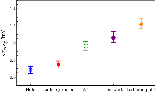
The mass and scalar radii provide complementary information on the spatial structure of the gluonic contribution to the proton. The mass radius characterizes the spatial distribution of the gluon energy contribution, while the scalar radius is associated with the scalar part of the gluon EMT and provides information on the related mechanical structure. The difference between these two radii originates from the different combinations of gluon GFFs entering their definitions. In particular, the scalar radius has a more direct dependence on the $D$ -term contribution, making it more sensitive to the details of its determination.

The comparison shown in Fig. 4 indicates that the gluon mass radius obtained in this work is consistent with the available results in the literature. In particular, the obtained value agrees well with the lattice QCD tripole-fit result and the $\xi>4$ approach, while the lattice QCD dipole-fit result yields a larger radius. The gluon scalar radius exhibits a wider spread among the available results. The value obtained in this work lies between the holographic prediction and the lattice QCD dipole-fit result, while remaining compatible with the lattice QCD tripole-fit and $\xi>4$ results within the quoted uncertainties.

These results indicate that the spatial distribution of the gluon energy inside the proton is relatively stable across different approaches, whereas the scalar structure shows a stronger dependence on the details of the employed determinations, consistent with its sensitivity to the $D$ -term contribution.

V SUMMARY AND CONCLUSION

The GFFs associated with the individual contributions to the proton EMT provide fundamental information about the internal structure of the proton, and their determination remains one of the central challenges in hadron physics. In this work, we have investigated the gluon and photon contributions to the gravitational structure of the proton within the QCDSR framework. This study provides an independent QCDSR investigation of these sectors and complements previous studies of the proton gravitational structure.

The correlation function was constructed from both the physical and QCD representations. On the physical side, the matrix element of the EMT was decomposed into independent Lorentz structures parameterized by the GFFs. On the QCD side, the gluon contribution was evaluated by taking into account both the vacuum expectation value of the gluon field-strength tensors and the quark–gluon interaction effects included through the corresponding correction to the quark propagator. The photon contribution was incorporated through the quark–photon interaction effects entering via the corresponding quark propagator correction.

Since the present study focuses only on the gluon and photon contributions to the proton EMT, without including the quark sector, these two sectors are described by four independent GFFs. This allows the corresponding non-conserved form factor contribution, represented by $\bar{c}^{j}(Q^{2})$ , to be consistently taken into account in the determination of the proton gravitational structure.

The obtained gluon GFFs provide insight into the energy and angular momentum distributions carried by the gluons inside the proton. The values of the gluon energy and angular momentum form factors at zero momentum transfer are found to be consistent with previous theoretical results, supporting the extraction of the gluon contribution to the proton momentum and spin structure. In contrast, the $D$ -term shows a stronger sensitivity to different theoretical approaches, reflecting its dependence on the details of the nonperturbative dynamics and the extraction methodology.

Furthermore, the non-conserved form factor $\bar{c}^{g}(Q^{2})$ has been explicitly retained in the present analysis due to the separate treatment of the gluon sector. This leads to a more complete description of the gluon contribution to the proton EMT without imposing the constraints that arise when the quark and gluon contributions are combined.

The photon contribution to the proton EMT is found to be much smaller than the gluon contribution, reflecting the subleading role of the electromagnetic sector in the proton gravitational structure. Nevertheless, its explicit determination provides complementary information on the electromagnetic contribution to the proton EMT.

Beyond the $Q^{2}$ -dependence of the GFFs, we further investigated the spatial structure of the gluon and photon contributions through the corresponding mass and scalar radii of the proton. The obtained gluon mass radius is found to be consistent with previous theoretical predictions, indicating a relatively stable spatial distribution of the gluon energy inside the proton. In contrast, the gluon scalar radius exhibits a larger variation among different approaches due to its stronger sensitivity to the $D$ -term contribution. The calculated photon radii provide an estimate of the spatial extent of the electromagnetic contribution to the proton EMT.

The results obtained in this work show that the QCDSR framework provides a consistent approach for investigating the separate gluon and photon contributions to the gravitational structure of the proton. These results can serve as a basis for further investigations of the proton gravitational structure and more comprehensive studies of the QCD energy-momentum tensor.

ACKNOWLEDGMENTS

K. Azizi thanks Iran national science foundation (INSF) for the partial financial support supplied under the elites Grant No. 40405095.

Declaration of AI-assisted language editing

The authors have used AI tools, only for language editing and improving the readability of the manuscript. The authors have reviewed and edited the manuscript and take full responsibility for its scientific content.

Appendix A The functions of physical side

In this appendix, we present the invariant amplitudes $\Pi_{i}^{\mathrm{phy},\,j}(Q^{2})$ obtained from the physical representation of the correlation function. Their dependence on the GFFs and the relevant physical parameters of the proton is explicitly shown as follows:

\displaystyle\begin{array}[]{l@{\hspace{2cm}}l@{\hspace{2cm}}l}\Pi_{1}^{\mathrm{phy},\,j}(Q^{2})=\dfrac{m}{4}\,\Big(A^{j}(Q^{2})+D^{j}(Q^{2})\Big),\hfil\hskip 56.9055pt&\Pi_{6}^{\mathrm{phy},\,j}(Q^{2})=\dfrac{1}{4m}\,\Big(A^{j}(Q^{2})+D^{j}(Q^{2})-J^{j}(Q^{2})\Big),\hfil\hskip 56.9055pt\\ \hfil\hskip 56.9055pt\\ \Pi_{2}^{\mathrm{phy},\,j}(Q^{2})=\dfrac{m}{4}\,\Big(A^{j}(Q^{2})-D^{j}(Q^{2})\Big),\hfil\hskip 56.9055pt&\Pi_{7}^{\mathrm{phy},\,j}(Q^{2})=\dfrac{1}{4m}\,\Big(A^{j}(Q^{2})-D^{j}(Q^{2})-J^{j}(Q^{2})\Big),\hfil\hskip 56.9055pt\\ \hfil\hskip 56.9055pt\\ \Pi_{3}^{\mathrm{phy},\,j}(Q^{2})=\dfrac{1}{4}\,\Big(A^{j}(Q^{2})+D^{j}(Q^{2})\Big),\hfil\hskip 56.9055pt&\Pi_{8}^{\mathrm{phy},\,j}(Q^{2})=\dfrac{1}{4m}\,\Big(A^{j}(Q^{2})-D^{j}(Q^{2})-2J^{j}(Q^{2})\Big),\hfil\hskip 56.9055pt\\ \hfil\hskip 56.9055pt\\ \Pi_{4}^{\mathrm{phy},\,j}(Q^{2})=\dfrac{1}{4}\,\Big(A^{j}(Q^{2})-D^{j}(Q^{2})\Big),\hfil\hskip 56.9055pt&\Pi_{9}^{\mathrm{phy},\,j}(Q^{2})=\dfrac{1}{4m}\,\Big(A^{j}(Q^{2})+D^{j}(Q^{2})-2J^{j}(Q^{2})\Big),\hfil\hskip 56.9055pt\\ \hfil\hskip 56.9055pt\\ \Pi_{5}^{\mathrm{phy},\,j}(Q^{2})=m^{2}\bar{c}^{j}(Q^{2})-\dfrac{1}{4}D^{j}(Q^{2})\hfil\hskip 56.9055pt&\Pi_{10}^{\mathrm{phy},\,j}(Q^{2})=m\bar{c}^{j}(Q^{2})-\dfrac{1}{4m}D^{j}(Q^{2}).\hfil\hskip 56.9055pt\end{array}

Appendix B QCD side Results

In this appendix, we provide the explicit form for the QCD side contributions arising from the gluon and photon EMT insertions.

B. 1 First class of gluonic contributions

The explicit expression for $\Pi_{\mu\nu}^{g,\,(1)}(x,y)$ is given as

$\displaystyle\Pi_{\mu\nu}^{g,\,(1)}(x,y)=2\,\langle G^{2}\rangle\,g_{\mu\nu}\,\Bigg($	$\displaystyle-\Big[\gamma_{5}\,S_{u}^{ca^{\prime}}(y-x)\,S_{d}^{{}^{\prime}\,bb^{\prime}}(y-x)\,S_{u}^{ac^{\prime}}(y-x)\,\gamma_{5}\Big]+\Big[\gamma_{5}\,S_{u}^{cc^{\prime}}(y-x)\,\gamma_{5}\Big]\,\text{Tr}\Big[S_{u}^{{}^{\prime}\,aa^{\prime}}(y-x)\,S_{d}^{bb^{\prime}}(y-x)\Big]$
	$\displaystyle-\beta\Big[\gamma_{5}\,S_{u}^{cc^{\prime}}(y-x)\Big]\,\text{Tr}\Big[\gamma_{5}\,S_{u}^{{}^{\prime}\,aa^{\prime}}(y-x)\,S_{d}^{bb^{\prime}}(y-x)\Big]+\beta\Big[\gamma_{5}\,S_{u}^{ca^{\prime}}(y-x)\,\gamma_{5}\,S_{d}^{\prime bb^{\prime}}(y-x)\,S_{u}^{ac^{\prime}}(y-x)\Big]$
	$\displaystyle-\beta\,\Big[S_{u}^{ca^{\prime}}(y-x)\,S^{\prime bb^{\prime}}_{d}(y-x)\,\gamma_{5}\,S_{u}^{ac^{\prime}}(y-x)\,\gamma_{5}\Big]+\beta\,\Big[S^{cc^{\prime}}_{u}(y-x)\,\gamma_{5}\Big]\,\text{Tr}\Big[S^{\prime aa^{\prime}}_{u}(y-x)\,\gamma_{5}\,S^{bb^{\prime}}_{d}(y-x)\Big]$
	$\displaystyle+\beta^{2}\,\Big[S_{u}^{ca^{\prime}}(y-x)\,\gamma_{5}\,S^{\prime bb^{\prime}}_{d}(y-x)\,\gamma_{5}\,S_{u}^{ac^{\prime}}(y-x)\Big]-\beta^{2}\,\Big[S_{u}^{cc^{\prime}}(y-x)\Big]\,\text{Tr}\Big[S^{\prime aa^{\prime}}_{u}(y-x)\,\gamma_{5}\,S_{d}^{bb^{\prime}}(y-x)\,\gamma_{5}\Big]\Bigg).$	(59)

where $S_{\psi}^{ab}(x)$ , with $\psi=u,d$ , denotes the light-quark propagator in coordinate space, while $S_{\psi}^{\prime\,ab}(x)=C\left[S_{\psi}^{ab}(x)\right]^{T}C$ represents the corresponding charge-conjugated propagator. The light-quark propagator, including perturbative and nonperturbative contributions, is expressed in coordinate space as [79],

	$\displaystyle S_{\psi}^{ab}(x)$	$\displaystyle=i\delta^{ab}\frac{\not{x}}{2\pi^{2}x^{4}}-\delta^{ab}\frac{m_{\psi}}{4\pi^{2}x^{2}}-\delta^{ab}\frac{\langle\bar{\psi}\psi\rangle}{12}\bigg(1-\frac{m_{\psi}\not{x}}{4}\bigg)-\delta^{ab}\frac{x^{2}}{192}\left\langle\bar{\psi}g_{s}\sigma G\psi\right\rangle\bigg(1-i\frac{m_{\psi}\not{x}}{6}\bigg)$
		$\displaystyle-i\frac{g_{s}G^{ab}_{\alpha\beta}}{32\pi^{2}x^{2}}\left[\not{x}\sigma^{\alpha\beta}+\sigma^{\alpha\beta}\not{x}\right]-i\delta^{ab}\frac{x^{2}\not{x}g_{s}^{2}\langle\bar{\psi}\psi\rangle^{2}}{7776}+\cdots,$		(60)

where $m_{\psi}$ denotes the light-quark mass. The quantities $\langle\bar{\psi}\psi\rangle$ , $\langle G^{2}\rangle$ , and $\langle\bar{\psi}g_{s}\sigma G\psi\rangle$ correspond to the quark, gluon, and mixed quark-gluon condensates, respectively. The gluon field strength tensor appearing in the quark propagator is defined as [59, 60],

\displaystyle G_{\alpha\beta}^{ab}=G_{\alpha\beta}^{A}T_{A}^{ab},\qquad T_{A}=\frac{1}{2}\lambda_{A},\qquad G^{2}=G_{\alpha\beta}^{A}G_{\alpha\beta}^{A},

(61)

where $a,b=1,2,3$ and $A=1,\dots,8$ denote the color indices of the quark and gluon fields, respectively. Here, $\lambda_{A}$ are the Gell-Mann matrices and $T_{A}$ are the generators of the $SU(3)$ color group in the fundamental representation. The vacuum expectation value of two gluon field strength tensors in the adjoint color representation is given by [59, 60],

\displaystyle\langle G_{\alpha^{\prime}\beta^{\prime}}^{A_{1}}G_{\alpha\beta}^{A_{2}}\rangle=\frac{\delta^{A_{1}A_{2}}}{96}\,\langle G^{2}\rangle\left(g_{\alpha^{\prime}\alpha}g_{\beta^{\prime}\beta}-g_{\alpha^{\prime}\beta}g_{\beta^{\prime}\alpha}\right).

(62)

In obtaining Eq. (59), the vacuum expectation value of the gluon field strength tensors is evaluated using Eq. (62).

B. 2 Second class of gluonic contributions

The resulting expression $\Pi_{\mu\nu}^{g,\,(2)}(x,y)$ for the second class contribution, obtained from the gluon-induced correction to the light-quark propagators, is given as

$\displaystyle\Pi_{\mu\nu}^{g,\,(2)}(x,y)=4$	$\displaystyle\,\Bigg(-\Big[\gamma_{5}\,\Delta S_{u}^{ca^{\prime},\,g}(y-x)\,S_{d}^{{}^{\prime}\,bb^{\prime}}(y-x)\,S_{u}^{ac^{\prime}}(y-x)\,\gamma_{5}\Big]-\Big[\gamma_{5}\,S_{u}^{ca^{\prime}}(y-x)\,\Delta S_{d}^{{}^{\prime}\,bb^{\prime},\,g}(y-x)\,S_{u}^{ac^{\prime}}(y-x)\,\gamma_{5}\Big]$
	$\displaystyle~~~-\Big[\gamma_{5}\,S_{u}^{ca^{\prime}}(y-x)\,S_{d}^{{}^{\prime}\,bb^{\prime}}(y-x)\,\Delta S_{u}^{ac^{\prime},\,g}(y-x)\,\gamma_{5}\Big]+\Big[\gamma_{5}\,\Delta S_{u}^{cc^{\prime},\,g}(y-x)\,\gamma_{5}\Big]\,\text{Tr}\Big[S_{u}^{{}^{\prime}\,aa^{\prime}}(y-x)\,S_{d}^{bb^{\prime}}(y-x)\Big]$
	$\displaystyle~~~+\Big[\gamma_{5}\,S_{u}^{cc^{\prime}}(y-x)\,\gamma_{5}\Big]\,\text{Tr}\Big[\Delta S_{u}^{{}^{\prime}\,aa^{\prime},\,g}(y-x)\,S_{d}^{bb^{\prime}}(y-x)\Big]+\Big[\gamma_{5}\,S_{u}^{cc^{\prime}}(y-x)\,\gamma_{5}\Big]\,\text{Tr}\Big[S_{u}^{{}^{\prime}\,aa^{\prime}}(y-x)\,\Delta S_{d}^{bb^{\prime},\,g}(y-x)\Big]$
	$\displaystyle~~~-\beta\Big[\gamma_{5}\,\Delta S_{u}^{cc^{\prime},\,g}(y-x)\Big]\,\text{Tr}\Big[\gamma_{5}\,S_{u}^{{}^{\prime}\,aa^{\prime}}(y-x)\,S_{d}^{bb^{\prime}}(y-x)\Big]-\beta\Big[\gamma_{5}\,S_{u}^{cc^{\prime}}(y-x)\Big]\,\text{Tr}\Big[\gamma_{5}\,\Delta S_{u}^{{}^{\prime}\,aa^{\prime},\,g}(y-x)\,S_{d}^{bb^{\prime}}(y-x)\Big]$
	$\displaystyle~~~-\beta\Big[\gamma_{5}\,S_{u}^{cc^{\prime}}(y-x)\Big]\,\text{Tr}\Big[\gamma_{5}\,S_{u}^{{}^{\prime}\,aa^{\prime}}(y-x)\,\Delta S_{d}^{bb^{\prime},\,g}(y-x)\Big]+\beta\Big[\gamma_{5}\,\Delta S_{u}^{ca^{\prime},\,g}(y-x)\,\gamma_{5}\,S_{d}^{\prime bb^{\prime}}(y-x)\,S_{u}^{ac^{\prime}}(y-x)\Big]$
	$\displaystyle~~~+\beta\Big[\gamma_{5}\,S_{u}^{ca^{\prime}}(y-x)\,\gamma_{5}\,\Delta S_{d}^{\prime bb^{\prime},\,g}(y-x)\,S_{u}^{ac^{\prime}}(y-x)\Big]+\beta\Big[\gamma_{5}\,S_{u}^{ca^{\prime}}(y-x)\,\gamma_{5}\,S_{d}^{\prime bb^{\prime}}(y-x)\,\Delta S_{u}^{ac^{\prime},\,g}(y-x)\Big]$
	$\displaystyle~~~-\beta\,\Big[\Delta S_{u}^{ca^{\prime},\,g}(y-x)\,S^{\prime bb^{\prime}}_{d}(y-x)\,\gamma_{5}\,S_{u}^{ac^{\prime}}(y-x)\,\gamma_{5}\Big]-\beta\,\Big[S_{u}^{ca^{\prime}}(y-x)\,\Delta S^{\prime bb^{\prime},\,g}_{d}(y-x)\,\gamma_{5}\,S_{u}^{ac^{\prime}}(y-x)\,\gamma_{5}\Big]$
	$\displaystyle~~~-\beta\,\Big[S_{u}^{ca^{\prime}}(y-x)\,S^{\prime bb^{\prime}}_{d}(y-x)\,\gamma_{5}\,\Delta S_{u}^{ac^{\prime},\,g}(y-x)\,\gamma_{5}\Big]+\beta\,\Big[\Delta S^{cc^{\prime},\,g}_{u}(y-x)\,\gamma_{5}\Big]\,\text{Tr}\Big[S^{\prime aa^{\prime}}_{u}(y-x)\,\gamma_{5}\,S^{bb^{\prime}}_{d}(y-x)\Big]$
	$\displaystyle~~~+\beta\,\Big[S^{cc^{\prime}}_{u}(y-x)\,\gamma_{5}\Big]\,\text{Tr}\Big[\Delta S^{\prime aa^{\prime},\,g}_{u}(y-x)\,\gamma_{5}\,S^{bb^{\prime}}_{d}(y-x)\Big]+\beta\,\Big[S^{cc^{\prime}}_{u}(y-x)\,\gamma_{5}\Big]\,\text{Tr}\Big[S^{\prime aa^{\prime}}_{u}(y-x)\,\gamma_{5}\,\Delta S^{bb^{\prime},\,g}_{d}(y-x)\Big]$
	$\displaystyle~~~+\beta^{2}\,\Big[\Delta S_{u}^{ca^{\prime},\,g}(y-x)\,\gamma_{5}\,S^{\prime bb^{\prime}}_{d}(y-x)\,\gamma_{5}\,S_{u}^{ac^{\prime}}(y-x)\Big]+\beta^{2}\,\Big[S_{u}^{ca^{\prime}}(y-x)\,\gamma_{5}\,\Delta S^{\prime bb^{\prime},\,g}_{d}(y-x)\,\gamma_{5}\,S_{u}^{ac^{\prime}}(y-x)\Big]$
	$\displaystyle~~~+\beta^{2}\,\Big[S_{u}^{ca^{\prime}}(y-x)\,\gamma_{5}\,S^{\prime bb^{\prime}}_{d}(y-x)\,\gamma_{5}\,\Delta S_{u}^{ac^{\prime},\,g}(y-x)\Big]-\beta^{2}\,\Big[\Delta S_{u}^{cc^{\prime},\,g}(y-x)\Big]\,\text{Tr}\Big[S^{\prime aa^{\prime}}_{u}(y-x)\,\gamma_{5}\,S_{d}^{bb^{\prime}}(y-x)\,\gamma_{5}\Big]$
	$\displaystyle~~~-\beta^{2}\,\Big[S_{u}^{cc^{\prime}}(y-x)\Big]\,\text{Tr}\Big[\Delta S^{\prime aa^{\prime},\,g}_{u}(y-x)\,\gamma_{5}\,S_{d}^{bb^{\prime}}(y-x)\,\gamma_{5}\Big]-\beta^{2}\,\Big[S_{u}^{cc^{\prime}}(y-x)\Big]\,\text{Tr}\Big[S^{\prime aa^{\prime}}_{u}(y-x)\,\gamma_{5}\,\Delta S_{d}^{bb^{\prime},\,g}(y-x)\,\gamma_{5}\Big]\Bigg).$	(63)

B. 3 Photonic contributions

After performing the Fourier transformation of the coordinate-space light-quark propagators and employing the momentum-space representation of the free photon propagator, the photon-induced correction to the light-quark propagator can be written as

$\displaystyle\Delta S_{u}^{ca^{\prime},\,\gamma}$	$\displaystyle=-\frac{e_{u}^{2}}{2}\int d^{4}z_{1}\int d^{4}z_{2}\left[-\int\frac{d^{4}k_{1}}{(2\pi)^{4}}\frac{d^{4}k_{2}}{(2\pi)^{4}}\frac{N_{\alpha\beta\mu\nu}(k_{1},k_{2})}{(k_{1}^{2}+i\epsilon)(k_{2}^{2}+i\epsilon)}e^{-ik_{1}\cdot z_{1}}e^{-ik_{2}\cdot z_{2}}\right]$
	$\displaystyle\qquad\times\Bigg[\int\frac{d^{4}p_{1}}{(2\pi)^{4}}e^{-ip_{1}\cdot(y-z_{1})}S_{u}^{ci}(p_{1})\gamma^{\alpha}\int\frac{d^{4}p_{2}}{(2\pi)^{4}}e^{-ip_{2}\cdot(z_{1}-z_{2})}S_{u}^{ij}(p_{2})\gamma^{\beta}\int\frac{d^{4}p_{3}}{(2\pi)^{4}}e^{-ip_{3}\cdot(z_{2}-x)}S_{u}^{ja^{\prime}}(p_{3})$
	$\displaystyle\qquad~~~~~+\int\frac{d^{4}p_{1}}{(2\pi)^{4}}e^{-ip_{1}\cdot(y-z_{2})}S_{u}^{ci}(p_{1})\gamma^{\beta}\int\frac{d^{4}p_{2}}{(2\pi)^{4}}e^{-ip_{2}\cdot(z_{2}-z_{1})}S_{u}^{ij}(p_{2})\gamma^{\alpha}\int\frac{d^{4}p_{3}}{(2\pi)^{4}}e^{-ip_{3}\cdot(z_{1}-x)}S_{u}^{ja^{\prime}}(p_{3})\Bigg],$	(64)

where the momentum-dependent tensor $N_{\alpha\beta\mu\nu}(k_{1},k_{2})$ is defined as

	$\displaystyle N_{\alpha\beta\mu\nu}(k_{1},k_{2})$	$\displaystyle=\Big[(k_{1\mu}g_{\alpha\rho}-k_{1\rho}g_{\alpha\mu})(k_{2\nu}g_{\beta}^{\ \rho}-k_{2}^{\rho}g_{\beta\nu})+(k_{1\nu}g_{\alpha\rho}-k_{1\rho}g_{\alpha\nu})(k_{2\mu}g_{\beta}^{\ \rho}-k_{2}^{\rho}g_{\beta\mu})\Big]$
		$\displaystyle~~~-\frac{1}{4}g_{\mu\nu}\Big[(k_{1\rho}g_{\alpha\sigma}-k_{1\sigma}g_{\alpha\rho})(k_{2}^{\rho}g_{\beta}^{\ \sigma}-k_{2}^{\sigma}g_{\beta}^{\ \rho})+(k_{2\rho}g_{\alpha\sigma}-k_{2\sigma}g_{\alpha\rho})(k_{1}^{\rho}g_{\beta}^{\ \sigma}-k_{1}^{\sigma}g_{\beta}^{\ \rho})\Big].$		(65)

The explicit expression for $\Pi_{\mu\nu}^{\gamma}$ appearing in Eq. (42) is given by

$\displaystyle\Pi_{\mu\nu}^{\gamma}=4$	$\displaystyle\,\Bigg(-\Big[\gamma_{5}\,\Delta S_{u}^{ca^{\prime},\,\gamma}\,S_{d}^{{}^{\prime}\,bb^{\prime}}\,S_{u}^{ac^{\prime}}\,\gamma_{5}\Big]-\Big[\gamma_{5}\,S_{u}^{ca^{\prime}}\,\Delta S_{d}^{{}^{\prime}\,bb^{\prime},\,\gamma}\,S_{u}^{ac^{\prime}}\,\gamma_{5}\Big]-\Big[\gamma_{5}\,S_{u}^{ca^{\prime}}\,S_{d}^{{}^{\prime}\,bb^{\prime}}\,\Delta S_{u}^{ac^{\prime},\,\gamma}\,\gamma_{5}\Big]$
	$\displaystyle~~~+\Big[\gamma_{5}\,\Delta S_{u}^{cc^{\prime},\,\gamma}\,\gamma_{5}\Big]\,\text{Tr}\Big[S_{u}^{{}^{\prime}\,aa^{\prime}}\,S_{d}^{bb^{\prime}}\Big]+\Big[\gamma_{5}\,S_{u}^{cc^{\prime}}\,\gamma_{5}\Big]\,\text{Tr}\Big[\Delta S_{u}^{{}^{\prime}\,aa^{\prime},\,\gamma}\,S_{d}^{bb^{\prime}}\Big]+\Big[\gamma_{5}\,S_{u}^{cc^{\prime}}\,\gamma_{5}\Big]\,\text{Tr}\Big[S_{u}^{{}^{\prime}\,aa^{\prime}}\,\Delta S_{d}^{bb^{\prime},\,\gamma}\Big]$
	$\displaystyle~~~-\beta\Big[\gamma_{5}\,\Delta S_{u}^{cc^{\prime},\,\gamma}\Big]\,\text{Tr}\Big[\gamma_{5}\,S_{u}^{{}^{\prime}\,aa^{\prime}}\,S_{d}^{bb^{\prime}}\Big]-\beta\Big[\gamma_{5}\,S_{u}^{cc^{\prime}}\Big]\,\text{Tr}\Big[\gamma_{5}\,\Delta S_{u}^{{}^{\prime}\,aa^{\prime},\,\gamma}\,S_{d}^{bb^{\prime}}\Big]-\beta\Big[\gamma_{5}\,S_{u}^{cc^{\prime}}\Big]\,\text{Tr}\Big[\gamma_{5}\,S_{u}^{{}^{\prime}\,aa^{\prime}}\,\Delta S_{d}^{bb^{\prime},\,\gamma}\Big]$
	$\displaystyle~~~+\beta\Big[\gamma_{5}\,\Delta S_{u}^{ca^{\prime},\,\gamma}\,\gamma_{5}\,S_{d}^{\prime bb^{\prime}}\,S_{u}^{ac^{\prime}}\Big]+\beta\Big[\gamma_{5}\,S_{u}^{ca^{\prime}}\,\gamma_{5}\,\Delta S_{d}^{\prime bb^{\prime},\,\gamma}\,S_{u}^{ac^{\prime}}\Big]+\beta\Big[\gamma_{5}\,S_{u}^{ca^{\prime}}\,\gamma_{5}\,S_{d}^{\prime bb^{\prime}}\,\Delta S_{u}^{ac^{\prime},\,\gamma}\Big]$
	$\displaystyle~~~-\beta\,\Big[\Delta S_{u}^{ca^{\prime},\,\gamma}\,S^{\prime bb^{\prime}}_{d}\,\gamma_{5}\,S_{u}^{ac^{\prime}}\,\gamma_{5}\Big]-\beta\,\Big[S_{u}^{ca^{\prime}}\,\Delta S^{\prime bb^{\prime},\,\gamma}_{d}\,\gamma_{5}\,S_{u}^{ac^{\prime}}\,\gamma_{5}\Big]-\beta\,\Big[S_{u}^{ca^{\prime}}\,S^{\prime bb^{\prime}}_{d}\,\gamma_{5}\,\Delta S_{u}^{ac^{\prime},\,\gamma}\,\gamma_{5}\Big]$
	$\displaystyle~~~+\beta\,\Big[\Delta S^{cc^{\prime},\,\gamma}_{u}\,\gamma_{5}\Big]\,\text{Tr}\Big[S^{\prime aa^{\prime}}_{u}\,\gamma_{5}\,S^{bb^{\prime}}_{d}\Big]+\beta\,\Big[S^{cc^{\prime}}_{u}\,\gamma_{5}\Big]\,\text{Tr}\Big[\Delta S^{\prime aa^{\prime},\,\gamma}_{u}\,\gamma_{5}\,S^{bb^{\prime}}_{d}\Big]+\beta\,\Big[S^{cc^{\prime}}_{u}\,\gamma_{5}\Big]\,\text{Tr}\Big[S^{\prime aa^{\prime}}_{u}\,\gamma_{5}\,\Delta S^{bb^{\prime},\,\gamma}_{d}\Big]$
	$\displaystyle~~~+\beta^{2}\,\Big[\Delta S_{u}^{ca^{\prime},\,\gamma}\,\gamma_{5}\,S^{\prime bb^{\prime}}_{d}\,\gamma_{5}\,S_{u}^{ac^{\prime}}\Big]+\beta^{2}\,\Big[S_{u}^{ca^{\prime}}\,\gamma_{5}\,\Delta S^{\prime bb^{\prime},\,\gamma}_{d}\,\gamma_{5}\,S_{u}^{ac^{\prime}}\Big]+\beta^{2}\,\Big[S_{u}^{ca^{\prime}}\,\gamma_{5}\,S^{\prime bb^{\prime}}_{d}\,\gamma_{5}\,\Delta S_{u}^{ac^{\prime},\,\gamma}\Big]$
	$\displaystyle~~~-\beta^{2}\,\Big[\Delta S_{u}^{cc^{\prime},\,\gamma}\Big]\,\text{Tr}\Big[S^{\prime aa^{\prime}}_{u}\,\gamma_{5}\,S_{d}^{bb^{\prime}}\,\gamma_{5}\Big]-\beta^{2}\,\Big[S_{u}^{cc^{\prime}}\Big]\,\text{Tr}\Big[\Delta S^{\prime aa^{\prime},\,\gamma}_{u}\,\gamma_{5}\,S_{d}^{bb^{\prime}}\,\gamma_{5}\Big]-\beta^{2}\,\Big[S_{u}^{cc^{\prime}}\Big]\,\text{Tr}\Big[S^{\prime aa^{\prime}}_{u}\,\gamma_{5}\,\Delta S_{d}^{bb^{\prime},\,\gamma}\,\gamma_{5}\Big]\Bigg).$	(66)

Appendix C Derivation of the Mass and Scalar Radii

In this appendix, we derive Eq. (48) for the mass and scalar radii used in this work. The commonly used relations for the mass and scalar radii in the literature [47, 80] are derived within the framework of the complete proton EMT, where both quark and gluon contributions are taken into account. In this framework, relations among the GFFs and the cancellation of the non-conserved contributions between different sectors lead to simplified expressions for the corresponding radii. However, the present analysis focuses on the gluon and photon sectors of the proton EMT, without including the quark contribution. Consequently, the non-conserved form factor $\bar{c}^{j}(t)$ contributes explicitly and must be retained throughout the derivation. The derivations of the mass and scalar radii are presented separately.

C. 1 Derivation of the Mass Radius

The mass radius associated with an individual EMT contribution $j$ is defined as the normalized second moment of the corresponding energy density,

\displaystyle\langle r_{m}^{2}\rangle_{j}=\frac{\displaystyle\int d^{3}r\,r^{2}\varepsilon_{j}(r)}{\displaystyle\int d^{3}r\,\varepsilon_{j}(r)}.

(67)

To express this quantity in terms of the GFFs, the corresponding energy density in the Breit frame is required. It is defined through the temporal component of the EMT as

\displaystyle\varepsilon_{j}(r)=T_{00}^{j}(r).

(68)

The three-dimensional Fourier transform of a GFF is defined as

\displaystyle[f(t)]_{\rm FT}=\int\frac{d^{3}\bm{\Delta}}{(2\pi)^{3}}e^{-i\bm{\Delta}\cdot\mathbf{r}}f(t),\qquad t=\Delta^{2}=-\bm{\Delta}^{\,2}.

(69)

Using the general decomposition of the EMT matrix element given in Eq. (5), the energy density defined in Eq. (68) can be expressed as

\displaystyle\varepsilon_{j}(r)=M_{N}\Big[A_{j}(t)+\bar{c}_{j}(t)-\frac{t}{4M_{N}^{2}}\left(A_{j}(t)-2J_{j}(t)+D_{j}(t)\right)\Big]_{\rm FT}.

(70)

The normalization of the energy density is obtained from the zeroth moment of the Fourier transform,

\displaystyle\int d^{3}r\,\varepsilon_{j}(r)=M_{N}\big[A_{j}(0)+\bar{c}_{j}(0)\big].

(71)

Expanding the GFFs around the forward limit, $t=0$ , we write

\displaystyle F_{j}(t)=F_{j}(0)+tF_{j}^{\prime}(0)+{\cal O}(t^{2}),

(72)

where $F_{j}=\{A_{j},\bar{c}_{j},J_{j},D_{j}\}$ . Using the standard property of the three-dimensional Fourier transform defined in Eq. (69),

\displaystyle\int d^{3}r\,r^{2}[f(t)]_{\rm FT}=6\left.\frac{df(t)}{dt}\right|_{t=0},

(73)

the second moment of the energy density can be evaluated. Substituting the resulting relation into Eq. (67), we obtain

\displaystyle\langle r_{m}^{2}\rangle_{j}=\frac{1}{A_{j}(0)+\bar{c}_{j}(0)}\left[6\left.\frac{dA_{j}(t)}{dt}\right|_{t=0}+6\left.\frac{d\bar{c}_{j}(t)}{dt}\right|_{t=0}-\frac{3}{2M_{N}^{2}}\left(A_{j}(0)-2J_{j}(0)+D_{j}(0)\right)\right].

(74)

Unlike the case of the complete proton EMT, Eq. (74) contains an explicit contribution from the non-conserved form factor $\bar{c}_{j}(t)$ . This term vanishes only after combining the contributions from all EMT sectors. Since the quark contribution to the proton EMT is not included in the present work, the $\bar{c}_{j}(t)$ contribution is retained throughout the derivation.

For comparison, we now show that Eq. (74) reduces to the commonly used relation when the complete proton EMT is considered. In this case, using the forward limit relations adopted in previous studies,

\displaystyle J_{q}(0)+J_{g}(0)=\frac{1}{2},\qquad A_{q}(0)+A_{g}(0)=1,\qquad\bar{c}_{q}(0)+\bar{c}_{g}(0)=0,

(75)

and substituting these relations into Eq. (74), one recovers the form used in previous studies [47, 80], after adopting the convention $D_{j}(t)=4C_{j}(t)$ for the parametrization of the $D$ -term contribution,

\displaystyle\langle r_{m}^{2}\rangle_{j}=\frac{1}{A_{j}(0)}\left[6\left.\frac{dA_{j}(t)}{dt}\right|_{t=0}-6\,\frac{C_{j}(0)}{M_{N}^{2}}\right].

(76)

C. 2 Derivation of the Scalar Radius

The scalar radius associated with an individual EMT contribution $j$ is defined as the normalized second moment of the corresponding scalar density,

\displaystyle\langle r_{s}^{2}\rangle_{j}=\frac{\displaystyle\int d^{3}r\,r^{2}\rho_{j}(r)}{\displaystyle\int d^{3}r\,\rho_{j}(r)}.

(77)

The scalar density is obtained from the spatial distribution of the trace of the EMT in the Breit frame. In contrast to the mass radius, which is related to the temporal component $T_{00}$ , the scalar radius is determined from the trace contribution

\displaystyle T^{\mu}_{\ \mu}=g^{\mu\nu}T_{\mu\nu}.

(78)

Using the general EMT decomposition given in Eq. (5), the trace of the EMT matrix element leads to the following scalar density:

\displaystyle\rho_{j}(r)=M_{N}\left[A_{j}(t)+\bar{c}_{j}(t)-\frac{3t}{4M_{N}^{2}}D_{j}(t)\right]_{\rm FT}.

(79)

Here, the angular momentum form factor $J_{j}(t)$ does not contribute to the trace due to the antisymmetric structure of the tensor $\sigma_{\mu\nu}$ . The non-conserved form factor $\bar{c}_{j}(t)$ is retained in the above relation because the EMT contribution $j$ is considered separately.

The normalization of the scalar density is obtained from the zero momentum transfer limit of the Fourier transform,

\displaystyle\int d^{3}r\,\rho_{j}(r)=M_{N}\left[A_{j}(0)+\bar{c}_{j}(0)\right].

(80)

Using the expansion of the GFFs around the forward limit and the Fourier transform property given in Eqs. (72) and (73), the second moment of the scalar density can be evaluated as

\displaystyle\int d^{3}r\,r^{2}\rho_{j}(r)=6M_{N}\left[\left.\frac{dA_{j}(t)}{dt}\right|_{t=0}+\left.\frac{d\bar{c}_{j}(t)}{dt}\right|_{t=0}-\frac{3}{4M_{N}^{2}}D_{j}(0)\right].

(81)

Substituting the numerator and denominator into Eq. (77), we obtain

\displaystyle\langle r_{s}^{2}\rangle_{j}=\frac{1}{A_{j}(0)+\bar{c}_{j}(0)}\left[6\left.\frac{dA_{j}(t)}{dt}\right|_{t=0}+6\left.\frac{d\bar{c}_{j}(t)}{dt}\right|_{t=0}-\frac{9}{2M_{N}^{2}}D_{j}(0)\right].

(82)

The above relation corresponds to the case considered in the present work, where the quark contribution to the proton EMT is not included and the non-conserved form factor $\bar{c}_{j}(t)$ is therefore retained.

For comparison, we also consider the case of the complete proton EMT, where both quark and gluon contributions are included. In this case, the forward limit relations among the GFFs can be applied. Using the relations given in Eq. (75) and substituting them into Eq. (82), one recovers the commonly used form of the scalar radius in previous studies [47, 80], after adopting the convention $D_{j}(t)=4C_{j}(t)$ for the parametrization of the $D$ -term contribution, which reads

\displaystyle\langle r_{s}^{2}\rangle_{j}=\frac{1}{A_{j}(0)}\left[6A^{\prime}_{j}(0)-\frac{18}{M_{N}^{2}}C_{j}(0)\right].

(83)

References

[1] R. Hofstadter, H. R. Fechter and J. A. McIntyre, High-Energy Electron Scattering and Nuclear Structure Determinations, Phys. Rev. 92, 978 (1953).
[2] R. Hofstadter, Electron scattering and nuclear structure, Rev. Mod. Phys. 28, 214-254 (1956).
[3] E. D. Bloom, D. H. Coward, H. C. DeStaebler, J. Drees, G. Miller, L. W. Mo, R. E. Taylor, M. Breidenbach, J. I. Friedman and G. C. Hartmann, et al. High-Energy Inelastic e p Scattering at 6-Degrees and 10-Degrees, Phys. Rev. Lett. 23, 930-934 (1969).
[4] M. Breidenbach, J. I. Friedman, H. W. Kendall, E. D. Bloom, D. H. Coward, H. C. DeStaebler, J. Drees, L. W. Mo and R. E. Taylor, Observed behavior of highly inelastic electron-proton scattering, Phys. Rev. Lett. 23, 935-939 (1969).
[5] M. Gell-Mann, A Schematic Model of Baryons and Mesons, Phys. Lett. 8, 214-215 (1964).
[6] H. Fritzsch, M. Gell-Mann and H. Leutwyler, Advantages of the Color Octet Gluon Picture, Phys. Lett. B 47, 365-368 (1973).
[7] D. J. Gross and F. Wilczek, Ultraviolet Behavior of Nonabelian Gauge Theories, Phys. Rev. Lett. 30, 1343-1346 (1973).
[8] H. D. Politzer, Reliable Perturbative Results for Strong Interactions?, Phys. Rev. Lett. 30, 1346-1349 (1973).
[9] G. Zweig, An SU(3) model for strong interaction symmetry and its breaking. Version 2, CERN-TH-412.
[10] X. D. Ji, Deeply virtual Compton scattering, Phys. Rev. D 55, 7114-7125 (1997), [arXiv:hep-ph/9609381 [hep-ph]].
[11] D. Müller, D. Robaschik, B. Geyer, F. M. Dittes and J. Hořejši, Wave functions, evolution equations and evolution kernels from light ray operators of QCD, Fortsch. Phys. 42, 101-141 (1994), [arXiv:hep-ph/9812448 [hep-ph]].
[12] A. V. Radyushkin, Scaling limit of deeply virtual Compton scattering, Phys. Lett. B 380, 417-425 (1996), [arXiv:hep-ph/9604317 [hep-ph]].
[13] X. D. Ji, gauge-invariant Decomposition of Nucleon Spin, Phys. Rev. Lett. 78, 610-613 (1997), [arXiv:hep-ph/9603249 [hep-ph]].
[14] N. d’Hose, S. Niccolai and A. Rostomyan, Experimental overview of Deeply Virtual Compton Scattering, Eur. Phys. J. A 52, 151 (2016).
[15] K. Kumericki, S. Liuti and H. Moutarde, GPD phenomenology and DVCS fitting: Entering the high-precision era, Eur. Phys. J. A 52, 157 (2016), [arXiv:1602.02763 [hep-ph]].
[16] J. C. Collins, L. Frankfurt and M. Strikman, Factorization for hard exclusive electroproduction of mesons in QCD, Phys. Rev. D 56, 2982-3006 (1997), [arXiv:hep-ph/9611433 [hep-ph]].
[17] L. Mankiewicz, G. Piller, E. Stein, M. Vanttinen and T. Weigl, NLO corrections to deeply virtual Compton scattering, Phys. Lett. B 425, 186-192 (1998), [arXiv:hep-ph/9712251 [hep-ph]].
[18] V. D. Burkert, L. Elouadrhiri and F. X. Girod, The pressure distribution inside the proton, Nature 557, 396-399 (2018).
[19] V. D. Burkert, L. Elouadrhiri and F. X. Girod, Determination of shear forces inside the proton, [arXiv:2104.02031 [nucl-ex]].
[20] M. Gockeler et al. [QCDSF], Generalized parton distributions from lattice QCD, Phys. Rev. Lett. 92, 042002 (2004), [arXiv:hep-ph/0304249 [hep-ph]].
[21] P. Hagler et al. [LHPC and SESAM], Moments of nucleon generalized parton distributions in lattice QCD, Phys. Rev. D 68, 034505 (2003), [arXiv:hep-lat/0304018 [hep-lat]].
[22] P. E. Shanahan and W. Detmold, Pressure Distribution and Shear Forces inside the Proton, Phys. Rev. Lett. 122, 072003 (2019), [arXiv:1810.07589 [nucl-th]].
[23] M. Dorati, T. A. Gail and T. R. Hemmert, Chiral perturbation theory and the first moments of the generalized parton distributions in a nucleon, Nucl. Phys. A 798, 96-131 (2008), [arXiv:nucl-th/0703073 [nucl-th]].
[24] J. W. Chen and X. d. Ji, Leading chiral contributions to the spin structure of the proton, Phys. Rev. Lett. 88, 052003 (2002), [arXiv:hep-ph/0111048 [hep-ph]].
[25] K. Azizi and U. Özdem, Nucleon’s energy–momentum tensor form factors in light-cone QCD, Eur. Phys. J. C 80, 104 (2020), [arXiv:1908.06143 [hep-ph]].
[26] Z. Dehghan, F. Almaksusi and K. Azizi, Mechanical properties of proton using flavor-decomposed gravitational form factors, JHEP 06, 025 (2025), [arXiv:2502.16689 [hep-ph]].
[27] K. A. Mamo and I. Zahed, J/ $\psi$ near threshold in holographic QCD: A and D gravitational form factors, Phys. Rev. D 106, 086004 (2022), [arXiv:2204.08857 [hep-ph]].
[28] M. Fujita, Y. Hatta, S. Sugimoto and T. Ueda, Nucleon D-term in holographic quantum chromodynamics, PTEP 2022, 093B06 (2022), [arXiv:2206.06578 [hep-th]].
[29] C. Cebulla, K. Goeke, J. Ossmann and P. Schweitzer, The Nucleon form-factors of the energy momentum tensor in the Skyrme model, Nucl. Phys. A 794, 87-114 (2007), [arXiv:hep-ph/0703025 [hep-ph]].
[30] H. C. Kim, P. Schweitzer and U. Yakhshiev, Energy-momentum tensor form factors of the nucleon in nuclear matter, Phys. Lett. B 718, 625-631 (2012), [arXiv:1205.5228 [hep-ph]].
[31] C. Alexandrou, M. Constantinou, K. Hadjiyiannakou, K. Jansen, C. Kallidonis, G. Koutsou and A. Vaquero Avilés-Casco, Nucleon spin structure from lattice QCD, PoS DIS2018, 148 (2018), [arXiv:1807.11214 [hep-lat]].
[32] C. Alexandrou, S. Bacchio, M. Constantinou, J. Finkenrath, K. Hadjiyiannakou, K. Jansen, G. Koutsou, H. Panagopoulos and G. Spanoudes, Complete flavor decomposition of the spin and momentum fraction of the proton using lattice QCD simulations at physical pion mass, Phys. Rev. D 101, 094513 (2020), [arXiv:2003.08486 [hep-lat]].
[33] P. E. Shanahan and W. Detmold, Gluon gravitational form factors of the nucleon and the pion from lattice QCD, Phys. Rev. D 99, 014511 (2019), [arXiv:1810.04626 [hep-lat]].
[34] Y. B. Yang, M. Gong, J. Liang, H. W. Lin, K. F. Liu, D. Pefkou and P. Shanahan, Nonperturbatively renormalized glue momentum fraction at the physical pion mass from lattice QCD, Phys. Rev. D 98, 074506 (2018), [arXiv:1805.00531 [hep-lat]].
[35] Y. B. Yang, J. Liang, Y. J. Bi, Y. Chen, T. Draper, K. F. Liu and Z. Liu, Proton Mass Decomposition from the QCD Energy Momentum Tensor, Phys. Rev. Lett. 121, 212001 (2018), [arXiv:1808.08677 [hep-lat]].
[36] C. Alexandrou, M. Constantinou, K. Hadjiyiannakou, K. Jansen, C. Kallidonis, G. Koutsou, A. Vaquero Avilés-Casco and C. Wiese, Nucleon Spin and Momentum Decomposition Using Lattice QCD Simulations, Phys. Rev. Lett. 119, 142002 (2017), [arXiv:1706.02973 [hep-lat]].
[37] D. A. Pefkou, D. C. Hackett and P. E. Shanahan, Gluon gravitational structure of hadrons of different spin, Phys. Rev. D 105, 054509 (2022), [arXiv:2107.10368 [hep-lat]].
[38] D. C. Hackett, D. A. Pefkou and P. E. Shanahan, Gravitational Form Factors of the Proton from Lattice QCD, Phys. Rev. Lett. 132, 251904 (2024), [arXiv:2310.08484 [hep-lat]].
[39] B. Duran, Z. E. Meziani, S. Joosten, M. K. Jones, S. Prasad, C. Peng, W. Armstrong, H. Atac, E. Chudakov and H. Bhatt, et al. Determining the gluonic gravitational form factors of the proton, Nature 615, 813-816 (2023), [arXiv:2207.05212 [nucl-ex]].
[40] X. B. Tong, J. P. Ma and F. Yuan, Gluon gravitational form factors at large momentum transfer, Phys. Lett. B 823, 136751 (2021), [arXiv:2101.02395 [hep-ph]].
[41] P. C. Tandy, Gluon Parts of Gravitational Form Factors and Mass Distribution, PoS QCHSC24, 077 (2025), [arXiv:2505.00583 [nucl-th]].
[42] K. A. Mamo and I. Zahed, Diffractive photoproduction of $J/\psi$ and $\Upsilon$ using holographic QCD: gravitational form factors and GPD of gluons in the proton, Phys. Rev. D 101, 086003 (2020), [arXiv:1910.04707 [hep-ph]].
[43] Y. Hatta and D. L. Yang, Holographic $J/\psi$ production near threshold and the proton mass problem, Phys. Rev. D 98, 074003 (2018), [arXiv:1808.02163 [hep-ph]].
[44] R. Boussarie and Y. Hatta, QCD analysis of near-threshold quarkonium leptoproduction at large photon virtualities, Phys. Rev. D 101, 114004 (2020), [arXiv:2004.12715 [hep-ph]].
[45] X. Y. Wang, F. Zeng and Q. Wang, Gluon gravitational form factors of protons from charmonium photoproduction*, Chin. Phys. C 47, 074101 (2023), [arXiv:2208.03186 [hep-ph]].
[46] A. Ali et al. [GlueX], First Measurement of Near-Threshold J/ $\psi$ Exclusive Photoproduction off the Proton, Phys. Rev. Lett. 123, 072001 (2019), [arXiv:1905.10811 [nucl-ex]].
[47] Y. Guo, X. Ji, Y. Liu and J. Yang, Updated analysis of near-threshold heavy quarkonium production for probe of proton’s gluonic gravitational form factors, Phys. Rev. D 108, 034003 (2023), [arXiv:2305.06992 [hep-ph]].
[48] R. Abdul Khalek, A. Accardi, J. Adam, D. Adamiak, W. Akers, M. Albaladejo, A. Al-bataineh, M. G. Alexeev, F. Ameli and P. Antonioli, et al. Science Requirements and Detector Concepts for the Electron-Ion Collider: EIC Yellow Report, Nucl. Phys. A 1026, 122447 (2022), [arXiv:2103.05419 [physics.ins-det]].
[49] Y. Hagiwara, X. B. Tong and B. W. Xiao, Understanding gravitational form factors with the Weizsäcker-Williams method, Phys. Rev. D 111, L051503 (2025), [arXiv:2401.12840 [hep-ph]].
[50] A. Freese, A. Metz, B. Pasquini and S. Rodini, The gravitational form factors of the electron in quantum electrodynamics, Phys. Lett. B 839, 137768 (2023), [arXiv:2212.12197 [hep-ph]].
[51] V. D. Burkert, L. Elouadrhiri, F. X. Girod, C. Lorcé, P. Schweitzer and P. E. Shanahan, Colloquium: Gravitational form factors of the proton, Rev. Mod. Phys. 95, 041002 (2023), [arXiv:2303.08347 [hep-ph]].
[52] B. Z. Kopeliovich, I. Schmidt and M. Siddikov, DDVCS on nucleons and nuclei, Phys. Rev. D 82, 014017 (2010), [arXiv:1005.4621 [hep-ph]].
[53] B. L. G. Bakker, E. Leader and T. L. Trueman, A Critique of the angular momentum sum rules and a new angular momentum sum rule, Phys. Rev. D 70, 114001 (2004), [arXiv:hep-ph/0406139 [hep-ph]].
[54] M. V. Polyakov and P. Schweitzer, Forces inside hadrons: pressure, surface tension, mechanical radius, and all that, Int. J. Mod. Phys. A 33, 1830025 (2018), [arXiv:1805.06596 [hep-ph]].
[55] A. Khodjamirian, Hadron Form Factors, CRC Press, 2020, ISBN 978-1-138-30675-2, 978-1-315-14200-5.
[56] P. Colangelo and A. Khodjamirian, QCD sum rules, a modern perspective, [arXiv:hep-ph/0010175 [hep-ph]].
[57] Z. Dehghan, K. Azizi and U. Özdem, Gravitational form factors of the $\Delta$ baryon via QCD sum rules, Phys. Rev. D 108, 094037 (2023), [arXiv:2307.14880 [hep-ph]].
[58] Z. Dehghan and K. Azizi, Mechanical properties of the $\Omega$ - baryon from gravitational form factors, Phys. Rev. D 112, 054014 (2025), [arXiv:2507.14840 [hep-ph]].
[59] Z. Asmaee, N. Hajirasouliha and K. Azizi, Tensor form factors of the $\Delta$ + baryon induced by isovector and isoscalar currents in QCD, Phys. Rev. D 113, 054002 (2026), [arXiv:2511.12360 [hep-ph]].
[60] Z. Asmaee and K. Azizi, Tensor form factors of decuplet hyperons in QCD, Phys. Rev. D 113, 094020 (2026), [arXiv:2601.17948 [hep-ph]].
[61] T. M. Aliev, K. Azizi and M. Savci, Nucleon tensor form factors induced by isovector and isoscalar currents in QCD, Phys. Rev. D 84, 076005 (2011), [arXiv:1108.2019 [hep-ph]].
[62] T. M. Aliev, K. Azizi and H. Sundu, Radial Excitations of the Decuplet Baryons, Eur. Phys. J. C 77, 222 (2017), [arXiv:1612.03661 [hep-ph]].
[63] B. L. Ioffe, Calculation of Baryon Masses in Quantum Chromodynamics, Nucl. Phys. B 188, 317-341 (1981).
[64] T. M. Aliev, A. Ozpineci and M. Savci, Octet baryon magnetic moments in light cone QCD sum rules, Phys. Rev. D 66, 016002 (2002), [arXiv:hep-ph/0204035 [hep-ph]].
[65] K. Azizi and N. Er, Properties of nucleon in nuclear matter: once more, Eur. Phys. J. C 74, 2904 (2014), [arXiv:1401.1680 [hep-ph]].
[66] U. Ozdem and K. Azizi, Magnetic and quadrupole moments of the $Z_{c}(3900)$ , Phys. Rev. D 96, 074030 (2017), [arXiv:1707.09612 [hep-ph]].
[67] K. Azizi, A. R. Olamaei and S. Rostami, Beautiful mathematics for beauty-full and other multi-heavy hadronic systems, Eur. Phys. J. A 54, 162 (2018), [arXiv:1801.06789 [hep-ph]].
[68] E. V. Veliev, H. Sundu, K. Azizi and M. Bayar, Scalar Quarkonia at Finite Temperature, Phys. Rev. D 82, 056012 (2010), [arXiv:1003.0119 [hep-ph]].
[69] K. Azizi and N. Er, X (3872): propagating in a dense medium, Nucl. Phys. B 936, 151-168 (2018), [arXiv:1710.02806 [hep-ph]].
[70] S. Navas et al. [Particle Data Group], Review of particle physics, Phys. Rev. D 110, 030001 (2024).
[71] P. Abreu et al. [DELPHI], Determination of alpha-s from the scaling violation in the fragmentation functions in $e^{+}e^{-}$ annihilation, Phys. Lett. B 311, 408-424 (1993).
[72] V. M. Belyaev and B. L. Ioffe, Determination of the baryon mass and baryon resonances from the quantum-chromodynamics sum rule. Strange baryons, Sov. Phys. JETP 57, 716-721 (1983).
[73] V. M. Belyaev and B. L. Ioffe, Determination of Baryon and Baryonic Resonance Masses from QCD Sum Rules. 1. Nonstrange Baryons, Sov. Phys. JETP 56, 493-501 (1982).
[74] T. M. Aliev, T. Barakat and K. Şimşek, $N^{*}(1535)\rightarrow N$ transition form-factors due to the axial current, Phys. Rev. D 100, 054030 (2019), [arXiv:1907.08017 [hep-ph]]. [arXiv:1907.08017 [hep-ph]].
[75] K. Azizi and U. Özdem, Gravitational form factors of N(1535) in QCD, Nucl. Phys. A 1015, 122296 (2021), [arXiv:2012.06895 [hep-ph]].
[76] A. R. Olamaei, S. Rostami and K. Azizi, Charm content of the proton: An analytic calculation, Phys. Rev. D 108, 114029 (2023), [arXiv:2305.07999 [hep-ph]].
[77] A. V. Manohar, P. Nason, G. P. Salam and G. Zanderighi, The Photon Content of the Proton, JHEP 12, 046 (2017), [arXiv:1708.01256 [hep-ph]].
[78] R. D. Ball et al. [NNPDF], Photons in the proton: implications for the LHC, Eur. Phys. J. C 84, 540 (2024), [arXiv:2401.08749 [hep-ph]].
[79] S. Agaev, K. Azizi and H. Sundu, Four-quark exotic mesons, Turk. J. Phys. 44, 95 (2020), [arXiv:2004.12079 [hep-ph]].
[80] X. Ji, Proton mass decomposition: naturalness and interpretations, Front. Phys. (Beijing) 16, 64601 (2021), [arXiv:2102.07830 [hep-ph]].