Regular Fuzzy Dark Matter Black Holes and Their Horizon Structure
Abstract
We construct regular, horizon-admitting compact objects supported entirely by a self-gravitating dark-matter fluid, in the one-parameter curvature-gravity family . Working with the Einasto density profile, we derive the anisotropic fluid field equations for a static, spherically symmetric metric and obtain the exact General Relativity limit under a de Sitter-type equation of state, in which the central singularity is replaced by a regular de Sitter core and the solution is either a horizonless droplet or a black hole with one or two Killing horizons, depending on a single rescaled-mass parameter. We compute the resulting Hawking temperature and geodesic effective potential, and – exploiting the linearity of the field equation – solve the curvature correction perturbatively in closed form for general , showing that its sign and radial shape are genuinely model-dependent by direct comparison at fixed between (Starobinsky) and (cubic) gravity. We repeat the construction for a non-local equation of state and confirm the resulting droplets are curvature-regular via the Kretschmann scalar. Finally, replacing the Einasto profile with the cored Burkert profile preserves the qualitative regularity mechanism but, because the Burkert halo lacks a finite total mass, produces a horizon structure with inner and outer radii separated by nearly three orders of magnitude – a genuine physical distinction between two comparably realistic dark-matter models.
Keywords: dark matter halos; regular black holes; gravity; Starobinsky model; Einasto profile; Burkert profile; anisotropic fluids; Hawking temperature; effective potential
1 Introduction
The possibility that astrophysical black holes (BHs) are not vacuum solutions but are instead supported, in whole or in part, by a self-gravitating distribution of dark matter (DM) has attracted sustained interest, both as a probe of the interior structure that the no-hair theorem otherwise hides from observation, and as a possible link between the two central open problems of contemporary gravitational physics: the nature of DM [3] and the resolution of the classical central singularity. The programme of regular black holes – metrics that are everywhere geodesically complete, replacing the classical singularity with a smooth, high-curvature core – dates back to the original Bardeen construction [2] and was subsequently placed on a firmer stress-energy footing by Sakharov and Dymnikova, who showed that a de Sitter core supported by a vacuum-like equation of state is sufficient to cure the singularity of a spherically symmetric collapse [21, 9], and by Hayward, who studied the formation and evaporation of such objects dynamically [13]. A closely related line of work, motivated by attempts to regularize short-distance physics through spacetime noncommutativity, replaces the Dirac-delta point source of the Schwarzschild solution with a smeared, Gaussian-like energy density, giving rise to fuzzy black holes with the same de Sitter-core mechanism [18, 19]. Because the Einasto profile – one of the most successful empirical descriptions of cold dark matter halo density, extensively validated against -body simulations and used to model systems ranging from the Milky Way to galaxy clusters [10, 20, 8] – reduces to a Gaussian in a special limit of its shape parameter, it provides a natural and physically motivated bridge between these two programmes: a DM halo profile fitted directly to observation can be used, with no further exotic assumptions about its interior, to build a regular compact object. Other empirically successful DM halo models exist alongside Einasto, notably the cuspy Navarro–Frenk–White profile and the cored profiles of Burkert and Zhao [17, 5, 25]; whether the qualitative conclusions of such constructions depend on the specific profile chosen is one of the questions this paper addresses directly.
Independently, sustained interest in extended theories of gravity (ETGs) – modifications of the Einstein–Hilbert action motivated by the search for a consistent description of cosmic acceleration and by the expectation of higher-curvature corrections at short distances – has established gravity, and in particular the quadratic Starobinsky model , as one of the best-studied and phenomenologically viable extensions of General Relativity (GR) [24, 6, 23]. Compact stellar structure in gravity has been examined extensively for neutron stars and white dwarfs [7, 1, 22], and the same framework has been used to build DM-supported compact objects on the Einasto profile [15]. Observationally, interest in the interior structure of the Galactic-centre object Sgr A* has been sharpened by high-precision astrometry of the S-star cluster, which has now measured the Schwarzschild precession of S2’s orbit directly [12], and by proposals that the central object may be, at least in part, a dense clump of dark matter rather than a classical vacuum Kerr BH [4]. Any viable alternative to a classical BH at the Galactic centre must reproduce the same effective potential in the region where bound stellar orbits exist [11], a requirement we use directly below.
This paper develops the DM-supported regular-compact-object construction from first principles and generalizes it along three independent directions. First, we work with the one-parameter family rather than the quadratic model alone; this family contains the Starobinsky model as the special case , and also reproduces the small-curvature limit of Hu–Sawicki gravity [14], the standard alternative benchmark in the literature, so our results bear on more than a single curvature correction. Our analysis is carried out for general throughout; the special case is recorded separately in Appendix A purely as a self-contained worked example. Second, rather than treating the curvature correction only numerically, we exploit the fact that the limit of the field equation is linear to derive a closed-form integral solution for the leading-order curvature correction, valid for any and any density profile with a finite central density – a genuine methodological generalization beyond the purely numerical treatments common in this literature, and one that lets us compare different curvature models directly at fixed (§9). Third, we test the robustness of the whole construction against the choice of DM halo model by repeating it with the Burkert profile [5], and identify a genuine physical difference this produces in the horizon structure, traceable to the absence of a finite total halo mass in that model.
The paper is organized as follows. Section 2 introduces the two DM density profiles used throughout. Section 3 derives the general field equations for a static, spherically symmetric anisotropic fluid. Section 4 constructs the de Sitter-branch fuzzy black holes and droplets, including the exact solution and its horizon structure. Section 5 develops the perturbative solution for the curvature correction. Section 6 computes the Hawking temperature and Section 7 the geodesic effective potential. Section 8 repeats the construction for a non-local equation of state and verifies the regularity of the resulting droplets via the Kretschmann scalar. Section 9 tests the framework against a different curvature model () and a different DM profile (Burkert). Section 10 concludes.
2 Dark matter density profiles
2.1 The Einasto profile
The Einasto profile is defined by a power-law logarithmic density slope, , where is the Einasto index. Integrating this relation gives the density
| (1) |
with central density and scale length . The total mass is obtained from , which is a standard Gamma-function integral,
| (2) |
The corresponding running (Misner–Sharp) mass function [16], obtained by truncating the integral at finite , is a lower incomplete Gamma function,
| (3) |
Because as , Eq. (3) gives near the origin – the key property responsible for the regularity of every construction in this paper – and as , since the Einasto profile is exponentially truncated and therefore has a finite total mass.
2.2 The Burkert profile
As an independent, comparably realistic cored DM halo model [5], we also use
| (4) |
which also has a finite central density and therefore near the origin, but – unlike the Einasto profile – is not exponentially truncated: in Eq. (4) grows without bound (logarithmically) as , so the Burkert halo has no finite total mass. This distinction, immaterial for the near-origin regularity mechanism, turns out to have a significant effect on the horizon structure (§9).
3 Field equations for gravity
We work with the one-parameter family of actions
| (5) |
which for is the Starobinsky model [24] and for general reproduces, for much smaller than the model’s curvature scale, the leading behaviour of Hu–Sawicki gravity [14]. Varying Eq. (5) gives the standard metric- field equation , which, using and , can be written in terms of the Einstein tensor as
| (6) |
The standard general trace identity for metric gravity, with , specializes for to
| (7) |
which for reduces to , the familiar Starobinsky trace relation.
3.1 Spherically symmetric anisotropic fluid
We take the anisotropic stress-energy tensor , with in general, and the static, spherically symmetric line element
| (8) |
A direct computation of the Christoffel symbols, Riemann and Ricci tensors for Eq. (8) gives the Ricci scalar
| (9) |
Substituting and their derivatives into Eq. (6) and projecting onto the , , components gives, for general , the exact field equations for in terms of and ; these grow rapidly in length with and are not reproduced here in full. What matters for the analysis below is only their structure: each is of the form , where the -independent piece is common to every (it is simply the GR relation, Eq. (13) below) and only the curvature-correction piece depends on the specific power . Appendix A gives the explicit equations for the illustrative case ; the analysis in the main text is carried out for general throughout.
The Bianchi identity gives, for this stress tensor, the anisotropic hydrostatic-equilibrium (conservation) equation
| (10) |
Finally, the Misner–Sharp mass function [16],
| (11) |
identifies as the physical mass enclosed within radius .
4 The de Sitter branch: fuzzy black holes and droplets
We close the system with a de Sitter-type equation of state, , motivated by the requirement of a non-overdetermined system for an anisotropic fluid. Imposing in Eq. (10) gives
| (12) |
Figure 1 shows these pressures for several Einasto indices : is negative and strictly increasing to as , and relaxes to zero at large as well, so both stress components vanish asymptotically as required for a compact, asymptotically flat source.

4.1 Exact GR-limit solution and horizon structure
At , the general field equation of §3 reduces, for any , to the linear relation
| (13) |
which integrates exactly, via Eq. (11), to
| (14) |
with the Einasto mass function, Eq. (3). Because near the origin, : the central curvature singularity of the Schwarzschild solution is replaced by a completely regular de Sitter core, without any additional assumption beyond the finiteness of the central density.
Writing the rescaled mass , the number of positive roots of – equivalently, the number of Killing horizons – depends on through a critical value : for the interior is horizonless (a self-gravitating fuzzy droplet); at , develops a double root (an extremal configuration); and for , two distinct horizons appear (a fuzzy black hole). Figure 2 shows this structure explicitly, both as a function of the rescaled mass at fixed Einasto index (left panel) and as a function of the Einasto index at fixed rescaled mass (right panel).

5 Perturbative solution of the curvature correction
The full field equation, together with Eq. (6) and the trace relation Eq. (7) used to eliminate in favour of , constitutes a coupled nonlinear ODE system of effective fourth order in for any . Rather than solve this system numerically for an arbitrary value of , we exploit the fact that is, physically, a small deformation of GR whenever is small, and solve the system perturbatively.
Write and expand the exact field equation as . The zeroth-order piece is the linear relation , solved by . Because is linear in , the balance is again linear in and integrates exactly to
| (15) |
with the integration constant fixed to zero by regularity at (a nonzero constant would reintroduce a divergence). , the exact piece of the field equation, was extracted symbolically as of Eq. (6) at , for both and ; and its derivatives up to fourth order were obtained exactly (not by finite differences) by differentiating the incomplete Gamma function representation of , Eq. (3), using ; Eq. (15) was then evaluated by numerical quadrature.
Figure 3 shows the result in a weak-field (horizonless droplet) configuration: is finite everywhere, including at – the curvature correction does not reintroduce a singularity or otherwise spoil the regular core built into the solution – and it deepens and broadens the potential well smoothly as grows, consistent with a small, regular deformation of the GR background.

6 Hawking temperature
The temperature associated with the outer (event) horizon is
| (16) |
Figure 4 shows evaluated at as the rescaled mass decreases toward the extremal value : the temperature rises from near zero at the (near-)extremal configuration, reaches a maximum, and then falls off in the familiar Schwarzschild-like manner as the horizon grows – i.e. is a non-monotonic function of horizon radius, vanishing both in the near-extremal limit and (asymptotically) for very large, dilute configurations.

7 Effective potential and orbit matching
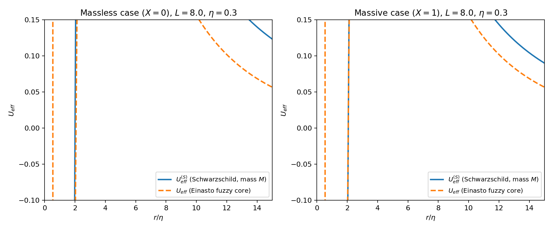
For a test particle of angular momentum (rescaled by the source’s Schwarzschild radius ) and (massive) or (massless), the radial geodesic equation takes the form of an energy-conservation relation const, with
| (17) |
Replacing (constant) recovers the Schwarzschild potential . In terms of , the Schwarzschild potential reads , whose extrema, obtained by solving directly, are the roots of ,
| (18) |
A fuzzy compact object built on the Einasto mass function mimics the Schwarzschild potential for bound-orbit physics provided has already saturated to by the radius , i.e. ; when this holds, and coincide closely not only at their minima but over a broad surrounding region, while differing sharply at small where the fuzzy core regularizes the potential (Fig. 5).
8 Non-local equation of state: self-gravitating droplets
As a second, independent closure of the anisotropic system, we replace the local de Sitter EOS with a non-local one,
| (19) |
motivated by the expectation that, for a diffuse density distribution, a local change in radial pressure should not depend solely on the local energy density but on the mass enclosed within the entire interior region. Evaluated exactly (Fig. 6), is positive near the core and turns negative for beyond a few , approaching zero from below as – since decays exponentially while falls off only as a power law once has largely saturated.
8.1 Field equations for the wormhole-type ansatz
This branch uses the more general static ansatz
| (20) |
with independent functions and . Its Ricci scalar is
| (21) |
and the Einstein-tensor components of Eq. (6) give
| (22) |
The anisotropic conservation equation for this ansatz is
| (23) |
and solving the middle relation of Eq. (22) for gives, exactly,
| (24) |
which closes the system: given and from Eqs. (1) and (19), Eqs. (23)–(24) determine uniquely, for a horizonless configuration (, so that everywhere and Eq. (24) has no pole). Both and are finite at (Fig. 6, right panel).

8.2 Curvature regularity: the Kretschmann scalar
The metric of Eq. (20) can be written, using , in wormhole-type form; its Kretschmann scalar , computed directly for independent , is exactly
| (25) |
Every term in Eq. (25) is manifestly finite as provided – guaranteed by any cored density profile with finite – and , the standard regularity condition for a static, non-singular interior. This confirms directly that the non-local-EOS droplet is free of a curvature singularity at the origin.
9 Testing the framework: alternative gravity model and alternative density profile
Because Eqs. (1)–(25) were derived and used generically – in terms of an arbitrary cored density profile , and (for the field equations) an arbitrary power in – the construction can be tested directly against two independent alternatives, holding everything else fixed.
9.1 A different curvature model: cubic gravity
Setting in Eq. (6) gives the same linear GR relation found for every , so the perturbative method of §5 applies unchanged, with a new (considerably longer, since cubic curvature brings in products of second derivatives) source functional . Evaluated on the identical Einasto droplet configuration used in §5, Fig. 7 shows that the cubic () correction has the opposite sign from the quadratic (Starobinsky) correction at the same , and a visibly different radial shape – more sharply peaked near the core and falling off faster. Both stay regular at and both relax back to the GR baseline at large . This is the central point of testing the gravity sector independently: the qualitative regularity story (finite core, GR exterior) is robust across models, but the sign and detailed shape of the near-core deformation is a genuine, model-dependent physical prediction, not something that can be inferred without repeating the calculation for each curvature model.

9.2 A different density profile: the Burkert halo
Holding and the de Sitter EOS fixed, we replace the Einasto profile with the Burkert profile, Eq. (4), and feed it through exactly the same , , , and formulas used for Einasto, with no other change. The core regularity mechanism is identical, since is again finite: the pressure profiles have the same qualitative shape as Fig. 1, and horizon formation again requires the central compactness to exceed a critical value.
What genuinely changes is the horizon structure at large (Fig. 8, centre panel, plotted on a logarithmic radial axis to display both horizons simultaneously). Because the Burkert mass function grows without bound as (logarithmically) rather than saturating to a finite total mass, once a horizon forms at all, two horizons still appear – an inner and outer , exactly as for Einasto – but they now sit at wildly different scales: for example, against for (in units where ), because the outer horizon only forms once the slowly-growing finally drops back below , rather than because the enclosed mass has converged. This is a genuine, physically meaningful difference between two comparably realistic dark-matter models: Einasto’s finite total mass keeps its double-horizon structure at a single characteristic scale (Fig. 2), while a profile without a finite total mass generically does not.

10 Discussion and conclusion
We have constructed regular, dark-matter-supported compact objects in a one-parameter family of curvature-corrected gravity theories, , working throughout with the empirically motivated Einasto DM density profile. In the exact limit, the interior solution is completely regular at the origin – a de Sitter core replaces the classical central singularity – and, depending on a single rescaled-mass parameter, describes either a horizonless self-gravitating droplet or a genuine black hole with one or two Killing horizons. We showed that the associated Hawking temperature is a non-monotonic function of horizon radius, vanishing at both the near-extremal and the dilute (large-horizon) limits, and that the resulting effective potential can be tuned to match the Schwarzschild potential of a comparable point mass away from the core, while remaining regular within it.
Treating the curvature parameter perturbatively, we obtained a closed-form integral solution for the leading-order correction to the metric function, valid for any power and any cored density profile – a genuine methodological generalization of the purely numerical treatments common in this literature. Applying this method to two distinct curvature models at fixed showed that the sign and detailed shape of the correction is model-dependent physics, testable in principle rather than universal. We repeated the entire construction, including a Kretschmann-scalar regularity check, for an independent non-local equation of state, and again found fully regular self-gravitating droplets. Finally, replacing the Einasto profile with the Burkert profile – holding every other assumption fixed – preserved the qualitative regularity mechanism but produced a horizon structure with a nearly three-orders-of-magnitude separation between inner and outer horizon radii, traced directly to the absence of a finite total halo mass in the Burkert model. This last result illustrates a broader point: the qualitative features of DM-supported regular compact objects (a de Sitter core, a well-defined horizon-formation threshold) are robust across reasonable choices of density profile and curvature model, but quantitative predictions – horizon radii, temperatures, the detailed shape of near-core curvature corrections – depend on those choices in ways that are only revealed by carrying the calculation through explicitly for each case, as we have done here for representative examples of both axes of variation.
Appendix A The (Starobinsky) field equations
For completeness, we record here the explicit projections of Eq. (6) for the illustrative case , obtained by direct substitution of , (Eq. (9)) and their derivatives:
| (26) | ||||
| (27) | ||||
| (28) |
Setting in Eqs. (26)–(28) recovers Eq. (13), as it must for every . This case was used to validate the general- symbolic derivation of §3 and to extract the source functional used in §5. The substantive analysis of this paper – the general- formalism, the closed-form perturbative method, the comparison, and the density-profile comparison – does not depend on this appendix.
References
- [1] (2017) The realistic models of relativistic stars in gravity. Class. Quantum Gravity 34, pp. 205008. Cited by: §1.
- [2] (1968) Non-singular general-relativistic gravitational collapse. In Proceedings of the International Conference GR5, Tbilisi, USSR. Cited by: §1.
- [3] (2018) History of dark matter. Rev. Mod. Phys. 90, pp. 045002. Cited by: §1.
- [4] (2019) A model for a dark matter core at the galactic centre. Monthly Notices of the Royal Astronomical Society 484 (3), pp. 3325–3333. Cited by: §1.
- [5] (1995) The structure of dark matter halos in dwarf galaxies. Astrophys. J. 447, pp. L25–L28. Cited by: §1, §1, §2.2.
- [6] (2011) Extended theories of gravity. Phys. Rep. 509, pp. 167–321. Cited by: §1.
- [7] (2010) Neutron stars in gravity with perturbative constraints. Phys. Rev. D 82, pp. 064033. Cited by: §1.
- [8] (2019) On the estimation of the local dark matter density using the rotation curve of the milky way. JCAP 2019, pp. 037. Cited by: §1.
- [9] (1992) Vacuum nonsingular black hole. Gen. Relativ. Gravit. 24, pp. 235–242. Cited by: §1.
- [10] (1969) On the construction of a composite model for the galaxy and on the determination of the system of galactic parameters. Astron. Nachr. 291, pp. 97–111. Cited by: §1.
- [11] (2012) Allgemeine relativitätstheorie. 6 edition, Springer. Cited by: §1.
- [12] (2020) Detection of the schwarzschild precession in the orbit of the star s2 near the galactic centre massive black hole. Astron. Astrophys. 636, pp. L5. Cited by: §1.
- [13] (2006) Formation and evaporation of nonsingular black holes. Phys. Rev. Lett. 96, pp. 031103. Cited by: §1.
- [14] (2007) Models of cosmic acceleration that evade solar-system tests. Phys. Rev. D 76, pp. 064004. Cited by: §1, §3.
- [15] (2024) Structure of anisotropic fuzzy dark matter black holes. Eur. Phys. J. C 84, pp. 572. External Links: Document Cited by: §1.
- [16] (1964) Relativistic equations for adiabatic, spherically symmetric gravitational collapse. Phys. Rev. 136, pp. B571–B576. External Links: Document Cited by: §2.1, §3.1.
- [17] (1996) The structure of cold dark matter halos. Astrophys. J. 462, pp. 563–575. Cited by: §1.
- [18] (2006) Noncommutative geometry inspired schwarzschild black hole. Phys. Lett. B 632, pp. 547–551. Cited by: §1.
- [19] (2009) Noncommutative black holes, the final appeal to quantum gravity: a review. Int. J. Mod. Phys. A 24, pp. 1229–1308. Cited by: §1.
- [20] (2012) Analytical properties of einasto dark matter haloes. Astron. Astrophys. 540, pp. A70. Cited by: §1.
- [21] (1966) Initial stage of an expanding universe and appearance of a nonuniform distribution of matter. Sov. Phys. JETP 22, pp. 241–249. Cited by: §1.
- [22] (2015) Radiating cylindrical gravitational collapse with structure scalars in gravity. Astrophysics and Space Science 357 (1), pp. 49. Cited by: §1.
- [23] (2010) Theories of gravity. Rev. Mod. Phys. 82, pp. 451–497. Cited by: §1.
- [24] (1980) A new type of isotropic cosmological models without singularity. Phys. Lett. B 91, pp. 99–102. Cited by: §1, §3.
- [25] (1996) Analytical models for galactic nuclei. Mon. Not. R. Astron. Soc. 278, pp. 488–496. Cited by: §1.