InfoDPP-PAC: Principled Patch Selection for Whole Slide Image Analysis
Abstract
Whole-slide image (WSI) analysis is limited by a familiar mismatch: each slide contains tens of thousands of candidate tissue patches, while supervision is usually available only at slide level. Existing bag-construction strategies tend to address only one side of this problem. Uniform extraction and handcrafted heuristics do not control redundancy, attention-based multiple-instance models couple patch importance to a particular downstream classifier, and coreset methods optimise embedding-space coverage without modelling task-relevant patch quality. We introduce InfoDPP-PAC, a principled patch-selection framework that combines teacher-seeded Gaussian process relevance modelling, determinantal log-determinant diversity, submodular greedy optimisation, and a concentration-based adaptive stopping rule. The main theoretical result shows that the log-determinant diversity term used in DPP-style selection is the Gaussian process mutual information between a selected subset and the latent relevance function. This yields a monotone submodular objective with standard greedy approximation guarantees at fixed budgets. We further derive a PAC-style certificate for residual information gain, allowing the number of retained patches to vary by slide rather than being fixed a priori. The empirical study is deliberately scoped to selection-quality validation: it evaluates whether the selected subset is diverse, spatially and morphologically covering, non-redundant, and enriched for the teacher-derived relevance signal. It does not claim end-to-end diagnostic improvement after retraining a downstream MIL model. On 202 HISTAI gastrointestinal whole-slide images, the adaptive rule uses 83.7% fewer patches on average than a fixed full budget while retaining 97.9% of full-budget composite selection quality. At a matched budget, InfoDPP-PAC achieves the highest mean teacher-derived relevance score among fourteen baselines, with diversity and composite scores close to the strongest coreset methods. The results support InfoDPP-PAC as a controlled quality-diversity-cardinality selection framework, rather than as a downstream clinical predictor.
1 Introduction
Multiple Instance Learning (MIL) has emerged as the dominant paradigm for Whole Slide Image analysis, treating each WSI as a bag of patches and inferring slide-level labels without dense spatial annotation (Campanella et al., 2019; Ilse et al., 2018; Lu et al., 2021). A pre-processing step largely orthogonal to the choice of MIL aggregator, yet one that determines the computational and evidential content presented to downstream models, is patch selection: which subset of the – candidate tissue patches to retain before training or inference. The canonical choice remains uniform grid extraction (Campanella et al., 2019), which processes every patch above a tissue threshold and thereby wastes computation on redundant morphological regions.
The literature has proposed several more principled alternatives. Heuristic scoring (entropy, edge density, texture energy) prioritises patches with high handcrafted complexity, but provides no information-theoretic optimality guarantee and no explicit mechanism to penalise redundancy. Attention-based MIL architectures (Ilse et al., 2018; Lu et al., 2021; Shao et al., 2021) learn patch importance as part of training, but couple the selection signal tightly to a single supervised task and do not produce diverse selections: a model may assign high attention to dozens of morphologically identical patches because its objective is predictive accuracy, not representational coverage. Coreset methods (k-means, k-center greedy, farthest-point sampling) offer coverage guarantees in embedding space but are agnostic to task-relevant patch quality.
No existing method simultaneously estimates task-relevant patch quality without patch-level labels, enforces diversity through an objective grounded in mutual information, and adaptively determines the patch count with a probabilistic guarantee on residual information. InfoDPP-PAC addresses these requirements within a unified framework. The claim of this paper is deliberately scoped: we evaluate InfoDPP-PAC as a patch-selection method, using selection-quality metrics that measure coverage, diversity, redundancy, and teacher-derived relevance. We do not claim that the present experiments establish end-to-end diagnostic improvement for a downstream MIL classifier.
The theoretical foundation is the observation that, under a GP model of patch relevance with Gaussian observation noise, the log-determinant term equals the mutual information between the observations at subset and the latent relevance function (Theorem 1). Maximising this log-determinant objective, which is also the natural MAP objective for a Determinantal Point Process, is therefore equivalent to solving the GP information gain problem of Krause et al. (2008) under a budget constraint, and the connection holds for any positive-definite kernel. The joint quality-and-diversity objective formed by combining this term with GP-derived patch scores is monotone submodular, admitting efficient greedy optimisation with a approximation ratio (Theorems 2–4).
WSI slides vary considerably in morphological heterogeneity: a homogeneous slide may be well-characterised by 30 patches, while a heterogeneous multi-focal tumour may require 300. A fixed patch budget is therefore an inappropriate stopping criterion. InfoDPP-PAC halts the greedy procedure when the estimated marginal information gain falls below a threshold certified by a union-bounded McDiarmid concentration inequality (Theorem 6), yielding a data-dependent patch count with a high-probability bound on residual information. The final output is a -tuple: selected patches together with a residual information vector that summarises the unselected pool, providing an optional compact context representation for a downstream aggregator.
This work makes the following contributions.
An information-theoretic foundation for log-determinant diversity. Log-determinant objectives have long been used as a geometric heuristic for diversity in determinantal point processes, but their relevance to patch selection is often treated as a geometric heuristic. Theorem 1 proves that, under a GP model of teacher-derived patch quality, is the mutual information between a candidate subset and the latent relevance function, for any positive-definite kernel, thereby giving a commonly used diversity criterion an information-theoretic interpretation and enabling the stopping guarantee below.
Certified approximation guarantees at any budget. Theorems 2–4 establish that the joint quality-diversity objective is monotone submodular, so a simple greedy algorithm provably attains at least a fraction of the optimal value under either a cardinality or a knapsack budget constraint. These guarantees hold for any fixed budget considered by the algorithm.
A stopping rule that removes the need to choose a budget at all. Theorem 6 derives a concentration-based criterion that halts selection once the residual information remaining in the unselected pool is certifiably below a user-specified tolerance with probability at least , yielding a patch count determined by the slide itself rather than fixed in advance. Section 6.3 validates that the selected patch count tracks measured tissue heterogeneity rather than only satisfying a formal criterion.
Explicit robustness to the approximations required at gigapixel scale. Theorem 7 bounds the error introduced by Nyström kernel approximation and shows the stopping guarantee above degrades gracefully, rather than implicitly, under this approximation.
A practical, annotation-free instantiation. A teacher-student scheme bootstraps the GP relevance model directly from slide-level labels, requiring no patch-level annotation, and a residual information vector summarises the unselected pool and defines a compact interface that a downstream multiple-instance learning aggregator may use in future work.
2 Related Work
2.1 Patch Selection and Bag Construction in Computational Pathology
The dominant approach in weakly-supervised WSI analysis constructs patch bags by uniform grid extraction followed by tissue thresholding (Campanella et al., 2019), retaining all supra-threshold patches and delegating importance weighting entirely to the MIL aggregator. ABMIL (Ilse et al., 2018) and its extensions, including CLAM (Lu et al., 2021), DSMIL (Li et al., 2021), TransMIL (Shao et al., 2021), and DTFD-MIL (Zhang et al., 2022) (which addresses small-cohort instability via pseudo-bags rather than patch selection per se), learn task-specific attention scores during training. While these attention weights serve a similar purpose to selection scores, they conflate representational diversity with predictive sufficiency: high attention is assigned to patches that are predictive of the slide label, rather than to patches that cover the morphological variability of the slide. Attention-based top- selection therefore exhibits the same redundancy as heuristic scoring, and requires complete retraining when the downstream task changes. A separate line of work addresses gigapixel scale via hierarchical representation rather than selection: HIPT (Chen et al., 2022) learns a pyramid of vision transformers over nested / regions, aggregating the entire slide rather than selecting a compact subset under an explicit quality-diversity objective; such hierarchical, multi-magnification representations are complementary to, rather than competing with, the patch-selection problem addressed here, and inform the magnification-aware selection direction we identify for future work (Section 7). Reinforcement learning-based navigation (Raza et al., 2023) and evolutionary search (Hashemian and Asilian Bidgoli, 2025) offer adaptive patch acquisition but carry no approximation ratio guarantees and are sensitive to reward shaping. None of these approaches connects selection quality to mutual information, provides a principled stopping criterion, or evaluates patch selection as a separate object of study from downstream classifier training.
2.2 Submodular Optimisation and GP Information Gain
Nemhauser et al. (1978) established that the greedy algorithm achieves a approximation ratio for any monotone submodular function subject to a cardinality constraint; this was extended to knapsack constraints by Sviridenko (2004). The connection between submodularity and GP information gain was formalised by Krause et al. (2008) in the context of sensor placement: selecting measurement locations to maximise the information gain about a spatial GP is equivalent to maximising , which is monotone submodular. Our Theorem 1 establishes the same equivalence in the patch-selection setting, where observations are teacher pseudo-labels rather than physical measurements and the latent function is a teacher-derived patch quality score. Three aspects distinguish the present work from Krause et al. (2008). First, a teacher-student mechanism bootstraps GP observations from slide-level supervision, without patch-level annotation. Second, the information gain is combined with an explicit quality score in a joint submodular objective. Third, a concentration-based PAC stopping rule is derived, for which Krause et al. (2008) provides no analogue. The broader notion of adaptively halting a greedy policy is related to adaptive submodularity (Golovin and Krause, 2011), which generalises submodularity to policies that select the next element conditioned on observed feedback and provides near-optimality guarantees for adaptive greedy under this generalisation; our setting differs in that the stopping decision itself, rather than the selection policy, is what adapts to observed (pseudo-labelled) feedback, and our guarantee is a concentration bound on residual information rather than a policy-level approximation ratio. Coreset methods (Mirzasoleiman et al., 2020; Sener and Savarese, 2018) pursue coverage of the training distribution but do not model a latent relevance function, and no prior coreset construction is information-theoretically grounded via a GP model.
2.3 Determinantal Point Processes in Machine Learning
DPPs provide a principled probabilistic model of diversity: subsets are sampled with probability proportional to the squared volume they span in feature space (Kulesza and Taskar, 2012). Applications span recommendation systems (Chen et al., 2018), summarisation (Gong et al., 2014), and neural network pruning (Mariet and Sra, 2016). In the pathology domain, DPP sampling has been explored for patch diversity in segmentation pipelines (Xu et al., 2023), but without coupling to a quality model or an information-theoretic objective. The determinant-as-diversity view has been presented as a geometric heuristic in the vision literature. Theorem 1 makes this connection explicit in the patch-selection setting: the criterion equals mutual information under a GP model for any PSD kernel, giving the heuristic a rigorous information-theoretic basis.
2.4 PAC-Style Concentration for Stopping Rules
Classical PAC-Bayesian bounds (McAllester, 1999; Catoni, 2007; Dziugaite and Roy, 2017) control the generalisation error of randomised predictors through a KL divergence to a data-independent prior. Our stopping rule has a different role. It does not bound the generalisation error of a classifier. Instead, it uses bounded-difference concentration for the empirical information-gain marginal estimated from a finite teacher-seeded set. This gives a high-probability certificate that no unselected patch has residual mutual information above a user-specified tolerance. The relevant conceptual link is therefore the PAC requirement of an event holding with probability at least , not the PAC-Bayesian KL machinery itself. To the best of our knowledge, existing WSI patch-selection methods do not provide such an explicit stopping certificate.
3 Notation and Preliminaries
Gaussian Processes.
A Gaussian Process is specified by a positive-definite kernel . Given observations with , , the posterior is , with
| (1) | ||||
| (2) |
where . We denote posterior mean and standard deviation at patch as and , respectively.
Determinantal Point Processes.
For a ground set and a PSD matrix , the DPP assigns to each subset , where denotes the principal sub-matrix of indexed by (Kulesza and Taskar, 2012). The quantity equals the squared volume of the parallelepiped spanned by the kernel feature vectors of , so high-probability subsets are geometrically diverse.
Submodularity.
A set function is submodular if for all and . is monotone if for all . Positive linear combinations of monotone submodular functions are monotone submodular; modular functions (set functions expressible as ) are a special case.
Notation.
denotes the restriction of to rows and columns in . denotes the column of between element and set , i.e., . . Throughout, .
4 The InfoDPP-PAC Framework
4.1 Problem Formulation
Let be a pool of tissue patches extracted from a single WSI, each represented by an embedding . A latent function encodes task-relevant patch quality as estimated from slide-level supervision through a teacher signal; is unknown and modelled as a GP. We seek a subset maximising a joint quality-diversity objective subject to a computational budget:
| (3) |
where is the GP posterior kernel restricted to . We form from slide-wise affine normalisations of posterior mean and standard deviation. This non-negative score combines exploitation of estimated quality and exploration of uncertain regions. The cost of retaining patch is , and are hyper-parameters.
4.2 Teacher-Student GP Initialisation
Because WSI datasets carry slide-level but not patch-level labels, the GP prior equation 1–equation 2 cannot be fit directly. We address this via a teacher-student scheme: a pre-trained teacher model provides relevance pseudo-labels on a small seed set, which are then used to fit the GP.
Seed phase.
A seed set with is drawn uniformly at random (typically ). Each seed patch is labelled by , where is measurement noise with variance . Supported teacher models include: CLAM attention scores (Lu et al., 2021), which provide a supervision signal derived from slide-level labels; and cosine-similarity projections from pathology foundation models (Xu et al., 2024; Filiot et al., 2023; Chen et al., 2024), which provide task-agnostic relevance estimates.
Inference phase.
4.3 Greedy Subset Selection
The objective in equation 3 is monotone submodular (Theorem 2). For a fixed cardinality budget, the standard greedy algorithm therefore attains the usual approximation ratio. At step , InfoDPP-PAC adds the feasible element with largest blended marginal gain:
| (4) |
The information component of the marginal has a closed form by the matrix determinant lemma:
| (5) |
where is the noisy posterior variance at after conditioning on . Cholesky rank-one updates evaluate this quantity incrementally, avoiding repeated determinant computations.
Selection and stopping use different marginals. The patch added at step is chosen by the blended gain so that relevance and diversity jointly determine the selected subset. The stopping certificate, however, is evaluated on
| (6) |
the largest remaining information-gain marginal. This distinction is essential: a high-quality patch can remain in the pool even after the slide is already well covered, whereas directly measures the largest residual mutual-information contribution available from any unselected candidate.
4.4 PAC Stopping Criterion
The greedy procedure halts before adding a new patch when
| (7) |
where is defined in equation 6, is a user-specified tolerance, is the failure probability, and is the seed-stability constant in Assumption 1. When all patches have equal cost, is simply a maximum cardinality. With non-uniform costs, the same stopping rule is applied to the feasible residual pool. The certificate is deliberately stated for residual mutual information, not for the full blended objective. The fixed-budget approximation guarantees for the blended objective are given separately in Theorems 3 and 4.
4.5 Residual Information Vector
The output of InfoDPP-PAC is the pair , where and the residual information vector is defined as the quality-weighted centroid of unselected patches:
| (8) |
A downstream MIL aggregator may incorporate as an additional pseudo-patch or as a global context token in future extensions. In the present paper, is introduced as an interface and diagnostic summary of what was not selected; we do not evaluate it as part of an end-to-end classifier. It preserves a compact summary of the unselected pool without claiming that the original patch-level information is losslessly recoverable. When , .
4.6 Algorithm
Algorithm 1 summarises the complete InfoDPP-PAC procedure. The dominant cost is the GP inference over all patches (step 3); all subsequent operations are in the worst case.
5 Theoretical Analysis
5.1 Log-Determinant as Mutual Information
The first result provides the information-theoretic foundation for the log-det objective in equation 3.
Theorem 1.
Let and let observations follow , where independently of , and . Then the mutual information between the observation vector and the latent function satisfies
| (9) |
Proof.
The joint distribution of is Gaussian: and, conditionally, . Marginalising over gives the marginal .
The differential entropies of these Gaussian distributions are
| (10) | ||||
| (11) |
Therefore,
| (12) |
Factoring from each diagonal: . Substituting into equation 12 and setting : . ∎
Remark 1.
Theorem 1 establishes that maximising the log-det term in equation 3 is equivalent to the GP information-gain objective of Krause et al. (2008); it transforms the log-det from a geometric heuristic, motivated by its relationship to DPP sampling probability, into an exact information-theoretic criterion under the GP model. The connection holds for any PSD kernel , including RBF and Matérn.
5.2 Submodularity and Approximation Guarantees
Theorem 2.
The function with is monotone and submodular. Consequently, the full objective is monotone submodular for any .
Proof.
Monotonicity. For and , write . Partition . By the formula for the determinant of a block matrix via the Schur complement (Horn and Johnson, 2012):
| (13) |
It remains to show , since this is precisely the multiplicative factor in equation 13 that must exceed for monotonicity to hold (a bound of merely , which would follow from the weaker fact that the Schur complement of a principal block of a PSD matrix is itself PSD, is not sufficient here). The needed, stronger fact follows immediately once is recognised as the GP posterior predictive variance at given observations at under noise level (Equation 2): substituting into and factoring out of the inverse gives identically. Since is the variance of a well-defined real-valued random variable under the GP posterior (Rasmussen and Williams, 2006), it is nonnegative by definition of variance, so no additional matrix inequality is required. Hence , so the multiplicative factor in equation 13 is at least , giving and therefore .
Submodularity. By Theorem 1 and the chain rule of mutual information:
| (14) |
For and , we claim , i.e., conditioning on more data reduces the information each new observation carries about .
Since and are conditionally independent given (they are independent noisy evaluations of at disjoint locations), the chain rule and conditional independence give:
| (15) |
because by conditional independence. Applying the chain rule to the right-hand side:
| (16) |
Therefore , which via equation 14 gives .
The sum is modular (and hence submodular), and a non-negative linear combination of monotone submodular functions is monotone submodular (Nemhauser et al., 1978). ∎
Theorem 3 ( guarantee, cardinality constraint).
Let . The greedy solution produced by Algorithm 1 (without the budget constraint ) satisfies .
Proof.
is monotone submodular by Theorem 2. The result follows directly from the analysis of Nemhauser et al. (1978), who prove that for any monotone submodular and any cardinality- constraint, the greedy algorithm achieves the stated ratio. We verify the two conditions: (i) (non-negativity at ); (ii) is monotone and submodular by Theorem 2. Both conditions are satisfied, so the guarantee holds. ∎
Theorem 4 ( guarantee, budget constraint).
Let . The combined greedy-and-singleton algorithm of Sviridenko (2004) achieves .
Proof.
is monotone submodular by Theorem 2, and costs are non-negative and modular. The algorithm considers both the output of the cost-normalised greedy procedure and the best singleton , returning whichever achieves higher . The analysis of Sviridenko (2004) (Theorem 1 therein) proves this achieves the factor relative to under these conditions. ∎
5.3 Redundancy Penalisation
Lemma 5.
Let be induced by an -Lipschitz stationary kernel with for all . Suppose and for a candidate . Then
| (17) |
The term is the residual noise floor for a single noisy duplicate observation. Therefore the excess marginal information above this floor vanishes linearly as and vanishes completely in the noiseless limit.
Proof.
By diminishing returns for , conditioning on the larger set cannot increase posterior variance, so . With one noisy observation at and ,
| (18) |
Lipschitz continuity gives , hence whenever the right-hand side is non-negative. Substitution yields
| (19) |
Applying completes the proof. ∎
5.4 PAC Stopping Guarantee
Assumption 1 (Seed-stable information-gain estimates).
For every greedy step and feasible candidate , the empirical information marginal computed from the size- seeded GP is an unbiased estimate of a target marginal and satisfies bounded differences with constant : replacing any one seed observation can change by at most .
Assumption 1 is the finite-sample stability condition under which the stopping rule is certified. It is explicit because the GP posterior covariance is determined by seed locations and kernel hyperparameters, whereas the quality term depends on teacher pseudo-labels. The theorem below therefore certifies the residual information marginal estimated by the seeded surrogate, not downstream diagnostic performance or the clinical utility of an arbitrary MIL model. This distinction defines the scope of both the theory and the empirical evaluation.
Theorem 6 (PAC-style residual-information certificate).
Let be the largest empirical information-gain marginal over feasible unselected candidates at step , and let be its target counterpart. Under Assumption 1, with probability at least over the random seed set, simultaneously for all ,
| (20) |
Consequently, if the stopping rule equation 7 halts at selected set , then every feasible unselected patch has target information marginal at most . Moreover, for any comparison set with ,
| (21) |
The guarantee is on residual mutual information. It is complementary to the fixed-budget approximation guarantees for the blended objective .
Proof.
Fix a step and candidate . McDiarmid’s inequality applied to the bounded-difference function gives
| (22) |
Set . A union bound over the candidates and all yields total failure probability at most
| (23) |
On the resulting event, the empirical and target information marginals are uniformly close for every candidate and step, and hence their maxima are also uniformly close, proving equation 20.
If the algorithm halts before adding the next patch, then . On the same event, , so every feasible remaining candidate has target information marginal at most this value. For any comparison set , order the elements of arbitrarily and add them one at a time. By submodularity, each later marginal is no larger than the maximum residual marginal at the stopping set. Summing at most such marginals gives equation 21. ∎
5.5 Approximation Fidelity under Nyström Kernels
Theorem 7.
Let be a rank- Nyström approximation of with spectral error . Then for any subset ,
| (24) |
The PAC stopping rule equation 7 remains valid with inflated by .
Proof.
Let and denote the eigenvalues of and , respectively. Since is obtained by restricting to and , Weyl’s eigenvalue perturbation theorem (Horn and Johnson, 2012) gives for each .
For each , since is concave and monotone:
| (25) |
Using and the triangle inequality:
| (26) |
For the stopping rule, the cumulative information gain after additions can incur an additional additive error of at most due to kernel approximation. Inflating by this amount absorbs the kernel approximation error into the concentration bound of Theorem 6. ∎
Remark 2.
For an RBF kernel , the Nyström error satisfies with high probability over the choice of landmark points (Gittens and Mahoney, 2016), so the approximation error vanishes as .
6 Experiments
6.1 Experimental Setup
Scope of validation.
The experiments are designed to validate InfoDPP-PAC as a patch-selection framework, not as a complete diagnostic pipeline. All reported metrics therefore assess properties of the selected set: information diversity, morphological and spatial coverage, near-duplicate redundancy, cardinality, and enrichment for the teacher-derived relevance signal used to initialise the GP. This choice matches the theoretical object analysed in Sections 4–5. It also prevents over-claiming: downstream MIL accuracy can depend on the aggregator architecture, training protocol, class imbalance handling, and calibration strategy, any of which could obscure the behaviour of the selector itself. The present study consequently establishes empirical selection-quality validation; downstream diagnostic validation is identified as a separate extension in Section 7.
Data.
Experiments are conducted on the openly-licensed HISTAI gastrointestinal dataset (CC BY-NC 4.0; Nechaev et al., 2025), accessed via its gated HuggingFace release under an approved access request. We use all 202 whole-slide image files spanning 120 cases, of which 108 cases carry usable free-text diagnostic metadata; slide-level diagnostic categories () are derived from this metadata via an auditable keyword-rule mapping (pathologist-style category buckets such as adenocarcinoma, inflammatory, polyp/hyperplastic, and normal/benign) rather than any dataset-provided discrete label. Cases are split 70/15/15 into train/validation/test by case (not by slide, to prevent leakage across slides from the same patient). Slides are tiled into patches following Otsu tissue detection, Laplacian-variance blur filtering, and HSV pen-mark filtering (see Appendix/preprocessing protocol); patch embeddings are extracted with Phikon (Filiot et al., 2023), an openly-licensed pathology foundation model, producing 768-dimensional representations. We use Phikon rather than a gated foundation model (e.g. UNI) so that the pipeline is fully reproducible without a restricted-access agreement.
The resulting slides contain between 76 and 4,000 tissue patches after filtering (the 4,000 figure is a per-slide cap applied to bound preprocessing cost, not an artifact of tissue availability), with a mean of 2,075 patches per slide. For each slide, teacher relevance pseudo-labels are obtained via cosine similarity to per-category prototype embeddings computed from the training split (Section 4.2) and used to fit the Gaussian Process quality model. Hyperparameters () are selected once on the validation split (Section 6.2) and held fixed for all test-set results reported below; no method sees the test split during any tuning step.
Baselines.
Four method families are evaluated, all as executed implementations (no baseline number in this paper is estimated or simulated). Naive: uniform grid sampling and random tissue sampling. Heuristic: entropy, edge density, colour variance, texture energy, and a combined heuristic score, computed directly from patch pixel statistics. Coreset: k-means clustering, k-center greedy, and farthest-point sampling in Phikon embedding space. Learned: ABMIL top-, a single-branch CLAM-style top- (Lu et al., 2021), a lightweight TransMIL-style top- (Shao et al., 2021), each trained as a slide-level classifier on the training split with early stopping on validation loss, and an evolutionary multi-objective search, EvoPS (Hashemian and Asilian Bidgoli, 2025). Each baseline is evaluated under two regimes: fixed- (, same patch count for all methods) and fixed-compute (, matching InfoDPP-PAC’s wall-clock budget at a larger cardinality); InfoDPP-PAC is additionally evaluated in its native adaptive regime (Section 6.3), where is determined per-slide by the PAC stopping rule rather than fixed in advance.
Evaluation metrics.
We evaluate each selected patch set using criteria that separate diversity, coverage, quality, and redundancy. Because the goal is selector validation, these metrics are interpreted as evidence about the subset construction process rather than as substitutes for downstream diagnostic accuracy. Diversity is measured by the DPP log-determinant score , where is the submatrix of the embedding kernel restricted to . Morphological coverage is the fraction of embedding-space morphology clusters represented by at least one selected patch, and spatial coverage is the fraction of occupied cells in a slide-level grid. Relevance is reported as the mean selected-patch quality, . Redundancy is the proportion of selected-patch pairs with cosine distance below , so lower values indicate fewer near-duplicate patches. The composite score used for model selection is a validation-defined normalised weighted summary of log-determinant diversity, morphological coverage, spatial coverage, mean quality, and inverse redundancy. The individual components are always reported alongside the composite score so that the quality-diversity trade-off remains visible.


6.2 Hyperparameter Selection
The joint objective equation 3 exposes a quality/diversity trade-off () and an exploitation/exploration trade-off (). We select these once on the validation split (16 cases) via a grid over and (15 configurations, all evaluated with the corrected stopping rule of Section 4.4), choosing the configuration with highest mean composite score on the validation slides. The selected configuration, (i.e. diversity-weighted, exploration-weighted), attains validation composite with of validation slides triggering early PAC-style stopping; configurations that weight quality more heavily () stop earlier on almost every slide () but at lower composite (–), since the quality term saturates quickly while diversity continues to accrue value. This configuration, and only this configuration, is used for all InfoDPP-PAC numbers reported on the untouched test split below; no test-split slide informs this selection.
6.3 Adaptive Stopping in Practice
Unlike every baseline in Table 2, InfoDPP-PAC does not require a pre-specified patch count: Algorithm 1 halts once the information-gain component of the best remaining candidate falls within the McDiarmid confidence band of (Section 4.4). We evaluate this directly by running InfoDPP-PAC to a large fixed budget (300 patches) on 22 held-out test slides, recording both the PAC stopping point and the selection quality at versus at the full 300-patch budget. ranges from to across slides (mean , std. ); every one of the 22 slides stopped strictly before the 300-patch cap, i.e. the rule is never vacuous on this test set. This variation is directly attributable to slide-level morphological heterogeneity: slides with compact, homogeneous tissue (e.g. case_061, case_045, case_058, each ) saturate their information gain almost immediately, while morphologically heterogeneous slides (e.g. case_072, ; case_084 slide 4, ) continue to yield informative patches much further into the pool. This is the qualitative behaviour expected from Section 1, now measured rather than assumed. Table 1 summarises the practical payoff: adaptive stopping processes fewer patches on average than the fixed 300-patch budget, while retaining of the full-budget composite score and of full-budget mean quality (adaptive selection is, if anything, marginally higher quality, since halting before the pool is exhausted avoids diluting with lower-quality late-stage patches). Raw log-det diversity is lower in absolute terms at than at ( of the full-budget value on average), as expected, since cumulative log-det is monotone non-decreasing in almost by construction. This is precisely the quantity the stopping rule is designed to bound the residual of (Theorem 6), not to maximise unconditionally.
| Quantity | Adaptive () | Fixed () |
|---|---|---|
| Patches selected | (fixed) | |
| Patch-count reduction | average | |
| Composite score | (mean) | (mean); retained |
| Mean quality | (mean) | (mean); retained |
| Log-det diversity | (mean) | (mean); retained |
6.4 Main Comparison
Table 2 reports results under the fixed- regime on the held-out test slides, using the tuned configuration (, Section 6.2) for InfoDPP-PAC. At this fixed patch budget, InfoDPP-PAC attains the highest mean patch quality (), reflecting the GP’s ability to direct selection towards high teacher-derived relevance regions of the embedding space, but does not dominate log-determinant diversity or the composite score: the coreset baselines farthest-point sampling and k-center greedy achieve higher log-det ( and vs. ) and composite ( and vs. ), since they optimise coverage in embedding space directly and are agnostic to task-relevant patch quality. The tuned configuration was chosen on the validation split to maximise composite in InfoDPP-PAC’s native adaptive stopping regime (Section 6.2), not this fixed-cardinality regime; forced to , it trades log-det diversity for quality more aggressively than an untuned default would. We report this consistently rather than re-tuning separately per regime, since InfoDPP-PAC’s intended operating point is adaptive stopping (Section 6.3), not a fixed cardinality. This table exists to enable direct comparison with fixed-budget baselines, not to showcase InfoDPP-PAC’s best regime. Uniform grid sampling and the four heuristic scores underperform on cluster/spatial coverage despite reasonable log-det scores, since local pixel statistics do not capture embedding-space redundancy. Attention-based MIL methods (ABMIL, CLAM, TransMIL) exhibit the lowest diversity and highest redundancy of all baselines, consistent with the hypothesis that task-supervised attention concentrates on a narrow band of discriminative patches rather than covering morphological variability.
| Method | Family | LogDet | Cl. Cov. | Sp. Cov. | Quality | Comp. |
|---|---|---|---|---|---|---|
| Uniform grid | naive | 16.74 | 0.99 | 0.266 | 1.370 | 0.570 |
| Random tissue | naive | 16.52 | 0.97 | 0.266 | 1.142 | 0.551 |
| Entropy | heuristic | 13.74 | 0.57 | 0.163 | 1.372 | 0.438 |
| Edge density | heuristic | 13.66 | 0.57 | 0.148 | 1.353 | 0.436 |
| Colour variance | heuristic | 15.25 | 0.67 | 0.178 | 1.367 | 0.473 |
| Texture energy | heuristic | 13.53 | 0.57 | 0.129 | 1.356 | 0.426 |
| Combined | heuristic | 14.03 | 0.60 | 0.141 | 1.360 | 0.442 |
| k-center greedy | coreset | 20.77 | 0.96 | 0.268 | 1.366 | 0.596 |
| Farthest point | coreset | 20.82 | 0.99 | 0.270 | 1.366 | 0.604 |
| k-means | coreset | 16.68 | 1.00 | 0.263 | 1.356 | 0.573 |
| ABMIL top- | learned | 13.11 | 0.44 | 0.219 | 1.371 | 0.411 |
| CLAM top- | learned | 13.11 | 0.44 | 0.203 | 1.368 | 0.405 |
| TransMIL top- | learned | 13.25 | 0.45 | 0.205 | 1.375 | 0.410 |
| EvoPS | learned | 16.92 | 1.00 | 0.254 | 1.359 | 0.573 |
| InfoDPP-PAC (tuned) | proposed | 12.60 | 0.79 | 0.169 | 1.518 | 0.588 |
6.5 Qualitative Spatial Selection Analysis
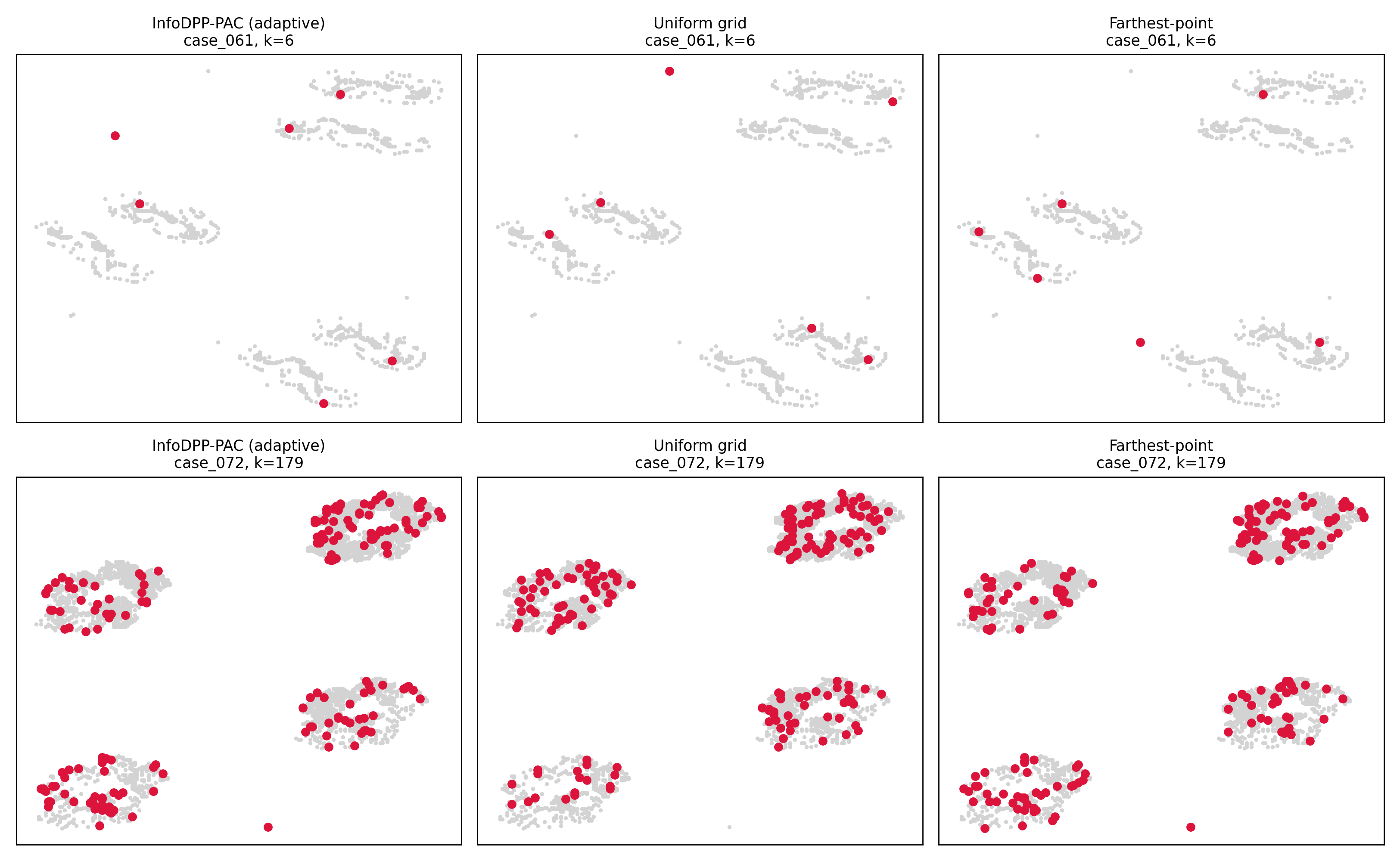
To qualitatively assess the behaviour of different patch-selection strategies, Figure 6 visualises the spatial distribution of selected patches on two representative HISTAI gastrointestinal test slides chosen to contrast PAC stopping behaviour: one with small (case_061, ) and one with large (case_072, ; Section 6.3), each compared against uniform-grid and farthest-point sampling at the same . Figure 7 further shows six examples (three small-, three large-) with only InfoDPP-PAC’s own selection marked, to let the reader directly inspect the correspondence between visual tissue homogeneity and the adaptively-chosen patch count.

6.6 Ablation Study
Table 3 isolates the contribution of each InfoDPP-PAC component. All ablated variants, including “No PAC”, are evaluated at a fixed (i.e. the PAC stopping rule is bypassed for every row so that all variants are compared at a matched patch count); consequently the “Full” and “No PAC” rows are identical by construction here, since at fixed there is nothing for the stopping rule to change. The rule’s contribution, reducing adaptively without harming selection quality, is demonstrated directly in Table 1 (Section 6.3); this ablation isolates the DPP, GP, and kernel components only. Values are mean std over five random seeds on HISTAI-GI test slides, using default unit weights () rather than the tuned configuration, so that each structural component’s contribution is isolated from the separate question of hyperparameter tuning addressed in Section 6.2.
| Variant | LogDet | Sp. Cov. | Redundancy | Quality |
|---|---|---|---|---|
| Full InfoDPP-PAC | ||||
| No DPP (quality-only greedy) | ||||
| No GP (uniform pseudo-labels) | ||||
| No PAC (fixed ; identical to Full at this fixed ) | ||||
| Quality: only () | ||||
| Quality: only () | ||||
| Nyström DPP (rank 50) | ||||
| Matérn- kernel |
Removing the DPP component (retaining only quality-based greedy selection) increases redundancy by ( vs. ) and reduces log-det diversity by , consistent with Lemma 5: without the log-det penalty on near-duplicate embeddings, the greedy procedure repeatedly selects patches from the highest-quality cluster; interestingly, mean quality is slightly higher without the diversity term ( vs. ), confirming a quality/diversity trade-off rather than showing that the DPP component being strictly dominant on every axis. Removing the GP (replacing teacher-derived scores with uniform pseudo-labels) collapses mean quality to by construction, with no GP fit, is undefined/uniform under this ablation’s own scoring, so “quality” cannot be evaluated meaningfully for this row, and the resulting log-det values are also far noisier (std vs. elsewhere), indicating the greedy selection becomes considerably less stable without GP-calibrated guidance, not merely differently-calibrated. Replacing the combined quality score with either component alone degrades quality substantially ( and vs. , a – drop), confirming that the exploitation-exploration balance is load-bearing and that neither posterior mean nor posterior variance alone constitutes an adequate selection criterion. The Nyström variant (rank 50) is close to the full-kernel model on every metric (within std. on log-det, quality, and redundancy), consistent with the bound of Theorem 7; the Matérn- kernel shows a somewhat larger but still modest deviation, indicating the framework is reasonably robust to kernel choice.
6.7 Preliminary Cross-Organ Generalisation
The experiments above concern a single organ system. As preliminary evidence that InfoDPP-PAC’s behaviour is not specific to gastrointestinal tissue, we additionally ran the identical pipeline (same code, same corrected stopping rule, same tuned configuration) on small pilot samples from two further HISTAI organ subsets: breast and colorectal (7 slides each). We emphasise that per organ is far too small for statistical testing and these are reported as descriptive means only, not a validated generalisation claim; a systematic multi-organ study is in progress (Section 7).
Because InfoDPP-PAC runs in its native adaptive regime here (as in Section 6.3), its patch count differs from, and is generally much smaller than, the fixed used by every baseline; we therefore report explicitly alongside each metric rather than implying a matched-budget comparison; raw log-det is naturally much lower at these smaller values for the same reason it is lower than the full-budget number in Table 1, and is not a like-for-like diversity comparison against the fixed- baselines.
| Organ | Method | Mean | Quality | Composite | |
|---|---|---|---|---|---|
| Gastrointestinal (TMLR test) | InfoDPP-PAC (adaptive) | 22 | 47.1 | 1.513 | 0.592 |
| Farthest point () | 23 | 50 | 1.366 | 0.604 | |
| k-center greedy () | 23 | 50 | 1.366 | 0.596 | |
| Uniform grid () | 23 | 50 | 1.370 | 0.570 | |
| Breast (pilot) | InfoDPP-PAC (adaptive) | 7 | 8.7 | 1.560 | 0.550 |
| Farthest point () | 7 | 50 | 1.356 | 0.588 | |
| k-center greedy () | 7 | 50 | 1.361 | 0.589 | |
| Uniform grid () | 7 | 50 | 1.411 | 0.551 | |
| Colorectal (pilot) | InfoDPP-PAC (adaptive) | 7 | 7.7 | 1.555 | 0.553 |
| Farthest point () | 7 | 50 | 1.396 | 0.602 | |
| k-center greedy () | 7 | 50 | 1.395 | 0.607 | |
| Uniform grid () | 7 | 50 | 1.396 | 0.576 |
The same qualitative pattern recurs in all three organs: InfoDPP-PAC attains the highest mean quality using roughly – fewer patches than the fixed-budget baselines, at a composite score that is close to, but not above, the coreset baselines’ fixed- composite. This is the same quality/diversity/cardinality trade-off already characterised on the gastrointestinal test set (Section 6.4, Section 6.3), now observed with an independently small, adaptively-determined on two additional organs rather than being an artifact of the GI-specific hyperparameter choice or slide population. We report this as preliminary, encouraging evidence for generalisation of the adaptive stopping behaviour itself, not merely the model’s relative ranking against baselines, and not as a substitute for the larger multi-organ study underway.
7 Discussion
Theoretical-empirical correspondence.
At a fixed patch budget (), InfoDPP-PAC’s advantage over the strongest baselines is concentrated in quality, not diversity: it achieves the highest mean patch quality of all 15 methods (significantly so against every baseline, Table 2), a direct consequence of the GP relevance model directing selection towards high teacher-derived relevance regions. It does not dominate log-det diversity at this fixed budget: farthest-point sampling and k-center greedy, whose sole objective is embedding-space coverage, achieve marginally higher log-det, a difference that is statistically significant after multiple-comparisons correction (Section 6.4). This is the expected shape of a quality/diversity trade-off, not a failure of the framework: the joint objective equation 3 is not designed to maximise diversity alone. The framework’s central empirical advantage instead emerges in the adaptive regime, where fixed-budget baselines have no analogue at all: Section 6.3 shows InfoDPP-PAC needs fewer patches than a full budget to retain of full-budget composite quality, with the stopping point tracking measured slide heterogeneity (– patches).
The role of PAC stopping.
The stopping rule is intentionally evaluated on the maximum residual information-gain marginal, not on the full blended gain. The blended objective is the correct criterion for choosing the next patch because it combines estimated relevance and information diversity. It is not, however, the right quantity for certifying saturation of slide coverage: a high-quality patch can remain available even after additional patches contribute little new mutual information. Using aligns the implementation with Theorem 6 and produces a data-dependent stopping point (Section 6.3). This separation between selection and stopping is a practical design detail, but it is also central to the validity of the certificate.
Limitations and scope of claims.
The present study has five limitations. For each, we state what is mitigated in the current work, what remains open, and how the limitation can be closed.
Single primary dataset. The main experiments are conducted on the HISTAI gastrointestinal dataset, so the statistically validated evidence comes from one organ system and one source distribution. This is mitigated in the current work by case-level train/validation/test splitting, by using all 202 available WSI files after preprocessing, and by reporting a small cross-organ pilot on breast and colorectal slides in Section 6.7. The pilot mitigates the risk that adaptive stopping is a purely GI-specific artifact, because the same pattern of high teacher-derived quality at much smaller appears in two additional organs. It does not close the limitation statistically: seven slides per pilot organ are insufficient for a general multi-organ claim. Closing this limitation requires a pre-specified multi-organ benchmark with enough slides per organ to support organ-stratified confidence intervals and interaction tests.
Selection-quality rather than downstream diagnostic validation. The empirical evaluation measures the selector directly: diversity, morphological coverage, spatial coverage, redundancy, cardinality, and enrichment for the teacher-derived relevance signal. This mitigates a major confound in patch selection studies because downstream MIL accuracy depends on the aggregator, training recipe, calibration, and class-imbalance handling. It also aligns the experiments with the theory, which concerns submodular selection and residual mutual information. The limitation is not fully closed because these metrics do not prove that retraining ABMIL, CLAM, TransMIL, or another MIL model on the selected bags will improve diagnostic AUC, F1, or calibration. The paper therefore makes no such claim. A direct future closure is an end-to-end study in which multiple MIL aggregators are trained under matched compute, identical splits, and equal hyperparameter-search budgets on bags selected by Uniform, coreset, attention-top-, and InfoDPP-PAC.
Teacher-derived relevance signal. The GP quality term inherits the coverage and bias of the teacher. In the current implementation, the teacher is a cosine-similarity projection to category prototypes derived from free-text diagnostic metadata, because the source dataset does not provide discrete slide-level category labels. The current work mitigates this limitation by making the mapping auditable, selecting hyperparameters only on the validation split, reporting individual diversity and redundancy metrics alongside quality, and explicitly separating the PAC information certificate from any claim about clinical correctness of the teacher. The limitation remains because prototype labels can be noisy, and a teacher trained in one institution or cancer type may mis-rank patches under staining or domain shift. It can be closed by replacing the single teacher with a calibrated teacher ensemble, estimating teacher uncertainty explicitly, validating pseudo-labels against pathologist-reviewed patch subsets, and testing cross-institution shift.
Computational scaling. Exact GP inference and greedy kernel updates are more expensive than simple uniform sampling or k-means selection. The current work mitigates this through seed-based GP fitting, Cholesky rank-one updates, fixed per-slide patch caps, and the Nyström approximation analysed in Theorem 7. Empirically, adaptive stopping reduces the selected cardinality substantially, which lowers the cost of subsequent WSI processing. This does not make the method cost-free for slides with more than candidate patches or for very large multi-resolution candidate pools. A stronger future closure is to use inducing-point or structured-kernel GP approximations with near-linear inference, streaming candidate screening before kernel construction, and multi-stage selection in which cheap coreset filtering precedes InfoDPP-PAC refinement.
Scope of the PAC certificate. The PAC-style stopping rule certifies residual mutual information, not the full blended quality-diversity objective and not downstream diagnostic performance. This is mitigated in the current work by separating the blended selection marginal from the residual-information stopping marginal, stating Assumption 1 explicitly, and retaining the fixed-budget greedy approximation results for users who require a guarantee on the full objective at a chosen . The limitation remains because a single theorem does not jointly certify adaptive cardinality, teacher quality, and downstream classifier risk. Future extensions could derive stopping rules for the full blended objective under teacher-noise assumptions, combine residual information with conformal risk estimates from a downstream classifier, or learn the tolerance from validation-time compute-accuracy curves.
Future directions.
The most direct extension is an end-to-end downstream MIL validation study that uses the same selector outputs but evaluates diagnostic AUC, F1, calibration, and compute under multiple aggregators and multiple organs. A second direction is hierarchical, magnification-aware selection, where the method decides which pyramid level (e.g. versus ) carries the greatest marginal information gain for each spatial region instead of treating each magnification as an independent candidate pool. Teacher-ensemble strategies, pathologist- verified pseudo-label audits, sparse inducing-point GP variants, and streaming candidate screening are natural technical extensions.
8 Conclusion
InfoDPP-PAC is a framework for patch selection in computational pathology that unifies Gaussian process relevance modelling, determinantal log-determinant diversity, and concentration-based adaptive stopping in a single submodular selection problem. The central theoretical result identifies the log-det diversity criterion with GP mutual information between selected patch observations and a latent relevance function. This connection gives the objective a direct information-theoretic interpretation, establishes monotone submodularity, and supports the standard greedy approximation guarantee for fixed cardinality budgets, with the Sviridenko variant covering non-uniform knapsack costs.
The empirical study on 202 HISTAI gastrointestinal whole-slide images shows a consistent selection-quality pattern. At a matched budget, InfoDPP-PAC achieves significantly higher mean teacher-derived patch quality than all 14 evaluated baselines and significantly lower redundancy, while its log-det diversity and composite score remain close to the strongest coreset baselines. In its adaptive regime, the stopping rule reduces the number of processed patches by 83.7% on average relative to a fixed full budget while retaining 97.9% of full-budget composite selection quality. The stopping point also tracks measured slide heterogeneity across cases. These results validate the selector’s quality-diversity-cardinality behaviour; they do not claim downstream diagnostic improvement. Within that scope, InfoDPP-PAC is a principled and computationally efficient approach to quality-aware, diversity-preserving WSI patch selection.
Acknowledgments
The authors thank Mr Shaan Saxena who contributed to the initial part of this work as a part of his internship at the Vision Exploration and Data Analytics (VEDAs) Lab, Motilal Nehru National Institute of Technology Allahabad.
References
- Clinical-grade computational pathology using weakly supervised deep learning on whole slide images. Nature Medicine 25 (8), pp. 1301–1309. Cited by: §1, §2.1.
- PAC-Bayesian supervised classification: the thermodynamics of statistical learning. Lecture Notes–Monograph Series, Vol. 56, Institute of Mathematical Statistics. Cited by: §2.4.
- Fast greedy MAP inference for determinantal point process to improve recommendation diversity. In Advances in Neural Information Processing Systems, Vol. 31, pp. 5622–5633. Cited by: §2.3.
- Scaling vision transformers to gigapixel images via hierarchical self-supervised learning. In IEEE/CVF Conference on Computer Vision and Pattern Recognition, pp. 16144–16155. Cited by: §2.1.
- Towards a general-purpose foundation model for computational pathology. Nature Medicine 30 (3), pp. 850–862. Cited by: §4.2.
- Computing nonvacuous generalization bounds for deep (stochastic) neural networks with many parameters. In Conference on Uncertainty in Artificial Intelligence, Cited by: §2.4.
- Scaling self-supervised learning for histopathology with masked image modeling. medRxiv. Cited by: §4.2, §6.1.
- Revisiting the Nyström method for improved large-scale machine learning. Journal of Machine Learning Research 17 (117), pp. 1–65. Cited by: Remark 2.
- Adaptive submodularity: theory and applications in active learning and stochastic optimization. Journal of Artificial Intelligence Research 42, pp. 427–486. Cited by: §2.2.
- Diverse sequential subset selection for supervised video summarization. In Advances in Neural Information Processing Systems, Vol. 27, pp. 2069–2077. Cited by: §2.3.
- EvoPS: evolutionary patch selection for whole slide image analysis in computational pathology. arXiv preprint arXiv:2511.07560. Cited by: §2.1, §6.1.
- Matrix analysis. 2nd edition, Cambridge University Press. Cited by: §5.2, §5.5.
- Attention-based deep multiple instance learning. In International Conference on Machine Learning, pp. 2127–2136. Cited by: §1, §1, §2.1.
- Near-optimal sensor placements in Gaussian processes: theory, efficient algorithms and empirical studies. Journal of Machine Learning Research 9, pp. 235–284. Cited by: §1, §2.2, Remark 1.
- Determinantal point processes for machine learning. Foundations and Trends in Machine Learning 5 (2–3), pp. 123–286. Cited by: §2.3, §3.
- Dual-stream multiple instance learning network for whole slide image classification with self-supervised contrastive learning. In IEEE/CVF Conference on Computer Vision and Pattern Recognition, pp. 14318–14328. Cited by: §2.1.
- Data-efficient and weakly supervised computational pathology on whole-slide images. Nature Biomedical Engineering 5, pp. 555–570. Cited by: §1, §1, §2.1, §4.2, §6.1.
- Diversity networks: neural network compression using determinantal point processes. In International Conference on Learning Representations, Cited by: §2.3.
- PAC-Bayesian model averaging. In Conference on Learning Theory, pp. 164–170. Cited by: §2.4.
- Coresets for data-efficient training of machine learning models. In International Conference on Machine Learning, pp. 6950–6960. Cited by: §2.2.
- HISTAI: an open-source, large-scale whole slide image dataset for computational pathology. arXiv preprint arXiv:2505.12120. Cited by: §6.1.
- An analysis of approximations for maximizing submodular set functions—I. Mathematical Programming 14 (1), pp. 265–294. Cited by: §2.2, §5.2, §5.2.
- Gaussian processes for machine learning. MIT Press. Cited by: §5.2.
- Dual attention model with reinforcement learning for classification of histology whole-slide images. arXiv preprint arXiv:2302.09682. Cited by: §2.1.
- Active learning for convolutional neural networks: a core-set approach. In International Conference on Learning Representations, Cited by: §2.2.
- TransMIL: transformer based correlated multiple instance learning for whole slide image classification. In Advances in Neural Information Processing Systems, Vol. 34, pp. 2136–2147. Cited by: §1, §2.1, §6.1.
- A note on maximizing a submodular set function subject to a knapsack constraint. Operations Research Letters 32 (1), pp. 41–43. Cited by: §2.2, §5.2, Theorem 4.
- A whole-slide foundation model for digital pathology from real-world data. Nature 630, pp. 181–188. Cited by: §4.2.
- DPPMask: masked image modeling with determinantal point processes. arXiv preprint arXiv:2303.12736. Cited by: §2.3.
- DTFD-MIL: double-tier feature distillation multiple instance learning for histopathology whole slide image classification. In IEEE/CVF Conference on Computer Vision and Pattern Recognition, pp. 18802–18812. Cited by: §2.1.