Quantum Monte Carlo in the Age of Many-Body Quantum Information
Abstract
Quantum Monte Carlo (QMC) methods are among the central numerical tools for studying strongly correlated quantum many-body systems, particularly in higher dimensions. As quantum information has introduced new information-theoretic perspectives and diagnostics into many-body physics, QMC methods have accordingly been extended beyond the measurement of conventional linear observables. This review summarizes recent progress in adapting QMC to many-body quantum-information, focusing on qubit or spin- systems as a concrete setting while keeping the discussion broadly applicable to qudit and bosonic systems. We present a unified perspective on the extraction of nonlinear diagnostics, including entanglement entropies and entanglement spectra, Rényi negativities for mixed-state entanglement, stabilizer entropies for quantum magic, and decoherence-driven phenomena such as the interplay between imaginary-time evolution and decoherence and strong-to-weak spontaneous symmetry breaking.
I Introduction
The past two decades have witnessed a deep and fruitful interplay between quantum information science and quantum many-body physics. Concepts originally developed in the context of quantum computation and information, such as entanglement, have become indispensable tools, reshaping our understanding of collective phenomena and establishing a new paradigm for investigating many-body systems 8; 54; 213; 99. This conceptual unification has been accompanied and reinforced by rapid advances in experimental platforms, which enable the simulation and discovery of novel quantum phases of matter 17; 64; 91; 23; 166.
In this context, numerical simulation serves as a crucial bridge between theoretical concepts and experimental observations. While analytical approaches provide essential insights, the complexity of interacting quantum many-body systems, particularly in strongly correlated regimes, often necessitates large-scale numerical simulations. Among these, tensor network approaches, notably the density matrix renormalization group (DMRG) formulated in terms of matrix product states (MPS), have achieved remarkable success 204; 205; 140; 162; 37; 189; 190; 187. By exploiting the area-law entanglement structure of ground states of local Hamiltonians, they provide efficient representations of many-body states and are particularly powerful for studying ground-state and low-energy properties in D systems. Despite these successes, the applicability of tensor network methods can become more challenging in higher dimensions or in situations involving substantial entanglement growth. In such regimes, complementary numerical approaches are essential.
Quantum Monte Carlo (QMC) methods extend the statistical-sampling philosophy of classical Monte Carlo (MC) to quantum many-body systems, providing a powerful and broadly applicable framework for numerically exact simulations of interacting quantum many-body systems, up to controllable systematic and statistical errors. A key advantage of QMC is that, its efficiency is not intrinsically limited by spatial dimensionality or by the growth of entanglement, enabling controllable and scalable numerical studies in two and higher dimensions. The primary limitation is instead the sign problem 185; 75; 110; 141, which restricts the class of models that can be simulated efficiently. Nevertheless, for qubit, qudit, and bosonic systems, there exists a broad and physically important class of stoquastic Hamiltonians that admit sign-problem-free QMC representations 21; 20. These models already realize a wide range of quantum phases and phase transitions, including conventional symmetry-breaking orders, topological and symmetry-protected phases, as well as quantum critical points described by conformal field theories (CFTs).
In the age of many-body quantum information, the scope of physical observables of interest has significantly expanded beyond conventional quantities. In particular, diagnosing quantum phases and dynamics increasingly relies on nonlinear probes of the density matrix, such as entanglement entropies, which provide refined characterizations of quantum states beyond traditional order parameters 8; 54; 99; 28; 78; 101; 41; 62; 116. Meeting this demand has driven significant developments in QMC methods over the past decades.
New formulations based on replica constructions, partition-function-ratio estimators, and quantum-inspired techniques have substantially broadened the range of accessible observables. These developments will be reviewed in detail in the following sections. At the same time, these developments are not limited to new observables, but also extend to new classes of quantum states, including replicated states and decohered states. These developments signal a transition toward a modern formulation of QMC, in which traditional statistical sampling is seamlessly combined with quantum information concepts to access increasingly sophisticated probes of many-body systems.
A central question is how far these extensions can be developed while preserving the main strengths of QMC. A complete answer is not yet available, partly because different QMC formulations can differ substantially. We therefore clarify the scope of this review. We focus on QMC formulations for qubit, or equivalently spin-, systems, which provide a natural setting for quantum-information diagnostics. This focus is mainly a matter of presentation: most of the ideas discussed below extend, with suitable modifications, to more general qudit and bosonic systems. Fermionic QMC formulations are beyond the scope of this review. In this setting, the target quantum state or density matrix is represented through statistical weights generated by Hamiltonians, projectors, replicas, operator insertions, quantum channels, or related generalized constructions, as discussed in Sec. II. Variational MC approaches are not covered here.
In line with the above background and motivation, we now outline the organization of this review. In Sec. II, we introduce QMC representations of several classes of quantum states and density matrices, including conventional Gibbs states, ground-state projector constructions, reduced density matrices, replicated states, operator-inserted states, and states transformed by quantum channels. The general open-boundary framework introduced in Sec. II.2.1 provides a unified viewpoint for these constructions, organizing them in terms of configuration spaces, boundary conditions, and generalized partition functions. This viewpoint will be used throughout the review as the basis for formulating general nonlinear information-theoretic diagnostics.
Since the choice of basis strongly affects how easily different observables can be evaluated within QMC, selecting an appropriate basis can make certain observables computationally tractable. In Sec. III, we review two representative basis choices beyond the standard local-site basis. One is based on the valence-bond representation within projector QMC (see Sec. III.1), while the other is a quantum-inspired approach based on Bell sampling from quantum computation (see Sec. III.2). Both methods enable direct estimators for SWAP operators, whose expectation values yield the Rényi-2 entropy (see Sec. II.6.2). The latter further allows for sampling of the Pauli spectrum, which is essential for the characterization of quantum magic.
After that, we turn to QMC techniques that are less tied to a particular basis choice. In Secs. IV, we introduce one of the most general frameworks currently available for evaluating nonlinear observables: the formulation in terms of generalized partition-function ratios. Within this framework, a broad class of linear and nonlinear observables can be recast as ratios, or differences of logarithms of ratios, between suitably defined QMC partition functions. For concreteness, we use the Rényi-2 entropy as a guiding example. We review several techniques developed for such ratio estimations, including direct estimators, reweighting–annealing methods, thermodynamic integration, and nonequilibrium extensions based on the Jarzynski equality. We also discuss extended-ensemble methods and the incremental (or ratio-decomposition) trick, which are designed to mitigate the overlap problem and improve sampling efficiency.
Building on the techniques developed in the preceding sections, Sec. V provides an application map of QMC methods for many-body quantum information. We review how the constructions and estimators introduced earlier can be used to access a broad range of information-theoretic diagnostics and discuss the classes of many-body problems to which these methods can be applied.
Finally, in Sec. VI, we summarize the main developments and discuss future directions. Our aim is to provide a coherent overview of this rapidly evolving field while highlighting its central ideas, methodological advances, and outstanding challenges. Given the breadth of the subject, the present review is necessarily not exhaustive. We hope that the perspective developed here will serve as a useful guide and entry point for readers and help stimulate further progress at the interface of QMC and many-body quantum information.
II QMC Representations of Quantum States
II.1 Conventions and notation
Before proceeding, we summarize the main conventions and notation used throughout this review. Readers may return to this section whenever necessary.
- •
denotes a local many-body Hamiltonian defined on a finite system of qubits, and denotes the total number of qubits. For a finite lattice model in spatial dimension , we write , where is the linear system size. When one qubit is associated with each lattice site, also coincides with the total number of sites.
- •
We denote the Hilbert space of the full system by
(1) where is the local Hilbert space of qubit . Pure states are denoted by kets satisfying . The space of bounded linear operators acting on is denoted by . Thus, a density matrix of the full system is an operator satisfying and .
- •
Unless otherwise specified, we use the local computational basis, namely the eigenbasis of on each qubit,
(2) Here labels the local state of qubit , with the convention
(3) such that
(4) Other basis choices will be introduced explicitly when needed, such as the valence-bond basis in Sec. III.1 and the Bell basis in Sec. III.2.
- •
Since QMC samples configurations with weights proportional to a normalization factor, the density operators or states appearing in the simulation are often unnormalized. We denote such an unnormalized density operator by , with
(5) The corresponding normalized density matrix is
(6) Similarly, for an unnormalized state vector , we denote the corresponding normalized state by
(7) - •
When discussing a bipartite system, we partition the full system into two subsystems and , denoted by . The Hilbert space then factorizes as , where
(8) For a normalized density matrix , the corresponding reduced density matrices (RDMs) are
(9) which are automatically normalized,
Similarly, for an unnormalized density matrix , we define the corresponding unnormalized RDMs as
(10) Their traces satisfy
(11) Consequently, the RDMs can be normalized using the same factor as the full density matrix:
(12) - •
For a bipartite system , we denote the partial transpose with respect to subsystem by or . In a product basis, the density matrix can be written as
(13) The partial transpose with respect to subsystem is defined by keeping the matrix elements unchanged while exchanging the subsystem- basis states between the ket and bra:
(14) Thus, the partial transpose leaves the subsystem- indices unchanged and exchanges the subsystem- indices between the ket and bra. One can similarly discuss an unnormalized density matrix .
- •
For a subsystem , we denote by the number of qubits, or lattice sites, contained in . We denote its boundary by , and denotes the number of boundary sites.
- •
Each QMC formulation samples an effective ensemble specified by a normalization factor, or generalized partition function. For a simulated density matrix or wave function , we denote this normalization by or , respectively. For replicated density matrices, we use the convention
(15) For example, when the normalization is the trace of a replicated state, one has .
- •
In a given QMC representation, a generalized partition function takes the form
(16) where denotes a configuration, is the configuration space, and is the configuration weight. A sign-problem-free probabilistic interpretation requires
(17) If no such representation is available, the formulation is said to suffer from a sign problem.
- •
For a physical observable , its expectation value is denoted by . In QMC, it is estimated using a configuration-dependent estimator , which is generally not unique. With the normalized sampling probability
(18) the expectation value is written as
(19) When no confusion can arise, we also write . The variance of the estimator is denoted by
(20)
II.2 General configuration-space representations
II.2.1 Open-time-boundary density matrices
Consider a general density matrix such as the Gibbs operator , which will be discussed in Sec. II.3. In an orthonormal computational basis , it can be expanded as
| (21) |
The matrix element may be viewed diagrammatically as a transfer process: connects the ket boundary state to the bra boundary state , as illustrated in Fig. 1(a). Here the word “boundary” refers to the two ends of this time-like transfer direction, not to a physical spatial boundary of the lattice. This transfer direction need not be identified with imaginary time, as can be a general operator rather than a Gibbs operator. Thus a general matrix element has two open boundary indices, corresponding to the ket and bra states.
The trace is obtained by identifying these boundary indices and summing over the common boundary state,
| (22) |
as shown in Fig. 1(b). For , this reduces to the usual canonical partition function.
The partition function is the standard starting point for conventional QMC simulations. Sampling gives a stochastic representation of the diagonal matrix elements in a chosen basis, and the efficiency of this representation determines which observables can be measured with controlled statistical errors.
This perspective, however, naturally extends beyond diagonal matrix elements. By sampling off-diagonal matrix elements, one can construct a stochastic representation of the density matrix itself, rather than only of its partition function. Although this possibility has long been implicit in path-integral formulations 31; 133, it has only recently been exploited systematically as a practical route to many-body studies. In particular, recent works have shown that this density-matrix-level viewpoint enables access to information-theoretic quantities beyond the scope of simulations based solely on 124; 195. It is therefore useful to organize the discussion according to the different classes of quantum states and generalized density matrices that admit QMC representations in the following sections.
Specifically, QMC avoids the explicit construction of , whose storage cost grows exponentially with system size, by introducing an enlarged configuration space in which the relevant matrix elements are decomposed into products of local weights. For example, an open-time-boundary matrix element may admit a representation (Fig.1 (a))
| (23) |
where is the set of configurations compatible with the fixed time-boundary states . Closing the boundary indices (Fig.1 (b)) gives
| (24) |
Here contains not only the boundary basis states, but also the auxiliary degrees of freedom introduced by the chosen representation. We define as the full configuration space obtained after closing the boundary indices, namely, the set of all configurations that contribute to . For Gibbs states, for example, these auxiliary variables will appear as imaginary-time histories or operator strings (see Sec. II.3).
II.2.2 Sign problems and probabilistic interpretations
The key requirement for QMC sampling is that the weights admit a probabilistic interpretation, namely , . If no such representation is available, we say that the construction suffers from a sign problem in the chosen basis and representation. One may formally sample and include the sign or phase by reweighting, but the average sign typically decays exponentially with system size or inverse temperature, leading to an exponentially large statistical cost 185.
Unless otherwise specified, we assume throughout this review that the Hamiltonians and generalized state constructions considered below admit sign-problem-free QMC representations. Since the sign problem itself is not the main focus here, we refer the reader to Refs. 185; 75; 207; 201; 141; 110 for comprehensive reviews.
II.2.3 Estimators for linear observables
Once a positive-real-weight configuration-space representation has been constructed, linear observables can be evaluated as statistical averages over configurations. For an observable ,
| (25) |
where is an estimator associated with the configuration . The estimator is not unique; different choices may lead to different variances and computational efficiencies.
In practice, is estimated by sampling configurations drawn from the distribution ,
| (26) |
where is the number of MC samples. In the limit , this sample average converges to the ensemble average .
The statistical error of this estimator is governed by its variance and the number of effectively independent samples. For uncorrelated samples, one has
| (27) |
implying algebraic convergence with the number of samples. In practice, configurations are sampled by constructing a Markov chain, and correlations between successive configurations give rise to an autocorrelation time . Consequently, the effective number of statistically independent samples is reduced to. Efficient QMC simulations therefore require update schemes that reduce autocorrelation times while preserving ergodicity.
As a simple example, consider the two-point correlation function
| (28) |
in a qubit system in the computational basis (-basis). Since this operator is diagonal in the chosen basis, for a configuration containing a basis state , with the eigenvalue of , one has
| (29) |
The variance of this estimator is
| (30) |
which is bounded by . Consequently, the statistical error scales as with a prefactor that remains finite and controlled.
II.2.4 Direct sampling of density-matrix data
As mentioned above, another important aspect of the open-time-boundary representation in Eq. (21) is that one is not restricted to the diagonal ensemble in Eq. (22). Instead, one can define an open-boundary ensemble,
| (31) |
Here the boundary states themselves become part of the sampled configuration. Again, this open-boundary ensemble is useful only when the summed open-boundary weights satisfy in the chosen representation.
In particular, the marginal probability distribution of the boundary states satisfies
| (32) |
where
| (33) |
Thus, by simulating the open-boundary ensemble and recording the frequency with which each pair of boundary states appears, one can stochastically reconstruct the matrix elements of in the chosen basis, denoted by . The overall normalization can then be fixed by imposing for the normalized density matrix .
Both the storage and the sampling complexity of reconstructing grow exponentially with system size, because the full density matrix contains exponentially many matrix elements. Thus reconstructing the full density matrix is only feasible for small systems. This perspective is nevertheless useful when one is interested in RDMs of small subsystems. The direct QMC sampling of RDMs was first demonstrated in Ref. 124, and has subsequently been developed and applied in Refs. 195; 181; 34; 122; 125. More recently, the same framework has been extended to generalized operator-inserted density matrices (see Sec. II.8) in Ref. 200. We will return to these applications in Sec. V.6.
II.3 Thermal Gibbs states
The general configuration-space viewpoint introduced above becomes concrete once a specific representation of the density matrix is chosen. For thermal equilibrium problems, the central object is the Gibbs operator , where is the inverse temperature and is the many-body Hamiltonian. Its trace gives the canonical partition function
| (34) |
Two widely used QMC representations realize this Gibbs partition function in different ways: the imaginary-time path-integral formulation 173; 149; 93; 13; 6; 55 and the stochastic series expansion (SSE) 69; 152; 155; 156; 175; 129; 128; 210; 211; 160. In both cases, the Hamiltonian can be first decomposed into local terms,
| (35) |
where the local operators generally do not commute. The resulting QMC configurations then encode different representations of the transfer process generated by the Gibbs operator .
II.3.1 Imaginary-time path-integral representation
In the path-integral approach, the Gibbs operator is viewed as an imaginary-time evolution operator acting on basis states. One first partitions the imaginary-time interval into steps,
| (36) |
Using the local decomposition (35), each short-time propagator is approximated by a product of local propagators through a Trotter–Suzuki decomposition 183; 172. For example, the first-order decomposition gives
| (37) |
where the error arises from the noncommutativity of different local terms . Higher-order Trotter–Suzuki decompositions replace this simple ordered product by more symmetric or nested products of local propagators and can reduce the discretization error to higher powers of 33. In what follows, we use the first-order form for notational simplicity.
With the first-order decomposition, the partition function becomes
| (38) |
Here the total error in is of order after accumulating the local Trotter error over time slices. In practice, one chooses sufficiently large so that the discretization error is negligible, or extrapolates to the continuous imaginary-time limit.
One then inserts complete sets of basis states between all elementary local propagators. This gives a path-integral representation of the form
| (39) |
where labels the imaginary-time slice, labels the position inside the local Trotter sequence, and denotes the local operator appearing at position . The trace imposes periodic boundary conditions along the imaginary-time direction: the last time slice is identified with the first one.
Thus a path-integral configuration can be viewed as an imaginary-time history, or worldline configuration,
| (40) |
consisting of the intermediate basis states generated along the transfer direction. For a local Hamiltonian, each matrix element
| (41) |
depends only on the degrees of freedom acted on by the local operator .
II.3.2 Stochastic-series-expansion representation
Alternatively, SSE avoids an explicit imaginary-time discretization by expanding the Gibbs operator directly in a Taylor series,
| (42) |
The partition function becomes
| (43) |
Using the local decomposition (35), each power of can be written as a sum over ordered sequences of local operators, usually called operator strings,
| (44) |
Thus, in contrast to the path-integral representation, SSE samples the operator products directly rather than discretizing imaginary time into Trotter slices.
Inserting complete sets of basis states between successive operators gives
| (45) |
with the periodic boundary condition imposed by the trace.
In practical simulations, one introduces a sufficiently large cutoff for the expansion order, chosen so that contributions with are negligible. To work with operator strings of fixed length , a string with expansion order is padded by inserting identity operators, often called null operators and denoted by .
It is therefore useful to introduce a fixed-length operator string
| (46) |
Here labels the position in the operator string. The expansion order becomes the number of non-null operators in .
Including the corresponding combinatorial factor, the fixed-length SSE representation becomes
| (47) |
with . An SSE configuration can therefore be represented as
| (48) |
where is the initial basis state and is the fixed-length operator string. If the local-operator decomposition is chosen so that each maps a basis state to another basis state up to a scalar, then the propagated states are determined sequentially by . Otherwise, the intermediate states must be included explicitly in the configuration. Thus the intermediate states are fixed by the configuration rather than sampled as independent variables.
To compare the two finite-temperature approaches, note that path-integral QMC samples histories of basis states, whereas SSE samples the operator strings that generate such histories. In this limited sense, the distinction is reminiscent of the difference between a state-history viewpoint and an operator-history viewpoint, loosely analogous to the Schrödinger and Heisenberg pictures. Both methods provide complementary configuration-space representations of the Gibbs operator, with the trace imposing periodicity along the transfer direction.
Detailed algorithmic aspects of path-integral QMC and SSE, including local updates, loop updates, and cluster updates, can be found in the references cited at the beginning of this section. Here, we instead focus on their common configuration-space structure, which provides the foundation for the general density-matrix formulation developed in Sec. II.2.
II.4 Ground-state projector representation
II.4.1 Projection to the ground state
The Gibbs-state formulations above represent equilibrium density matrices through the trace of . Ground-state properties can be reached within the same framework by taking the low-temperature limit , where excited-state contributions are exponentially suppressed. Practically, this requires , where is the many-body excitation gap. In gapless or critical systems, where the gap typically scales as with dynamical critical exponent , achieving ground-state convergence generally requires .
Projector QMC takes a different route and targets the ground state directly at the level of wave functions 111; 157; 153; 154; 70; 5; 88; 129; 92. Starting from a trial state with nonzero overlap with the ground state, one repeatedly applies a projection operator constructed from the Hamiltonian,
| (49) |
In practice, is chosen sufficiently large, and a constant shift of the Hamiltonian may be introduced so that the ground-state eigenvalue has the largest magnitude. Repeated application of then amplifies the ground-state component of while suppressing excited-state components.
The projection length plays a role analogous to the inverse temperature in imaginary-time formulations. Ground-state convergence requires the excited-state components to be sufficiently suppressed, with the suppression controlled by the spectral gap . For local many-body Hamiltonians, the typical operator-string length needed to resolve the extensive energy scale grows with the system size , leading to the estimate. For a -dimensional gapless system with and , this gives , where is the dynamical critical exponent.
II.4.2 Configuration-space representation and choice of basis
We now describe the configuration-space representation of projector QMC. Let be a set of basis states, which may be orthonormal, nonorthogonal, or overcomplete. The trial state must have nonzero overlap with the target ground state . For simplicity, we take the trial state to be a single basis state .
The projected-state normalization factor is
| (50) |
As in SSE in Sec. II.3.2, we decompose the Hamiltonian into local operators. Expanding one projector gives
| (51) |
Each choice of defines an operator string of length .
Practically, the basis and the operator decomposition are chosen so that the action of a local operator on a basis state is proportional to another basis state,
| (52) |
Therefore, once the initial state and the operator string are specified, the intermediate states are generated deterministically. For the right projector, this gives
| (53) |
where
| (54) |
Similarly, the left projector acts on the bra state. For another operator string , we write
| (55) |
Here is the basis bra obtained after propagating through the left operator string, and is the product of the corresponding local propagation factors. More generally, the bra and ket boundary states need not be the same.
Combining the two projected states, the normalization becomes
| (56) |
Thus a projector-QMC configuration may be specified by the initial trial basis state and the two operator strings,
| (57) |
where is fixed, and we obtain the weight
| (58) |
When this weight is nonnegative, it can be used directly as a Monte Carlo sampling weight.
This representation emphasizes the open-boundary nature of ground-state projection: the two halves of the projector generate a ket and a bra , and the configuration weight is obtained from their overlap.
When the bases are nonorthogonal and overcomplete, one should not insert complete sets of basis states as in an orthonormal basis. Instead, the overlap is an essential part of the weight. A prominent example is the valence-bond basis for quantum spin systems. The propagated states are valence-bond coverings, denoted by and , and the overlap can be evaluated geometrically from the transition graph formed by superimposing the two valence-bond configurations, as discussed in Sec. III.1.
The orthonormal-basis representation is recovered as a special case. If is orthonormal, then the overlap between the two propagated middle states reduces to
| (59) |
Equivalently, one may insert complete sets of basis states between all local operators and write the configuration weight as a product of local matrix elements along the full operator string.
II.4.3 Ground-state estimators
We next discuss how observables are measured in the projector representation. For a fixed trial basis state , the projected-state estimator of an operator is
| (60) |
If the trial state has nonzero overlap with the ground state and is large enough, this converges to the ground-state expectation value,
| (61) |
Using the same left and right propagated states introduced above, the numerator can be written as
| (62) | ||||
| (63) |
Dividing by the normalization factor (56) gives
| (64) |
Equivalently, define the estimator associated with configuration as
| (65) |
The projected expectation value becomes
| (66) |
Thus the estimator is not simply a diagonal matrix element of . In a nonorthogonal basis, it is the matrix element of between the two propagated basis states, normalized by their overlap. Compared with the finite-temperature formulation in Sec. II.3, where the trace gives periodic boundary conditions in imaginary time and permits averaging over time slices, projector QMC has open boundaries fixed by the trial state. Operator insertions near the boundaries retain trial-state effects, whereas insertions in the central region of the projection direction probe the projected ground state.
II.5 Reduced density matrices (RDMs)
RDMs provide a simple but deep extension of the open-time-boundary viewpoint in Sec. II.2. Suppose the full system is bipartitioned into subsystems and , and choose a product basis
| (67) |
The RDM on is , with matrix elements
| (68) |
Thus the partial trace closes only the boundary indices, while the indices remain open, as illustrated in Fig. 2(a).
Taking the trace over gives
| (69) |
as shown in Fig. 2(b). Therefore, carries the same normalization factor as the full density matrix, as mentioned in Sec. II.1.
This observation is important for QMC: although acts only on subsystem , its matrix elements can be obtained from configurations of the full system. The degrees of freedom are traced out and sampled stochastically, while the subsystem- boundary data are retained as the external indices of 124; 195. Consequently, when measuring observables defined on , such as the two-point correlation function in Eq. (29) 34; 200, one still simulates , but the estimator depends only on the subsystem- boundary data.
II.6 Replicated density matrices
II.6.1 Cyclic gluing and replicated partition functions
Many quantities in many-body quantum information, such as Rényi entropies, are nonlinear functions of the density matrix and therefore cannot be represented within a single-copy configuration space. This motivates replicated constructions on enlarged Hilbert spaces.
A central example is the Rényi- partition function 30; 76; 27, defined as 11 1 In general, need not be an integer. Here, however, we restrict our discussion to integer values of , for which the replica construction admits a natural QMC implementation.
| (70) |
which couples replicas of . In the computational basis,
| (71) |
Thus, the ket boundary state of each replica is identified with the bra boundary state of the next replica, while the last replica is connected back to the first. This produces a cyclic boundary condition across replicas. An example for the replicated RDM and its trace is shown in Fig. 3.
Provided that , or more generally the open-boundary matrix elements of , admit a sign-problem-free QMC representation, the replicated construction requires no new local representation. It enlarges the configuration space from one copy to copies and replaces the single-copy boundary condition by a cyclic gluing condition between replicas. Each replica carries its own auxiliary variables, while the boundary states are constrained by the cyclic contraction above. Thus the local weights used to represent can be combined replica by replica, with the essential modification lying in the boundary connectivity. Consequently, QMC representations of often extend naturally to Rényi- partition functions .
II.6.2 SWAP-operator representation
For , the replicated construction admits an equivalent formulation in terms of a SWAP operator. Consider two copies of the original Hilbert space, denoted by and , and the doubled Hilbert space . The two-replica density matrix is
| (72) |
Here, denotes the corresponding space of bounded operators. Let denote the unitary operator that exchanges the degrees of freedom between the two replicas. Then
| (73) |
In this formulation, the replica gluing is replaced by an operator insertion in the doubled Hilbert space (see Sec. II.8). Equivalently, the same quantity can be viewed as the expectation value of the operator, rather than as a modification of the boundary connectivity.
Similarly, restricting the SWAP operator to a subsystem gives
| (74) |
where exchanges only the subsystem- degrees of freedom between the two replicas and acts trivially on the complement subsystem .
For a normalized two-copy ensemble, the corresponding expectation value is
| (75) |
This SWAP representation is particularly useful in special bases. In the valence-bond basis or the Bell basis, discussed in Secs. III.1 and III.2, Eqs. (73) and (74) admit direct estimators, and the SWAP operator can be evaluated as an ordinary linear observable in the sense of a two-replica ensemble.
In more general settings, however, the replicated normalization factor must be evaluated directly. The Rényi- entropy of is
| (76) |
Thus the computation of Rényi entropies reduces to estimating logarithms of partition-function ratios. These ratios typically require dedicated estimation methods, which will be introduced in Sec. IV.
II.7 Partially transposed replicated density matrices
While Rényi- entanglement entropies characterize bipartite entanglement in pure states, they are not, in general, faithful measures of mixed-state entanglement. A central alternative is based on the partial transpose and the associated positive-partial-transpose (PPT) criterion 143; 77. This motivates replicated constructions of partially transposed density matrices, whose basic objects are moments of the form
| (77) |
These moments underlie Rényi negativities and related PPT-based diagnostics of mixed-state entanglement 25; 26, which will be elaborated in Sec. V.2.
For , the partially transposed moment in Eq. (77) reduces to the ordinary Rényi-2 partition function,
| (78) |
This follows from the invariance of the Hilbert–Schmidt inner product under partial transpose. Hence the second moment contains no additional information beyond the ordinary Rényi-2 partition function (70).
The first nontrivial replicated partially transposed construction appears at . Explicitly,
| (79) |
In this expression, the indices follow the usual cyclic gluing, whereas the partial transpose induces a different cyclic connectivity for the indices, as illustrated in Fig. 4. This mismatch between the and boundary identifications cannot be removed by relabeling for , making it the first genuinely distinct partially transposed replicated geometry.
II.8 Operator-inserted density matrices
The transfer representation introduced in Sec. II.2 also provides a natural way to incorporate operator insertions. In the SSE formulation of a Gibbs state, for example, the Taylor expansion of already represents the transfer process as an operator string generated by local terms . More generally, additional operators may be inserted into this transfer process to define new density-matrix-like objects.
More generally, suppose that an unnormalized density matrix already admits a sign-problem-free QMC representation. Given an operator , such as a local observable, projector, or symmetry operator, one may define the operator-inserted density matrix
| (80) |
Although we use density-matrix notation for convenience, need not be Hermitian or positive, and therefore is not a physical density matrix in general.
Its open-boundary matrix elements are
| (81) |
If the insertion of does not introduce sign problems, then can be sampled by QMC within the same framework as . Operationally, the insertion adds an additional operator slice to the transfer process.
After closing the time-boundary indices, the corresponding operator-inserted partition function is
| (82) |
A diagrammatic representation is shown in Fig. 5.
Moreover, operator insertions are not arbitrary: the inserted operator must be compatible with the sampled configuration space. For example, consider the Gibbs state of a classical Ising model in the basis. Since is diagonal in this basis, its configurations have matching bra and ket boundary states. Inserting flips the spin at site and is therefore incompatible with the trace boundary condition in . Consequently, the corresponding weight vanishes identically. Thus an operator-inserted state is meaningful and useful only when the insertion gives a nonzero, sign-problem-free configuration-space representation.
II.9 Density matrices under quantum channels
Operator-inserted density matrices can be further generalized by allowing a sum over insertions. This naturally leads to density matrices transformed by quantum channels, a completely positive trace-preserving (CPTP) map acting on a density matrix 138. In Kraus form,
| (83) |
Thus a channel-evolved state is a sum over operator-inserted contributions, with Kraus operators inserted on both sides of .
In the open-time-boundary representation, the corresponding matrix elements are
| (84) |
Compared with a single operator-inserted state, the configuration space is enlarged by the channel label . If admits a sign-problem-free QMC representation and the Kraus insertions preserve non-negative real weights, then can be sampled within the same general framework.
For local channels, the Kraus label is usually local as well. One may then view the channel as introducing stochastic local insertions, such as dephasing events, measurement outcomes, decoherence defects, or symmetry-preserving errors, into the transfer process. The resulting QMC configurations contain both the auxiliary variables representing and the additional channel variables specifying which local Kraus events occur.
This construction is important for mixed-state studies for open quantum systems. It provides a QMC framework for representing decohered density matrices that arise from quantum channels 11; 45; 44.
In the following, we discuss two representative examples: a simple dephasing channel in the computational basis and a strongly -symmetric channel.
II.9.1 Local dephasing channel
A simple example is the local dephasing channel in the computational () basis. For a single qubit , define
| (85) | ||||
| (86) |
where and . Then the dephasing channel (or projective measurement) is written as
| (87) | ||||
| (88) |
where . The full channel is obtained by applying this map independently to all qubits,
| (89) |
This channel preserves the diagonal matrix elements of the input density matrix in the computational basis while suppressing off-diagonal coherences between basis states that differ on dephased sites. In the fully dephased limit , all local -basis coherences are removed.
Although Eqs. (87) and (88) are mathematically equivalent, they are not equivalent from the perspective of QMC sampling. Directly inserting into the configuration-space representation can introduce the sign problem, since and local matrix elements such as are negative. By contrast, the projector form (88) admits a probabilistic interpretation as stochastic projective measurements and remains sign-problem-free in the computational basis because the projectors have non-negative matrix elements.
The dephasing channel admits a useful boundary-constraint interpretation. In the projector representation (88), each qubit carries a stochastic choice: with probability , a local rank-two Kronecker-delta constraint is inserted between the bra and ket boundary indices; with probability , this constraint is absent, equivalently replaced by the identity . This construction is illustrated in Figs. 6(a) and (b). Additional details can be found in Ref. 45.
Thus, for an -qubit system, the channel enlarges the configuration space of by a binary constraint pattern,
| (90) |
where denotes a configuration of the original density matrix , and specifies whether the local boundary indices at qubit are unconstrained or identified. The choices of divide the extended configuration space into constraint sectors.
A QMC simulation of the decohered state under the full channel (89) can then be organized into two types of updates. First, for a fixed constraint pattern , one updates using the original QMC updates for , subject to the constraints imposed by the sites with . Second, for fixed , one updates the constraint pattern itself. For example, a local Metropolis update at qubit may switch between and . If , then compatibility already requires , and the update
| (91) |
is accepted with probability
| (92) |
Conversely, if and the current boundary states satisfy , then the update
| (93) |
is accepted with probability
| (94) |
If , the latter move is incompatible and is rejected. These acceptance probabilities satisfy detailed balance between the unconstrained and constrained sectors when each site is traversed once in every MC step.
We emphasize that, although a local Kronecker-delta constraint identifies the bra and ket states on a given qubit, it is not a trace over that qubit. The constraint keeps the diagonal contribution as part of the density matrix, whereas tracing further sums over the diagonal states and produces either a RDM or, for a full trace, a scalar normalization factor. The full trace of with a single local dephasing event is illustrated in Fig. 6(c). The same construction naturally extends to the full channel in Eq. (89).
Furthermore, one may use the decohered density matrix itself as the input for more general state constructions. For example, the dephased state may be followed by an additional imaginary-time evolution operator , in a similar spirit as the operator-inserted construction in Sec. II.8, where is the imaginary time and is a many-body Hamiltonian. This provides a framework for studying the competition between decoherence channels and imaginary-time evolution 45.
II.9.2 -symmetric channel
As a second, more structured example, consider a local channel acting on a pair of qubits ,
| (95) |
where . For lattice models, denotes a bond, which is usually taken to connect nearest-neighbor sites. The full channel is then obtained by applying Eq. (95) over a chosen set of bonds,
| (96) |
For mixed states, we distinguish two notions of symmetry. Given a unitary symmetry operator , a density matrix has a strong symmetry if
| (97) |
and a weak symmetry if
| (98) |
Strong symmetry is the direct mixed-state analogue of a pure state belonging to a definite symmetry sector, while weak symmetry is the usual invariance of a density matrix under conjugation, as in thermal Gibbs states 24; 4; 112.
In open quantum systems, this distinction allows a phenomenon with no direct pure-state counterpart: a strong symmetry may be spontaneously broken down to a weak symmetry. This is referred to as strong-to-weak spontaneous symmetry breaking (SWSSB) 191; 103; 107. The channel in Eq. (95) is designed to preserve the strong symmetry generated by the global spin-flip operator , while inducing decoherence through the symmetry-even bond operators . We will review the associated nonlinear diagnostics and QMC studies of Ref. 44 in Sec. V.5.
Again, treating the term in Eq. (95) as a direct operator insertion may introduce negative weights. A sign-problem-free representation can instead be obtained by rewriting the same channel in Kraus form. Define
| (99) | ||||
| (100) | ||||
| (101) |
Then Eq. (95) can be equivalently written as
| (102) |
Consider describing the system in the local computational basis
| (103) |
where denotes the state on the two sites , and denotes the state on the remaining sites. With this basis, one can prove that the channel can be decomposed into two sign-problem-free sectors 44,
| (104) |
where
| (105) | ||||
| (106) |
Here
| (107) |
By taking the trace over and , one obtains two sector normalization factors,
| (108) | ||||
| (109) |
Thus the diagonal contributions sampled in and are decomposed into products of three matrix elements. For in Eq. (108), the construction is a standard operator-inserted state in the sense of Sec. II.8, with two additional insertions of , as shown in Fig. 7(a).
The second sector, in Eq. (109), contains additional boundary constraints. For the sites and , the spin configurations appearing in the bra state of , the ket state of , and both boundary states of are constrained to be equal. Equivalently, for each of the two sites and , one inserts a rank-four Kronecker-delta tensor that identifies the spins across these four boundary legs, as illustrated in Fig. 7(b).
The literal diagrams for and especially can become visually cumbersome, since they contain both operator insertions and . An equivalent but cleaner representation, preserving the same boundary connectivity, is shown on the right side of Fig. 7 44.
In contrast to the dephasing channel discussed in Sec. II.9.1, the configuration space now contains both constraint variables and operator-insertion variables. For the full decoherence channel in Eq. (96), the configuration space is enlarged as
| (110) |
where denotes the configuration for simulating the original density matrix . The variable labels the sector on bond , i.e., whether the Kronecker-delta constraint associated with is present, while specifies the local operator insertion on that bond. The constraint variables divide the enlarged configuration space into sectors, where is the number of bonds.
The sector updates for are analogous to those used for the dephasing channel in Sec. II.9.1. Within each sector, one performs the usual QMC updates of , subject to the imposed constraints, together with updates of the bond variables . In an SSE representation, the latter can be incorporated into the usual operator-string updates of .
III QMC in Special Basis Representations
In the previous section, we introduced QMC representations of quantum states beyond conventional Gibbs and ground-state ensembles. These constructions provide the general state-level framework for evaluating nonlinear information-theoretic diagnostics. Before turning to the more general approaches in Sec. IV based on these constructions, we first discuss two special basis representations in which important nonlinear observables admit particularly simple estimators. Both examples use bases built from two-spin or two-copy structures rather than from single-site computational basis states.
The first example is projector QMC in the valence-bond basis 111; 157; 153; 154; 70; 5; 88; 129; 92; 216. For quantum spin models whose low-energy states are naturally described by singlet structures, such as antiferromagnetic Heisenberg-type systems, valence-bond states provide an efficient overcomplete basis. Because this basis is adapted to the singlet structure of the ground state, it can improve sampling efficiency and often reduces the projection length (see Sec. II.4) needed for ground-state convergence. More importantly for many-body quantum information, the valence-bond representation admits a direct estimator for the SWAP operators in Eqs. (73) and (74), allowing the Rényi-2 entropy to be estimated without explicitly evaluating a partition-function ratio in Eq. (76), as first proposed in Ref. 70.
The second example is Bell-QMC, proposed in Ref. 177, which formulates two-replica QMC directly in a local Bell basis of the doubled Hilbert space. In this representation, the SWAP operators in Eqs. (73) and (74) also admit simple diagonal estimators. Moreover, all two-copy Pauli operators are diagonal in the Bell basis, providing direct access to squared Pauli-string expectation values, in contrast to a conventional single-copy computational basis where only one Pauli component is diagonal. This makes the Bell-basis formulation particularly useful for diagnostics involving Pauli-string expectation values, such as quantum magic or nonstabilizerness, where the distribution of Pauli-string weights encodes magic structures.
III.1 Projector QMC in the valence-bond basis
III.1.1 Valence-bond basis and graph representation
For an even number of spin- degrees of freedom, or qubits, a valence-bond state is a product of singlets,
| (111) |
Here and label lattice sites, and each pair forms one valence bond. A valence-bond covering pairs every site exactly once.
On a bipartite lattice, we fix the phase convention of each singlet by ordering it from sublattice I to sublattice II. Since this convention removes local sign ambiguities in the definition of valence-bond states. With this convention, the bond operators
| (112) |
appearing in the antiferromagnetic Heisenberg Hamiltonian has non-negative matrix elements in the valence-bond basis. Consequently, the valence-bond basis provides a sign-problem-free projector representation for bipartite antiferromagnets, including dimerized Heisenberg models and --class models 157.
Though the valence-bond basis is nonorthogonal and massively overcomplete, the operator acting on valence-bond states has simple local rules 171; 12. If and already form a singlet,
| (113) |
If and belong to different singlets, say and with the bipartite orientation understood, then
| (114) |
Thus a bond operator either acts diagonally or reconnects two valence bonds, with a positive matrix element in the bipartite sign-free case.
According to Sec. II.4, an observable is evaluated as
| (115) |
Here and denote the propagated right and left states in the valence-bond basis. Therefore, it is essential to know how to evaluate the overlap between two valence-bond states.
We remark that there is a simple graph representation for evaluating this overlap. Superimposing two valence-bond coverings gives a transposition graph, whose connected components are closed loops formed by alternating bonds from the two coverings. If is the number of loops and is the number of valence bonds in one covering, then 171
| (116) |
Thus overlaps and many observables can be evaluated geometrically by counting loops in the graph. An example adapted from Ref. 157 is shown in Fig. 8.
III.1.2 SWAP estimator for Rényi-2 entropy
The valence-bond formulation is especially useful for the Rényi-2 entropy, because the SWAP operator admits a simple geometric estimator 171; 70. According to Sec. II.6.2, for a bipartite system , the Rényi-2 entropy of a pure ground state can be written as a two-copy expectation value,
| (117) |
Here exchanges the degrees of freedom in subsystem between the two copies and acts trivially on . The superscripts and label the two copies of the ground state.
Each copy of can be represented using valence-bond projector QMC. Thus, in the two-copy representation, a configuration contains four propagated valence-bond coverings,
| (118) |
For compactness, we denote the two-copy propagated ket and bra states by
| (119) |
The ordinary two-copy overlap is then
| (120) |
Since the SWAP operator exchanges the degrees of freedom in subsystem between the two copies, its action on produces another two-copy valence-bond state,
| (121) |
This state may contain valence bonds connecting spins from different copies, as illustrated in Fig. 9. Therefore, in the valence-bond representation, the expectation value of the SWAP operator reduces to a standard overlap problem, but now for valence-bond states defined in the doubled Hilbert space.
This gives the direct estimator
| (122) |
which can be evaluated using the loop-counting formula in Eq. (116). The Rényi-2 entropy is then obtained from the MC average,
| (123) |
III.1.3 The incremental trick
The direct SWAP estimator can become inefficient when is very small. Since
| (124) |
this difficulty becomes severe for large subsystems. In particular, in higher dimensions typically grows with the boundary size , so the SWAP expectation value can become exponentially small. This leads to a rare-event problem, even before taking into account the intrinsic variance of the estimator .
A standard improvement is to use a ratio estimator, often called the incremental trick 15; 70. Choose a sequence of nested regions
| (125) |
Then
| (126) |
Equivalently,
| (127) |
A similar idea has also been used in the snake algorithm in lattice gauge theory, where an exponentially small ratio of partition functions is evaluated as a product of ratios between neighboring ensembles 42. In the many-body quantum information context, the same principle appears naturally beyond this particular setup.
Each ratio can be measured in an ensemble reweighted by the denominator . In the valence-bond representation, this gives
| (128) |
where denotes Monte Carlo averaging in the ensemble whose weight includes the overlap .
As shown in Ref. 70, this construction reduces the rare-event problem by comparing nearby subsystem sizes rather than estimating an exponentially small SWAP expectation value directly. In practice, one adds only a small number of sites when going from to , so each ratio remains of order unity and can be sampled much more efficiently.
III.2 Bell sampling in QMC
III.2.1 Formulation
The key idea of Bell sampling is to formulate QMC directly in a two-replica Hilbert space. Following the notations in Eq. (72), instead of working with a single density matrix , we consider a two-replica state , and the two-replica partition function is therefore
| (129) |
where we have inserted a complete basis of the doubled Hilbert space .
For each qubit , a straightforward product basis of the doubled Hilbert space is
| (130) |
Bell sampling instead uses an entangled basis for the pair of qubits formed by site in the two replicas:
| (131) |
In the following, we will often omit the replica labels for simplicity when no confusion can arise.
In short, Bell-QMC is a QMC formulation in which the two-replica density matrix is represented in the Bell basis. Equivalently, one samples the two-replica partition function (129), or more generally the open-boundary matrix elements of , using the same configuration-space logic introduced in Sec. II.2. Unlike the valence-bond projector formulation discussed in Sec. III.1, Bell-QMC does not assume a particular projector representation; its defining feature is the choice of the local Bell basis in Eq. (131).
III.2.2 Pauli-string estimators and quantum magic
An important observation is that the local Bell basis is in one-to-one correspondence with the Pauli operators through vectorization 135. For the identity and Pauli operators acting on qubit , define
| (132) |
Now define the vectorization map
| (133) |
through
| (134) |
Applying the vectorization map to the Pauli operators gives precisely the Bell basis states,
| (135) |
up to an overall normalization factor. Thus the Bell basis may equivalently be viewed as the vectorized Pauli basis in the doubled Hilbert space.
A key consequence is that the two-replica operators are diagonal in the Bell basis. Moreover, it is convenient to separate the two binary components of the label
| (136) |
For a general Pauli-string operator
| (137) |
the corresponding two-copy observable therefore admits a diagonal estimator in the Bell basis.
In a Bell-QMC simulation, each site carries a Bell-state label . Then one obtains 177
| (138) |
where the expectation value is taken over Bell-QMC configurations. Therefore,
| (139) |
This determines the magnitude of an arbitrary Pauli-string expectation value through diagonal two-copy measurements. From these expectation values, one may further construct information-theoretic quantities such as the stabilizer entropy 105; 71, discussed in Sec. V.3.
Moreover, when is a normalized pure state with real coefficients, Bell sampling on produces an outcome with probability
| (140) |
which is known as the characteristic function of quantum magic 135; 67. The distribution characterizes the Pauli spectrum of the quantum state and encodes its nonstabilizer structure.
III.2.3 SWAP estimator and Rényi-2 entropy
Another useful feature of the Bell basis is that each local SWAP operator is diagonal. For each qubit , the operator exchanges the two replicas at site . Therefore, for a subsystem , we have 177
| (141) |
For a normalized pure state, this gives the Rényi-2 entanglement entropy
| (142) |
The estimator for is bounded because it takes values . Its variance is therefore
| (143) |
where denotes the estimator on the right-hand side of Eq. (141). Thus the purity (141) itself can be estimated with bounded variance.
For the entropy , error propagation gives
| (144) |
Consequently,
| (145) |
so the estimator remains polynomially efficient. In higher dimensions, however, the Rényi entropy generically satisfies an area law , leading to an exponential scaling
| (146) |
with the subsystem boundary area .
For D systems with local Hamiltonians, the Rényi-2 entropy grows at most logarithmically with subsystem size, while in gapped phases it obeys an area law and remains constant. This feature mitigates the limitations of DMRG when applied to periodic chains. As demonstrated in Ref. 177, this approach allows efficient computation of systems with over 1000 qubits. Furthermore, even such simple diagonal measurements, without employing advanced techniques such as the partition-function-ratio methods discussed in Sec. IV, already enable Bell-QMC simulations of the D gauge-theory ground state on systems as large as qubits.
IV Generalized Partition-Function Ratios
In this section, we review arguably the most fundamental framework for computing nonlinear observables within QMC, namely the formulation in terms of partition-function ratios. This framework underlies a wide range of methods and serves as a conceptual foundation for more advanced techniques, as it expresses nonlinear observables as ratios of normalization constants associated with distinct ensembles. The present section develops the formalism, while its broader applications will be discussed in Sec. V.
IV.1 The partition-function-ratio problem
We consider a general setting in which a family of (possibly unnormalized) weights defines a collection of ensembles labeled by a parameter , with normalization constant, or (generalized) partition function,
| (147) |
where need not be a scalar parameter, but may also encode more general features such as the geometry or boundary conditions of the system like that in Sec. II.
The partition-function-ratio problem is to evaluate
| (148) |
or, equivalently, its logarithmic form,
| (149) |
given the ability to sample configurations from one or more of the corresponding ensembles.
Such ratios arise whenever quantities of interest depend on normalization constants rather than expectation values within a single ensemble. In particular, many nonlinear observables in quantum information can be expressed in this form.
A representative example is again the entanglement Rényi- entropy
| (150) |
mentioned in Sec. II.6.2, where .
By defining the partition functions
| (151) |
we can write
| (152) |
thereby providing a concrete realization of the partition-function-ratio problem for entanglement Rényi entropies.
As discussed in Sec. II.6, and correspond to partition functions defined on -replicated systems. They share the same underlying system, but differ in how the trace is implemented: involves cyclic gluing of replicas across subsystem , whereas corresponds to independent traces over each replica. In this setting, the parameter in Eq. (148) can be interpreted as specifying the subsystem on which the replica gluing is imposed.
Historically, the evaluation of partition-function ratios has been extensively studied in classical statistical physics, molecular dynamics, and statistics, where it arises in the computation of free-energy differences and normalization constants. Early developments date back to the late 1970s, which establish the foundational toolkit for estimating partition-function ratios in the context of many-body quantum information. Comprehensive reviews of these methods in classical settings can be found in Refs. 136; 63; 61. We note that biased MC sampling methods, such as Wang–Landau sampling 194; 184; 130; 84; 46, are not discussed here.
We will next revisit these foundational ideas through the lens of the entanglement Rényi-2 entropy , which serves as a concrete example throughout this section. While the underlying principles remain unchanged, their implementation in quantum settings can require nontrivial adaptations, including the construction of the more intricate states introduced in Sec. II. The following sections therefore introduce both the classical foundations and their modern extensions.
IV.2 Extended ensemble and direct estimators of the ratio
One approach is to formulate the ratio within an extended ensemble that samples configurations associated with both sectors. The ratio can then be obtained from the relative occupation probabilities of the two sectors 83. This construction can be viewed as a natural extension of the classical Bennett acceptance-ratio method 15.
Specifically, given a QMC representation, we write
| (153) |
assuming that the two sectors admit a compatible configuration representation (typically a shared configuration space).
We then introduce an extended configuration space
| (154) |
with total partition function
| (155) |
In this extended ensemble, a configuration is assigned weight , with normalization factor .
Sampling is performed using standard QMC updates within each sector, supplemented by Metropolis–Hasting updates that propose switches between sectors. For example, a proposed transition is accepted with probability
| (156) |
with the reverse move defined analogously. This expression assumes symmetric forward and reverse proposal probabilities.
A necessary condition for such a transition to be admissible is that the configuration belongs simultaneously to both configuration spaces, i.e., . As illustrated in Fig. 10, this compatibility condition requires that the qubit states on subsystem match across the replica interface, namely .
The marginal probability of the sector label in the extended ensemble is given by . In practice, during a QMC simulation, one records the number of visits to each sector, denoted by and . The ratio is then estimated by 83
| (157) |
which becomes exact in the long-sampling limit.
Since , and the Rényi-2 entropy typically obeys an area law for ground states of local Hamiltonians and a volume law for generic quantum states, the ratio becomes exponentially small with increasing system size.
From a configuration-space perspective, the direct estimator (157) becomes increasingly inefficient with system size due to a vanishing overlap between the two sectors. As the subsystem grows, the subset of configurations that satisfy the gluing constraint constitutes an exponentially small fraction of the total configuration space. Consequently, transitions between the two sectors become exponentially rare, leading to a rapid degradation of sampling efficiency.
To overcome this difficulty, one commonly employs the incremental trick, also introduced in Sec. III.1.3. We decompose the subsystem into a sequence of nested regions
| (158) |
and express the ratio as a product of incremental contributions,
| (159) |
Similar extended ensemble can be constructed to evaluate each ratios on the right-hand side. Each ratio has a smaller change between the two ensembles and therefore improves the overlap relative to the direct estimation of . This can substantially mitigate the severe signal-to-noise problem and make the estimator practical for larger subsystems 83.
IV.3 Reweight-annealing method
Another approach, often referred to as the reweight-annealing method, combines reweighting with simulated annealing 46; 40; 198; 47; 199; 123. The core reweighting trick has a long history in MC simulations, dating back at least to early applications in statistical mechanics 221; 90 and later formalized in the widely used histogram-reweighting framework of Ferrenberg and Swendsen 58. It has since become a standard tool in both classical MC and QMC.
In contrast to the preceding subsection, where parametrizes boundary conditions, here we consider a scalar parameter that continuously controls the statistical weights in the partition function. This parameter may be interpreted as the inverse temperature or, more generally, as a scalar control parameter, such as a coupling constant in the Hamiltonian.
Accordingly, both the numerator and denominator in the ratio become smooth functions of . Suppose there exists a reference point at which the ratio , or equivalently the Rényi-2 entropy , is known a priori 198. We then write
| (160) |
Therefore, at a target parameter can be obtained by estimating the two ratios
| (161) |
independently.
This idea is quite general for extracting observables in QMC, since many quantities can be formulated as ratios of two generalized partition functions, including off-diagonal observables 199. By applying reweighting–annealing separately to the numerator and the denominator—a procedure we refer to as bipartite reweight-annealing (BRA)—and fixing their relative normalization through the ratio at a reference point that can be evaluated straightforwardly, one can reconstruct the desired ratio along the entire annealing path 199; 42.
The reference point is often simple to choose. For example, when is interpreted as the inverse temperature, one may take , where the system is maximally mixed. For a qubit system with qubits in subsystem , the normalized RDM is then , giving
| (162) |
One advantage of this formulation is that, in contrast to directly evaluating at a fixed , it does not require changing the geometry (i.e., replica gluing conditions) of the path integral during the simulation. Instead, one performs sampling within a fixed configuration space and relates different values via the reweighting trick.
More concretely, for
| (163) |
where the configuration space is independent of , the ratio can be written as
| (164) |
where denotes an expectation value evaluated in the ensemble with weight restricted to .
In practice, direct reweighting between and can also suffer from poor overlap between the corresponding ensembles. To ensure stable importance sampling, one introduces an annealing path based on the incremental trick, by partitioning the interval into subintervals (assuming without loss of generality),
| (165) |
The ratio can then be factorized as
| (166) |
with each factor evaluated via reweighting. An analogous expression holds for . For replicated states constructed from Gibbs states, it has been shown that the number of interpolation points required to achieve a fixed error tolerance scales only polynomially with the system size 46; 47.
Compared with the discrete incremental construction in Eq. (159), whose resolution is limited by the number of sites in subsystem , Eq. (166) allows an arbitrary number of intermediate interpolation points. This makes it possible to incorporate simulated annealing 94 and evaluate all intermediate ratios sequentially within a single simulation. Starting from the reference point , the parameter is gradually tuned along the annealing path
| (167) |
and at each step the system is equilibrated and measurements are performed before proceeding to the next value. In this way, all ratios in the product decomposition (166) are obtained sequentially within a single run, thus significantly reducing computational overhead and improves sampling efficiency by maintaining continuity between neighboring ensembles.
Moreover, in both the discrete incremental construction of Eq. (159) in Sec. IV.2 and the continuous interpolation of Eq. (166), the intermediate points have direct physical meaning and are not merely auxiliary. In the former case, they provide the Rényi-2 entropy as a function of the subsystem size . In the present case, they provide a smooth curve showing how varies with some parameter, which is particularly useful for studying the dependence of on a tunable system parameter.
IV.4 Thermodynamic integration
The reweight–annealing method described above treats the numerator and denominator of separately, expressing each partition-function ratio as a product of small, well-overlapped reweighting factors along the path. Equivalently, the same continuous interpolation can be formulated in differential form: one computes and as expectation values and integrates them along the path. This gives the thermodynamic-integration method 127; 167.
Let us first recall the general estimator underlying this method. For a standard canonical ensemble, one may write
| (168) |
Typically, the configuration space is independent of , thus we can differentiate it to obtain
| (169) |
On the other hand, using , we have
| (170) |
where is the internal energy. This means, for the ordinary canonical partition function, is the negative internal energy.
Note that Eq. (169) applies equally to generalized partition functions such as , provided that only changes the statistical weights within a fixed configuration space. Writing
| (171) |
we define an effective internal energy by
| (172) |
Similarly,
| (173) |
Since
| (174) |
one obtains
| (175) |
Therefore,
| (176) |
Eq. (176) is the thermodynamic-integration formula for computing the Rényi-2 entropy 127; 167. Compared with the reweight–annealing method, thermodynamic integration replaces the overlap problem by the numerical evaluation of a D integral. Its efficiency is therefore controlled by two sources of error: the statistical error in the effective-energy estimators and the systematic error from numerical quadrature. For replicated partition functions constructed from local Gibbs weights, the effective energies are extensive observables, whose variances scale at most polynomially with the system size. Consequently, for a prescribed error tolerance, the required number of interpolation points, together with the MC statistics needed at each point, scales polynomially with the system size, consistent with the scaling expected for the reweight–annealing method.
IV.5 Derivatives estimators
As shown in Sec. IV.4, thermodynamic integration expresses the variation of a partition function in terms of derivatives of its logarithm. Eqs (170), (172), and (173) therefore provide direct estimators for the first derivatives of the corresponding partition functions. For observables expressed as combinations of partition functions, such as the Rényi entropy , this immediately yields direct estimators for their first derivatives, as in Eq. (175) 198; 208; 48.
Compared with thermodynamic integration, which reconstructs the original function by numerically integrating such derivative estimators over a parameter path, the derivative estimator itself is local in parameter space. It therefore does not introduce the systematic discretization error associated with the integration procedure.
One may similarly consider higher-order derivatives by further differentiating Eqs (170), (172), and (173) 48. These derivatives define effective fluctuation and response observables associated with the chosen generalized ensemble. When the parameter is temperature, they play a role analogous to an effective specific heat; when the parameter is a coupling, field, or measurement/decoherence strength, they define generalized susceptibilities or response functions.
In many applications, one is interested not only in reconstructing itself, but also in its response to external parameters such as temperature, coupling constants, or measurement/decoherence strength. These derivatives often exhibit singular behavior and universal scaling near phase transitions, making them useful probes of critical phenomena.
IV.6 Continuous extended ensemble
The direct estimator in Eq. (157) samples an extended ensemble with two discrete replica sectors, and , so that is obtained from their relative probabilities. In practice, however, this ratio is often exponentially small in the subsystem size, making direct sampling inefficient. As discussed above, one remedy is to introduce a sequence of discrete intermediate subsystems, as in Eq. (159), thereby decomposing the ratio into a product of smaller, better-conditioned ratios.
A further refinement is to replace this discrete interpolation by a continuous one. Specifically, one introduces a continuous interpolation parameter and defines an extended partition function that smoothly connects the and replica geometries.
We choose the convention
| (177) |
The interval and the assignment of endpoints are conventional: any monotonic reparametrization of , or an exchange of the two endpoints, leads to a formulation.
Under the extended ensemble , we can rewrite the Rényi-2 entropy as
| (178) |
The functional form of is not unique. A common choice, introduced in Ref. 53, is
| (179) |
with
| (180) |
Here denotes a subsystem of , and the sum runs over all subsets . The quantity is the analogue of with the Rényi-2 gluing condition imposed on instead of . Thus the extended ensemble assigns each choice of gluing subsystem an additional -dependent weight .
More explicitly, for , we have
| (181) |
Thus a configuration in the extended ensemble is specified by the gluing subsystem together with a microscopic QMC configuration .
Correspondingly, the extended configuration space is
| (182) |
We next describe how to update in the extended configuration 53. For each site in , the imaginary-time boundary condition follows the -glued geometry shown in Fig. 10(a), whereas sites in follow the unglued geometry. Thus a local update of can be performed by changing the gluing condition at a single site:
- •
A splitting update removes one site from ,
(183) while keeping the microscopic configuration fixed. This move is admissible only if ; otherwise it is rejected. The Metropolis–Hasting acceptance probability is then
(184) - •
Conversely, a joining update adds one site to ,
(185) provided the microscopic configuration is compatible with both boundary conditions. Using the notation of Fig. 10, this compatibility condition is . The corresponding acceptance probability is
(186)
Although is not a physical parameter, it continuously connects the two endpoint ensembles on . This makes it possible to evaluate in Eq. (178) using either reweight–annealing or thermodynamic integration 52; 177 in Secs. IV.3 and IV.4.
For example, thermodynamic integration (176) gives
| (187) |
IV.7 Nonequilibrium work estimator from Jarzynski’s equality
In addition to the equilibrium approaches discussed above, Ref. 53 introduced a nonequilibrium estimator based on Jarzynski’s equality 87. Instead of equilibrating the system at a sequence of fixed values, as in reweight–annealing or thermodynamic integration, one drives along a prescribed protocol and estimates the desired partition-function ratio from an exponential average of nonequilibrium work. We illustrate the construction using the continuous extended ensemble in Eq. (179).
Analogous to defining the effective internal energies in Eqs. (172) and (173), we first define an effective dimensionless free energy associated with the extended ensemble,
| (188) |
The partition-function ratio in Eq. (178) can then be interpreted as the exponential of an effective free-energy difference between the two endpoint ensembles,
| (189) |
Thus computing the Rényi-2 entropy is equivalent to computing the effective free-energy difference between and .
Jarzynski’s equality states that this equilibrium free-energy difference can be obtained from an exponential average over nonequilibrium trajectories 87. The trajectories must be initialized from the equilibrium ensemble at , and the stochastic updates used during the protocol must preserve the instantaneous equilibrium distribution when is held fixed. This results in
| (190) |
Here denotes a nonequilibrium trajectory, is the effective nonequilibrium work accumulated along that trajectory, and denotes an average over trajectories generated by the prescribed protocol.
We now define the nonequilibrium work explicitly. Using Eq. (179), each extended configuration has statistical weight . Then we can define the corresponding dimensionless effective energy
| (191) |
When is changed by an infinitesimal amount while the extended configuration is kept fixed, the infinitesimal dimensionless work is defined as the change of this effective energy,
where we used the fact that is independent of .
To generate a nonequilibrium trajectory, one can introduce a monotonic quench protocol with , satisfying and .
During the evolution, the extended configuration changes with time, so the gluing subsystem becomes trajectory dependent, . The effective nonequilibrium work accumulated along a single trajectory is therefore 53
| (192) |
Substituting the trajectory work into Eq. (190) gives
| (193) |
Thus the equilibrium Rényi-2 entropy can be obtained from finite-rate nonequilibrium trajectories.
A key advantage of this formulation is that Jarzynski’s equality does not require the protocol to be quasistatic 87. Even when the system is driven out of equilibrium during the sweep, the exponential work average still recovers the equilibrium free-energy difference between the two endpoint ensembles. In the quasistatic limit, the work distribution is narrowly peaked around the reversible work, and the estimator reduces conceptually to thermodynamic integration, Eq. (187). Finite-rate protocols reduce the cost per trajectory, but they also broaden the work distribution and can increase the variance because the exponential average is dominated by rare low-work trajectories. The practical efficiency therefore depends on balancing protocol speed against statistical variance. When this balance is favorable, nonequilibrium work estimators can outperform equilibrium approaches that require equilibration and sampling at many intermediate values. For example, Ref. 53 demonstrated that an optimized nonequilibrium protocol enables efficient simulations of the square-lattice Heisenberg antiferromagnet on systems as large as qubits. Combined with the incremental trick, additional refinements are discussed in Ref. 214.
V Application Map: QMC for Many-Body Quantum Information Diagnostics
The preceding sections introduced several technical ingredients for studying many-body quantum information with QMC. We now turn from the construction of these methods to the many-body information-theoretic diagnostics that they make accessible.
The goal of this section is to provide an application map of representative nonlinear diagnostics that have been investigated within QMC frameworks. These include entanglement entropies for characterizing pure-state bipartite entanglement (Sec. V.1); the entanglement Rényi negativity for characterizing mixed-state bipartite entanglement (Sec. V.2); the stabilizer entropy for quantifying many-body quantum magic, or nonstabilizerness (Sec. V.3); Rényi- correlators for diagnosing strong-to-weak spontaneous symmetry breaking (SWSSB; Sec. V.5); and composite quantities, such as quantum mutual information (Sec. V.4).
Moreover, in Sec. V.6, we discuss applications of the reduced-density-matrix sampling method introduced in Sec. II.2.4. By providing direct access to RDMs, this approach enables the evaluation of a broad class of density-matrix-based quantities, including the entanglement spectrum, few-body and multipartite entanglement measures, measures of mixed-state nonstabilizerness, and other related diagnostics.
Beyond these representative examples, a broad range of closely related nonlinear quantities can also be accessed using QMC. Collectively, these developments motivate a more general density-matrix-based perspective on QMC simulations.
Owing to space limitations, the examples used below to illustrate the application map are necessarily selective rather than exhaustive, and the scope of existing QMC studies extends well beyond those discussed here.
V.1 Entanglement entropies
V.1.1 Pure-state bipartite entanglement measures
Rényi- entropies have been one of the leading examples throughout this review. Beyond the general partition-function-ratio formulations for Rényi- entropies, the special case that can also be accessed by measuring SWAP operators directly in valence-bond projector QMC and Bell-basis QMC, as discussed in Secs. III.1 and III.2, respectively.
Although the definition has appeared in several places above, we recall it here for convenience:
| (194) |
In the limit , it reduces to the von Neumann entropy
| (195) | ||||
| (196) |
where . This form makes clear why the von Neumann entropy is substantially more difficult to access in QMC than integer Rényi- entropies. The latter involve moments such as , with integer , which can be represented by replicated copies and suitable boundary gluings, as introduced in Sec. II.6. By contrast, Eq. (196) contains the operator function , which is highly nonlocal in the degrees of freedom of subsystem and does not admit a simple representation in terms of a finite number of replicated density matrices. Consequently, there is currently no general efficient QMC estimator for evaluating the von Neumann entropy (196) in interacting many-body systems. An exception may arise when the corresponding entanglement Hamiltonian is explicitly accessible and admits an efficient QMC simulation; in that case, the von Neumann entropy can again be formulated as a generalized partition function ratio problem 130. In practice, however, constructing and simulating such an entanglement Hamiltonian is usually highly nontrivial.
For pure states, Rényi entropies faithfully diagnose bipartite entanglement. Indeed, if the total state is pure, , then
| (197) |
for any , since all Rényi entropies are determined by the Schmidt spectrum of .
In many-body applications, Rényi entropies, especially the Rényi- entropy , are powerful diagnostics of entanglement structure and often reveal universal information of many-body quantum states. For ground states of local Hamiltonians, the leading behavior of the entanglement entropy is governed by locality, which leads to the area law of entanglement 169; 28; 27. For a region of a many-body ground state, one generically expects
| (198) |
where the coefficient is typically nonuniversal, while the subleading contribution may contain universal information.
V.1.2 Subleading corrections
As mentioned above, entanglement entropies provide access to universal information beyond the leading area law. A prominent example is provided by phases with spontaneous symmetry breaking (SSB) of a continuous symmetry. In such phases, the associated Goldstone modes give rise to a universal logarithmic correction to the entanglement Rényi entropies.
Specifically, for a system with symmetry breaking and a smooth subsystem boundary, i.e., when subsystem has no corners, one expects
| (199) |
where with the number of Goldstone modes 132. The coefficients and are generally dependent on the Rényi index , whereas the universal logarithmic term provides a characteristic entanglement signature of phases with SSB of a continuous symmetry.
A number of related QMC studies have been performed; see, for example, Refs. 121; 97; 198; 214; 53. A classic example is the D dimerized Heisenberg model, whose Hamiltonian is
| (200) |
where and denote two inequivalent sets of nearest-neighbor bonds, as illustrated in Fig. 11. Fixing , the ground state has a quantum phase transition at , separating a disordered dimer phase for from a Néel-ordered phase for . In the Néel phase, the continuous spin-rotation symmetry is spontaneously broken as , giving rise to , or .
Table 1 summarizes the extracted values of as a function of the tuning parameter . The values are obtained from fits to the Rényi- entanglement entropy in Eq. (199) for the bipartition shown in Fig. 11, using the reweight-annealing method introduced in Sec. IV.3. The data are taken from Ref. 198. As shown in Table 1, for several values of in the Néel phase, the fitted coefficient is consistent with the theoretical prediction . At , the fitted logarithmic coefficient vanishes within error bars, in agreement with the expected scaling at the Wilson–Fisher quantum critical point, where no logarithmic subleading correction appears for a smooth entangling boundary 131. Bipartitions with corners can be analyzed in the same way, as demonstrated in Ref. 198.
| 0.089(2) | 1.05(4) | 1.61(9) | |
| 0.085(2) | 1.02(3) | 1.54(7) | |
| 0.079(2) | 1.06(5) | 1.6(1) | |
| 0.072(2) | 1.06(5) | 2.0(2) | |
| 0.078(3) | 0.8(1) | 1.6(2) | |
| 0.08(1) | 0.6(1) | 1.2(2) | |
| 0.08(1) | 0.15(17) | 0.1(5) |
Other universal quantities can also be extracted from entanglement entropies using the QMC methods introduced in this review. For example, in a lattice critical system described by a D CFT 28, the scaling of provides a direct way to extract the central charge 51; 53; 46; 177; 98. In gapped topologically ordered systems, the subleading constant term gives the topological entanglement entropy 86; 163; 142; 214; 177, which is related to the quantum dimension 95; 108; 60. To extract high-precision logarithmic subleading correction, a QMC method designed with automatically canceling the leading area-law term has also been developed 39.
Another recent direction concerns the study of the - class of models, which provide promising candidates for realizing deconfined quantum critical points (DQCPs) 158; 117; 164; 159. In these models, conventional order parameters do not fully characterize the critical behavior, while entanglement entropies may provide complementary probes of criticality and emergent symmetry-breaking. The earliest QMC work found that the corner correction term of EE scaling violates the unitary CFT which may point out the DQCP there is not a continuous phase transition 215. Furthermore, the anomalous correction has been explained by Goldstone modes due to the emergent SO(5) symmetry-breaking at the phase transition point 43. Thereafter, another work 52 thought that the entanglement bipartition used in Refs. 215; 43 artificially breaks the emergent SO(5) symmetry at the DQCP, which leads to a biased result. And they found if the entanglement cut guarantees the symmetry of the critical point, the EE scaling is consistent with CFT. Later, the works 218; 219 reveal that the entanglement boundary corresponding to different defect CFT needs to be carefully considered at a bulk criticality and only the ordinary entanglement-boundary obeys the previous prediction of field theory.
V.1.3 Derivatives of entanglement entropy
In addition to the entanglement entropies themselves, the derivative methods introduced in Sec. IV.5 enable the calculation of their derivatives with respect to a tuning parameter. The underlying motivation is that, within the replica formulation, entanglement entropies can be interpreted as free-energy-like quantities. Accordingly, their derivatives with respect to Hamiltonian parameters characterize the entanglement response to external perturbations. Analogous to derivatives of the thermodynamic free energy, these quantities may exhibit singularities or universal scaling behavior near quantum critical points, thereby providing useful diagnostics of phase transitions and critical phenomena 197.
As an illustrative example, we consider the entanglement entropy near a D quantum critical point. To investigate its critical behavior, we perturb the system slightly away from criticality.
Let denote a Hamiltonian parameter and its critical value. For a lattice system with size under smooth bipartition, in the vicinity of the critical point takes the form 131; 74
| (201) |
where is an analytic, nonuniversal area-law coefficient. Moreover, the singular contribution satisfies
| (202) |
where is the correlation-length critical exponent. At the critical point, becomes a universal constant determined by the underlying critical theory and the geometry.
For convenience, we rewrite
| (203) |
Taking the derivative with respect to gives
| (204) |
At the critical point, the first term scales as , whereas the singular contribution scales as . For the D universality classes with , one has and hence .
Consequently, for sufficiently large , the singular contribution dominates, yielding
| (205) |
Ref. 197 systematically investigated the derivatives of the Rényi- entanglement entropy across several D quantum critical points. Fig. 12 presents the results for the , , and universality classes (from top to bottom), including and as a function of the tuning parameter , and the corresponding finite-size scaling collapses. The data collapse confirms the predicted scaling behavior of the first derivative of the universal singular term in Eq. (205) and yields accurate estimates of the associated critical exponents.
V.2 Entanglement Rényi negativity
V.2.1 Mixed-state entanglement and partial transpose
For mixed states, entanglement entropies are no longer faithful diagnostics of bipartite quantum entanglement, which generally contains contributions from both quantum entanglement and classical correlations. A useful way to detect mixed-state entanglement is instead based on the positive-partial-transpose (PPT) criterion 143; 77. It states that
| (206) |
where . In general, this condition is only necessary: there exist entangled states with positive partial transpose, known as bound-entangled states. Nevertheless, the partial transpose provides the fundations for many useful mixed-state entanglement diagnostics that do not require variational minimization procedures, in contrast to quantities such as the entanglement of formation.
A widely used measure based on the PPT criterion is the logarithmic negativity 188; 144. For a normalized bipartite density matrix , it is defined as
| (207) |
where denotes the partial transpose with respect to subsystem , and is the Schatten- norm, or trace norm. It is closely related to the negativity , through
| (208) |
While the negativity is an entanglement monotone, the logarithmic negativity is additive under tensor products, making it particularly convenient in many-body applications. This makes an extensive quantity, endowing it with the same scaling behaviour as thermodynamic entropies and enabling its use in finite-size scaling analyses.
However, directly evaluating Eq. (207) is still difficult in QMC because the Schatten- norm involves the operator square root . A more QMC-friendly strategy is to consider integer moments of the partially transposed density matrix 35,
| (209) |
These moments can be represented using replicated partially transposed density matrices, as introduced in Sec. II.7.
One useful derived mixed-state entanglement diagnostic is the Rényi negativity,
| (210) |
Equivalently, one can write it as
| (211) |
Thus compares the replicated partition function of the partially transposed density matrix with the ordinary replicated partition function. This makes it naturally suited to the partition-function-ratio methods discussed in Sec. IV.
More generally, the partial-transpose moments in Eq. (209), often denoted by in the literature, define a hierarchy of -PPT criteria. The simplest nontrivial case, the -PPT criterion, detects violations of positivity using only the first few moments of , while higher-order criteria incorporate additional moments and yield progressively stronger constraints 137; 212; 134. Since these moments are partition-function ratios, the corresponding criteria are naturally accessible within QMC formulations.
V.2.2 Subleading corrections
For many physically relevant states of local many-body systems, the Rényi negativity is likewise expected to exhibit a leading area-law contribution. However, compared with entanglement entropies, subleading terms in the Rényi negativity are less systematically understood and remain difficult to characterize in generic many-body systems, although they have been investigated in special settings, including universal scaling functions and unusual finite-size corrections in D CFTs and critical chains, subleading constants across finite-temperature transitions, and topological constant contributions in exactly solvable topologically ordered phases 26; 3; 208; 120; 220; 47; 113; 192; 193; 57.
As a QMC illustration, we consider the Rényi negativity of a periodic D dimerized dimerized Heisenberg chain , partitioned into three contiguous regions of equal length, , , and , with the inter-region boundaries chosen to lie on bonds of strength . At , the three regions decouple, providing a natural reference point for both the reweight-annealing and thermodynamic-integration methods discussed in Secs. IV.3 and IV.4, respectively, while recovers the uniform Heisenberg chain. After tracing out , the Rényi- negativity characterizes the mixed-state entanglement between and . As shown in Fig. 13(a), increases monotonically with , reflecting the entanglement generated by the boundary interactions.
At , the uniform Heisenberg chain is described by a D CFT. For two adjacent intervals of lengths and on a ring of circumference , the Rényi negativity (210) obeys 26; 47
| (212) |
where is the central charge and the lattice spacing is taken to be unity. T For the equal partition and , this expression reduces to
| (213) |
The fit in Fig. 13(b) yields , in agreement with the CFT value 19.

V.2.3 Derivatives of Rényi negativity
As for entanglement entropies, derivatives of the Rényi negativity with respect to a tuning parameter can provide sensitive probes of criticality. At a finite-temperature transition, the Rényi negativity generally takes the form
| (214) |
where is the area-law coefficient and denotes the subleading contribution. For a smooth entangling boundary in two spatial dimensions, a nonzero constant term originates from the nonlocal part of the negativity and therefore signals long-range quantum entanglement 119. By contrast, the area-law coefficient predominantly probes short-range entanglement and may become nonanalytic at a finite-temperature critical point 118; 119. For the Rényi- negativity defined in Eq. (210), this nonanalyticity is expected to occur at the shifted temperature rather than at . Moreover, the temperature derivative of the Rényi-negativity density, , is expected to exhibit the same critical scaling as the specific heat 208.
Such derivative singularities and their finite-size scaling have subsequently been demonstrated in QMC studies of finite-temperature phase transitions 208; 113. For example, Ref. 208 observed this singularity across a D finite-temperature Ising transition and confirmed that it exhibits the same critical scaling as the specific heat, as shown in Fig. 14.

V.3 Stabilizer entropy
V.3.1 Quantum magic or nonstabilizerness
Another important information-theoretic diagnostic is quantum magic, or nonstabilizerness. Its origin lies in the stabilizer formalism and the Gottesman–Knill theorem 66; 1, which states that quantum circuits composed of Clifford gates, stabilizer-state preparations, and Pauli measurements can be efficiently simulated classically. Universal quantum computation therefore requires resources outside the stabilizer sector, such as non-Clifford gates or magic states 22.
From the perspective of quantum resource theory, magic plays a role analogous to entanglement, but with respect to a different notion of classical simulability. Entanglement characterizes the departure from the convex set of separable states, while magic characterizes the departure from the stabilizer formalism underlying Clifford quantum computation 186; 82. In this sense, quantum magic captures a form of quantumness that is distinct from entanglement: a highly entangled stabilizer state may still be efficiently simulable, whereas a weakly entangled nonstabilizer state may already contain magic.
In the context of many-body physics, magic has been connected to several fundamental aspects of quantum many-body states. Recent studies have explored its relation to quantum criticality 116; 203; 161; 73; 72; 100; 178; 179; 176, quantum chaos 106; 105; 151, CFT 203; 80; 79; 182, and holographic duality 203; 139; 65.
The stabilizer entropy is among the most representative and computationally accessible measures of magic in many-body systems 105; 104. It is particularly amenable to many-body and QMC formulations because it can be expressed in terms of moments of Pauli-string expectation values.
For a -qubit pure-state , the Rényi- stabilizer entropy is defined as 105
| (215) |
where the sum runs over all Pauli strings
| (216) |
following the convention introduced in Sec. III.2.
For pure states, the monotonicity under Clifford protocols is ensured for 73; 104. This definition can be related to the Rényi- entropy of the classical characteristic function (140) 217; 105.
Taking as an example, Eq. (215) becomes
| (217) |
where
| (218) |
Thus, the Rényi- stabilizer entropy can be viewed as a generalized partition-function-ratio problem (see Sec. IV) between and . The central task is then to construct an efficient QMC representation of the generalized partition function , assuming that the original ensemble associated with is already accessible.
To see the replicated structure of , note that
| (219) |
Therefore, can be interpreted as a four-copy partition function with an inserted four-copy Pauli-string operator,
| (220) |
Equivalently, since the sum is over all Pauli strings, this operator factorizes site by site as
| (221) |
The operator acts on the local four-copy Hilbert space and is therefore a matrix. In the computational basis, one can verify that its nonzero matrix elements are all equal to .
More explicitly, for a local four-copy basis state , the single-site operator has nonzero matrix elements only in two cases. The first is the diagonal contribution, which preserves all four replica indices. The second is the fully off-diagonal contribution, which flips all four replica indices simultaneously. Thus one may write
| (222) |
with
| (223) |
In the computational basis, both and have only nonnegative matrix elements. Therefore, the operator insertion associated with does not by itself introduce a sign problem 114; 48.
This form is useful for QMC because the choice between and can be treated as an additional local variable in the QMC configuration. Consequently, the generalized partition function can be sampled as an enlarged four-replica ensemble, where each spacetime configuration of the original model is supplemented by a site-resolved pattern of diagonal and fully off-diagonal operator insertions (see Sec. II.8).
V.3.2 Subleading corrections
Quantum-magic diagnostics characterize nonstabilizerness beyond conventional entanglement measures. Unlike the ground-state entanglement of local Hamiltonians, many-body quantum magic typically exhibits volume-law scaling. Its field-theoretical understanding is also considerably less developed, with the first systematic treatments appearing only recently 80.
For critical D systems, the stabilizer entropy can be related to boundary conformal field theory (BCFT) 80; 79; 182; 14. In the doubled Hilbert space, the characteristic distribution (140) can be interpreted as the Born-probability distribution obtained by Bell-basis measurements. The stabilizer entropy (215) is therefore equivalent to the corresponding participation entropy in the doubled space. Applying the replica trick yields a -component field theory in which the Bell projectors generate an interlayer line defect along an imaginary-time slice. After folding, this defect becomes a conformal boundary condition, allowing the universal contributions to be determined from BCFT data.
In particular, for a periodic critical chain of length , the full-state stabilizer entropy scales as
| (224) |
where is nonuniversal, while is the boundary -factor associated with the Bell-measurement-induced conformal boundary condition.
Figure 15 shows the QMC extraction of the boundary contribution reported in Ref. 48. For the D Ising CFT with , the boundary factor is , corresponding to . The QMC estimate, , is in excellent agreement with this BCFT prediction.
V.3.3 Derivatives of stabilizer entropies
Derivatives of stabilizer entropies remain largely unexplored. Although universal scaling behavior may be expected near criticality, a corresponding field-theoretical description is still lacking. Ref. 48 identified nontrivial singularities in higher-order derivatives of the stabilizer entropy across the quantum critical points of the D and D transverse-field Ising models, as shown in Fig. 16. These results provide strong numerical evidence that stabilizer entropies exhibit nonanalytic behavior at quantum critical points.

V.4 Composite measures
So far, we have mainly discussed information-theoretic quantities that can be expressed in terms of a single entropy, nonlinear observable, or replicated partition-function ratio. In many applications, however, the relevant diagnostics are composite measures, constructed from combinations of several entropies, partition-function ratios, or nonlinear observables.
Representative examples include mutual information 126; 168; 89; 85, conditional-mutual-information combinations 177; 196, tripartite information, topological entanglement entropy 86; 206; 214; 177; 18; 196, mutual stabilizer entropy 114; 48; 56, and other diagnostics. Because their QMC evaluation typically follows by combining the entropy estimators or generalized partition-function ratios introduced above, we do not discuss each construction separately and instead refer the reader to the cited works for technical details and representative applications.
V.5 Strong-to-weak spontaneous symmetry breaking (SWSSB)
As discussed in Sec. II.9.2, strongly symmetric decohered states provide a natural setting for investigating mixed-state phases and phase transitions in open quantum systems. A representative phenomenon is strong-to-weak spontaneous symmetry breaking (SWSSB) 191; 103; 107.
A useful diagnostic of SWSSB is the Rényi- correlator, which was recently evaluated using QMC in Ref. 44. Consider a transverse-field Ising model , with a global symmetry generated by .
For a strongly -symmetric mixed state , the Rényi- order correlator is defined as
| (225) |
The state exhibits Rényi- SWSSB when the Rényi- correlator remains finite at long distances, , while the ordinary linear correlator vanishes,
| (226) |
Thus, conventional long-range order is absent at the level of linear expectation values, whereas it survives in the nonlinear Rényi- diagnostic.
When admits a sign-problem-free QMC representation in the local basis, as occurs for the strongly symmetric states generated by the decoherence channel in Eq. (96), the operator insertions are diagonal in the sampling basis. Consequently, the Rényi- correlator in Eq. (225) can be evaluated as a diagonal observable in the replicated ensemble, enabling an efficient QMC investigation of SWSSB.
Fig. 17 shows the phase diagram of the decohered ground state of the D transverse-field Ising model under the decoherence channel in Eq. (96), as obtained from QMC simulations.
V.6 Reduced-density-matrix (RDM) data
As introduced in Sec. II.2.4, one can directly sample and reconstruct the RDM by simulating the open-ensemble representation in Eq. (31) and tracing out only subsystem , as described in Sec. II.5. This closes the bra and ket indices of subsystem while leaving those of subsystem open. Direct access to the resulting RDM enables the evaluation of a broad range of information-theoretic diagnostics. Although the size of subsystem is restricted by the exponentially growing memory required to store its RDM, the full system remains amenable to polynomial-cost QMC simulation. Consequently, subsystem , and hence the total system size, is not subject to the same exponential memory limitation.
V.6.1 Entanglement spectrum
Denote the normalized RDM of subsystem reconstructed from the QMC samples by . In the limit of a sufficiently large number of samples, converges to the exact normalized RDM within statistical and numerical precision. Once the RDM is available, both the Rényi entropies and the von Neumann entanglement entropy can be computed directly from its eigenvalues. Moreover, direct access to the RDM allows one to extract the full entanglement spectrum.
Entanglement entropies provide compact scalar measures of quantum entanglement, but necessarily discard much of the information contained in the RDM by compressing its full eigenvalue distribution into a single number. Consequently, distinct many-body states, including states belonging to different quantum phases, can in principle exhibit identical or very similar entanglement entropies. Entanglement entropy alone may therefore be insufficient to distinguish, for example, a D trivial insulator from a symmetry-protected topological (SPT) phase 147; 146.
The entanglement spectrum, by contrast, retains substantially more information. Diagonalizing the RDM yields its eigenvalues . The corresponding entanglement energies are defined as , and the collection constitutes the entanglement spectrum. Equivalently, one may define the entanglement Hamiltonian of subsystem as
| (227) |
whose eigenvalues are precisely the entanglement energies .
Compared with entanglement entropies, the full entanglement spectrum additionally resolves the level structure, degeneracies, symmetry quantum numbers, and the transformation properties of 29; 109.
A particularly influential connection between the entanglement spectrum and boundary physics is the Li–Haldane-Poilblanc conjecture 109; 145. In their original study of fractional quantum Hall states, Li and Haldane observed that the low-lying levels of the orbital entanglement spectrum exhibit the characteristic level counting predicted by the CFT describing the physical edge excitations 109. Poilblanc subsequently demonstrated an analogous correspondence in gapped quantum Heisenberg ladders, where the low-lying entanglement spectrum closely reflects the gapless spectrum associated with the effective, or “virtual,” edge created by the entanglement cut 145.
Subsequent studies further developed this bulk–edge correspondence and showed that a universal low-lying sector can, under appropriate conditions, be separated from higher, nonuniversal entanglement levels by an entanglement gap 102; 180; 170; 32; 50; 150; 174. Closely related correspondences have also been established for free-fermion topological insulators and superconductors, disordered Chern insulators, quantum spin ladders, tensor-network representations of D quantum states, and topological critical free-fermion systems 59; 148; 7; 147; 38; 68.
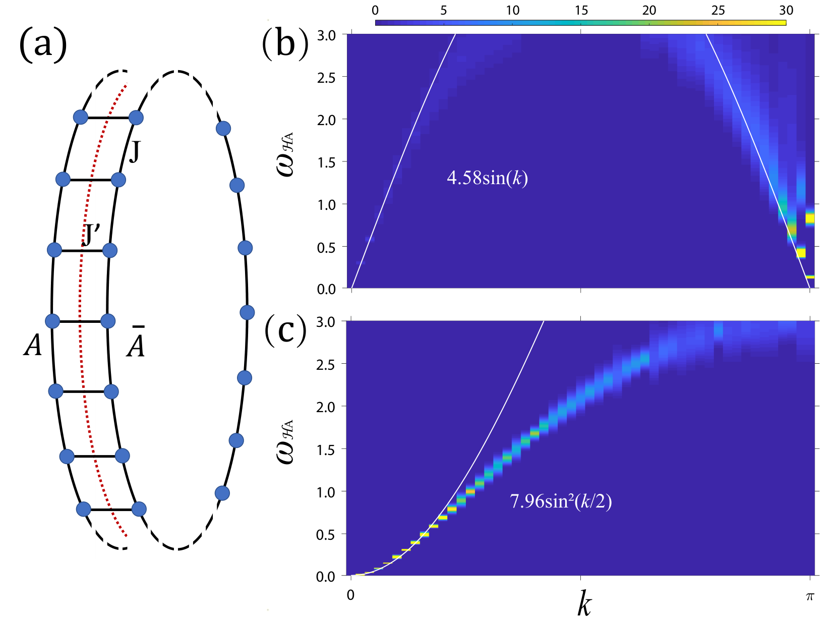
An earlier replica-QMC approach reconstructed the leading, particle-number-resolved levels of the entanglement spectrum from measured moments of the RDM, with the eigenvalues obtained by solving a polynomial root-finding problem 36.
Going beyond the reconstruction of a few leading eigenvalues, Ref. 209 developed a multi-replica QMC approach for bosonic and spin systems that extracts the low-lying entanglement spectral function through stochastic analytic continuation of imaginary-time correlation functions 165. This approach provides spectral information indirectly, through the reconstruction of a dynamical response associated with the entanglement Hamiltonian. The key idea is to simulate , where the power can be treated as an effective inverse temperature for the entanglement Hamiltonian , so that the dynamics of is contained in the effective imaginary-time correlators. As Fig. 18 shows, a super long entanglement cut can be calculated but the result is limited to the spectral function of the entanglement Hamiltonian instead of a full spectrum. The advantage of this method is that large systems can be simulated, meanwhile, the disadvantage is the rough precision due to the analytical continuation and integer imaginary-time. A method based on a similar idea has also been proposed for fermionic systems 10.
By contrast, Ref. 124 introduced the RDM sampling approach discussed in this section. The method directly reconstructs , whose diagonalization resolves the fine, individual levels of the entanglement spectrum.
A representative application is the Néel-ordered phase of the D square-lattice antiferromagnetic Heisenberg model. More generally, for a finite D quantum system whose thermodynamic limit spontaneously breaks the continuous symmetry, the low-lying physical energy spectrum contains an Anderson tower of states (TOS) 9; 16, with
| (228) |
where labels the total angular-momentum quantum number and is the transverse susceptibility in the thermodynamic limit. For the D Heisenberg model, for which and , Eq. (228) reduces to
| (229) |
An analogous TOS structure is expected to appear in the low-lying entanglement spectrum of ground states exhibiting SSB of a continuous symmetry 2; 96.
As shown in Fig. 19, the directly reconstructed entanglement spectrum exhibits this TOS organization for both a ring-shaped subsystem and a square-block subsystem. This example illustrates how direct sampling of the RDM resolves the individual low-lying levels and their multiplet structure, which would not be accessible from a scalar entanglement entropy alone.
A further application of this approach was demonstrated in Ref. 125, where the tower-of-states structure in the entanglement spectrum of a small subsystem was used to identify the underlying continuous symmetry of a quantum critical point. In particular, this provides a direct probe of emergent continuous symmetries without requiring prior knowledge of the corresponding order parameters or low-energy effective field theory.
V.6.2 Few-site correlation functions, multipartite entanglement, and long-range quantum magic
Once the RDM of a subsystem has been reconstructed, it can be used to evaluate any equal-time observable supported within that subsystem. In particular, if consists of two possibly separated groups of sites, then for arbitrary operators and supported on the respective regions,
| (230) |
Thus, a single reconstructed RDM contains all equal-time correlation functions between operators supported on and , rather than only a predetermined set of conventional observables, as exploited in Ref. 34. More generally, this approach provides a systematic way to measure off-diagonal operators in QMC, rather than relying on the extraction of Green’s functions within a worm-update scheme 49.
Direct access to few-site RDMs also enables the study of multipartite entanglement. In Ref. 195, they used reconstructed two- and three-site density matrices to investigate bipartite negativity and genuine tripartite entanglement. This program was subsequently extended to RDMs containing up to four sites, allowing three- and four-party genuine multipartite entanglement to be examined across the quantum Ising models in one, two, and three spatial dimensions 122.
Beyond entanglement, the same framework provides access to nonlinear mixed-state measures of quantum magic or nonstabilizerness. In Ref. 181, RDMs of spatially separated partitions were combined with numerical computations of the robustness of magic 81 to quantify the long-range quantum magic. At the quantum critical point of the 1D quantum Ising model, this quantity exhibits an algebraic decay with the separation between the partitions, revealing long-range magic correlations.
V.6.3 Nonequal-Time Observables and the Rényi-1 Correlator for SWSSB in the RDM-QMC
As discussed in Sec. II.2.4, the reduced-density-matrix sampling framework can be generalized to operator-inserted RDMs, as introduced in Sec. II.8. The key idea is to insert the measured operator at a specific imaginary-time slice to construct a generalized RDMs, from which imaginary-time observables can be extracted. This generalized sampling scheme was implemented in Ref. 200, providing QMC access to both equal- and nonequal-imaginary-time observables, including off-diagonal correlation functions and, through analytic continuation 165, dynamical spectral functions.
An important application in many-body quantum information is the Rényi-1, or Wightman, correlator 202; 115 to Gibbs states,
| (231) |
where is a symmetry-neutral bilocal operator constructed from local operators carrying nontrivial symmetry charge, for example .
FIG. 20. Rényi-1 correlator in the D XXZ model. (a) as a function of the anisotropy for square lattices with . In the ground-state limit (), maintains a finite value throughout the parameter space. (b) Finite-size scaling of at the pure XY point () across various temperatures. The correlator exhibits a distinct plateau in the large- regime. (c) The dashed vertical line marks the Berezinskii-Kosterlitz-Thouless transition temperature . The signal evolves smoothly across , and no behavioral changes are observed on either side of the phase transition. All data were computed using the generalized RDM framework. Figure from Ref. 200.
For a Gibbs state, , Eq. (231) can be written as an nonequal-imaginary-time correlation function,
| (232) |
It can therefore be evaluated through an operator insertion at , without explicitly constructing . In an appropriate fixed symmetry-charge sector, long-range order in can diagnose strong-to-weak spontaneous symmetry breaking even when the corresponding conventional two-point correlation function remains short-ranged. The authors took the 2D quantum XXZ model as an example to demonstrate the SWSSB, as shown in Fig. V.6.3.
VI Summary
In this review, we have presented a unified perspective on how, over nearly two decades, QMC methods have evolved into a general framework for studying many-body quantum information beyond conventional observables. The organizing principle, developed in Sec. II, is that the scope of QMC is determined less by the Hamiltonian itself than by the class of density matrices—and generalized density-matrix-like objects—that admit sign-problem-free configuration-space representations. From this perspective, conventional Gibbs-state QMC and ground-state projector QMC emerge as two standard representatives of a much broader family of constructions, including reduced density matrices, replicated states, partially transposed replicated states, operator-inserted density matrices, and states evolving under quantum channels. These seemingly different constructions can be described within a common language of boundary connectivity: traces, partial traces, cyclic replica gluings, and channel-induced constraints correspond to different ways of identifying, closing, or constraining the open transfer-direction boundary indices of a density matrix.
This framework further clarifies how an appropriate choice of basis can transform an otherwise difficult nonlinear quantity into an ordinary QMC observable. In the valence-bond basis and the Bell basis discussed in Sec. III, SWAP operators admit direct estimators, allowing the Rényi-2 entropy to be measured without evaluating partition-function ratios. In the Bell basis, moreover, the full Pauli spectrum can be sampled directly, providing access to the characteristic distribution used in stabilizer-entropy diagnostics of quantum magic.
The second pillar of the modern formulation, reviewed in Sec. IV, is the toolkit for evaluating generalized partition-function ratios, to which Rényi-type quantities can ultimately be reduced. This toolkit includes extended ensembles with sector-switch updates, reweighting–annealing schemes, thermodynamic integration, derivative estimators, continuous extended ensembles, and nonequilibrium work estimators based on Jarzynski’s equality. Together with the incremental trick, which avoids the direct estimation of exponentially small ratios, these techniques can recast certain nonlinear observables into more stable sampling problems. In favorable cases, this can substantially reduce the computational cost and make QMC calculations feasible for system sizes beyond those accessible by direct estimators.
The applications reviewed in Sec. V demonstrate the broad reach of these developments. QMC now provides high-precision access to entanglement entropies and their universal subleading contributions, including Goldstone-mode logarithmic corrections, central charges, topological entanglement entropy, and entanglement derivatives with characteristic critical scaling. It also enables the study of mixed-state entanglement through Rényi negativities, with quantitative tests of CFT predictions and finite-temperature critical behavior; many-body magic through stabilizer entropies and their connections to BCFT; composite information-theoretic quantities such as mutual information; and SWSSB in decohered quantum states. More recently, direct sampling of reduced density matrices has opened access to the entanglement spectrum and its tower-of-states structure and emergent symmetries, as well as multipartite entanglement, long-range mixed-state magic, and the Rényi-1 correlator. Taken together, these developments substantiate a density-matrix-centered formulation of QMC in which statistical sampling and quantum-information structure are treated on equal footing.
Finally, the developments reviewed here point to a deeper convergence among classical simulation, quantum information, and many-body physics. Concepts imported from quantum information—Bell sampling and the stabilizer formalism in particular—have become native tools in QMC, while QMC in turn provides a classical laboratory for information-theoretic diagnostics at system sizes far beyond current quantum devices. We hope that the unified viewpoint presented in this review will serve as a useful guide and entry point for readers from the QMC, quantum-information, many-body, and condensed-matter communities, and will stimulate further developments at their interfaces.
Acknowledgements
We are grateful to Zhe Wang, Yanzhang Zhu, and Yan Liu for carefully reading the manuscript and providing valuable comments and suggestions. We also thank our collaborators Zhiyan Wang, Zenan Liu, Xu Tian, Poetri Sonya Tarabunga, Jiarui Zhao, Gaopei Pan, and Weilun Jiang for their contributions to the related algorithmic works reviewed here and for many insightful discussions throughout these projects. We further thank Zi Yang Meng, Yan-Cheng Wang, Sylvain Capponi, Fabien Alet, Wenan Guo and Youjin Deng for helpful discussions on related algorithms.
References
- Improved simulation of stabilizer circuits. Physical Review A 70 (5). External Links: ISSN 1094-1622, Link, Document Cited by: §V.3.1.
- Entanglement spectrum of the two-dimensional bose-hubbard model. Phys. Rev. Lett. 110, pp. 260403. External Links: Document, Link Cited by: §V.6.1.
- Entanglement negativity and conformal field theory: a monte carlo study. Journal of Statistical Mechanics: Theory and Experiment 2013 (05), pp. P05013. External Links: Document, Link Cited by: §V.2.2.
- Symmetries and conserved quantities in lindblad master equations. Phys. Rev. A 89, pp. 022118. External Links: Document, Link Cited by: §II.9.2.
- Valence bond entanglement entropy. Phys. Rev. Lett. 99, pp. 117204. External Links: Document, Link Cited by: §II.4.1, §III.
- Generalized directed loop method for quantum monte carlo simulations. Phys. Rev. E 71, pp. 036706. External Links: Document, Link Cited by: §II.3.
- Trace index and spectral flow in the entanglement spectrum of topological insulators. Phys. Rev. B 84, pp. 195103. External Links: Document, Link Cited by: §V.6.1.
- Entanglement in many-body systems. Rev. Mod. Phys. 80, pp. 517–576. External Links: Document, Link Cited by: §I, §I, §V.1.1.
- An approximate quantum theory of the antiferromagnetic ground state. Phys. Rev. 86, pp. 694–701. External Links: Document, Link Cited by: §V.6.1.
- Entanglement spectra of interacting fermions in quantum monte carlo simulations. Phys. Rev. B 89, pp. 125121. External Links: Document, Link Cited by: §V.6.1.
- Post-measurement quantum monte carlo. Phys. Rev. B 112, pp. 184417. External Links: Document, Link Cited by: §II.9.
- Some formal results for the valence bond basis. Nuclear Physics B 750 (3), pp. 142–178. External Links: Document, cond-mat/0605103 Cited by: §III.1.1.
- Simulations of discrete quantum systems in continuous euclidean time. Phys. Rev. Lett. 77, pp. 5130–5133. External Links: Document, Link Cited by: §II.3.
- Universality of magic in local quantum field theory. External Links: 2607.16403, Link Cited by: §V.3.2.
- Efficient estimation of free energy differences from monte carlo data. Journal of Computational Physics 22 (2), pp. 245–268. External Links: ISSN 0021-9991, Document, Link Cited by: §III.1.3, §IV.2.
- Signature of néel order in exact spectra of quantum antiferromagnets on finite lattices. Phys. Rev. Lett. 69, pp. 2590–2593. External Links: Document, Link Cited by: §V.6.1.
- Quantum simulations with ultracold quantum gases. Nature Physics 8 (4), pp. 267–276. External Links: ISSN 1745-2481, Document, Link Cited by: §I.
- Kagome model for a quantum spin liquid. Phys. Rev. B 101, pp. 020402(R). External Links: Document, Link Cited by: §V.4.
- Conformal invariance, the central charge, and universal finite-size amplitudes at criticality. Phys. Rev. Lett. 56, pp. 742–745. External Links: Document, Link Cited by: §V.2.2.
- Merlin-arthur games and stoquastic complexity. External Links: quant-ph/0611021, Link Cited by: §I.
- The complexity of stoquastic local hamiltonian problems. Quantum Info. Comput. 8 (5), pp. 361–385. External Links: ISSN 1533-7146 Cited by: §I.
- Universal quantum computation with ideal clifford gates and noisy ancillas. Phys. Rev. A 71, pp. 022316. External Links: Document, Link Cited by: §V.3.1.
- Probing rényi entanglement entropy via randomized measurements. Science 364 (6437), pp. 260–263. External Links: Document, Link, https://www.science.org/doi/pdf/10.1126/science.aau4963 Cited by: §I.
- A note on symmetry reductions of the lindblad equation: transport in constrained open spin chains. New Journal of Physics 14 (7), pp. 073007. External Links: Document, Link Cited by: §II.9.2.
- Entanglement negativity in quantum field theory. Phys. Rev. Lett. 109, pp. 130502. External Links: Document, Link Cited by: §II.7.
- Entanglement negativity in extended systems: a field theoretical approach. Journal of Statistical Mechanics: Theory and Experiment 2013, pp. P02008. External Links: Document Cited by: §II.7, §V.2.2, §V.2.2.
- Entanglement entropy and quantum field theory. Journal of Statistical Mechanics: Theory and Experiment 2004 (06), pp. P06002. External Links: Document, Link Cited by: §II.6.1, §V.1.1.
- Entanglement entropy and conformal field theory. Journal of Physics A: Mathematical and Theoretical 42 (50), pp. 504005. External Links: Document, Link Cited by: §I, §V.1.1, §V.1.1, §V.1.2.
- Entanglement spectrum in one-dimensional systems. Phys. Rev. A 78, pp. 032329. External Links: Document, Link Cited by: §V.6.1.
- On geometric entropy. Physics Letters B 333 (1), pp. 55–61. External Links: ISSN 0370-2693, Document, Link Cited by: §II.6.1.
- Path integrals in the theory of condensed helium. Rev. Mod. Phys. 67, pp. 279–355. External Links: Document, Link Cited by: §II.2.1.
- Bulk-edge correspondence in entanglement spectra. Phys. Rev. B 84, pp. 205136. External Links: Document, Link Cited by: §V.6.1.
- Theory of trotter error with commutator scaling. Phys. Rev. X 11, pp. 011020. External Links: Document, Link Cited by: §II.3.1.
- Detecting the largest correlations for many-body systems using the correlation density matrix: a quantum monte carlo approach. Phys. Rev. B 113, pp. 035122. External Links: Document, Link Cited by: §II.2.4, §II.5, §V.6.2.
- Entanglement negativity via the replica trick: a quantum monte carlo approach. Phys. Rev. B 90, pp. 064401. External Links: Document, Link Cited by: §V.2.1.
- Entanglement spectroscopy using quantum monte carlo. Physical Review B 89 (19), pp. 195147. External Links: Document, 1305.6536 Cited by: §V.6.1.
- Matrix product states and projected entangled pair states: concepts, symmetries, theorems. Rev. Mod. Phys. 93, pp. 045003. External Links: Document, Link Cited by: §I.
- Entanglement spectrum and boundary theories with projected entangled-pair states. Phys. Rev. B 83, pp. 245134. External Links: Document, Link Cited by: §V.6.1.
- Extracting universal corner entanglement entropy during the quantum monte carlo simulation. Phys. Rev. B 110, pp. 235111. External Links: Document, Link Cited by: §V.1.2.
- Residual entropy from the temperature incremental monte carlo method. Phys. Rev. B 111, pp. L081108. External Links: Document, Link Cited by: §IV.3.
- Genuine quantum correlations in quantum many-body systems: a review of recent progress. Reports on Progress in Physics 81 (7), pp. 074002. External Links: Document, Link Cited by: §I.
- ’T hooft loop in su(2) yang-mills theory. Phys. Rev. Lett. 86, pp. 1438–1441. External Links: Document, Link Cited by: §III.1.3, §IV.3.
- Diagnosing quantum phase transition order and deconfined criticality via entanglement entropy. Phys. Rev. Lett. 133, pp. 100402. External Links: Document, Link Cited by: §V.1.2.
- Strong-to-weak spontaneous symmetry breaking in a d transverse-field ising model under decoherence. External Links: 2603.24342, Link Cited by: Figure 7, Figure 7, §II.9.2, §II.9.2, §II.9.2, §II.9, Figure 17, Figure 17, §V.5.
- Mixed-state measurement-induced phase transitions in imaginary-time dynamics. External Links: 2511.04402, Link Cited by: §II.9.1, §II.9.1, §II.9.
- Reweight-annealing method for evaluating the partition function via quantum monte carlo calculations. Phys. Rev. B 110, pp. 165152. External Links: Document, Link Cited by: §IV.1, §IV.3, §IV.3, §V.1.2.
- Tracking the variation of entanglement rényi negativity: a quantum monte carlo study. Phys. Rev. B 111, pp. L241108. External Links: Document, Link Cited by: §IV.3, §IV.3, Figure 13, Figure 13, §V.2.2, §V.2.2.
- Evaluating many-body stabilizer rényi entropy by sampling reduced pauli strings: singularities, volume law, and nonlocal magic. PRX Quantum 6, pp. 030328. External Links: Document, Link Cited by: §IV.5, §IV.5, Figure 15, Figure 15, Figure 16, Figure 16, §V.3.1, §V.3.2, §V.3.3, §V.4.
- Accessing the dynamics of large many-particle systems using the stochastic series expansion. Phys. Rev. E 64, pp. 066701. External Links: Document, Link Cited by: §V.6.2.
- Real-space entanglement spectrum of quantum hall systems. Phys. Rev. B 85, pp. 115321. External Links: Document, Link Cited by: §V.6.1.
- Rényi entanglement entropy of critical spin chains. Phys. Rev. B 92, pp. 054411. External Links: Document, Link Cited by: §V.1.2.
- Entanglement entropy and deconfined criticality: emergent so(5) symmetry and proper lattice bipartition. Phys. Rev. Lett. 133, pp. 166702. External Links: Document, Link Cited by: §IV.6, §V.1.2.
- Entanglement entropy from nonequilibrium work. Phys. Rev. Lett. 124, pp. 110602. External Links: Document, Link Cited by: §IV.6, §IV.6, §IV.7, §IV.7, §IV.7, §V.1.2, §V.1.2.
- Colloquium: area laws for the entanglement entropy. Rev. Mod. Phys. 82, pp. 277–306. External Links: Document, Link Cited by: §I, §I, §V.1.1.
- The loop algorithm. Advances in Physics 52 (1), pp. 1–66. External Links: Document, Link, https://doi.org/10.1080/0001873021000049195 Cited by: §II.3.
- Two-point stabilizer rényi entropy: a computable magic proxy of interacting fermions. External Links: 2601.13314, Link Cited by: §V.4.
- Fermionic partial transpose in the overlap matrix framework for entanglement negativity. Phys. Rev. B 112, pp. 075154. External Links: Document, Link Cited by: §V.2.2.
- New monte carlo technique for studying phase transitions. Phys. Rev. Lett. 61, pp. 2635–2638. External Links: Document, Link Cited by: §IV.3.
- Entanglement spectrum of topological insulators and superconductors. Phys. Rev. Lett. 104, pp. 130502. External Links: Document, Link Cited by: §V.6.1.
- Topological entanglement rényi entropy and reduced density matrix structure. Phys. Rev. Lett. 103, pp. 261601. External Links: Document, Link Cited by: §V.1.2.
- Chapter 7 - free energy calculations. In Understanding Molecular Simulation (Second Edition), D. Frenkel and B. Smit (Eds.), pp. 167–200. External Links: ISBN 978-0-12-267351-1, Document, Link Cited by: §IV.1.
- Probing quantum correlations in many-body systems: a review of scalable methods. Reports on Progress in Physics 86 (11), pp. 114001. External Links: Document, Link Cited by: §I.
- Simulating normalizing constants: from importance sampling to bridge sampling to path sampling. Statistical Science 13 (2), pp. 163 – 185. External Links: Document, Link Cited by: §IV.1.
- Quantum simulation. Rev. Mod. Phys. 86, pp. 153–185. External Links: Document, Link Cited by: §I.
- Probing chaos by magic monotones. Phys. Rev. D 106, pp. 126009. External Links: Document, Link Cited by: §V.3.1.
- Stabilizer codes and quantum error correction. External Links: quant-ph/9705052, Link Cited by: §V.3.1.
- Schur–weyl duality for the clifford group with applications: property testing, a robust hudson theorem, and de finetti representations. Communications in Mathematical Physics 385 (3), pp. 1325–1393. External Links: ISSN 1432-0916, Document, Link Cited by: §III.2.2.
- Generalized li-haldane correspondence in critical free-fermion systems. Phys. Rev. Res. 8, pp. 023203. External Links: Document, Link Cited by: §V.6.1.
- The monte carlo method in quantum statistical mechanics. Mathematical Proceedings of the Cambridge Philosophical Society 58, pp. 594 – 598. External Links: Link Cited by: §II.3.
- Measuring renyi entanglement entropy in quantum monte carlo simulations. Phys. Rev. Lett. 104, pp. 157201. External Links: Document, Link Cited by: §II.4.1, §III.1.2, §III.1.3, §III.1.3, §III.
- Efficient quantum algorithms for stabilizer entropies. Physical Review Letters 132 (24), pp. 240602. External Links: Document Cited by: §III.2.2.
- Quantifying nonstabilizerness of matrix product states. Phys. Rev. B 107, pp. 035148. External Links: Document, Link Cited by: §V.3.1.
- Stabilizer entropies and nonstabilizerness monotones. Quantum 7, pp. 1092. External Links: Document, Link, ISSN 2521-327X Cited by: §V.3.1, §V.3.1.
- Entanglement entropy scaling in the bilayer heisenberg spin system. Phys. Rev. B 89, pp. 245120. External Links: Document, Link Cited by: §V.1.3.
- Sign problem in monte carlo simulations of frustrated quantum spin systems. Physical Review B 62, pp. 1102–1113. External Links: Document Cited by: §I, §II.2.2.
- Geometric and renormalized entropy in conformal field theory. Nuclear Physics B 424 (3), pp. 443–467. External Links: ISSN 0550-3213, Document, Link Cited by: §II.6.1.
- Separability of mixed states: necessary and sufficient conditions. Physics Letters A 223 (1), pp. 1–8. External Links: ISSN 0375-9601, Document, Link Cited by: §II.7, §V.2.1.
- Quantum entanglement. Rev. Mod. Phys. 81, pp. 865–942. External Links: Document, Link Cited by: §I, §V.1.1.
- Stabilizer rényi entropy encodes fusion rules of topological defects and boundaries. Phys. Rev. Lett. 136, pp. 080402. External Links: Document, Link Cited by: §V.3.1, §V.3.2.
- Stabilizer rényi entropy and conformal field theory. Phys. Rev. X 16, pp. 011037. External Links: Document, Link Cited by: §V.3.1, §V.3.2, §V.3.2.
- Application of a resource theory for magic states to fault-tolerant quantum computing. Phys. Rev. Lett. 118, pp. 090501. External Links: Document, Link Cited by: §V.6.2.
- Contextuality supplies the ‘magic’ for quantum computation. Nature 510 (7505), pp. 351–355. External Links: ISSN 1476-4687, Document, Link Cited by: §V.3.1.
- Quantum monte carlo calculation of entanglement rényi entropies for generic quantum systems. Phys. Rev. B 86, pp. 235116. External Links: Document, Link Cited by: §IV.2, §IV.2, §IV.2.
- Wang-landau method for calculating rényi entropies in finite-temperature quantum monte carlo simulations. Phys. Rev. E 87, pp. 013306. External Links: Document, Link Cited by: §IV.1.
- Wang-landau method for calculating rényi entropies in finite-temperature quantum monte carlo simulations. Physical Review E 87 (1). External Links: ISSN 1550-2376, Link, Document Cited by: §V.4.
- Topological entanglement entropy of a bose–hubbard spin liquid. Nature Physics 7 (10), pp. 772–775. External Links: ISSN 1745-2481, Document, Link Cited by: §V.1.2, §V.4.
- Nonequilibrium equality for free energy differences. Phys. Rev. Lett. 78, pp. 2690–2693. External Links: Document, Link Cited by: §IV.7, §IV.7, §IV.7.
- Valence bond and von neumann entanglement entropy in heisenberg ladders. Phys. Rev. Lett. 103, pp. 117203. External Links: Document, Link Cited by: §II.4.1, §III.
- Anomalies in the entanglement properties of the square-lattice heisenberg model. Phys. Rev. B 84, pp. 165134. External Links: Document, Link Cited by: §V.4.
- Contact Electron-Spin Coupling of Nuclear Magnetic Moments. J. Chem. Phys. 30 (1), pp. 11–15. External Links: Document Cited by: §IV.3.
- Quantum thermalization through entanglement in an isolated many-body system. Science 353 (6301), pp. 794–800. External Links: Document, Link, https://www.science.org/doi/pdf/10.1126/science.aaf6725 Cited by: §I.
- Bridging lattice-scale physics and continuum field theory with quantum monte carlo simulations. Annual Review of Condensed Matter Physics 4 (Volume 4, 2013), pp. 179–215. External Links: Document, Link, ISSN 1947-5462 Cited by: §II.4.1, §III.
- Recent developments of world-line monte carlo methods. Journal of the Physical Society of Japan 73, pp. 1379–1414. Cited by: §II.3.
- Optimization by simulated annealing. Science 220 (4598), pp. 671–680. External Links: Document Cited by: §IV.3.
- Topological entanglement entropy. Phys. Rev. Lett. 96, pp. 110404. External Links: Document, Link Cited by: §V.1.2.
- Entanglement spectroscopy of su(2)-broken phases in two dimensions. Phys. Rev. B 88, pp. 144426. External Links: Document, Link Cited by: §V.6.1.
- Detecting goldstone modes with entanglement entropy. Phys. Rev. B 92, pp. 115146. External Links: Document, Link Cited by: §V.1.2.
- Pseudocriticality in antiferromagnetic spin chains. Phys. Rev. Lett. 136, pp. 076701. External Links: Document, Link Cited by: §V.1.2.
- Quantum entanglement in condensed matter systems. Physics Reports 646, pp. 1–59. Note: Quantum entanglement in condensed matter systems External Links: ISSN 0370-1573, Document, Link Cited by: §I, §I, §V.1.1.
- Nonstabilizerness via perfect pauli sampling of matrix product states. Phys. Rev. Lett. 131, pp. 180401. External Links: Document, Link Cited by: §V.3.1.
- A short review on entanglement in quantum spin systems. Journal of Physics A: Mathematical and Theoretical 42 (50), pp. 504002. External Links: Document, Link Cited by: §I, §V.1.1.
- Disentangling entanglement spectra of fractional quantum hall states on torus geometries. Phys. Rev. Lett. 104, pp. 156404. External Links: Document, Link Cited by: §V.6.1.
- Quantum criticality under decoherence or weak measurement. PRX Quantum 4, pp. 030317. External Links: Document, Link Cited by: §II.9.2, §V.5.
- Stabilizer entropies are monotones for magic-state resource theory. Phys. Rev. A 110, pp. L040403. External Links: Document, Link Cited by: §V.3.1, §V.3.1.
- Stabilizer rényi entropy. Phys. Rev. Lett. 128, pp. 050402. External Links: Document, Link Cited by: §III.2.2, §V.3.1, §V.3.1, §V.3.1, §V.3.1.
- Quantum Chaos is Quantum. Quantum 5, pp. 453. External Links: Document, Link, ISSN 2521-327X Cited by: §V.3.1.
- Strong-to-weak spontaneous symmetry breaking in mixed quantum states. PRX Quantum 6, pp. 010344. External Links: Document, Link Cited by: §II.9.2, §V.5.
- Detecting topological order in a ground state wave function. Phys. Rev. Lett. 96, pp. 110405. External Links: Document, Link Cited by: §V.1.2.
- Entanglement spectrum as a generalization of entanglement entropy: identification of topological order in non-abelian fractional quantum hall effect states. Phys. Rev. Lett. 101, pp. 010504. External Links: Document, Link Cited by: §V.6.1, §V.6.1.
- Sign-problem-free fermionic quantum monte carlo: developments and applications. Annual Review of Condensed Matter Physics 10, pp. 337–356. External Links: Document Cited by: §I, §II.2.2.
- Existence of néel order at t=0 in the spin-1/2 antiferromagnetic heisenberg model on a square lattice. Phys. Rev. B 42, pp. 6555–6560. External Links: Document, Link Cited by: §II.4.1, §III.
- Symmetry breaking and error correction in open quantum systems. Phys. Rev. Lett. 125, pp. 240405. External Links: Document, Link Cited by: §II.9.2.
- Entanglement rényi negativity across the finite-temperature transition in the universality class. Phys. Rev. B 113, pp. 245145. External Links: Document, Link Cited by: §V.2.2, §V.2.3.
- Nonequilibrium quantum monte carlo algorithm for stabilizer rényi entropy in spin systems. Phys. Rev. B 111, pp. 085144. External Links: Document, Link Cited by: §V.3.1, §V.4.
- Diagnosing strong-to-weak symmetry breaking via wightman correlators. Communications Physics 8 (1), pp. 274. External Links: ISSN 2399-3650, Document, Link Cited by: §V.6.3.
- Many-body quantum magic. PRX Quantum 3, pp. 020333. External Links: Document, Link Cited by: §I, §V.3.1.
- Antiferromagnetic to valence-bond-solid transitions in two-dimensional heisenberg models with multispin interactions. Phys. Rev. B 80, pp. 180414(R). External Links: Document, Link Cited by: §V.1.2.
- Singularity in entanglement negativity across finite-temperature phase transitions. Phys. Rev. B 99, pp. 075157. External Links: Document, Link Cited by: §V.2.3.
- Structure of quantum entanglement at a finite temperature critical point. Phys. Rev. Res. 2, pp. 043345. External Links: Document, Link Cited by: §V.2.3.
- Detecting topological order at finite temperature using entanglement negativity. Phys. Rev. Lett. 125, pp. 116801. External Links: Document, Link Cited by: §V.2.2.
- Universal logarithmic corrections to entanglement entropies in two dimensions with spontaneously broken continuous symmetries. Physical Review B 91, pp. 155145. External Links: Document Cited by: §V.1.2.
- Multiparty entanglement microscopy of quantum ising models in one, two, and three dimensions. Phys. Rev. B 111, pp. 245108. External Links: Document, Link Cited by: §II.2.4, §V.6.2.
- Defining a universal sign to strictly probe a phase transition. Phys. Rev. B 110, pp. 125141. External Links: Document, Link Cited by: §IV.3.
- Sampling reduced density matrix to extract fine levels of entanglement spectrum and restore entanglement hamiltonian. Nature Communications 16 (1), pp. 2880. External Links: ISSN 2041-1723, Document, Link Cited by: §II.2.1, §II.2.4, §II.5, Figure 19, Figure 19, §V.6.1.
- Detecting the emergent continuous symmetry of criticality via a subsystem’s entanglement spectrum. Phys. Rev. Lett. 136, pp. 046401. External Links: Document, Link Cited by: §II.2.4, §V.6.1.
- Finite-size scaling of mutual information in monte carlo simulations: application to the spin- model. Phys. Rev. B 82, pp. 100409(R). External Links: Document, Link Cited by: §V.4.
- Finite-size scaling of mutual information in monte carlo simulations: application to the spin- model. Phys. Rev. B 82, pp. 100409(R). External Links: Document, Link Cited by: §IV.4, §IV.4.
- Stochastic series expansion algorithm for the model with four-site ring exchange. Phys. Rev. E 72, pp. 026702. External Links: Document, Link Cited by: §II.3.
- Stochastic series expansion quantum monte carlo. In Strongly Correlated Systems: Numerical Methods, A. Avella and F. Mancini (Eds.), pp. 185–206. External Links: ISBN 978-3-642-35106-8, Document, Link Cited by: §II.3, §II.4.1, §III.
- Measuring von neumann entanglement entropies without wave functions. New Journal of Physics 22 (1), pp. 013044. External Links: Document, Link Cited by: §IV.1, §V.1.1.
- Entanglement entropy in the model. Phys. Rev. B 80, pp. 115122. External Links: Document, Link Cited by: §V.1.2, §V.1.3.
- Entanglement entropy of systems with spontaneously broken continuous symmetry. External Links: 1112.5166, Link Cited by: §V.1.2.
- Path integral monte carlo calculation of the momentum distribution of the homogeneous electron gas at finite temperature. External Links: cond-mat/0310401, Link Cited by: §II.2.1.
- Detecting entanglement from few partial transpose moments and their decay via weight enumerators. External Links: 2604.12576 Cited by: §V.2.1.
- Learning stabilizer states by bell sampling. External Links: 1707.04012, Link Cited by: §III.2.2, §III.2.2.
- Probabilistic inference using markov chain monte carlo methods. . Cited by: §IV.1.
- Symmetry-resolved entanglement detection using partial transpose moments. npj Quantum Information 7, pp. 152. External Links: Document Cited by: §V.2.1.
- Quantum computation and quantum information. 10th Anniversary edition, Cambridge University Press, Cambridge. External Links: ISBN 978-1-107-00217-3, Document Cited by: §II.9.
- Magic-state resource theory for the ground state of the transverse-field ising model. Phys. Rev. A 106, pp. 042426. External Links: Document, Link Cited by: §V.3.1.
- Thermodynamic limit of density matrix renormalization. Phys. Rev. Lett. 75, pp. 3537–3540. External Links: Document, Link Cited by: §I.
- The sign problem in quantum monte carlo simulations. In Encyclopedia of Condensed Matter Physics (Second Edition), T. Chakraborty (Ed.), pp. 879–893. External Links: ISBN 978-0-323-91408-6, Document, Link Cited by: §I, §II.2.2.
- The rényi entanglement entropy of a general quantum dimer model at the rk point: a highly efficient algorithm. Journal of Physics: Condensed Matter 26 (3), pp. 035601. External Links: Document, Link Cited by: §V.1.2.
- Separability criterion for density matrices. Phys. Rev. Lett. 77, pp. 1413–1415. External Links: Document, Link Cited by: §II.7, §V.2.1.
- Logarithmic negativity: a full entanglement monotone that is not convex. Phys. Rev. Lett. 95, pp. 090503. External Links: Document, Link Cited by: §V.2.1.
- Entanglement spectra of quantum heisenberg ladders. Phys. Rev. Lett. 105, pp. 077202. External Links: Document, Link Cited by: §V.6.1.
- Symmetry protection of topological phases in one-dimensional quantum spin systems. Phys. Rev. B 85, pp. 075125. External Links: Document, Link Cited by: §V.6.1.
- Entanglement spectrum of a topological phase in one dimension. Phys. Rev. B 81, pp. 064439. External Links: Document, Link Cited by: §V.6.1, §V.6.1.
- Entanglement spectrum of a disordered topological chern insulator. Phys. Rev. Lett. 105, pp. 115501. External Links: Document, Link Cited by: §V.6.1.
- Exact, complete, and universal continuous-time worldline monte carlo approach to the statistics of discrete quantum systems. Journal of Experimental and Theoretical Physics 87 (2), pp. 310–321. External Links: ISSN 1090-6509, Document, Link Cited by: §II.3.
- General relationship between the entanglement spectrum and the edge state spectrum of topological quantum states. Phys. Rev. Lett. 108, pp. 196402. External Links: Document, Link Cited by: §V.6.1.
- Quantum nonlocal nonstabilizerness. Phys. Rev. A 111, pp. 052443. External Links: Document, Link Cited by: §V.3.1.
- A generalization of handscomb’s quantum monte carlo scheme-application to the 1d hubbard model. Journal of Physics A: Mathematical and General 25 (13), pp. 3667. External Links: Document, Link Cited by: §II.3.
- Monte carlo simulations of quantum spin systems in the valence bond basis. External Links: 0704.1469, Link Cited by: §II.4.1, §III.
- Loop updates for variational and projector quantum monte carlo simulations in the valence-bond basis. Phys. Rev. B 82, pp. 024407. External Links: Document, Link Cited by: §II.4.1, §III.
- Stochastic series expansion method with operator-loop update. Phys. Rev. B 59, pp. R14157(R)–R14160(R). External Links: Document, Link Cited by: §II.3.
- Stochastic series expansion method for quantum ising models with arbitrary interactions. Phys. Rev. E 68, pp. 056701. External Links: Document, Link Cited by: §II.3.
- Ground state projection of quantum spin systems in the valence-bond basis. Phys. Rev. Lett. 95, pp. 207203. External Links: Document, Link Cited by: §II.4.1, §III.1.1, §III.1.1, §III.
- Evidence for deconfined quantum criticality in a two-dimensional heisenberg model with four-spin interactions. Phys. Rev. Lett. 98, pp. 227202. External Links: Document, Link Cited by: §V.1.2.
- Continuous quantum phase transition between an antiferromagnet and a valence-bond solid in two dimensions: evidence for logarithmic corrections to scaling. Phys. Rev. Lett. 104, pp. 177201. External Links: Document, Link Cited by: §V.1.2.
- Stochastic series expansion methods. External Links: 1909.10591, Link Cited by: §II.3.
- Characterization of an operational quantum resource in a critical many-body system. New Journal of Physics 22 (8), pp. 083077. External Links: Document, Link Cited by: §V.3.1.
- The density-matrix renormalization group. Rev. Mod. Phys. 77, pp. 259–315. External Links: Document, Link Cited by: §I.
- Entanglement entropy at generalized rokhsar-kivelson points of quantum dimer models. Phys. Rev. B 87, pp. 125105. External Links: Document, Link Cited by: §V.1.2.
- Example of a first-order néel to valence-bond-solid transition in two dimensions. Phys. Rev. B 82, pp. 174428. External Links: Document, Link Cited by: §V.1.2.
- Progress on stochastic analytic continuation of quantum monte carlo data. Physics Reports 1003, pp. 1–88. Note: Progress on stochastic analytic continuation of quantum Monte Carlo data External Links: ISSN 0370-1573, Document, Link Cited by: §V.6.1, §V.6.3.
- Benchmarking highly entangled states on a 60-atom analogue quantum simulator. Nature 628 (8006), pp. 71–77. External Links: ISSN 1476-4687, Document, Link Cited by: §I.
- Finite-temperature critical behavior of mutual information. Phys. Rev. Lett. 106, pp. 135701. External Links: Document, Link Cited by: §IV.4, §IV.4.
- Finite-temperature critical behavior of mutual information. Phys. Rev. Lett. 106, pp. 135701. External Links: Document, Link Cited by: §V.4.
- Entropy and area. Phys. Rev. Lett. 71, pp. 666–669. External Links: Document, Link Cited by: §V.1.1.
- Extracting excitations from model state entanglement. Phys. Rev. Lett. 106, pp. 100405. External Links: Document, Link Cited by: §V.6.1.
- Systems with resonating-valence-bond ground states: correlations and excitations. Phys. Rev. B 37, pp. 3786(R)–3789(R). External Links: Document, Link Cited by: §III.1.1, §III.1.1, §III.1.2.
- Generalized trotter’s formula and systematic approximants of exponential operators and inner derivations with applications to many-body problems. Communications in Mathematical Physics 51 (2), pp. 183–190. External Links: ISSN 1432-0916, Document, Link Cited by: §II.3.1.
- Relationship between d-dimensional quantal spin systems and (d+1)-dimensional ising systems: equivalence, critical exponents and systematic approximants of the partition function and spin correlations. Progress of Theoretical Physics 56 (5), pp. 1454–1469. External Links: ISSN 0033-068X, Document, Link, https://academic.oup.com/ptp/article-pdf/56/5/1454/5264429/56-5-1454.pdf Cited by: §II.3.
- Geometric proof of the equality between entanglement and edge spectra. Phys. Rev. B 86, pp. 045117. External Links: Document, Link Cited by: §V.6.1.
- Quantum monte carlo with directed loops. Phys. Rev. E 66, pp. 046701. External Links: Document, Link Cited by: §II.3.
- Magic in generalized Rokhsar-Kivelson wavefunctions. Quantum 8, pp. 1347. External Links: Document, Link, ISSN 2521-327X Cited by: §V.3.1.
- Bell sampling in quantum monte carlo simulations. Phys. Rev. Lett. 135, pp. 200403. External Links: Document, Link Cited by: §III.2.2, §III.2.3, §III.2.3, §III, §IV.6, §V.1.2, §V.4.
- Many-body magic via pauli-markov chains—from criticality to gauge theories. PRX Quantum 4, pp. 040317. External Links: Document, Link Cited by: §V.3.1.
- Critical behaviors of non-stabilizerness in quantum spin chains. Quantum 8, pp. 1413. External Links: Document, Link, ISSN 2521-327X Cited by: §V.3.1.
- Entanglement gap and a new principle of adiabatic continuity. Phys. Rev. Lett. 104, pp. 180502. External Links: Document, Link Cited by: §V.6.1.
- Robustness of nonstabilizerness in the quantum ising chain via quantum monte carlo tomography. Phys. Rev. B 112, pp. 165135. External Links: Document, Link Cited by: §II.2.4, §V.6.2.
- Stabilizer-shannon renyi equivalence: exact results for quantum critical chains. External Links: 2509.10700, Link Cited by: §V.3.1, §V.3.2.
- On the product of semi-groups of operators. Proceedings of the American Mathematical Society 10 (4), pp. 545–551. External Links: Document Cited by: §II.3.1.
- Flat histogram methods for quantum systems: algorithms to overcome tunneling problems and calculate the free energy. Phys. Rev. Lett. 90, pp. 120201. External Links: Document, Link Cited by: §IV.1.
- Computational complexity and fundamental limitations to fermionic quantum monte carlo simulations. Physical Review Letters 94, pp. 170201. External Links: Document Cited by: §I, §II.2.2, §II.2.2.
- The resource theory of stabilizer quantum computation. New Journal of Physics 16 (1), pp. 013009. External Links: Document, Link Cited by: §V.3.1.
- Density matrix renormalization group and periodic boundary conditions: a quantum information perspective. Phys. Rev. Lett. 93, pp. 227205. External Links: Document, Link Cited by: §I.
- Computable measure of entanglement. Phys. Rev. A 65, pp. 032314. External Links: Document, Link Cited by: §V.2.1.
- Efficient classical simulation of slightly entangled quantum computations. Phys. Rev. Lett. 91, pp. 147902. External Links: Document, Link Cited by: §I.
- Efficient simulation of one-dimensional quantum many-body systems. Phys. Rev. Lett. 93, pp. 040502. External Links: Document, Link Cited by: §I.
- Strong-to-weak spontaneous symmetry breaking. External Links: 2606.02555, Link Cited by: §II.9.2, §V.5.
- Entanglement rényi negativity of interacting fermions from quantum monte carlo simulations. Nature Communications 16 (1), pp. 2637. External Links: ISSN 2041-1723, Document, Link Cited by: §V.2.2.
- Untwisted and twisted rényi negativities: toward a rényi proxy for logarithmic negativity in fermionic systems. External Links: 2503.07731, Link Cited by: §V.2.2.
- Efficient, multiple-range random walk algorithm to calculate the density of states. Phys. Rev. Lett. 86, pp. 2050–2053. External Links: Document, Link Cited by: §IV.1.
- Entanglement microscopy and tomography in many-body systems. Nature Communications 16 (1), pp. 96. External Links: ISSN 2041-1723, Document, Link Cited by: §II.2.1, §II.2.4, §II.5, §V.6.2.
- Analog of topological entanglement entropy for mixed states. PRX Quantum 6, pp. 010358. External Links: Document, Link Cited by: §V.4.
- Universal behavior in entanglement entropy reveals quantum criticality and underlying symmetry breaking. Chinese Physics Letters 42 (11), pp. 110712. External Links: Document, Link Cited by: Figure 12, Figure 12, §V.1.3, §V.1.3.
- Bipartite reweight-annealing algorithm of quantum monte carlo to extract large-scale data of entanglement entropy and its derivative. Nature Communications 16 (1), pp. 5880. External Links: ISSN 2041-1723, Document, Link Cited by: §IV.3, §IV.3, §IV.5, §V.1.2, §V.1.2, Table 1, Table 1.
- Addressing general measurements in quantum monte carlo. Nature Communications 17 (1), pp. 679. External Links: ISSN 2041-1723, Document, Link Cited by: §IV.3, §IV.3.
- Generalized reduced-density-matrix quantum monte carlo gives access to more. External Links: 2603.10948, Link Cited by: §II.2.4, §II.5, §V.6.3, §V.6.3.
- Majorana positivity and the fermion sign problem of quantum monte carlo simulations. Phys. Rev. Lett. 116, pp. 250601. External Links: Document, Link Cited by: §II.2.2.
- Efficient detection of strong-to-weak spontaneous symmetry breaking via the rényi-1 correlator. Phys. Rev. Lett. 134, pp. 150405. External Links: Document, Link Cited by: §V.6.3.
- Conformal field theories are magical. Phys. Rev. B 103, pp. 075145. External Links: Document, Link Cited by: §V.3.1.
- Density matrix formulation for quantum renormalization groups. Phys. Rev. Lett. 69, pp. 2863–2866. External Links: Document, Link Cited by: §I.
- Density-matrix algorithms for quantum renormalization groups. Phys. Rev. B 48, pp. 10345–10356. External Links: Document, Link Cited by: §I.
- Entanglement entropy and topological order in resonating valence-bond quantum spin liquids. Phys. Rev. B 95, pp. 100402(R). External Links: Document, Link Cited by: §V.4.
- Sufficient condition for absence of the sign problem in the fermionic quantum monte carlo algorithm. Phys. Rev. B 71, pp. 155115. External Links: Document, Link Cited by: §II.2.2.
- Entanglement renyi negativity across a finite temperature transition: a monte carlo study. Phys. Rev. Lett. 125, pp. 140603. External Links: Document, Link Cited by: §IV.5, Figure 14, Figure 14, §V.2.2, §V.2.3, §V.2.3.
- Unlocking the general relationship between energy and entanglement spectra via the wormhole effect. Nature Communications 14 (1), pp. 2360. External Links: ISSN 2041-1723, Document, Link Cited by: Figure 18, Figure 18, §V.6.1.
- Sweeping cluster algorithm for quantum spin systems with strong geometric restrictions. Phys. Rev. B 99, pp. 165135. External Links: Document, Link Cited by: §II.3.
- Global scheme of sweeping cluster algorithm to sample among topological sectors. Phys. Rev. B 105, pp. 184432. External Links: Document, Link Cited by: §II.3.
- Optimal entanglement certification from moments of the partial transpose. Physical Review Letters 127, pp. 060504. External Links: Document, 2103.06897 Cited by: §V.2.1.
- In Quantum Information Meets Quantum Matter: From Quantum Entanglement to Topological Phases of Many-Body Systems, External Links: ISBN 978-1-4939-9084-9, Document, Link Cited by: §I.
- Measuring rényi entanglement entropy with high efficiency and precision in quantum monte carlo simulations. npj Quantum Materials 7 (1), pp. 69. External Links: ISSN 2397-4648, Document, Link Cited by: §IV.7, §V.1.2, §V.1.2, §V.4.
- Scaling of entanglement entropy at deconfined quantum criticality. Phys. Rev. Lett. 128, pp. 010601. External Links: Document, Link Cited by: §V.1.2.
- Incremental swap operator for entanglement entropy: application for exponential observables in quantum monte carlo simulation. Phys. Rev. B 109, pp. 165106. External Links: Document, Link Cited by: §III.
- The clifford group fails gracefully to be a unitary 4-design. External Links: arXiv:1609.08172 Cited by: §V.3.1.
- Bipartite entanglement and surface criticality: the extra contribution of the nonordinary edge in entanglement. Phys. Rev. Lett. 136, pp. 046501. External Links: Document, Link Cited by: §V.1.2.
- Criticality on rényi defects at (2+1) o(3) quantum critical points. External Links: 2605.00104, Link Cited by: §V.1.2.
- Channeling quantum criticality. Phys. Rev. Lett. 130, pp. 250403. External Links: Document, Link Cited by: §V.2.2.
- High-temperature equation of state by a perturbation method. i. nonpolar gases. The Journal of Chemical Physics 22 (8), pp. 1420–1426. External Links: Document Cited by: §IV.3.