Leveraging Remote Traffic Data for Local Air Pollutant Estimation: A Scenario-Based Machine Learning Study Across London Monitoring Sites
Abstract
Vehicular traffic is a major source of air pollution; however, the contribution of remotely acquired traffic information to local machine-learning (ML) air-pollution models remains insufficiently characterised. This study evaluates four interpretable tree-based ML models (Random Forest, Extra Trees, LightGBM, and XGBoost) under six predictor scenarios combining progressively larger predictor sets, ranging from remotely acquired traffic, meteorological, and temporal variables alone to the inclusion of measurements from one and four neighbouring monitoring stations, to estimate NO2, PM10, PM2.5, and O3 concentrations across several sites in London. ML model performance was compared with a ridge linear regression model as a baseline, with spatial interpolation methods and with a cross-site validation experiment. When modelling without data from neighbouring stations, the RMSE for NO2 ranged from 9.73 to 11.66 g/m3 without traffic information, compared with 8.72 to 11.52 g/m3 when traffic information was included. Additionally, for NO2, SHAP analyses indicate that traffic-related variables can contribute at levels comparable to pollutant measurements from neighbouring monitoring stations in traffic-dominated environments.
1 Introduction
Air pollution is a major health issue, often affecting more deprived areas of cities [2]. According to the World Health Organization (WHO) and the European Environment Agency (EEA), 9 of 10 people, especially those living in urban areas, are exposed to harmful levels of pollutants that do not meet the WHO air quality guidelines [55, 56, 16, 57]. One strategy to tackle air pollution involves monitoring air pollutants to assess compliance with air quality standards [10], with particular emphasis on the six criteria pollutants defined by the United States Environmental Protection Agency [48]. The criteria pollutants are ozone (O3), particulate matter with diameters below 10 and 2.5 micrometres (PM10 and PM2.5, respectively), carbon monoxide (CO), sulphur dioxide (SO2), nitrogen dioxide (NO2), and lead (Pb) [54, 49].
Vehicular traffic is one of the main sources of CO, PM10 and PM2.5, and emits volatile organic compounds (VOCs) and NO2, which contribute to the photochemical formation of O3. For this reason, several studies have incorporated traffic conditions into machine learning (ML) models for air pollution estimation. Traffic-related predictors commonly include vehicle counts, traffic speed, traffic flow, traffic volume, traffic density, and road congestion [15, 29, 58, 14, 4, 25, 26, 45, 40, 21, 42, 5]. In addition to traffic-related variables, some studies have also incorporated meteorological variables that are strongly associated with pollutant formation, dispersion, and accumulation [30, 46], including temperature, wind speed, precipitation, relative humidity, and atmospheric pressure.
To obtain these data, some studies have developed custom data acquisition systems, reporting promising results for the estimation of atmospheric pollutant concentrations [29, 58, 14] and traffic-related emissions [4]. Nevertheless, these studies typically considered a single site, limiting the generalisability and scalability of their approaches over large urban areas due to the high cost of deploying and maintaining dense monitoring networks. To overcome these limitations and improve spatial coverage and model generalisation, more recent studies have leveraged publicly available data from fixed air quality and meteorological monitoring stations [33], combined with large-scale traffic datasets obtained either from city-wide camera networks [25, 26, 21] or from organisations providing traffic information services [45, 42].
However, there is no clear consensus regarding the extent to which changes in vehicular traffic affect air quality, as the relationship varies across locations and pollutants [53, 1, 51, 19, 41, 38]. For example, ref. [41] found that reductions in traffic flow during the COVID-19 lockdown were associated with significant decreases in NO, NO2, and NOx concentrations, whereas no significant association was found for PM10. Similarly, the studies by refs. [51, 19] reported that although decreases in NO2 concentrations were widespread following reductions in traffic activity, the responses of O3 and particulate matter were more variable and, in some cases, even showed increases. These findings highlight the need to better understand the conditions where traffic information could improve air pollutant predictions.
To investigate the relationship between traffic and air pollution, ref. [14] developed five datasets containing different combinations of meteorological variables, vehicle counts (total and by vehicle type), and vehicle emissions. They trained multilinear regression, Random Forest (RF), and eXtreme Gradient Boosting (XGBoost) models to estimate NO2, PM10, and PM2.5 concentrations at a roadside location in Canada. Although RF and XGBoost achieved the best overall performance, the study relied on data from a single monitoring location and the traffic dataset covered only approximately eight days. On the other hand, ref. [45] compared the performance of 40 ML models trained to predict O3, NO2, PM10, and PM2.5 concentrations at 338 locations across the United Kingdom (UK), identifying XGBoost, Random Forest, Light Gradient Boosting Machine (LGBM), Bagging, Extra Trees, and Histogram Gradient Boosting as the top six performing regression algorithms. The models were trained locally using two datasets covering six months of observations: one containing only meteorological variables and another combining meteorological and traffic data. The results were reported as aggregate performance metrics across all locations, showing a consistent improvement when traffic data were included. However, the primary objective of the study was to compare model performance rather than to investigate how the contribution of traffic-related information varies across locations, potentially masking local variability. In contrast, ref. [42] averaged the results of five models trained using meteorological and temporal variables alone against models that additionally incorporated traffic data and pollutant measurements from neighbouring stations. Their results suggested that neighbouring-station pollutant measurements are essential for achieving accurate predictions, whereas the inclusion of traffic variables improved performance in only one of the two analysed locations, and only for NO2, but not for PM10 or PM2.5. Although the study used nearly four years of data, it considered only two locations and did not explicitly quantify the independent contribution of traffic-related information when multiple neighbouring stations were available.
Taken together, these studies demonstrate the potential value of traffic-related information for air pollution prediction. However, the extent to which traffic variables contribute to predictive performance across pollutants and locations remains insufficiently understood. Motivated by these limitations, and seeking to balance spatial coverage, data requirements, and predictive performance, this work leverages existing air pollution monitoring data from public sources together with traffic and meteorological information from commercial providers, accessed through standard web/API services. To this end, this study evaluates how accurately concentrations of O3, NO2, PM10, and PM2.5 can be estimated using only traffic, temporal, and meteorological data, and compares the results against models that additionally incorporate observations from neighbouring stations. The different predictor set combinations (referred to as scenarios) are designed to assess whether traffic information can complement existing monitoring infrastructure or support air-quality assessment at locations where monitoring stations are unavailable. The comparisons are made both with and without traffic-related variables. Furthermore, we investigate whether the contribution of traffic-related information is consistent across locations or depends on site-specific characteristics.
The air quality monitoring network in London includes different station types designed to characterise pollution associated with different emission sources. This study focuses on traffic-type monitoring stations (also referred to as traffic stations) as target locations, where the contribution of traffic-related information to pollutant estimation is expected to be more evident due to the influence of nearby road traffic. Background-type stations, which are located away from dominant local emission sources and where the sampled air represents a mix of all the sources within an area of several kilometres around, are used as complementary sources of pollutant measurements.
By selecting traffic stations as target locations, the models provide contemporaneous local-scale pollutant estimates representative of traffic-influenced conditions along the road segment where each station is located. According to the monitoring-site specification [13], air sampled at traffic stations is representative of a street segment of at least 100 m in length.
This study focuses exclusively on tree-based machine learning models (RF, Extra Trees, LightGBM, and XGBoost), as these algorithms have consistently achieved strong predictive performance in similar studies. Moreover, their interpretability enables the contribution of individual features to model predictions to be quantified. In this study, whether the inclusion of traffic-related variables improves predictive performance is first assessed through ablation, after which feature importance is used to quantify their contribution to the predictions of those models. Model performance is also compared against interpolation methods, namely Kriging and Inverse Distance Weighting (IDW), which rely solely on measurements from nearby monitoring stations and are used as spatial baselines, as well as against Ridge regression as a linear regression baseline.
2 Materials and Methods
2.1 Data Collection and Pre-Processing
The study period spanned from 23 June 2025 to 12 December 2025, comprising almost six months of concurrent hourly traffic, meteorological, and air quality observations.
The target pollutants are NO2, PM2.5, PM10, and O3, estimated at the locations of the London Marylebone Road, Camden Kerbside, and Wandsworth–Putney High Street monitoring stations. Model predictions are subsequently compared against the pollutant concentrations measured at the corresponding stations. All atmospheric pollutant data are obtained from the publicly available data archive of the Department for Environment, Food & Rural Affairs via the UK-AIR website [12] and consist of hourly mean concentrations reported in units of using GMT hour-ending timestamps.
Figure 1 shows the target sites for air pollutant prediction as red star markers. These sites correspond to traffic-type monitoring stations, and their data are used to train the machine learning models using supervised learning. Traffic-type stations (represented by green circle markers on the map) are located in areas where pollution levels are predominantly influenced by nearby traffic emissions, and the sampled air is representative of at least a 100 m road segment [13].

Air pollutant measurements from nearby traffic-type and background-type stations (hereafter referred to as neighbouring stations) are used as additional predictors in the machine learning models (see Section 2.2 and Table 1). Background-type stations (represented by pink diamond markers on the map) are located in areas where pollution is not dominated by a specific source or street, but instead reflects contributions from multiple emission sources within a radius of several kilometres.
| Distance Between Stations | Camden Kerbside | London Marylebone Road | Wandsworth–Putney High Street | Camden–Eusto Road | Westminster–Oxford Street |
| 1st nearest background station | London N. Kensington (3.69 km) | London Bloomsbury (1.99 km) | Wandsworth–Putney (0.18 km) | London Bloomsbury (0.66 km) | London Bloomsbury (2.08 km) |
| 2nd nearest background station | London Bloomsbury (4.20 km) | London Westminster (3.47 km) | London N. Kensington (6.41 km) | London Westminster (3.71 km) | London Westminster (2.58 km) |
| 1st nearest traffic station | Camden High Street (2.23 km) | Camden High Street (2.10 km) | Richmond Upon Thames–Castelnau (2.38 km) | Camden High Street (1.70 km) | Camden High Street (2.98 km) |
| 2nd nearest traffic station | Brent–ARK Franklin Primary Academy (3.22 km) | RBKC Knightsbridge (2.69 km) | Wandsworth–Lavender Hill (3.41 km) | RBKC Knightsbridge (4.04 km) | RBKC Knightsbridge (1.83 km) |
Camden–Euston Road and Westminster–Oxford Street, both classified as traffic-type stations, serve as validation sites (represented by orange hexagonal markers in Figure 1). Their data are excluded from model training and all primary analyses and are used exclusively during the final external validation stage of the study.
Since traffic-type stations are designed to characterise roadside emissions from nearby roads, traffic-related data are collected from the road segment closest to each target location. These road segments correspond to Marylebone Road, Putney High Street, and Finchley Road, the latter being the nearest road to the Camden Kerbside station. Marylebone Road is a major arterial road in Central London, configured as a multi-lane (six-lane) two-way carriageway. It carries high traffic volumes while remaining adjacent to large green areas. Putney High Street is a narrow two-lane urban street with one lane in each direction. It functions as a local commercial corridor with moderate traffic flow and frequent pedestrian activity. Finchley Road is a primary route connecting Central and North London, characterised by multiple lanes in each direction and substantial traffic density. It serves both local and through traffic, with a mix of residential, commercial, and transit-related activity along its corridor.
Traffic data are collected in real time every 5 min from the TomTom platform using the Flow Segment Data service [47] through the free plan (limited to 20,000 requests per month). The date and time of each traffic observation are recorded in London local time at the time of data retrieval with a zoom level of 17, and speed is reported in kilometres per hour (km/h). To ensure temporal consistency across data sources, timestamps from all sources are standardised to Coordinated Universal Time (UTC). For traffic data recorded in London local time, the conversion to UTC accounts for the seasonal clock changes between Greenwich Mean Time (GMT) and British Summer Time (BST).
The raw traffic variables collected are current travel time (s), current speed (km/h), and the free-flow travel time expected under ideal conditions (s). Direct traffic volume measurements (e.g., vehicle counts) are not available from the traffic data source used in this study. Instead, traffic conditions were characterised using speed and travel time. TomTom measures travel time and derives the corresponding speed based on the length of each road segment. Notably, the current travel time is never lower than the free-flow travel time and, consequently, the current speed is never higher than the free-flow speed. This behaviour suggests that traffic data may be capped when vehicle speeds exceed the road’s speed limit.
From the raw traffic variables, traffic level is calculated as the ratio of current speed to free-flow speed, providing a relative measure of traffic conditions with respect to free-flow conditions. Traffic level and current travel time are subsequently used as the traffic-related predictors in the models. Traffic variables are averaged using all available observations within each hour (e.g., 09:00–09:59) and assigned to the corresponding hour-ending timestamp (e.g., 10:00) to match the temporal convention used for the atmospheric pollutant measurements.
Meteorological data are obtained from the OpenWeather platform [37] by querying hourly historical records through the One Call 3.0 API, accessed through the “One Call by Call” subscription with up to 1000 API calls per day free of charge. The meteorological variables include temperature (K), sea-level atmospheric pressure (hPa), humidity (%), dew point temperature (K), cloudiness (%), wind direction (0–359∘), and wind speed (m/s). For both meteorological and traffic data sources, the latitude and longitude coordinates of the target locations are used to retrieve the corresponding observations.
To assess the suitability of the OpenWeather data, temperature and wind speed records are compared against observations from the target air quality monitoring stations, as these are the only meteorological variables available from both data sources. Temperature shows a very strong agreement at both Camden Kerbside and Marylebone Road, with Pearson correlation coefficients of 0.97 and fitted regression slopes close to unity (1.04 and 1.03, respectively). Wind speed also shows a positive association, although with greater dispersion, with Pearson correlation coefficients of 0.81 at Camden Kerbside and 0.74 at Marylebone Road, and regression slopes of 1.04 and 0.89, respectively. These comparisons support the suitability of OpenWeather data for use as meteorological predictors in the models, while indicating that wind-speed estimates are subject to greater uncertainty than temperature. The corresponding scatter plots and linear regression fits are provided in Figure S1 of the Supplementary Material (see Appendix A).
Temporal variables are derived from the timestamps of the target station data and include the hour of the day (0–23), day of the week (0–6), and month of the year (1–12). To preserve their cyclical nature, all temporal variables and wind direction are transformed into sine and cosine components.
For the neighbouring stations, unlike ref. [42], which used the same monitoring stations as predictors for multiple target locations separated by distances ranging from 4 to 7 km, this study selects the two nearest traffic-type stations and the two nearest background-type stations independently for each target location from a set of 13 monitoring stations located within the same study area (Central London).
The nearest stations are identified by computing the Haversine distance using the implementation available in Scikit-learn [39], based on the latitude and longitude coordinates of each station and assuming an Earth radius of 6371 km. Table 1 presents the target locations, the selected neighbouring stations, and the corresponding distances used in Scen 2 and Scen 3. Table 2 lists the pollutants measured at each selected auxiliary station.
| Station | Pollutants Measured |
| Wandsworth–WA9 | PM10, NO2 |
| London Bloomsbury | O3, Nitric oxide (NO), NO2, Nitrogen oxides as NO2, SO2, CO, PM10, PM2.5 |
| London N. Kensington | NO, NO2, Nitrogen oxides as NO2, SO2, CO, PM10, PM2.5 |
| London Westminster | O3, NO, NO2, Nitrogen oxides as NO2, PM2.5 |
| Wandsworth–Lavender Hill | NO2, PM10 |
| Richmond Upon Thames–Castelnau | NO2, PM10 |
| RBKC Knightsbridge | NO2 |
| Brent - ARK Franklin Primary Academy | PM10 and NO2 |
| Camden High Street | NO2 |
Finally, observations from all data sources, including the neighbouring stations, are merged based on the target station and their corresponding UTC timestamps. As part of data preprocessing, variables (columns) containing only missing values are removed. Negative values, which are considered invalid for specific variables, are treated as missing values (NaN). These files are stored for each target station.
Correlation matrices between meteorological, temporal, and traffic-related variables and the pollutant concentrations measured at each target station are calculated and provided in the Supplementary Material (Figures S2–S6). Correlations among the traffic-related variables range from to , depending on the station. The Spearman correlation coefficients of the traffic variables with the pollutants ranged from to .
The machine learning models explained in Section 2.3 are trained using a nested cross-validation framework [50, 8] combined with the TimeSeriesSplit implementation from Scikit-learn [44]. Nested cross-validation consists of an outer loop for model evaluation and an inner loop for hyperparameter optimisation. Unlike conventional cross-validation, where samples may be randomly assigned to folds, TimeSeriesSplit generates chronologically ordered training–test splits, preventing data leakage from future to past. The first split contains approximately observations, where is the total number of observations, and is the number of splits. Each subsequent split expands the training set by approximately observations, reflecting a realistic operational setting in which additional observations become available over time and can be incorporated into model retraining before future predictions are generated. Since the observations remain in chronological order, each split uses the earliest portion of the time series for model training and validation, whereas the immediately following chronological block is reserved for testing. The test set always has a size of approximately , ensuring that model performance is evaluated over test sets of comparable size across all splits.
The datasets used in each outer and inner fold are generated and stored prior to model training to ensure reproducibility. These datasets were generated separately for each station–pollutant pair. During their generation, rows with missing target pollutant values were removed to avoid generating artificial target values. A five-fold TimeSeriesSplit was applied to define the outer folds, and a three-fold TimeSeriesSplit was applied within each outer training set to define the inner folds. Missing values corresponding to internal gaps of up to four consecutive observations are imputed using time-based linear interpolation.To avoid data leakage, imputation was performed independently within the training and validation sets of each inner fold and, subsequently, within the training and test sets of each outer fold. The same predefined outer and inner folds and corresponding timestamps were used to evaluate the tree-based models, Ridge regression, and interpolation methods, ensuring that their performance metrics are calculated over identical observations.
At each target monitoring station, 4152 hourly observations were available prior to preprocessing. After merging all data sources and applying the preprocessing procedures described in this section, the number of hourly observations available before creating the outer and inner folds ranges from 3232 to 3912 per station–pollutant combination. Tables S1 and S2 in the Supplementary Material summarise the number of hourly observations at each stage of the preprocessing pipeline for each station–pollutant combination.
2.2 Feature Scenarios
Six predictor scenarios are constructed to assess the contribution of traffic and spatial information. Three base scenarios are adapted from [42], we use Scen 1 to represent a situation in which no air quality monitoring network is available. Scen 2 represents a situation in which an air quality monitoring network is available, but the number of stations is limited or only a few parameters are measured. In this case, the nearest background station is used because its measurements are representative of air quality over an area spanning several kilometres. Scen 3 represents a situation in which a denser monitoring network comprising both background and traffic monitoring stations is available. Following previous studies that compared models with and without traffic-related variables [14, 45], each base scenario is evaluated both with and without traffic information, resulting in six predictor scenarios. The predictor variables included in each scenario are:
- •
Scen 1 (baseline): Temporal, meteorological, and traffic-related variables at the target location.
- •
Scen 2: Variables from Scen 1 plus the target pollutant measured at the nearest background station.
- •
Scen 3: Variables from Scen 2 plus all pollutants measured at the two nearest background stations and the two nearest traffic stations.
2.3 Machine Learning Workflow for Pollutant Estimation
Ensemble methods are machine learning techniques that combine multiple predictive models to generate a single, more robust, and accurate prediction. These methods demonstrate strong performance across a wide range of applications, including air pollution prediction [28, 24]. For this reason, four tree-based ensemble algorithms are considered in this work: Random Forest (RF) [6], Extra Trees (ET) [18], eXtreme Gradient Boosting (XGBoost) [9], and Light Gradient Boosting Machine (LightGBM) [27]. These models are selected based on their strong predictive performance reported in previous benchmark studies and their recurrent identification among the best-performing algorithms across different pollutants and predictor configurations [33, 42, 45, 14, 15].
The four tree-based machine learning models are trained using nested cross-validation with the folds generated by the TimeSeriesSplit procedure described previously. The first four outer folds generated by TimeSeriesSplit are used exclusively for model development. Within each outer fold, a three-fold TimeSeriesSplit was applied in the inner loop to optimise the hyperparameters of each candidate model. After completing the first four outer folds, the prediction algorithm was selected as the one achieving the lowest mean Root Mean Squared Error (RMSE) across the corresponding outer-fold test sets.
Finally, the selected algorithm was trained using the fifth chronological split, where the training set comprised approximately five-sixths of the complete dataset. Hyperparameter optimisation was again performed within this training set using a three-fold TimeSeriesSplit, after which the model was retrained on the complete training partition using the selected hyperparameter configuration. The final model performance was then evaluated on the remaining one-sixth of the data, which had not been used at any stage of model selection or hyperparameter optimisation. Consequently, the reported test results correspond to a completely independent chronological test set, thereby avoiding model-selection bias.
Hyperparameter optimisation was performed using Optuna v4.8.0 [3], an open-source optimisation framework, with the default TPESampler and MedianPruner settings. The explored hyperparameter search spaces are reported in Table S3 of the Supplementary Material. A total of 100 optimisation trials were conducted for each model, and early stopping was implemented through Optuna’s median pruning strategy to reduce computational cost. To ensure reproducibility, all experiments were performed using a fixed random seed of 752 on the same computational environment, comprising Python 3.9.25 and 32 GB of RAM.
The models were trained independently for each of the six feature scenarios. Model performance was evaluated using the RMSE, Mean Absolute Error (MAE), and coefficient of determination ().
In addition to the tree-based machine learning models, Ridge Regression [20] was included as a regularised linear regression baseline. This enables a direct comparison between linear and nonlinear regression models using the same predictor information. Ridge Regression uses the same predefined outer and inner folds for each station–pollutant pair. Since the preceding interpolation step only fills internal gaps, median imputation (SimpleImputer (strategy = “median”)) is included in the Ridge pipeline to handle any missing values remaining at the edges of the time series. The imputer is fitted exclusively on the training partition and then applied to the corresponding validation or test partition.
Statistical comparisons between scenarios with and without traffic are performed on the independent chronological test set corresponding to the fifth split of the TimeSeriesSplit procedure. For each station–pollutant combination, predictions from the compared scenarios are paired by timestamp. To account for serial dependence among hourly observations, a paired non-overlapping 24-h block bootstrap with 10,000 replicates is applied. Within each bootstrap replicate, complete daily blocks are resampled with replacement, preserving the temporal dependence within each day and avoiding the assumption of independent hourly prediction errors. The bootstrap procedure is used to estimate differences in RMSE, relative RMSE changes, 95% confidence intervals, and two-sided bootstrap p-values. Because multiple scenario comparisons are performed for each station–pollutant combination, the resulting p-values are adjusted using the Holm procedure to control the family-wise error rate. The 95% confidence intervals are reported to quantify the uncertainty of the estimated RMSE changes, whereas statistical significance is determined using the Holm-adjusted p-values. An improvement resulting from the inclusion of traffic-related variables in model performance was considered statistically significant only when the relative RMSE change was positive and the Holm-adjusted p-value was below 0.05.
Finally, SHAP (Shapley Additive exPlanations [32, 31]) analysis is applied to all best-performing models to characterise the contribution of traffic-related variables to their predictions. Although the SHAP beeswarm plots are presented for all best-performing models, the interpretation of traffic-related feature importance focuses on cases in which the ablation analysis demonstrated incremental predictive value from traffic variables, as indicated by a reduction in RMSE when traffic was included. SHAP importance reflects the contribution of variables to the predictive behaviour of the fitted model and should not be interpreted as evidence of direct causal effects [22].
2.4 Spatial Interpolation Baselines
Kriging and Inverse Distance Weighting (IDW) are spatial interpolation methods widely used to estimate air pollutant concentrations at unsampled locations [23, 36, 7, 34, 43, 52]. In this study, both methods are employed as conventional spatial interpolation baselines for benchmarking the performance of the machine learning models, rather than as primary modelling approaches. The interpolation is intentionally restricted to the same four neighbouring monitoring stations (the two nearest background stations and the two nearest traffic stations listed in Table 1) used for the corresponding target location. Station coordinates are projected from WGS84 (EPSG:4326) to the British National Grid (EPSG:27700), so that spatial distances are represented in metric units.
To perform Ordinary Kriging, the empirical variogram is estimated using measurements of the target pollutant from the target station and four neighbouring monitoring stations. Spherical, exponential, and Gaussian variogram models were considered as alternative specifications. To assess sensitivity to the choice of variogram while maintaining consistency with the ML model-selection procedure, the three candidate variogram models were evaluated over the first four chronological outer folds. Within each fold, the variogram and its parameters were estimated exclusively from the corresponding training set and subsequently held fixed when interpolating concentrations at the target station in the outer-fold test set. The model with the lowest mean RMSE across the four folds was selected. The selected variogram model was then refitted using the training portion of the fifth chronological split and evaluated on its independent test set. Ordinary Kriging interpolation was implemented using PyKrige v1.7.3 [35]. The final selected variogram model and its fitted parameters such as the partial sill, range, and nugget are reported in Table S4 of the Supplementary Material.
IDW estimates values as a weighted average of neighbouring observations, where the weights are inversely proportional to the Euclidean distance between locations raised to a power parameter . In this study, the commonly used value is adopted, giving greater influence to nearby observations while reducing the contribution of more distant ones. This method assumes that nearby observations are more similar than distant ones and therefore exert a greater influence on the interpolated values [7, 17]. For each timestamp in the independent test set of the fifth chronological split, the target pollutant concentration is estimated using simultaneous measurements of the same pollutant from the four neighbouring monitoring stations. Observations with incomplete measurements from these stations are excluded from the evaluation.
2.5 Performance Metrics
Model performance is evaluated using the RMSE and MAE (both expressed in ), as these error-based metrics directly quantify estimation accuracy in physical units and facilitate comparison with previous studies [42, 45]. The coefficient is also computed on the test set as a supplementary performance indicator.
The residuals given by in Equation (1) are defined as the difference between the observed and predicted values for each test instance. The distribution of the residuals is used to visualise the differences between models. Since a good model fit is generally associated with residuals centred around zero, residual analysis also provides an indication of model performance.
| (1) |
- •
RMSE is the square root of the average of the square residuals (see Equation (2)). It is expressed in units of the dependent variable. It penalises larger errors more than smaller errors, since it squares the differences.
(2) - •
MAE is a metric that calculates the average magnitude of the absolute difference between the predicted and the observed values (see Equation (3)). It is also expressed in units of the dependent variable. MAE is more robust to outliers in the data as it does not penalise larger errors more than smaller errors, since it does not square the differences.
(3)
The percentage improvement is also calculated for pairwise comparisons between scenarios, where A denotes the reference (baseline) scenario and B the alternative scenario. Since B always includes a larger set of predictors than A, positive values indicate an improvement in predictive performance (i.e., a lower RMSE) achieved by incorporating additional predictors, whereas negative values indicate a degradation relative to the baseline scenario.
| (4) |
Conversely, the percentage degradation in predictive performance (i.e., a higher RMSE) is calculated using Equation (5).
| (5) |
3 Results
For each station–pollutant combination, the algorithm with the lowest mean RMSE across the first four outer folds is selected as the best-performing model and subsequently retrained and hyperparameter-tuned using the fifth chronological split. The performance metrics presented in this section correspond to that model evaluated on the independent chronological test set.
Figure 2 shows the observed and predicted pollutant concentrations obtained with the best-performing model for each station–pollutant combination, together with the 1:1 line representing perfect agreement between observations and predictions. The title of each panel indicates the machine learning model name and predictor scenario. The upper-left corner of each panel reports the RMSE and the Pearson correlation coefficient ().
Figure 2 shows that the agreement between observed and predicted concentrations varies across pollutants and monitoring sites. While the models generally capture the relationship between observed and predicted concentrations for NO2 and O3, deviations from the 1:1 line become more evident at concentration extremes for PM10 and PM2.5. In particular, some models tend to overestimate lower concentrations and underestimate higher concentrations. The Pearson correlation coefficient between observed and predicted concentrations is approximately 0.9 for NO2 and O3, indicating a strong linear association between predictions and observations. For PM10 and PM2.5, the correlation is more variable across monitoring sites, with coefficients ranging from approximately 0.62 to 0.83.
To further assess whether the models reproduce the temporal variability of pollutant concentrations, observed and predicted concentrations are additionally presented as time series in Figures S7–S10 of the Supplementary Material. For NO2, the time-series comparison shows that, at most sites, predicted and observed concentrations generally exhibit similar temporal patterns, with increases and decreases occurring broadly in phase. In contrast, the time series for O3, PM10, and PM2.5 show larger discrepancies in magnitude between observed and predicted concentrations, particularly at concentration peaks. This complementary analysis therefore indicates that the models can capture relevant temporal dynamics even when individual concentration extremes are not reproduced with the same accuracy.


Figure 3 shows the distribution of the residuals of the best-performing models, for each station–pollutant–scenario combination. All scenarios (with and without traffic) are displayed to facilitate direct comparison. Residuals are generally centred around zero across most station–pollutant pairs, with Scen 2 and 3 having larger peaks at zero and a narrower distribution than Scen 1. In the case of NO2, there is a negative skew that is more apparent in Scen 1, suggesting that in this case the model under-predicts extreme values. This improves for Scen 2 and 3, which suggests the extra information improves model performance.
Table 3 details the RMSE values of the best-performing model for each pollutant–station–scenario combination. For completeness, Table S5 in the Supplementary Material reports the mean and standard deviation of the RMSE, MAE, and across the first four outer folds of the nested cross-validation procedure for the selected model corresponding to each station–pollutant–scenario combination.
| Case | Pollutant | Station | S1-noT | S1 | S2-noT | S2 | S3-noT | S3 | S1 | S2 | S3 | S2/S1 | S3/S1 | S3/S2 |
| 1 | NO2 | Camden Kerbside | 11.43 | 11.27 | 8.94 | 8.86 | 7.50 | 7.16 | 11.46 | 0.91 | 4.63 | 21.34 | 36.48 | 19.25 |
| 2 | NO2 | Marylebone Road | 9.73 | 8.72 | 8.77 | 7.96 | 6.80 | 6.43 | 10.38 | 9.28 | 5.44 | 8.77 | 26.24 | 19.15 |
| 3 | NO2 | Putney High Street | 11.66 | 11.52 | 9.81 | 9.37 | 9.45 | 8.80 | 11.21 | 4.53 | 6.86 | 18.68 | 23.61 | 6.06 |
| 4 | O3 | Marylebone Road | 10.58 | 11.20 | 8.04 | 8.21 | 7.22 | 6.91 | 5.79 | 2.12 | 4.21 | 26.69 | 38.25 | 15.77 |
| 5 | PM10 | Camden Kerbside | 11.34 | 10.53 | 9.72 | 9.70 | 9.31 | 9.23 | 7.14 | 0.14 | 0.88 | 7.88 | 12.38 | 4.88 |
| 6 | PM10 | Marylebone Road | 8.36 | 8.43 | 5.85 | 5.84 | 5.57 | 5.52 | 0.90 | 0.26 | 0.91 | 30.82 | 34.53 | 5.37 |
| 7 | PM10 | Putney High Street | 12.09 | 12.05 | 10.35 | 10.33 | 10.44 | 10.51 | 0.33 | 0.13 | 0.68 | 14.24 | 12.77 | 1.71 |
| 8 | PM2.5 | Camden Kerbside | 5.49 | 4.93 | 2.43 | 2.41 | 2.42 | 2.54 | 10.19 | 0.63 | 5.14 | 51.04 | 48.45 | 5.28 |
| 9 | PM2.5 | Marylebone Road | 4.38 | 4.54 | 3.37 | 3.32 | 3.46 | 3.38 | 3.64 | 1.32 | 2.30 | 26.76 | 25.45 | 1.79 |
Note: S1, S2 and S3 denote scenarios 1, 2 and 3; noT denotes the scenario version without traffic variables. In S(1,2,3), Sx with traffic is always the alternative scenario, and Sx-noT is the reference one; positive values therefore indicate improvement when traffic variables are added, whereas negative values indicate degradation. For Sx/Sy, both Sx and Sy are traffic scenarios, where the first one (Sx) is the alternative scenario and the second one is the reference scenario.
Table 3 also reports the percentage improvement (RMSE) (given by Equation (4)) for pairwise comparisons between scenarios. For pairwise comparisons between scenarios with and without traffic predictors (Sx, where x = 1, 2, or 3), the scenario including traffic-related variables (Sx) is always treated as the alternative scenario, whereas the corresponding scenario without traffic (Sx-noT) is used as the reference scenario in Equation (4). Consequently, positive values indicate an improvement in predictive performance when traffic variables are included, while negative values indicate a degradation.
To calculate the improvement between scenarios that include traffic variables (S2/S1, S3/S1 and S3/S2), the scenario with the larger predictor set is treated as the alternative scenario, while the simpler configuration is used as the reference scenario in Equation (4). Therefore, positive values indicate an improvement in predictive performance resulting from the inclusion of additional predictor variables.
Across the majority of the evaluated scenarios, incorporating traffic-related variables reduces the RMSE. NO2 achieves a consistent positive improvement across the three stations in all the scenarios by adding traffic-related variables. However, for O3, PM10 and PM2.5, there are a few specific cases in which adding traffic increases the RMSE; for example, for PM10 at Putney High Street and PM2.5 at Camden Kerbside under Scen 1 and Scen 2, the traffic contributes to improving the performance of the model, while under Scen 3 it decreases the performance. When predicting O3 in Scen 1 and Scen 2, adding traffic variables increases the RMSE, but in Scen 3 there is a decrease. The results suggest that the improvement in performance when adding traffic depends largely on the station and pollutant.
Figure 4 provides a graphical representation of the percentage RMSE improvements (Equation (4)) reported in Table 3. The figure compares the improvements obtained by incorporating additional pollutant information from neighbouring stations through Scen 2 (x-axis) and Scen 3 (y-axis), relative to Scen 1, for the best-performing model at each station–pollutant combination.
Across all scenarios including traffic-related variables, adding the target pollutant measured at the nearest background monitoring station to the baseline predictor set (i.e., moving from Scen 1 to Scen 2) improves predictive performance for all station–pollutant combinations. Similarly, improvements are observed for all station–pollutant combinations when comparing the scenarios that include pollutant measurements from four neighbouring stations with the baseline (i.e., from Scen 1 to Scen 3).

In the case of PM2.5 at Camden Kerbside, going from Scen 1 to Scen 2 has a large improvement (51.04%), but going from Scen 1 to Scen 3 has a smaller improvement (48.45%), which could suggest that including pollutant measurements from the neighbouring stations does not provide further predictive benefit in this case and may introduce redundant information.
Regarding the percentage improvement in RMSE from Scen 2 to Scen 3, the improvement is relatively small (less than 6%) for NO2 at Putney High Street and for PM10 at all sites. Performance even decreases for PM2.5 and PM10 at Putney High Street. This relatively small or negative improvement suggests that Scen 2 may provide a reasonable trade-off between predictive performance and data requirements across pollutants and sites, particularly when observations from multiple monitoring stations are unavailable. In contrast, for O3 and NO2 at the remaining stations, the inclusion of data from the four neighbouring stations leads to a larger improvement in predictive performance (greater than 15%).
3.1 Analysis of Predictor Contributions
To visualise the factors driving the model predictions when traffic information is included, Figures 5–7 show SHAP beeswarm plots for the best-performing model in each station–pollutant-scenario combination, considering the scenario version with traffic variables. For the SHAP beeswarm plots, the sine and cosine components of each cyclical temporal variable are represented as a single feature by summing their SHAP contributions for each observation. Accordingly, hour sin and hour cos, weekday sin and weekday cos, and month sin and month cos are displayed as Hour, Weekday, and Month, respectively.
SHAP values quantify the contribution of each feature to the model predictions. In these plots, features are ranked according to their global SHAP importance, from most important (top) to least important (bottom). Each point represents a single observation. The horizontal axis shows the SHAP value, indicating the contribution of a feature to the model output relative to the model baseline prediction. Positive SHAP values indicate that the feature increases the predicted pollutant concentration, whereas negative values indicate that it decreases the predicted concentration. Features with greater importance typically exhibit a wider horizontal spread of SHAP values. The vertical spread reflects the density of observations with similar SHAP values and is used to reduce point overlap. Point colours represent the input feature values, ranging from low (blue) to high (red).
Table S6 of the Supplementary Material reports the mean percentage contribution of each feature group (temporal, meteorological, traffic-related, and auxiliary-station variables), which is quantified by aggregating the mean absolute SHAP values within each group. As expected, the overall pollutant predictions are strongly influenced by weather conditions, with wind direction consistently ranked among the predictors with the largest SHAP contributions across almost all station–pollutant–scenario combinations. Temporal variables also made substantial contributions to the model predictions, particularly in Scenarios 1 and 2, where month consistently ranked among the predictors with the largest SHAP contributions. This prominence suggests that recurrent temporal patterns provide valuable predictive information to the models.
Based on the ablation analysis used to identify cases in which traffic-related variables provided incremental predictive value (summarised in Table 3), NO2 showed the most consistent benefit from the inclusion of traffic information, with RMSE reductions across the three scenarios. The subsequent SHAP analysis (Figure 5) is used to examine the contribution of individual predictors within these fitted models. Traffic-related features consistently rank among the six most important predictors across the analysed scenarios, while meteorological variables are also among the main contributors.
At Camden Road and Putney High Street, traffic variables rank higher than temporal variables, and at all stations traffic variables rank lower than nearest station pollutants (Table S5 of the Supplementary Material). Traffic variables at Putney High Street have the highest percentage contribution in Scen 1 at 26.26%, while Marylebone Road has the lowest at 11.88%. These results indicate the contribution depends largely on the monitoring site, which could be due to many different factors such as road topology, pollutant distributions and traffic profiles.
When predicting NO2, under Scen 3, traffic-related variables across the three stations are frequently ranked above predictors derived from pollutants. The only pollutant predictor variable ranked higher than traffic is NO2. This indicates that, within these fitted models, traffic information contributes to the predictions at a level comparable to, and in some cases greater than, measurements of other pollutants from neighbouring monitoring stations, including PM10, PM2.5, NO, CO, O3, and, in some cases, NOx as NO2 and SO2.
For O3, the ablation analysis shows an improvement from traffic-related variables only under Scen 3. Within this model, the SHAP analysis (Figure 6) ranks traffic-related variables above several pollutant measurements from neighbouring monitoring stations, including PM10, PM2.5, NO, and NOx as NO2, after the NO2 measurements from the two nearest traffic stations had been considered. Thus, while the ablation analysis establishes the observed predictive benefit of including traffic under this scenario, SHAP provides complementary information on the relative contribution of traffic variables within the fitted model.
For PM2.5 and PM10 (Figure 7 and Figure 8, respectively), even in cases where the ablation analysis shows an RMSE reduction after incorporating traffic-related variables, their SHAP contributions are generally small and traffic features tend to rank near the lower end of the feature-importance list. This indicates that, although traffic information provides some incremental predictive benefit in these cases, the fitted models rely on it considerably less than on other predictors.
3.2 Comparison with Spatial Interpolation and Linear Regression Baselines
To further contextualise the performance of the tree-based machine learning models, their predictions are compared with those obtained using a linear regression model (Ridge regression) and two spatial interpolation methods (IDW and OK).
Tables 4–7 present the performance metrics of the best-performing tree-based model and the Ridge regression model on the independent test set. Across the four pollutants, the tree-based models generally outperform Ridge regression in terms of RMSE, MAE, and across almost all stations and scenarios. In some cases, Ridge regression yields negative values, indicating that its predictions perform worse than simply using the mean observed concentration as a predictor.
Both interpolation methods (OK and IDW) are used to estimate only NO2, as it is the only pollutant simultaneously measured at all four neighbouring stations. Figure 9 displays the observed versus predicted NO2 concentrations for each station, comparing the interpolation methods and the best-performing model per station–pollutant implemented with Scen 1 and Scen 3 (both with traffic variables). Figure 9 also reports the RMSE () and MAE () performance metrics.
The predictive performance of both interpolation methods is inferior to that of the machine learning models, even when considering the simplest feature configuration (Scen 1), which only relies on local traffic, temporal and meteorological variables without incorporating information from neighbouring stations. This difference is reflected in both the dispersion of the predicted values and the reported error metrics, failing to capture the full variability of the observed concentrations, particularly at higher values.


| Station | Scenario | Best ML | Best ML | Ridge | ||||
| Model | RMSE | MAE | RMSE | MAE | ||||
| Marylebone Road | Scen1-noT | LGBM | 9.73 | 7.36 | 0.53 | 11.43 | 9.15 | 0.35 |
| Scen1 | XGB | 8.72 | 6.54 | 0.62 | 11.74 | 9.41 | 0.32 | |
| Scen2-noT | ETR | 8.77 | 6.82 | 0.62 | 8.41 | 6.81 | 0.65 | |
| Scen2 | XGB | 7.96 | 6.17 | 0.69 | 9.14 | 7.32 | 0.59 | |
| Scen3-noT | LGBM | 6.80 | 5.21 | 0.77 | 7.16 | 5.77 | 0.75 | |
| Scen3 | LGBM | 6.43 | 4.99 | 0.80 | 7.77 | 6.25 | 0.70 | |
| Camden Kerbside | Scen1-noT | XGB | 11.43 | 8.18 | 0.47 | 14.20 | 10.28 | 0.18 |
| Scen1 | XGB | 11.27 | 8.12 | 0.48 | 13.70 | 9.83 | 0.23 | |
| Scen2-noT | LGBM | 8.94 | 6.59 | 0.67 | 10.61 | 8.05 | 0.54 | |
| Scen2 | XGB | 8.86 | 6.47 | 0.68 | 10.45 | 7.83 | 0.56 | |
| Scen3-noT | LGBM | 7.50 | 5.36 | 0.77 | 8.60 | 6.48 | 0.70 | |
| Scen3 | LGBM | 7.16 | 5.12 | 0.79 | 8.50 | 6.39 | 0.70 | |
| Putney High Street | Scen1-noT | LGBM | 11.66 | 8.45 | 0.64 | 13.51 | 10.24 | 0.52 |
| Scen1 | XGB | 11.52 | 8.49 | 0.65 | 12.17 | 9.02 | 0.61 | |
| Scen2-noT | LGBM | 9.81 | 6.99 | 0.74 | 10.02 | 7.49 | 0.73 | |
| Scen2 | LGBM | 9.37 | 6.61 | 0.77 | 9.38 | 6.86 | 0.77 | |
| Scen3-noT | LGBM | 9.45 | 6.94 | 0.76 | 8.87 | 6.66 | 0.79 | |
| Scen3 | XGB | 8.80 | 6.37 | 0.80 | 8.31 | 6.17 | 0.82 | |
| Oxford Street | Scen1-noT | XGB | 11.42 | 8.88 | 0.51 | 13.38 | 10.96 | 0.32 |
| Scen1 | XGB | 10.74 | 8.45 | 0.56 | 12.48 | 10.37 | 0.41 | |
| Scen2-noT | LGBM | 9.88 | 7.41 | 0.63 | 10.41 | 8.21 | 0.59 | |
| Scen2 | LGBM | 9.01 | 6.86 | 0.69 | 9.36 | 7.52 | 0.67 | |
| Scen3-noT | XGB | 9.30 | 6.89 | 0.67 | 9.55 | 6.91 | 0.66 | |
| Scen3 | XGB | 8.24 | 6.37 | 0.74 | 9.31 | 7.34 | 0.67 | |
| Euston Road | Scen1-noT | LGBM | 12.84 | 10.00 | 0.46 | 13.09 | 9.91 | 0.44 |
| Scen1 | ETR | 14.33 | 11.03 | 0.33 | 14.39 | 10.83 | 0.32 | |
| Scen2-noT | RF | 13.11 | 10.30 | 0.44 | 12.10 | 8.98 | 0.52 | |
| Scen2 | XGB | 13.20 | 10.11 | 0.43 | 13.85 | 10.05 | 0.37 | |
| Scen3-noT | RF | 12.98 | 10.41 | 0.45 | 10.03 | 7.42 | 0.67 | |
| Scen3 | LGBM | 15.28 | 11.33 | 0.24 | 12.62 | 9.31 | 0.48 | |
| Station | Scenario | Best ML | Best ML | Ridge | ||||
| Model | RMSE | MAE | RMSE | MAE | ||||
| Marylebone Road | Scen1-noT | LGBM | 10.58 | 8.47 | 0.38 | 15.49 | 12.82 | 0.34 |
| Scen1 | LGBM | 11.20 | 9.05 | 0.30 | 15.93 | 13.31 | 0.42 | |
| Scen2-noT | LGBM | 8.04 | 6.32 | 0.64 | 8.55 | 6.82 | 0.59 | |
| Scen2 | LGBM | 8.21 | 6.41 | 0.62 | 8.89 | 7.01 | 0.56 | |
| Scen3-noT | LGBM | 7.22 | 5.66 | 0.71 | 7.20 | 5.94 | 0.71 | |
| Scen3 | XGB | 6.91 | 5.42 | 0.73 | 7.80 | 6.38 | 0.66 | |
| Station | Scenario | Best ML | Best ML | Ridge | ||||
| Model | RMSE | MAE | RMSE | MAE | ||||
| Marylebone Road | Scen1-noT | RF | 8.36 | 6.11 | 0.22 | 9.20 | 6.85 | 0.05 |
| Scen1 | RF | 8.43 | 6.27 | 0.20 | 9.20 | 6.84 | 0.05 | |
| Scen2-noT | LGBM | 5.85 | 4.01 | 0.62 | 6.52 | 4.39 | 0.52 | |
| Scen2 | LGBM | 5.84 | 4.02 | 0.62 | 6.52 | 4.39 | 0.52 | |
| Scen3-noT | LGBM | 5.57 | 3.89 | 0.65 | 5.83 | 4.15 | 0.62 | |
| Scen3 | XGB | 5.52 | 3.95 | 0.66 | 5.86 | 4.17 | 0.62 | |
| Camden Kerbside | Scen1-noT | RF | 11.34 | 7.21 | 0.14 | 11.61 | 7.23 | 0.09 |
| Scen1 | XGB | 10.53 | 6.68 | 0.25 | 11.54 | 7.19 | 0.10 | |
| Scen2-noT | LGBM | 9.72 | 4.60 | 0.36 | 9.70 | 4.53 | 0.37 | |
| Scen2 | XGB | 9.70 | 4.54 | 0.37 | 9.74 | 4.57 | 0.36 | |
| Scen3-noT | LGBM | 9.31 | 4.14 | 0.42 | 9.15 | 4.22 | 0.44 | |
| Scen3 | XGB | 9.23 | 4.11 | 0.43 | 9.21 | 4.28 | 0.43 | |
| Putney High Street | Scen1-noT | LGBM | 12.09 | 6.56 | 0.09 | 12.31 | 6.86 | 0.06 |
| Scen1 | RF | 12.05 | 6.65 | 0.10 | 12.28 | 6.84 | 0.06 | |
| Scen2-noT | LGBM | 10.35 | 4.59 | 0.34 | 10.24 | 4.80 | 0.35 | |
| Scen2 | LGBM | 10.33 | 4.61 | 0.34 | 10.24 | 4.78 | 0.35 | |
| Scen3-noT | LGBM | 10.44 | 4.14 | 0.32 | 10.55 | 4.74 | 0.31 | |
| Scen3 | RF | 10.51 | 4.14 | 0.31 | 10.55 | 4.74 | 0.31 | |
| Station | Scenario | Best ML | Best ML | Ridge | ||||
| Model | RMSE | MAE | RMSE | MAE | ||||
| Marylebone Road | Scen1-noT | LGBM | 4.38 | 3.30 | 0.18 | 4.55 | 3.24 | 0.12 |
| Scen1 | XGB | 4.54 | 3.44 | 0.12 | 4.61 | 3.28 | 0.09 | |
| Scen2-noT | ETR | 3.37 | 2.44 | 0.52 | 3.39 | 2.55 | 0.51 | |
| Scen2 | RF | 3.32 | 2.44 | 0.53 | 3.49 | 2.65 | 0.48 | |
| Scen3-noT | LGBM | 3.46 | 2.52 | 0.49 | 3.36 | 2.58 | 0.52 | |
| Scen3 | RF | 3.38 | 2.44 | 0.51 | 3.41 | 2.63 | 0.50 | |
| Camden Kerbside | Scen1-noT | XGB | 5.49 | 4.19 | 0.62 | 4.23 | 2.96 | 0.04 |
| Scen1 | XGB | 4.93 | 3.92 | 0.31 | 4.22 | 2.95 | 0.04 | |
| Scen2-noT | ETR | 2.43 | 1.88 | 0.68 | 2.60 | 2.05 | 0.64 | |
| Scen2 | ETR | 2.41 | 1.89 | 0.69 | 2.64 | 2.09 | 0.63 | |
| Scen3-noT | ETR | 2.42 | 1.88 | 0.69 | 2.55 | 2.02 | 0.65 | |
| Scen3 | RF | 2.54 | 1.95 | 0.65 | 2.57 | 2.04 | 0.64 | |

3.3 Model Validation for Different Target Points with a Cross-Site Model
To assess the coverage capacity of the proposed models, a validation experiment was conducted using two monitoring stations: Westminster–Oxford Street (hereafter referred to as Oxford Street) and Camden–Euston Road (hereafter referred to as Euston), located in proximity to Marylebone Road, where a model had previously been trained. This experiment was not intended to replace a locally trained model; rather, it aimed to provide an indication of the effective coverage range of the proposed framework in situations where insufficient historical data are available for local training.
For each validation station, the predictor sets were constructed following the same methodology described in Section 2 for the six scenarios. Owing to the proximity of the validation stations to Marylebone Road, located approximately 0.96 km from Euston and 1.89 km from Oxford Street, the neighbouring monitoring stations used in Scen 2 and Scen 3 for both validation locations were the same as those used to train the Marylebone Road models. The data from the two validation stations were collected between 9 July 2025 and 11 December 2025. This period is about two weeks shorter than the range used for the main analysis, and this section uses this reduced period consistently.

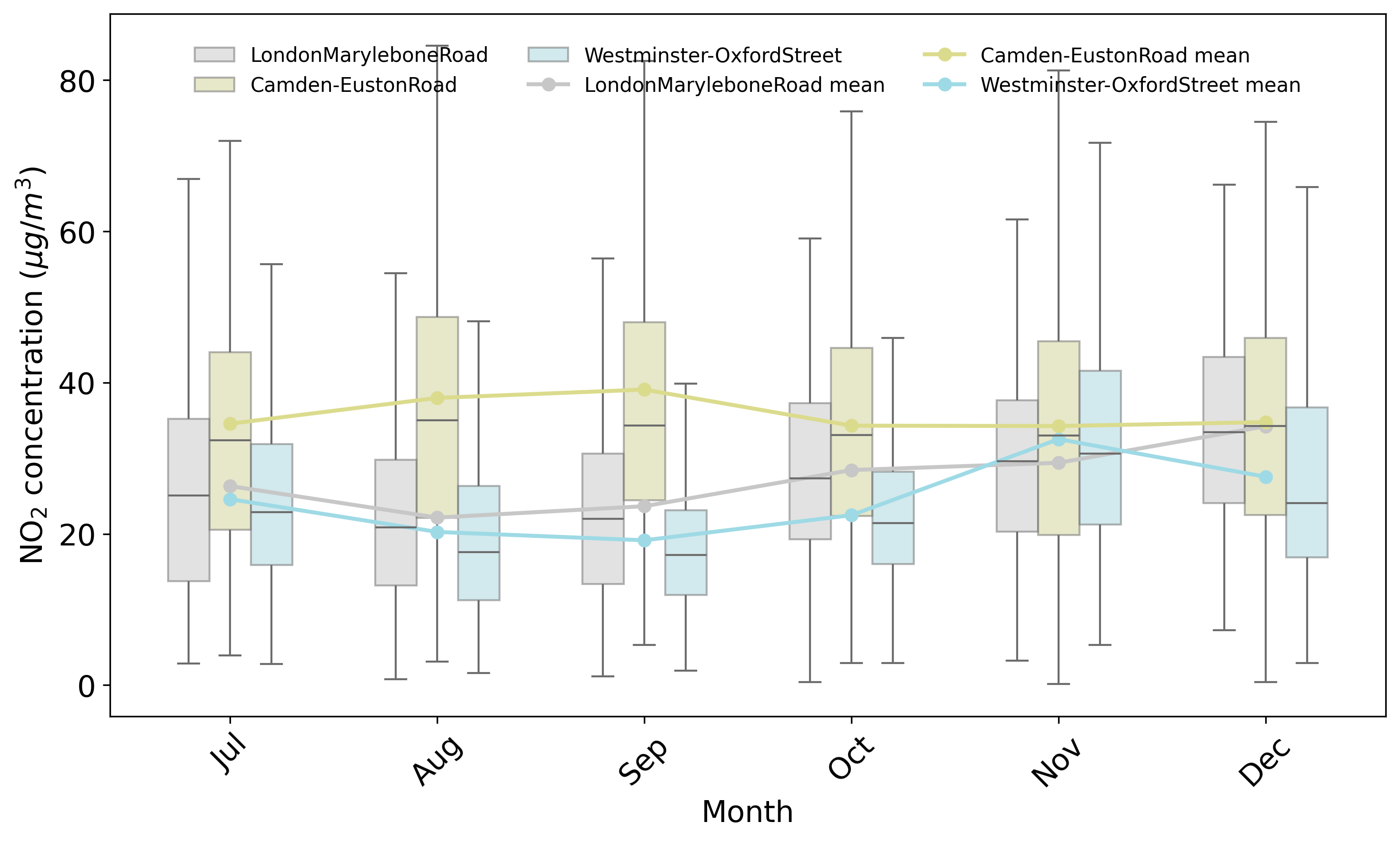
Figure 10 presents the distribution of pollutant concentrations at both the validation and training stations, illustrating the similarity of the pollutant patterns for this analysis. Figure 11 displays the monthly distribution of NO2 concentrations across Marylebone Road and the validation stations, while Figure 12 presents the mean hourly NO2 concentrations during the study period.

To quantify the performance degradation associated with applying a model trained at one monitoring location to a different site, we produce five NO2 estimates in the following configurations:
- •
Local models: the machine-learning models were trained independently for each validation station following the same methodology described in Section 2.3.
- •
Cross-site models: the models trained using data from Marylebone Road were applied to the data from each validation station.
- •
Interpolation methods: for comparison, NO2 estimates were also obtained for the same timestamps using the two interpolation methods described in Section 3.2.
The observed NO2 concentrations were compared with the predictions generated by the local models, the cross-site model, and the interpolation methods using the same independent test set from the fifth chronological split to ensure a fair, paired comparison.
The local model for Oxford Street achieves RMSE improvements of 12.37% when comparing Scen 2 with Scen 1, 12.31% when comparing Scen 3 with Scen 1. For the Euston local model, the corresponding improvements are 2.77%, and 15.81% respectively. Notably, the Euston model under Scen 2 exhibits very little improvement from incorporating NO2 measurements from the nearest background monitoring station compared with using only the predictors available in Scen 1. However, increasing the predictor set to the complexity of Scen 3 yields an additional improvement of over 10%.
Table 8 presents the RMSE obtained for each station, scenario and method considered in the validation process, together with the performance degradation associated with using the cross-site model instead of the local model, Ridge regression, IDW and OK. The performance degradation is quantified using Equation (5), with the local model as the reference scenario (A) and the cross-site model as the alternative scenario (B). Then, positive values indicate a percentage increase in RMSE when using the cross-site model relative to the corresponding comparison method, representing a loss in predictive performance, whereas negative values indicate a percentage decrease in RMSE, representing a performance advantage of the cross-site model over the comparison method.
Oxford Street has a lower RMSE achieved by the local models (9.76 on average across the six scenarios), compared with 13.62 at Euston. However, the cross-site models achieve higher average RMSE values at Oxford Street (14.22 ) than at Euston (12.12 ). Indeed, when evaluated on a scenario-by-scenario basis, the cross-site models consistently produce higher RMSE values at Oxford Street than at Euston.
| Station | Scenario | RMSECs | RMSEL | RMSER | RMSEIDW | RMSEOK | Cs vs L (%) | Cs vs R (%) | Cs vs IDW (%) | Cs vs OK (%) |
| Euston | S1 | 12.59 | 14.33 | 14.39 | 18.67 | 16.09 | 12.14 | 12.51 | 32.57 | 21.74 |
| Euston | S1-noT | 13.58 | 12.84 | 13.09 | 18.67 | 16.09 | 5.76 | 3.74 | 27.26 | 15.58 |
| Euston | S2 | 12.24 | 13.20 | 13.85 | 18.67 | 16.09 | 7.27 | 11.62 | 34.44 | 23.91 |
| Euston | S2-noT | 12.67 | 13.11 | 12.10 | 18.67 | 16.09 | 3.36 | 4.71 | 32.14 | 21.24 |
| Euston | S3 | 10.60 | 15.28 | 12.62 | 18.67 | 16.09 | 30.63 | 16.01 | 43.22 | 34.11 |
| Euston | S3-noT | 11.03 | 12.98 | 10.03 | 18.67 | 16.09 | 15.02 | 9.97 | 40.92 | 31.43 |
| Oxford St | S1 | 15.19 | 10.74 | 12.48 | 13.01 | 13.12 | 41.43 | 21.71 | 16.76 | 15.76 |
| Oxford St | S1-noT | 15.62 | 11.42 | 13.38 | 13.01 | 13.12 | 36.78 | 16.74 | 20.06 | 19.04 |
| Oxford St | S2 | 13.31 | 9.01 | 9.36 | 13.01 | 13.12 | 47.72 | 42.20 | 2.31 | 1.43 |
| Oxford St | S2-noT | 14.02 | 9.88 | 10.41 | 13.01 | 13.12 | 41.90 | 34.68 | 7.76 | 6.84 |
| Oxford St | S3 | 13.32 | 8.24 | 9.31 | 13.01 | 13.12 | 61.65 | 43.07 | 2.38 | 1.51 |
| Oxford St | S3-noT | 13.87 | 9.30 | 9.55 | 13.01 | 13.12 | 49.14 | 45.24 | 6.61 | 5.70 |
Note: is the degradation percentage calculated using Equation (5), with the local model as the reference scenario (A) and the cross-site model as the alternative scenario (B). Hence, positive values indicate a percentage increase in RMSE for the cross-site model relative to the corresponding comparison method, whereas negative values indicate a percentage decrease relative to the comparison method, representing a performance advantage of the cross-site model.
On the other hand, at Euston Road, the cross-site model frequently achieve lower RMSE values than the locally trained models, Ridge regression, and both interpolation methods, with reductions ranging from 3.36% to 43.22%. The largest improvement relative to the local model is observed for Scen 3, where the RMSE decreased from 15.28 for the local model to 10.60 for the cross-site model. In contrast, at Oxford Street, the cross-site model generally shows a performance degradation relative to the comparison methods across all scenarios. Specifically, when compared with the locally trained model, increases in RMSE range from 36.78% to 61.65%.
The contrasting results between Euston Road and Oxford Street suggest that cross-site transferability is strongly dependent on the target location. Notably, the model trained at Marylebone Road outperforms the locally trained model at Euston Road in five of the six scenarios, showing that training a model directly at the target site does not necessarily guarantee superior performance on a future independent period. This may indicate that, for Euston Road, the relationships learned from the Marylebone Road data generalise better to the independent test period than those learned from the target-site training data, whereas the degradation observed at Oxford Street suggests that such transferability cannot be assumed across locations.
Although these findings cannot be generalised given the limited number of target sites, several factors may contribute to the observed differences in model transferability, including road characteristics (Marylebone Road, Oxford Street, and Euston Road have six, two, and five traffic lanes, respectively), vehicle fleet composition, traffic patterns, meteorological conditions, nearby pollution sources, and local urban characteristics. Although Oxford Street is approximately half as far from Marylebone Road as Euston Road, these results suggest that geographical proximity alone may not determine model transferability and that similarities between the source and target locations may also play an important role.
3.4 Statistical Analysis
Tables 9–11 summarise the paired 24-h block-bootstrap comparisons between scenarios with and without traffic-related variables, evaluated on the independent chronological test set. For each comparison, the percentage improvement (RMSE), as described in Equation (4), its 95% confidence interval, and the Holm-adjusted p-value are reported. Positive values of RMSE indicate that the inclusion of traffic-related variables reduced the RMSE. A value of Yes in the Significant improvement column indicates that the inclusion of traffic-related variables resulted in both a positive RMSE improvement and a statistically significant difference after Holm correction.
| Pollutant | Station | Best Model | (%) | 95% CI | Holm-Adjusted -Value | Significant Improvement |
| NO2 | Marylebone Road | XGB | 10.38 | [0.56, 16.70] | 0.058 | No |
| NO2 | Camden Kerbside | XGB | 1.46 | [0.37, 3.08] | 0.214 | No |
| NO2 | Putney High Street | XGB | 1.21 | [2.07, 4.57] | 0.471 | No |
| NO2 | Oxford Street | XGB | 5.95 | [0.89, 10.18] | 0.030 | Yes |
| NO2 | Euston Road | ETR | 11.61 | [21.48, 1.96] | 0.072 | No |
| O3 | Marylebone Road | LGBM | 5.79 | [10.71, 0.85] | 0.045 | No |
| PM10 | Marylebone Road | RF | 0.90 | [3.35, 1.09] | 1.000 | No |
| PM10 | Camden Kerbside | XGB | 7.14 | [4.39, 11.72] | 0.001 | Yes |
| PM10 | Putney High Street | RF | 0.33 | [1.88, 1.50] | 1.000 | No |
| PM2.5 | Marylebone Road | XGB | 3.64 | [8.61, 1.37] | 0.615 | No |
| PM2.5 | Camden Kerbside | XGB | 10.19 | [2.66, 16.92] | 0.032 | Yes |
Note: is defined in Equation (4), where A represents the scenario without traffic-related variables, and B represents the corresponding scenario including traffic-related variables. Positive values indicate that including traffic variables reduced the RMSE. A statistically significant improvement is reported as Yes only when and the Holm-adjusted -value is below 0.05.
| Pollutant | Station | Best Model | (%) | 95% CI | Holm-Adjusted -Value | Significant Improvement |
| NO2 | Marylebone Road | XGB | 9.28 | [2.62, 14.21] | 0.020 | Yes |
| NO2 | Camden Kerbside | XGB | 0.91 | [2.14, 3.91] | 0.555 | No |
| NO2 | Putney High Street | LGBM | 4.53 | [1.71, 7.78] | 0.007 | Yes |
| NO2 | Oxford Street | LGBM | 8.78 | [3.93, 12.98] | 0.002 | Yes |
| NO2 | Euston Road | XGB | 0.71 | [9.22, 7.36] | 0.873 | No |
| O3 | Marylebone Road | LGBM | 2.12 | [5.48, 1.62] | 0.233 | No |
| PM10 | Marylebone Road | LGBM | 0.26 | [1.18, 2.06] | 1.000 | No |
| PM10 | Camden Kerbside | XGB | 0.14 | [3.02, 1.45] | 0.875 | No |
| PM10 | Putney High Street | LGBM | 0.13 | [1.05, 0.70] | 1.000 | No |
| PM2.5 | Marylebone Road | RF | 1.32 | [4.20, 6.70] | 1.000 | No |
| PM2.5 | Camden Kerbside | ETR | 0.63 | [1.16, 2.61] | 0.500 | No |
| Pollutant | Station | Best Model | (%) | 95% CI | Holm-Adjusted -Value | Significant Improvement |
| NO2 | Marylebone Road | LGBM | 5.44 | [1.50, 10.59] | 0.093 | No |
| NO2 | Camden Kerbside | LGBM | 4.63 | [1.09, 8.11] | 0.043 | Yes |
| NO2 | Putney High Street | XGB | 6.86 | [4.08, 9.20] | ¡0.001 | Yes |
| NO2 | Oxford Street | XGB | 11.42 | [5.30, 17.34] | 0.002 | Yes |
| NO2 | Euston Road | LGBM | 17.67 | [31.94, 2.92] | 0.072 | No |
| O3 | Marylebone Road | XGB | 4.21 | [1.11, 6.64] | 0.027 | Yes |
| PM10 | Marylebone Road | XGB | 0.91 | [2.15, 3.83] | 1.000 | No |
| PM10 | Camden Kerbside | XGB | 0.88 | [0.81, 1.37] | 0.438 | No |
| PM10 | Putney High Street | RF | 0.68 | [2.45, 0.95] | 0.798 | No |
| PM2.5 | Marylebone Road | RF | 2.30 | [2.31, 7.09] | 1.000 | No |
| PM2.5 | Camden Kerbside | RF | 5.14 | [8.95, 2.07] | 0.032 | No |
In Scen 1, statistically significant improvements after including traffic-related variables are observed for NO2 at Oxford Street, PM10 at Camden Kerbside, and PM2.5 at Camden Kerbside, with RMSE reductions ranging from approximately 5.95% to 10.19%.
Scen 2 provides the most consistent benefit from incorporating traffic-related variables. Statistically significant RMSE reductions are obtained for NO2 at Marylebone Road, Putney High Street, and Oxford Street, ranging from approximately 4.53% to 9.28%. In contrast, no statistically significant improvements are observed for O3, PM10, or PM2.5.
In Scen 3, significant improvements are again observed for NO2, particularly at Camden Kerbside, Putney High Street, and Oxford Street, together with O3 at Marylebone Road, ranging from 4.63% to 11.42%. Conversely, the inclusion of traffic-related variables significantly degrades performance for PM2.5 at Camden Kerbside, while NO2 at Euston Road also exhibits a substantial RMSE increase.
Overall, the statistical analysis indicates that the predictive benefit of traffic-related variables is heterogeneous across pollutants, stations, and feature scenarios, rather than providing a uniform improvement across all cases. Improvements are concentrated mainly in NO2 predictions, particularly under Scen 2 and Scen 3, whereas PM10 shows only isolated gains and PM2.5 exhibits mixed behaviour, including one statistically significant deterioration. O3 shows a statistically significant improvement only at Marylebone Road under Scen 3; however, as this is the only traffic-type station where O3 measurements are available, this result cannot be generalised to other sites.
The statistically significant improvements identified in this study are associated with RMSE reductions of approximately 4.5–11.4%, indicating non-negligible improvements in predictive performance. Nevertheless, these benefits are not consistent across pollutants and sites, and statistically significant performance degradations are also observed in some cases. These results highlight the need for further research to identify the site characteristics and local conditions under which traffic-related data provide a meaningful predictive benefit.
4 Discussion
4.1 Understanding the Role of Traffic and Spatial Context
The performance of the models was evaluated by comparing the three base predictor sets (scenarios) with their corresponding configurations after removing the traffic-related variables to assess whether their inclusion is worthwhile in the design of air-quality monitoring systems. These findings extend those reported by ref. [45], in which only a configuration equivalent to Scen 1 was analysed, and by ref. [42], which compared scenarios with an increasing number of predictors, without isolating the specific contribution of traffic-related variables.
As expected, the contribution of traffic-related variables is found to be pollutant- and site-dependent, with greater improvements observed at some monitoring locations than at others.
It is reported in ref. [14] that PM2.5 was heavily influenced by the traffic information represented as traffic emissions and speed, while NO2 showed better results when traffic was represented as vehicle counts. In contrast, ref. [42] used vehicle counts as a traffic descriptor, and there were no significant improvements reported in the RMSE of PM2.5 and PM10 estimates when traffic information was incorporated alongside meteorological variables and data from one air-quality monitoring station (the equivalent of Scen 2 in this study). Instead, the greatest contribution of traffic data was observed for NO2 prediction. In the present study, NO2 exhibited the greatest improvement from incorporating traffic variables based on travel time and speed, showing the highest average RMSE improvement across the three scenarios. In contrast, PM10, PM2.5, and O3 showed heterogeneous responses to the inclusion of traffic-related variables, with RMSE improvements in some scenarios and performance deterioration in others.
One possible explanation for why traffic-related variables did not improve O3 prediction in the simpler scenarios to the same extent as for NO2 could be that O3 is a secondary pollutant, and traffic variables therefore do not directly represent its formation processes. Interestingly, the contribution of traffic-related variables became beneficial under Scen 3, where measurements of pollutants involved in O3 chemistry, including NO2, NO, and NO as NO2, were also available as predictors. This may indicate that traffic information becomes more informative for O3 prediction when considered together with variables related to its photochemical formation and titration processes. Nevertheless, O3 was evaluated at only one station, which again limits the interpretation of these results.
Similar to the conclusions in ref. [42], in this study, when comparing predictive performance across scenarios, the inclusion of pollutant measurements from nearby stations also led to lower RMSE values than those obtained using traffic, temporal, and meteorological variables alone.
The SHAP analysis conducted in the present study showed that, at least for NO2 and O3, traffic-related variables played an important role in prediction, in some cases even greater than that of other pollutants measured at auxiliary stations. Therefore, as future work, it would be worthwhile to investigate whether some pollutants measured at auxiliary stations could be excluded from Scen 3 in order to reduce the data requirement associated with predicting NO2 or O3, once measurements of the same pollutant from nearby stations, together with local meteorological and traffic information, are already available. In contrast, for PM2.5, traffic-related variables did not have an impact on improving the predictions; in some cases, they even produced worse results, suggesting that, rather than contributing useful information, they may introduce noise into the modelling process.
4.2 Data Requirement–Performance Trade-Offs in Monitoring Design
In ref. [42], a configuration comparable to Scen 1 without traffic was found to perform worse than Scen 3 with traffic. Similarly, in the present study, Scen 3 outperformed Scen 1 across all analysed locations and pollutants. However, the comparison between Scen 3 and Scen 2 showed performance deterioration in some cases and only small improvements in others, highlighting that differences in model performance between scenarios should also be evaluated in terms of data requirement–performance trade-offs. This involves assessing not only the contribution of traffic-related variables but also whether the additional information required from multiple air-quality monitoring stations provides sufficient predictive improvement to justify the increased data requirements.
For PM10 estimation at the three analysed sites, the RMSE improvement obtained when moving from measurements from one neighbouring monitoring station (Scen 2) to measurements from four neighbouring stations (Scen 3) was below 5.37%, including one case of performance deterioration. For PM2.5, both analysed cases showed an increase in RMSE when incorporating data from the additional neighbouring stations. These results indicate that increasing the amount of monitoring-station information available to the model does not necessarily translate into better predictive performance.
The results from the validation experiment suggest that cross-site models may represent a practical alternative for extending air-quality estimation to some locations. However, given the limited number of cases analysed, it is not possible to identify which characteristics of the target and training locations may be relevant to successful model transferability. Although some degradation in performance relative to locally trained models may be expected, cross-site models can, in some cases, provide estimates with a reasonable degree of accuracy. Consequently, the proposed approach may contribute to improving access to air-quality information in areas where monitoring stations are unavailable or sparsely distributed, but where traffic and meteorological data can be obtained remotely through publicly available or commercial data services.
These results are not intended to suggest that the proposed approach can replace fixed-site air-quality monitoring networks, which, as discussed previously, remain the most reliable source of accurate pollutant measurements. Rather, the proposed framework aims to complement existing monitoring infrastructure by exploiting the available information from neighbouring monitoring stations together with traffic, temporal, and meteorological variables for air pollutant estimation.
4.3 Scalability and Spatial Deployment Considerations
The proposed framework relies on already existing infrastructure and does not require the installation of a new physical monitoring station. Nevertheless, acquiring data through commercial API services presents certain limitations. In the case of commercial providers, the number of free API requests per day is typically restricted to a relatively small amount, whereas subscriptions to paid plans are limited by institutional budgets. Under paid schemes, pricing depends on both the number of queried locations and the sampling frequency requested, with traffic-related data being particularly expensive and not obviously useful in terms of predictive value for air pollution estimation.
Hence, in operational settings, especially for practical large-scale deployment, the framework would require careful query-point selection for traffic and meteorological data acquisition. Therefore, future work should investigate optimal spatial querying strategies capable of identifying representative urban locations while minimising operational costs. Potential approaches may include Voronoi-based spatial partitioning, minimum-distance criteria between sampled locations, or spatial coverage optimisation methods considering road-network segmentation and urban morphology.
5 Conclusions
This work contributes to a growing body of evidence supporting the use of remote, commercially accessible traffic data as a meaningful input for ML-based urban air quality modelling. By systematically evaluating the contribution of traffic information across six predictor scenarios and five target locations in London, we reach conclusions that are relevant both to the predictive modelling literature and to practitioners involved in air quality monitoring network design.
The central finding of this study is that traffic-related information, such as speed and travel time, together with meteorological data, can provide additional predictive value for the estimation of NO2, O3, and PM10. The SHAP analysis revealed that traffic-related variables can contribute at a level comparable to, and in some cases greater than, measurements of the target pollutant obtained from neighbouring monitoring stations. This behaviour was particularly evident under Scen 2 at Marylebone Road and Putney High Street, where the contribution of traffic-related variables was similar to that of the nearest auxiliary-station NO2 measurements. Furthermore, under Scen 3 for NO2 prediction, traffic-related variables ranked above auxiliary pollutant measurements (aside from NO2) in terms of feature importance across the three stations considered in the main analysis. These findings are further supported by the Euston validation experiment, where incorporating NO2 measurements from the nearest monitoring station (Scen 2) provided only a marginal improvement over the traffic-, temporal-, and meteorology-based configuration (Scen 1), suggesting that traffic-state information may partially compensate for the absence of nearby air-quality observations under certain urban conditions.
The results from the validation experiment suggest that cross-site models can, in some cases, provide a practical alternative for locations where historical air-pollution measurements are unavailable but real-time traffic, temporal, and meteorological data can be obtained. Although these results cannot be generalised to other sites, performance degradation relative to locally trained models was observed in this study, ranging from 5.76% to 61.65% across the evaluated scenarios. Conversely, some scenarios showed improved performance, with improvements ranging from 3.36% to 30.63%. The resulting prediction errors remained within a range that may still be useful for some air-quality assessment applications, for example, at locations lacking monitoring infrastructure.
Nevertheless, given the limited number of sites analysed, it is not possible to determine which characteristics of the source and target locations favour successful model transferability. The observed results suggest that geographical proximity alone may not be sufficient and that factors such as urban morphology, road characteristics, nearby emission sources, and local environmental conditions may also be relevant. Consequently, locally trained models remain preferable whenever sufficient historical observations are available, whereas cross-site models may offer a valuable alternative in data-scarce environments.
A second contribution is methodological: the combination of a scenario-based ablation design with four tree-based ensemble models with classical interpolation and regression baselines enables a controlled decomposition of information gain that has been absent from prior comparative studies. Unlike works that evaluate traffic as a binary predictor (present or absent) this framework quantifies how the relative importance of traffic shifts as the information environment changes, offering a transferable evaluation protocol for future studies. By using this framework, we found that traffic data can provide valuable complementary information, particularly in environments where traffic is a predominant source of pollution. Nevertheless, its contribution was highly context-dependent, and pollutant measurements from traffic and background stations, together with meteorological variables, generally exhibited greater predictive value and feature importance.
From a practical perspective, the proposed framework relies on publicly accessible or commercially available datasets that offer free request allowances, although subject to daily or monthly request limits. This allows the framework to be reproduced and deployed without the need for additional sensing infrastructure.
The reliance on these data sources (e.g., UK-AIR, OpenWeather, and TomTom) makes the proposed pipeline potentially reproducible in cities where equivalent air-quality data and commercial traffic and meteorological data services are available, reducing the barriers to deploying virtual air-quality monitoring systems in low- and middle-income urban contexts.
It is important to note that the London case study was conducted using monitoring stations located within the Ultra Low Emission Zone (ULEZ). Consequently, traffic composition, fleet characteristics, and pollutant concentrations may differ from other cities operating under different traffic management and emission-regulation frameworks.
Three directions for future work are identified in order to improve the generalisability of the study: (i) validation of the framework in other cities with different atmospheric dynamics, traffic compositions, and climate conditions; (ii) integration of spatio-temporal deep learning architectures that can model dependencies across the monitoring network dynamically; and (iii) exploration of emission inventory features at multi-source sites to extend the applicability of the approach beyond traffic-dominated corridors.
Future work should also extend the cross-site transferability study. The cross-site transferability analysis was limited by data availability, which meant that transferability could only be assessed at two additional stations and only for NO2. Given this small sample, future efforts should evaluate transferability across a larger number of sites and for multiple pollutants.
The study period was constrained by time and resource limitations associated with the real-time collection of traffic data through the TomTom API, resulting in a dataset covering June to December. Given the relationship between O3 and temperature and humidity, its seasonal cycle [11] could not be fully captured within the study period, limiting the generalisability of its predictions across the year. Therefore, in future research it would be beneficial to extend the study period to the whole year so that we can validate model performance over the full yearly cycle.
The conclusions of this study, beyond the specific variables analysed, suggest that incorporating relevant information directly related to pollution sources can improve pollutant prediction, enabling the approximation of their influence without the need for additional sensors or extensive monitoring networks. Hence, consideration could also be given to incorporating information related to other types of pollution sources, as well as additional data formats such as satellite imagery of atmospheric conditions, traffic flow video data, or quantitative descriptors of the surrounding environment, including the presence of green areas, nearby industrial facilities, and other urban characteristics.
5.1 Data Availability
Restrictions apply to the availability of these data. Traffic and meteorological data providers do not permit the large-scale redistribution of data downloaded directly from their APIs. Raw traffic data were acquired in real time through the TomTom Flow Segment Data API [47] under its free-access scheme. Meteorological data can be reproduced by querying the OpenWeather One Call API 3.0 [37] under the user’s own credentials and licensing conditions, although free access is subject to a limited number of daily requests. Historical air pollution data are publicly available from the official UK government repository in [12]. The code is available on Zenodo at DOI: https://zenodo.org/records/21863941.
5.2 Acknowledgements
We thank our institutions, the Instituto Politécnico Nacional (IPN) and Queen Mary University of London (QMUL), for enabling this collaboration through the provision of IT facilities and access to invaluable expertise, particularly from Daohai Li and Alex Owen at QMUL. We also gratefully acknowledge the sponsors who supported this collaboration, such as Fundación Politécnico and COFAA-IPN.
5.3 Author contributions
Conceptualisation: M.B., V.L.-S., J.R. Data Curation: V.L.-S. Formal Analysis: M.B., V.L.-S., J.R. Funding Acquisition: A.A., M.B., V.L.-S., M.S.-P. Investigation: M.B., V.L.-S., J.R. Methodology: M.B., V.L.-S., J.R. Project Administration: M.B. Resources: A.A., M.B., M.S.-P. Software: V.L.-S. Supervision: A.A., M.B., M.S.-P. Validation: V.L.-S. Visualisation: V.L.-S. Writing—Original Draft Preparation: M.B., V.L.-S. Writing—Review & Editing: A.A., M.B., V.L.-S., J.R., M.S.-P. All authors have read and agreed to the published version of the manuscript
5.4 Funding
A.A. received funding from the SIP-IPN under grant agreement No. SIP20250146, SIP-2284 and ProRed 2026-0060. M.B. received funding from the Science and Technology Facilities Council (STFC) Impact Acceleration Account. V.L.-S. receives financial support from the Secretaría de Ciencia, Humanidades, Tecnología e Innovación (SECIHTI) under grant 960525; the Fundación Politécnico, IPN and QMUL through the dual doctoral programme between the IPN and QMUL; and the Comisión de Operación y Fomento de Actividades Académicas (COFAA-IPN). J.R. receives funding from QMUL via a Principal’s PhD Studentship. M.S.-P. has received funding from the SIP-IPN under grants IND-2026-0524, SECTEI/084/2023 and CM-SECTEI/040/2025. M.S.-P. and V.L.-S. received funding from the SIP-IPN under grant 2024-A175.
5.5 Competing interests
The authors declare no conflicts of interest.
References
- [1] (2021) Air quality changes in cities during the covid-19 lockdown: a critical review. Atmospheric Research 264, pp. 105823. External Links: ISSN 0169-8095, Document Cited by: §1.
- [2] (2023) Air pollution and inequalities london update 2023. Note: Available online: https://www.london.gov.uk/programmes-strategies/environment-and-climate-change/environment-and-climate-change-publications/air-pollution-and-inequalities-london-update-2023(accessed on 13 May 2026). Cited by: §1.
- [3] (2019) Optuna: a next-generation hyperparameter optimization framework. In Proceedings of the 25th ACM SIGKDD International Conference on Knowledge Discovery & Data Mining, KDD ’19, New York, NY, USA, pp. 2623–2631. External Links: ISBN 9781450362016, Link, Document Cited by: §2.3.
- [4] (2019) Modeling of CO emissions from traffic vehicles using artificial neural networks. Applied Sciences (Switzerland) 9 (2), pp. 313. External Links: Document Cited by: §1, §1.
- [5] (2026) Tackling air quality with sapiens. Note: arXiv:2601.23215, https://arxiv.org/abs/2601.23215accessed 28 Jul 2026 External Links: 2601.23215 Cited by: §1.
- [6] (2001) Random forests. Machine Learning 45 (1), pp. 5–32. External Links: Document Cited by: §2.3.
- [7] (2025) Estimating pm2.5 concentrations at public schools in north carolina using multiple data sources and interpolation methods. Scientific Reports 15, pp. 42600. External Links: Document, Link Cited by: §2.4, §2.4.
- [8] (2010) On over-fitting in model selection and subsequent selection bias in performance evaluation. Journal of Machine Learning Research 11, pp. 2079–2107. Cited by: §2.1.
- [9] (2016) XGBoost: a scalable tree boosting system. In KDD ’16: Proceedings of the 22nd ACM SIGKDD International Conference on Knowledge Discovery and Data Mining, KDD ’16, New York, NY, USA, pp. 785–794. External Links: ISBN 9781450342322, Link, Document Cited by: §2.3.
- [10] (2025) Air quality strategy 2025-2030. City of London Corporation, London, United Kingdom. Note: Available online: https://www.cityoflondon.gov.uk/assets/Services-Environment/city-of-london-air-quality-strategy-2025-2030.pdf(accessed on 11 May 2026). Cited by: §1.
- [11] (2026) Accredited official statistics: ozone (o3). Note: Available online: https://www.gov.uk/government/statistics/air-quality-statistics/concentrations-of-ozone(accessed on 04 Aug 2026). Cited by: §5.
- [12] (2026) UK-air: air quality data archive. Note: Available online: https://uk-air.defra.gov.uk/data/(accessed on 13 May 2026). Cited by: §2.1, §5.1.
- [13] (2026) UK-air: site environment types. Note: Available online: https://uk-air.defra.gov.uk/networks/site-types(accessed on 13 May 2026). Cited by: §1, §2.1.
- [14] (2025) Real-time air quality prediction using traffic videos and machine learning. Transportation Research Part D: Transport and Environment 142, pp. 104688. External Links: ISSN 1361-9209, Document, Link Cited by: §1, §1, §1, §2.2, §2.3, §4.1.
- [15] (2025) Advancements in machine learning for spatiotemporal urban on-road traffic-air quality study: a review. Atmospheric Environment 346, pp. 121054. External Links: ISSN 1352-2310, Document, Link Cited by: §1, §2.3.
- [16] (2023) Europe’s air quality status 2023. Note: Available online: https://www.eea.europa.eu/publications/europes-air-quality-status-2023(accessed on 11 May 2026). Cited by: §1.
- [17] (2022) Geospatial clustering and hot spot detection of malaria incidence in bahawalpur district of pakistan. GeoJournal 87, pp. 4791–4806. External Links: Document, Link Cited by: §2.4.
- [18] (2006) Extremely randomized trees. Machine Learning 63 (1), pp. 3–42. External Links: Document Cited by: §2.3.
- [19] (2020) Air quality in london 2016–2020. Greater London Authority. Note: Available online: https://www.london.gov.uk/sites/default/files/air_quality_in_london_2016-2020_october2020final.pdf(accessed on 27 Nov 2025). Cited by: §1.
- [20] (1970) Ridge regression: biased estimation for nonorthogonal problems. Technometrics 12 (1), pp. 55–67. External Links: Document, Link, https://doi.org/10.1080/00401706.1970.10488634 Cited by: §2.3.
- [21] (2025) Transforming cctv cameras into sensors at city scale for adaptive policymaking. Scientific Reports 15, pp. 3640. External Links: Document, Link Cited by: §1, §1.
- [22] (2020) Feature relevance quantification in explainable ai: a causal problem. In Proceedings of the Twenty Third International Conference on Artificial Intelligence and Statistics, S. Chiappa and R. Calandra (Eds.), Proceedings of Machine Learning Research, Vol. 108, Norfolk, MA, USA, online, pp. 2907–2916. External Links: Link Cited by: §2.3.
- [23] (2024) Forecasting urban air pollution using multi-site spatiotemporal data fusion method (geo-bilstma). Atmospheric Pollution Research 15 (6), pp. 102107. External Links: ISSN 1309-1042, Document, Link Cited by: §2.4.
- [24] (2024) Evaluating traditional versus ensemble machine learning methods for predicting missing data of daily pm10 concentration. Atmospheric Pollution Research 15 (5), pp. 102063. External Links: ISSN 1309-1042, Document, Link Cited by: §2.3.
- [25] (2019) A random forest partition model for predicting NO2 concentrations from traffic flow and meteorological conditions. Science of The Total Environment 651, pp. 475–483. External Links: ISSN 0048-9697, Document Cited by: §1, §1.
- [26] (2025) How much does traffic flow modification change air quality? scenario-based study. Science of The Total Environment 1001, pp. 180560. External Links: ISSN 0048-9697, Document, Link Cited by: §1, §1.
- [27] (2017) LightGBM: a highly efficient gradient boosting decision tree. In Advances in Neural Information Processing Systems, I. Guyon, U. V. Luxburg, S. Bengio, H. Wallach, R. Fergus, S. Vishwanathan, and R. Garnett (Eds.), Vol. 30, pp. 3146–3154. External Links: Link, ISBN 9781510860964 Cited by: §2.3.
- [28] (2026) A review on air pollution prediction using artificial intelligence. IEEE Access 14 (), pp. 26024–26040. External Links: Document Cited by: §2.3.
- [29] (2019) Predictive analytics of pm10 concentration levels using detailed traffic data. Transportation Research Part D: Transport and Environment 67, pp. 131–141. External Links: ISSN 1361-9209, Document, Link Cited by: §1, §1.
- [30] (2020) Exploring the relationship between air pollution and meteorological conditions in china under environmental governance. Scientific Reports 10, pp. 14518. External Links: Document, Link Cited by: §1.
- [31] (2020) From local explanations to global understanding with explainable ai for trees. Nature Machine Intelligence 2 (1), pp. 56–67. External Links: Document Cited by: §2.3.
- [32] (2017) A unified approach to interpreting model predictions. In Proceedings of the 31st International Conference on Neural Information Processing Systems, NIPS’17, Red Hook, NY, USA, pp. 4768–4777. External Links: ISBN 9781510860964 Cited by: §2.3.
- [33] (2025) PM2.5 concentration prediction using machine learning algorithms: an approach to virtual monitoring stations. Scientific Reports 15, pp. 8076. External Links: Document, Link Cited by: §1, §2.3.
- [34] (2026) Monitoring urban air quality in lahore: a combined approach using ground measurements and sentinel-5p data. International Journal of Environmental Science and Technology 23, pp. 207. External Links: Document, Link Cited by: §2.4.
- [35] (2022) GeoStat-framework/pykrige: v1.7.0. Zenodo. Note: Available online: https://zenodo.org/records/7008206Version 1.7.0, Zenodo (accessed on 13 May 2026). Cited by: §2.4.
- [36] (2025) Using gaussian processes for spatial prediction of pm2.5 concentration based on calibrated data from distributed low-cost sensor networks. Environmental Data Science 4, pp. e52. External Links: Document Cited by: §2.4.
- [37] (2026) One call api 3.0. Note: Available online: https://openweathermap.org/api/one-call-3?collection=one_call_api_3.0(accessed on 13 May 2026). Cited by: §2.1, §5.1.
- [38] (2025) The effect of the ultra-low emission zone on PM2.5 concentration in Seoul, South Korea. Atmospheric Environment 340, pp. 120908. External Links: ISSN 1352-2310, Document, Link Cited by: §1.
- [39] (2011) Scikit-learn: machine learning in python. Journal of Machine Learning Research 12 (85), pp. 2825–2830. External Links: Link Cited by: §2.1.
- [40] (2023) Short-term air pollution forecasting using embeddings in neural networks. Atmosphere 14 (2), pp. 298. External Links: Document Cited by: §1.
- [41] (2020) Effect of road traffic on air pollution. experimental evidence from covid-19 lockdown. Sustainability 12 (21), pp. 8984. External Links: Document Cited by: §1.
- [42] (2023) Air pollution prediction using machine learning techniques – an approach to replace existing monitoring stations with virtual monitoring stations. Atmospheric Environment 310, pp. 119987. External Links: ISSN 1352-2310, Document, Link Cited by: §1, §1, §1, §2.1, §2.2, §2.3, §2.5, §4.1, §4.1, §4.1, §4.2.
- [43] (2023) Spatial-temporal prediction of air quality by deep learning and kriging interpolation approach. EAI Endorsed Transactions on Scalable Information Systems 10 (5), pp. 1–14. External Links: Link, Document Cited by: §2.4.
- [44] (2026) Cross validation on time series data. Note: Available online: https://scikit-learn.org/stable/modules/cross_validation.html#cross-validation-of-time-series-data(accessed on 13 May 2026). Cited by: §2.1.
- [45] (2022) Effect of traffic data set on various machine-learning algorithms when forecasting air quality. Journal of Engineering, Design and Technology 22 (3), pp. 1030–1056. External Links: ISSN 1726-0531, Document, Link Cited by: §1, §1, §1, §2.2, §2.3, §2.5, §4.1.
- [46] (2024) Analysis of local and regional contributions of oxidant (ox = o3 + no2) levels based on monitoring data: a review. International Journal of Environmental Science and Technology 21, pp. 8211–8230 (english). External Links: Document, Link Cited by: §1.
- [47] (2026) Flow segment data. Note: Available online: https://developer.tomtom.com/traffic-api/documentation/tomtom-maps/traffic-flow/flow-segment-data(accessed on 13 May 2026). Cited by: §2.1, §5.1.
- [48] (20 May 2026-05) Clean air act requirements and history.. Note: Available online: https://www.epa.gov/clean-air-act-overview/clean-air-act-requirements-and-history(Accessed on 22 June 2026). Cited by: §1.
- [49] (2026) Criteria air pollutants. Note: Available online: https://www.epa.gov/criteria-air-pollutants(accessed on 13 May 2026). Cited by: §1.
- [50] (2006) Bias in error estimation when using cross-validation for model selection. BMC Bioinformatics 7 (1), pp. 91. External Links: Document Cited by: §2.1.
- [51] (2020) COVID-19 lockdowns cause global air pollution declines. Proceedings of the National Academy of Sciences of the United States of America 117 (32), pp. 18984–18990. External Links: Document Cited by: §1.
- [52] (2026) Air quality assessment and spatiotemporal dynamics of pm10, nox, and so2 in navi mumbai, india (2014–2023): a gis-based weighted overlay approach. CLEAN – Soil, Air, Water 54 (3), pp. e70127. External Links: Document, Link Cited by: §2.4.
- [53] (2022) Network approach reveals the spatiotemporal influence of traffic on air pollution under covid-19. Chaos 32 (4), pp. 041106. External Links: Document Cited by: §1.
- [54] Types of pollutants. Note: Available online: https://www.who.int/teams/environment-climate-change-and-health/air-quality-and-health/health-impacts/types-of-pollutants(accessed on 22 June 2026). Cited by: §1.
- [55] (2021) WHO global air quality guidelines: particulate matter (PM2.5 and PM10), ozone, nitrogen dioxide, sulfur dioxide and carbon monoxide. Note: Available online: https://www.who.int/publications/i/item/9789240034228(accessed on 11 May 2026). Cited by: §1.
- [56] (2024) Ambient (outdoor) air pollution. Note: Available online: https://www.who.int/news-room/fact-sheets/detail/ambient-(outdoor)-air-quality-and-health(accessed on 11 May 2026). Cited by: §1.
- [57] (2025) Air pollution (overview). Note: Available online: https://www.who.int/health-topics/air-pollution##tab=tab_1(accessed on 11 May 2026). Cited by: §1.
- [58] (2020) A traffic-based method to predict and map urban air quality. Applied Sciences (Switzerland) 10, pp. 2035. External Links: Document, ISSN 20763417 Cited by: §1, §1.
Appendix A Supplementary Material
The figures part of the supplementary material are available as ancillary files accompanying this submission. The supplementary material provides information for all monitoring stations considered in this study, including the validation stations that were analysed separately from the main experimental dataset.
The figures in the ancillary material are listed below.
- Figure S1
-
corresponds to the file OpenWeather_validation_temperature_wind.png. Comparison of OpenWeather meteorological data with observations from the air quality monitoring stations at Camden Kerbside and Marylebone Road.
- Figure S2
-
corresponds to the file Correlation_Matrix_LondonMaryleboneRoad.png. Correlation matrix between temporal, remotely acquired traffic and meteorological variables, and criteria pollutants measured at the London Marylebone Road station.
- Figure S3
-
corresponds to the file Correlation_Matrix_Wandsworth-PutneyHighStreet.png. Correlation matrix between temporal, remotely acquired traffic and meteorological variables, and criteria pollutants measured at the Wandsworth – Putney High Street station.
- Figure S4
-
corresponds to the file Correlation_Matrix_CamdenKerbside.png. Correlation matrix between temporal, remotely acquired traffic and meteorological variables, and criteria pollutants measured at the Camden Kerbside station.
- Figure S5
-
corresponds to the file Correlation_Matrix_Westminster-OxfordStreet.png. Correlation matrix between temporal, remotely acquired traffic and meteorological variables, and criteria pollutants measured at the Westminster – Oxford Street station.
- Figure S6
-
corresponds to the file Correlation_Matrix_Camden-EustonRoad.png. Correlation matrix between temporal, remotely acquired traffic and meteorological variables, and criteria pollutants measured at the Camden – Euston Road station.
- Figure S7
-
corresponds to the file time_series_observed_ML_Ridge_PM10.png. Observed and predicted concentrations on the final chronological test set, comparing the best-performing tree-based model with Ridge regression.
- Figure S8
-
corresponds to the file time_series_observed_ML_Ridge_NO2.png. Observed and predicted concentrations on the final chronological test set, comparing the best-performing tree-based model with Ridge regression.
- Figure S9
-
corresponds to the file time_series_observed_ML_Ridge_O3.png. Observed and predicted concentrations on the final chronological test set, comparing the best-performing tree-based model with Ridge regression.
- Figure S10
-
corresponds to the file time_series_observed_ML_Ridge_PM25.png. Observed and predicted concentrations on the final chronological test set, comparing the best-performing tree-based model with Ridge regression.
| Station | Pollutant | Pollution | Traffic | Pollution + traffic | Weather | Bkg0 | Bkg1 | Trf0 | Trf1 | Final merge |
| Euston Road | NO2 | 4152 | 4510 | 3747 | 4151 | 4151 | 4151 | 4151 | 4151 | 3747 |
| Camden Kerbside | NO2 | 4152 | 4706 | 3943 | 4152 | 4151 | 4151 | 4151 | 4151 | 3943 |
| Camden Kerbside | PM10 | 4152 | 4706 | 3943 | 4152 | 4151 | 4151 | 4151 | 4151 | 3943 |
| Camden Kerbside | PM25 | 4152 | 4706 | 3943 | 4152 | 4151 | 4151 | 4151 | 4151 | 3943 |
| Marylebone Road | NO2 | 4152 | 4707 | 3944 | 4152 | 4151 | 4151 | 4151 | 4151 | 3944 |
| Marylebone Road | O3 | 4152 | 4707 | 3944 | 4152 | 4151 | 4151 | 4151 | 4151 | 3944 |
| Marylebone Road | PM10 | 4152 | 4707 | 3944 | 4152 | 4151 | 4151 | 4151 | 4151 | 3944 |
| Marylebone Road | PM25 | 4152 | 4707 | 3944 | 4152 | 4151 | 4151 | 4151 | 4151 | 3944 |
| Putney High Street | NO2 | 4152 | 4510 | 3747 | 4152 | 3747 | 4151 | 4151 | 4151 | 3747 |
| Putney High Street | PM10 | 4152 | 4510 | 3747 | 4152 | 3747 | 4151 | 4151 | 4151 | 3747 |
| Oxford Street | NO2 | 4152 | 4510 | 3747 | 4152 | 4151 | 4151 | 4151 | 4151 | 3747 |
Note: Pollution and traffic indicate the number of observations available from the target monitoring station and hourly aggregated traffic data, respectively. Bkg0 and Bkg1 denote the two nearest background stations, while Trf0 and Trf1 denote the two nearest traffic stations. Final merge indicates the number of observations remaining after merging all data sources by timestamp.
| Station | Pollutant | After cleaning | Missing target | After target removal | Missing predictors | Rows with missing | Interpolated values | Rows with missing (%) | Missing values interpolated (%) |
| Euston Road | NO2 | 3747 | 515 | 3232 | 424 | 264 | 236 | 8.17 | 55.66 |
| Camden Kerbside | NO2 | 3943 | 31 | 3912 | 866 | 517 | 443 | 13.22 | 51.15 |
| Camden Kerbside | PM10 | 3943 | 103 | 3840 | 871 | 503 | 449 | 13.10 | 51.55 |
| Camden Kerbside | PM25 | 3943 | 74 | 3869 | 880 | 507 | 464 | 13.10 | 52.73 |
| Marylebone Road | NO2 | 3944 | 53 | 3891 | 612 | 336 | 304 | 8.64 | 49.67 |
| Marylebone Road | O3 | 3944 | 334 | 3610 | 560 | 316 | 293 | 8.75 | 52.32 |
| Marylebone Road | PM10 | 3944 | 243 | 3701 | 570 | 311 | 271 | 8.40 | 47.54 |
| Marylebone Road | PM25 | 3944 | 234 | 3710 | 542 | 295 | 274 | 7.95 | 50.55 |
| Putney High Street | NO2 | 3747 | 10 | 3737 | 1151 | 718 | 456 | 19.21 | 39.62 |
| Putney High Street | PM10 | 3747 | 28 | 3719 | 1139 | 712 | 443 | 19.14 | 38.89 |
| Oxford Street | NO2 | 3747 | 90 | 3657 | 661 | 385 | 323 | 10.53 | 48.87 |
Note: Missing target indicates observations removed because the target pollutant concentration was unavailable. Missing predictors indicates the total number of missing predictor values before interpolation, whereas Rows with missing indicates the number of observations containing at least one missing predictor. Interpolated values indicates the number of unique missing predictor values recovered by temporal interpolation in at least one of the cross-validation partitions in which they occurred. Rows with missing (%) indicates the proportion of rows containing at least one missing predictor value, whereas Missing values interpolated (%) indicates the proportion of missing predictor values recovered through interpolation relative to the total number of missing predictor values.
| Model | Hyperparameter | Search space | Scale / condition |
| RF | n_estimators | [200, 800], step 100 | integer |
| RF | max_depth | [4, 30] | integer |
| RF | min_samples_split | [2, 30] | integer |
| RF | min_samples_leaf | [1, 15] | integer |
| RF | max_features | {sqrt, log2, 0.3, 0.5, 0.7, 0.9} | categorical |
| RF | bootstrap | {True, False} | categorical |
| RF | ccp_alpha | [, ] | log-uniform |
| RF | max_samples | [0.50, 0.95] | if bootstrap = True |
| ETR | n_estimators | [200, 800], step 100 | integer |
| ETR | max_depth | [4, 35] | integer |
| ETR | max_leaf_nodes | [20, 300] | integer |
| ETR | min_samples_split | [2, 30] | integer |
| ETR | min_samples_leaf | [1, 15] | integer |
| ETR | max_features | {sqrt, log2, 0.3, 0.5, 0.7, 0.9} | categorical |
| ETR | bootstrap | {True, False} | categorical |
| ETR | ccp_alpha | [, ] | log-uniform |
| ETR | max_samples | [0.50, 0.95] | if bootstrap = True |
| LGBM | n_estimators | [300, 1500], step 100 | integer |
| LGBM | learning_rate | [, 0.08] | log-uniform |
| LGBM | num_leaves | [15, 255] | integer |
| LGBM | max_depth | [3, 12] | integer |
| LGBM | min_child_samples | [10, 120] | integer |
| LGBM | min_child_weight | [, 10] | log-uniform |
| LGBM | subsample | [0.50, 1.00] | uniform |
| LGBM | subsample_freq | [1, 10] | integer |
| LGBM | colsample_bytree | [0.50, 1.00] | uniform |
| LGBM | reg_alpha | [, 10] | log-uniform |
| LGBM | reg_lambda | [, 10] | log-uniform |
| LGBM | min_split_gain | [, 1] | log-uniform |
| XGB | n_estimators | [300, 1500], step 100 | integer |
| XGB | learning_rate | [, 0.08 | log-uniform |
| XGB | max_depth | [3, 12] | integer |
| XGB | min_child_weight | [1, 20] | log-uniform |
| XGB | gamma | [, 10] | log-uniform |
| XGB | subsample | [0.50, 1.00] | uniform |
| XGB | colsample_bytree | [0.40, 1.00] | uniform |
| XGB | colsample_bylevel | [0.40, 1.00] | uniform |
| XGB | reg_alpha | [, 10] | log-uniform |
| XGB | reg_lambda | [, 20] | log-uniform |
| XGB | grow_policy | {depthwise, lossguide} | categorical |
| XGB | booster | gbtree | fixed |
| Station | Variogram | Partial sill | Sill | Range (km) | Nugget |
| Marylebone Road | Spherical | 31.3479 | 34.4045 | 1.8608 | 3.0566 |
| Camden Kerbside | Spherical | 10.2275 | 13.8756 | 2.2328 | 3.6481 |
| Putney High Street | Exponential | 0.0011 | 42.7250 | 0.0373 | 42.7239 |
| Oxford Street | Spherical | 22.0926 | 31.0504 | 5.0849 | 8.9578 |
| Euston Road | Exponential | 62.5974 | 66.6085 | 0.0355 | 4.0111 |
| Pollutant | Station | Scenario | Best model | RMSE | MAE | |
| NO2 | Marylebone Road | S1 | XGB | 10.22 1.71 | 7.73 1.23 | 0.33 0.17 |
| NO2 | Marylebone Road | S1-noT | LGBM | 10.20 1.93 | 7.73 1.26 | 0.34 0.14 |
| NO2 | Marylebone Road | S2 | XGB | 9.17 1.30 | 6.85 0.86 | 0.47 0.07 |
| NO2 | Marylebone Road | S2-noT | ETR | 9.30 1.57 | 7.02 0.95 | 0.46 0.09 |
| NO2 | Marylebone Road | S3 | LGBM | 8.01 1.43 | 5.96 1.06 | 0.59 0.09 |
| NO2 | Marylebone Road | S3-noT | LGBM | 8.16 1.78 | 5.92 1.02 | 0.58 0.10 |
| NO2 | Camden Kerbside | S1 | XGB | 9.27 2.31 | 6.76 1.43 | 0.39 0.16 |
| NO2 | Camden Kerbside | S1-noT | XGB | 9.23 2.06 | 6.68 1.30 | 0.39 0.16 |
| NO2 | Camden Kerbside | S2 | XGB | 7.37 2.07 | 5.38 1.28 | 0.62 0.11 |
| NO2 | Camden Kerbside | S2-noT | LGBM | 7.48 2.11 | 5.43 1.41 | 0.60 0.13 |
| NO2 | Camden Kerbside | S3 | LGBM | 6.82 1.83 | 5.01 1.03 | 0.68 0.08 |
| NO2 | Camden Kerbside | S3-noT | LGBM | 6.80 1.83 | 4.88 1.01 | 0.68 0.08 |
| NO2 | Putney High Street | S1 | XGB | 9.13 1.01 | 6.99 0.95 | 0.56 0.05 |
| NO2 | Putney High Street | S1-noT | LGBM | 9.43 1.14 | 7.22 1.04 | 0.53 0.05 |
| NO2 | Putney High Street | S2 | LGBM | 8.24 1.57 | 6.20 1.45 | 0.64 0.11 |
| NO2 | Putney High Street | S2-noT | LGBM | 8.51 1.85 | 6.33 1.66 | 0.61 0.13 |
| NO2 | Putney High Street | S3 | XGB | 7.65 1.17 | 5.61 1.02 | 0.69 0.06 |
| NO2 | Putney High Street | S3-noT | LGBM | 7.81 1.32 | 5.66 1.13 | 0.68 0.07 |
| NO2 | Oxford Street | S1 | XGB | 10.16 2.35 | 7.83 1.73 | 0.13 0.15 |
| NO2 | Oxford Street | S1-noT | XGB | 10.44 2.55 | 8.05 1.79 | 0.08 0.19 |
| NO2 | Oxford Street | S2 | LGBM | 7.90 1.97 | 6.02 1.58 | 0.47 0.14 |
| NO2 | Oxford Street | S2-noT | LGBM | 8.09 2.17 | 6.18 1.73 | 0.44 0.18 |
| NO2 | Oxford Street | S3 | XGB | 6.99 1.58 | 5.33 1.14 | 0.57 0.16 |
| NO2 | Oxford Street | S3-noT | XGB | 7.40 1.56 | 5.58 1.12 | 0.50 0.23 |
| NO2 | Euston Road | S1 | ETR | 18.53 6.04 | 13.16 2.78 | 0.09 0.49 |
| NO2 | Euston Road | S1-noT | LGBM | 18.03 6.92 | 12.32 2.84 | 0.21 0.24 |
| NO2 | Euston Road | S2 | XGB | 17.91 5.91 | 12.33 2.43 | 0.16 0.43 |
| NO2 | Euston Road | S2-noT | RF | 17.30 7.13 | 11.40 2.91 | 0.28 0.26 |
| NO2 | Euston Road | S3 | LGBM | 15.69 6.84 | 9.96 2.40 | 0.43 0.17 |
| NO2 | Euston Road | S3-noT | RF | 15.75 7.05 | 9.72 2.57 | 0.43 0.19 |
| O3 | Marylebone Road | S1 | LGBM | 10.65 1.58 | 8.51 1.17 | 0.25 0.28 |
| O3 | Marylebone Road | S1-noT | LGBM | 11.09 1.71 | 8.90 1.34 | 0.15 0.44 |
| O3 | Marylebone Road | S2 | LGBM | 7.50 1.74 | 6.03 1.57 | 0.64 0.08 |
| O3 | Marylebone Road | S2-noT | LGBM | 7.85 1.46 | 6.35 1.34 | 0.59 0.14 |
| O3 | Marylebone Road | S3 | XGB | 6.46 1.73 | 5.23 1.65 | 0.74 0.06 |
| O3 | Marylebone Road | S3-noT | LGBM | 6.73 1.59 | 5.38 1.48 | 0.71 0.06 |
| PM10 | Marylebone Road | S1 | RF | 7.21 0.75 | 5.41 0.52 | 0.13 0.07 |
| PM10 | Marylebone Road | S1-noT | RF | 7.31 0.78 | 5.46 0.55 | 0.10 0.06 |
| PM10 | Marylebone Road | S2 | LGBM | 5.55 0.44 | 4.09 0.41 | 0.48 0.08 |
| PM10 | Marylebone Road | S2-noT | LGBM | 5.58 0.37 | 4.11 0.34 | 0.47 0.08 |
| PM10 | Marylebone Road | S3 | XGB | 5.35 0.25 | 4.03 0.26 | 0.51 0.10 |
| PM10 | Marylebone Road | S3-noT | LGBM | 5.40 0.30 | 4.03 0.29 | 0.50 0.08 |
| PM10 | Camden Kerbside | S1 | XGB | 7.72 1.33 | 5.52 0.42 | 0.03 0.07 |
| PM10 | Camden Kerbside | S1-noT | RF | 7.67 1.41 | 5.42 0.43 | 0.05 0.06 |
| PM10 | Camden Kerbside | S2 | XGB | 5.24 1.08 | 3.53 0.35 | 0.56 0.03 |
| PM10 | Camden Kerbside | S2-noT | LGBM | 5.21 1.07 | 3.54 0.34 | 0.56 0.03 |
| PM10 | Camden Kerbside | S3 | XGB | 4.95 0.92 | 3.40 0.32 | 0.60 0.02 |
| PM10 | Camden Kerbside | S3-noT | LGBM | 4.98 0.93 | 3.42 0.33 | 0.60 0.02 |
| PM10 | Putney High Street | S1 | RF | 6.76 1.01 | 5.13 0.68 | 0.00 0.14 |
| PM10 | Putney High Street | S1-noT | LGBM | 6.81 0.99 | 5.16 0.65 | -0.01 0.15 |
| PM10 | Putney High Street | S2 | LGBM | 5.09 1.55 | 3.74 1.26 | 0.43 0.25 |
| PM10 | Putney High Street | S2-noT | LGBM | 5.01 1.54 | 3.64 1.27 | 0.45 0.21 |
| PM10 | Putney High Street | S3 | RF | 4.45 1.73 | 3.27 1.28 | 0.57 0.21 |
| PM10 | Putney High Street | S3-noT | LGBM | 4.45 1.68 | 3.25 1.25 | 0.56 0.22 |
| PM2.5 | Marylebone Road | S1 | XGB | 4.97 1.42 | 3.48 0.90 | -0.05 0.11 |
| PM2.5 | Marylebone Road | S1-noT | LGBM | 5.02 1.40 | 3.51 0.91 | -0.08 0.12 |
| PM2.5 | Marylebone Road | S2 | RF | 3.58 0.81 | 2.54 0.34 | 0.42 0.18 |
| PM2.5 | Marylebone Road | S2-noT | ETR | 3.57 0.87 | 2.51 0.39 | 0.43 0.16 |
| PM2.5 | Marylebone Road | S3 | RF | 3.46 0.76 | 2.43 0.24 | 0.45 0.19 |
| PM2.5 | Marylebone Road | S3-noT | LGBM | 3.44 0.81 | 2.42 0.25 | 0.46 0.19 |
| PM2.5 | Camden Kerbside | S1 | XGB | 5.18 1.69 | 3.29 0.39 | -0.11 0.16 |
| PM2.5 | Camden Kerbside | S1-noT | XGB | 5.26 1.72 | 3.36 0.38 | -0.15 0.19 |
| PM2.5 | Camden Kerbside | S2 | ETR | 3.48 1.54 | 2.20 0.25 | 0.50 0.17 |
| PM2.5 | Camden Kerbside | S2-noT | ETR | 3.51 1.56 | 2.21 0.26 | 0.49 0.17 |
| PM2.5 | Camden Kerbside | S3 | RF | 3.33 1.53 | 2.11 0.27 | 0.54 0.17 |
| PM2.5 | Camden Kerbside | S3-noT | ETR | 3.38 1.56 | 2.12 0.26 | 0.53 0.17 |
| Pollutant | Station | Scenario | Model | Temporal | Meteorological | Traffic | N-S pollutants |
| NO2 | Euston Road | Scen 1 | ETR | 36.58 | 37.14 | 26.28 | – |
| NO2 | Euston Road | Scen 2 | XGB | 18.62 | 44.95 | 25.57 | 10.85 |
| NO2 | Euston Road | Scen 3 | LGBM | 9.08 | 22.54 | 13.97 | 54.42 |
| NO2 | Camden Kerbside | Scen 1 | XGB | 19.64 | 55.78 | 24.58 | – |
| NO2 | Camden Kerbside | Scen 2 | XGB | 18.70 | 32.64 | 19.11 | 29.55 |
| NO2 | Camden Kerbside | Scen 3 | LGBM | 11.02 | 17.16 | 13.05 | 58.77 |
| NO2 | Marylebone Road | Scen 1 | XGB | 30.03 | 47.78 | 22.19 | – |
| NO2 | Marylebone Road | Scen 2 | XGB | 24.00 | 43.09 | 17.04 | 15.87 |
| NO2 | Marylebone Road | Scen 3 | LGBM | 16.04 | 23.66 | 11.88 | 48.41 |
| NO2 | Putney High Street | Scen 1 | XGB | 18.68 | 55.07 | 26.26 | – |
| NO2 | Putney High Street | Scen 2 | LGBM | 12.63 | 49.28 | 22.61 | 15.48 |
| NO2 | Putney High Street | Scen 3 | XGB | 8.30 | 32.26 | 22.30 | 37.14 |
| NO2 | Oxford Street | Scen 1 | XGB | 40.65 | 49.39 | 9.95 | – |
| NO2 | Oxford Street | Scen 2 | LGBM | 31.82 | 32.03 | 9.50 | 26.66 |
| NO2 | Oxford Street | Scen 3 | XGB | 20.19 | 22.97 | 9.65 | 47.19 |
| O3 | Marylebone Road | Scen 1 | LGBM | 23.14 | 66.34 | 10.51 | – |
| O3 | Marylebone Road | Scen 2 | LGBM | 14.02 | 41.44 | 9.04 | 35.50 |
| O3 | Marylebone Road | Scen 3 | XGB | 12.33 | 24.00 | 5.82 | 57.85 |
| PM10 | Camden Kerbside | Scen 1 | XGB | 22.85 | 59.72 | 17.42 | – |
| PM10 | Camden Kerbside | Scen 2 | XGB | 16.20 | 28.80 | 12.48 | 42.52 |
| PM10 | Camden Kerbside | Scen 3 | XGB | 10.56 | 16.74 | 6.08 | 66.62 |
| PM10 | Marylebone Road | Scen 1 | RF | 18.23 | 65.00 | 16.77 | – |
| PM10 | Marylebone Road | Scen 2 | LGBM | 11.72 | 36.28 | 7.42 | 44.57 |
| PM10 | Marylebone Road | Scen 3 | XGB | 11.49 | 26.31 | 2.39 | 59.81 |
| PM10 | Putney High Street | Scen 1 | RF | 30.96 | 57.62 | 11.42 | – |
| PM10 | Putney High Street | Scen 2 | LGBM | 15.99 | 39.74 | 4.38 | 39.90 |
| PM10 | Putney High Street | Scen 3 | RF | 6.23 | 17.24 | 1.10 | 75.43 |
| PM2.5 | Camden Kerbside | Scen 1 | XGB | 30.07 | 61.86 | 8.08 | – |
| PM2.5 | Camden Kerbside | Scen 2 | ETR | 18.58 | 11.22 | 6.87 | 63.33 |
| PM2.5 | Camden Kerbside | Scen 3 | RF | 3.56 | 7.02 | 2.41 | 87.01 |
| PM2.5 | Marylebone Road | Scen 1 | XGB | 34.50 | 58.18 | 7.31 | – |
| PM2.5 | Marylebone Road | Scen 2 | RF | 15.98 | 27.63 | 2.81 | 53.58 |
| PM2.5 | Marylebone Road | Scen 3 | RF | 7.15 | 19.62 | 0.93 | 72.30 |