Logistic Regression Equivalent Weights for Survey Inference: Construction and Asymptotic Properties
Abstract
Equivalent weights from regression models provide a bridge between design-based and model-based survey inference. We develop a frequentist survey-weighting framework for logistic regression equivalent weights under categorical poststratification. Because the logistic model-based population estimator is nonlinear in the observed outcomes, we define equivalent weights through a local first-order representation, with each weight given by the scaled derivative of the population estimator with respect to the corresponding observed outcome. This construction yields an explicit closed-form expression in terms of the fitted logistic model and population cell structure. We establish convergence of the effective sample size ratio, asymptotic linearity of the resulting weighted estimator, and a consistent plug-in variance estimator under a finite-cell superpopulation framework. Simulation results examine population recovery, regression performance, effective sample size, and the finite-sample behavior of the asymptotic variance approximation. The results show that logistic equivalent weighting provides competitive finite-sample point estimation and approximately valid plug-in variance estimation, effective sample size is competitive with alternative model-based weighting in the settings considered. An application to the Future of Families and Child Wellbeing Study illustrates the construction and use of the proposed weights and variance estimator in an empirical survey setting. We emphasize the relationship between logistic equivalent weighting and recent work on locally equivalent weights for nonlinear multilevel regression and poststratification, while focusing specifically on the frequentist interpretation of the weights, their survey-weight properties, and their use for inference.
1 Introduction
Survey weights are central to making sample data representative of target populations. Constructing base weights or adjusting them involves multiple steps and choices, often relying on auxiliary information to align estimates with census counts or other population benchmarks. Survey data also frequently face missingness and nonresponse, which can complicate these procedures and contribute to unstable or highly variable weights. These challenges motivate alternative approaches that use available auxiliary information more directly in constructing population estimates.
A substantial body of literature addresses nonresponse adjustment, design- and model-based inference, and small area estimation (Chapman et al., Chapman, Bailey and Kasprzyk 1986; Little, Little 1986; Chu and Goldman, Chu and Goldman 1997; Lu and Gelman, Lu and Gelman 2003; Rao and Molina, Rao and Molina 2015; Haziza and Beaumont, Haziza and Beaumont 2017; Skinner and Wakefield, Skinner and Wakefield 2017; Chen et al., Chen et al. 2017; Liu and Fan, Liu and Fan 2023). At the same time, concerns remain regarding the construction of base weights, particularly when detailed population information is unavailable or confidential. The role of weights in regression is also an active methodological question: weighting does not automatically reduce bias, and calibration procedures such as raking can produce highly variable weights (Little and Rubin, Little and Rubin 1987; Deville and Särndal, Deville and Särndal 1992; Bethlehem et al., Bethlehem, Cobben and Schouten 2011).
Traditional approaches to constructing base weights follow design-based principles (Chu and Goldman, Chu and Goldman 1997; Valliant et al., Valliant, Dever and Kreuter 2013; Valliant and Dever, Valliant and Dever 2018). Model-based alternatives include regression-based equivalent-weight constructions, most notably the framework discussed by Gelman (Gelman 2007). For linear models, the poststratified model-based population estimator can be written exactly as a weighted average of the observed outcomes. For nonlinear models, however, the fitted model coefficients depend on the observed outcomes, so an exact global representation as a weighted sample mean with fixed weights is generally unavailable. A local first-order representation can instead characterize the sensitivity of the model-based population estimator to the observed outcomes and thereby define locally equivalent weights.
Recent work by Giordano et al. (Giordano et al. 2026) develops locally equivalent weights for multilevel regression and poststratification (MrP), including nonlinear outcome models such as logistic regression. Their framework derives an asymptotic closed-form expression for logistic locally equivalent weights from a Bayesian MrP formulation using Bernstein–von Mises and delta-method approximations. Our derivation proceeds independently from a frequentist perspective, starting from the logistic estimating equations. We implicitly differentiate the logistic score equation with respect to the observed outcomes to obtain the sensitivity of the fitted coefficient vector, and then apply the chain rule to the model-based population estimator. Under categorical poststratification, this leads to the corresponding closed-form weighting expression. Our focus, however, is on the interpretation of these weights as local sensitivity measures and on their use as survey weights for frequentist inference. We therefore study their effective sample size, asymptotic linearity, plug-in variance estimation, and finite-sample behavior.
The goal of this paper is to develop and evaluate logistic regression equivalent weights as a bridge between nonlinear model-based population estimation and survey-weight inference. We first define the equivalent weights as the scaled first derivatives of the logistic population estimator with respect to the observed outcomes and derive their closed-form expression under categorical poststratification. This local representation makes it possible to study the nonlinear estimator using survey-weight concepts such as effective sample size and weight concentration, while also providing a direct route to frequentist inference through asymptotic linearization. We establish convergence of the ESS ratio to a population limit and derive an asymptotic linear representation with a consistent plug-in variance estimator under the stated regularity conditions.
We then compare design-based, linear, and logistic weighting through simulation and an empirical application. The simulation results show that the logistic estimator provides competitive finite-sample population-mean estimation, although it does not uniformly outperform the linear or design-based alternatives. The results also demonstrate favorable effective-sample-size behavior and approximately nominal finite-sample performance of the proposed plug-in variance estimator. The empirical application illustrates how the logistic equivalent weights and associated variance estimator can be used for survey inference with a single dataset.
The paper is organized as follows. Section 1 describes the target study population, sampling design, and design-based weighting approach. Section 2 develops the model-based weighting methods, including the linear and logistic equivalent-weight constructions and the local interpretation of the logistic weights. Section 3 establishes the asymptotic framework and theoretical results. Section 4 presents the simulation study and the application to the Fragile Families and Child Wellbeing Study. Section 5 discusses the key findings, limitations, relationship to recent work, and directions for future research. Appendix A provides a supplementary one-unit perturbation analysis, while Appendix B contains proofs of the theoretical results.
1.1 Target Study Population and Design
The target survey population consists of live births occurring in large U.S. cities with populations over 200,000 between 1998 and 2000. This focus is motivated by the process of constructing base weights for the Future of Families and Child Wellbeing Study (FFCWS). The FFCWS sample follows a stratified multistage design with 4,898 children, oversampling births to unmarried mothers at a ratio of 3 to 1, with the inclusion of a large number of Black, Hispanic, and low-income families (Reichman et al., Reichman et al. 2001). Follow-up interviews were conducted across seven waves, when children were approximately ages 1, 3, 5, 9, 15, and 22. In constructing the FFCWS weights, four demographic variables were used for poststratification, and geographic information was incorporated to estimate population birth counts using the Centers for Disease Control and Prevention (CDC) annual natality data. These variables are mother’s marital status, race/ethnicity, age, education, and city of birth (Carlson, Carlson 2008). To mirror the FFCWS study, we generate data and construct base weights in our simulation analysis that replicate the characteristics of the FFCWS design.
In large national surveys, stratified multistage cluster sampling (SMCS) is a common approach because it balances logistical challenges with the need to obtain sufficiently precise estimates for key subgroups. In this context, clusters, also referred to as primary sampling units (PSUs), are often used to simplify fieldwork. For example, the stratum is the city and the PSU is the hospital for cities selected with certainty in the FFCWS study. A simpler alternative is stratified simple random sampling (SRS), in which each unit in the population is assigned a group label and SRS is conducted within each group. These groups typically correspond to demographic strata or geographic regions.
In our simulation study, we choose to construct design-based weights using stratified simple random sampling (SRS) rather than stratified multistage cluster sampling (SMCS). While SMCS is widely used, intra-cluster correlation reduces efficiency by limiting the independent information gained from additional sampled units within the same cluster. This leads to higher standard errors and lower overall precision. Moreover, we expect minimal differences in weight estimation between SMCS and SRS once raking is applied. For our experiments, we draw samples of size from a finite population of size , chosen to mirror realistic survey conditions where the sample represents only a small fraction of the population.
1.2 Design-based Weighting
For a finite population and a probability sample, each unit has a known selection probability , and the base weight is defined as
A probability sample is realized under the following conditions: the set of all possible samples that can be selected from the finite population is well-defined under the sampling design, and each possible sample is associated with a known probability of selection. Moreover, every unit in the target population has a nonzero probability of being selected, with selection occurring via a random mechanism (Valliant and Dever, 2018). In our simulation study, the selection probability is determined based on factors such as city of birth and demographic characteristics. These factors are used to form cells, where units within the same cell share identical probabilities of selection.
We then apply two standard adjustments: (i) nonresponse adjustment, where weights are multiplied by the inverse of the weighted response rate within adjustment cells (e.g., within each city) to account for survey nonrespondents; and (ii) raking, where weights are adjusted so that weighted sample counts align with known population margins. Nonresponse adjustments renormalize the weights to sum to the total population size, while raking aligns marginal totals without requiring full cross-classification, thereby avoiding the problem of empty cells. Given the extensive literature on nonresponse adjustments, we do not explore them in detail here. For recent applications to the FFCWS data, including a state-of-the-art two-stage approach using an optimally balanced Gaussian process, see (Vegetabile et al., Vegetabile, Gillen and Stern 2020), refer to Lee and Gelman (Lee and Gelman 2024). Let denote the poststratification variables whose joint distribution in the population is known, together with the survey response of interest that we aim to estimate for the population. The possible strata of form poststratification cells, denoted by , with population sizes and sample sizes . The total population size is and the total sample size is .
The population mean of is
where is the population mean of within cell . The corresponding sample-based poststratified estimator is
For a probability sample, the Horvitz–Thompson (HT) estimator is
where is the design weight. The Hájek estimator is
When the weights are normalized so that , the two expressions coincide algebraically. We use this normalization when comparing weighted estimators on the population-mean scale. Exact unbiasedness is a property of the Horvitz–Thompson estimator under the probability-sampling design; the Hájek estimator is generally a ratio estimator and need not be exactly unbiased in finite samples.
The poststratified estimator can be written as a weighted estimator when the cell-specific estimates are represented through a regression or other model. We use this relationship to construct equivalent unit weights for the model-based methods below.
2 Model-based Weighting Methods
2.1 Linear Regression Weight
Let denote the design matrix of auxiliary variables for the samples, and let denote the design matrix for the population poststratification cells. Here, is the sample size, is the number of poststratification cells, and is the number of auxiliary variables (e.g., demographic or geographic characteristics) used for weighting. If the survey response of interest has a linear relationship with the raking variables, then
where are estimated regression coefficients. The poststratified estimate of the population mean is
Define as the equivalent unit weights such that
Solving for gives
The outcome cancels out, so weights depend only on auxiliary variables. This is an advantage, as demographic and geographic information is typically available with minimal missingness. The formula produces unique equivalent unit weights, one for each poststratification cell. For linear unit weights, renormalization to sum to is unnecessary unless negative weights occur. Moreoever, multiplying the weights by any constant does not affect the estimation of the population mean. Thus, the weights can be renormalized to sum to the known population size, ensuring that . After this renormalization, the population estimate is
,which corresponds to a form of the Hájek estimator.
2.2 Logistic Regression Equivalent Weights
Let be a binary response vector and let be the matrix of weighting variables. We consider the logistic regression model
with fitted probabilities
For the population poststratification cells , , define the model-based population estimator
| (1) |
Here, emphasizes that the fitted logistic coefficient vector is a function of the observed response vector.
For a linear regression model, the corresponding model-based population estimator is linear in the observed outcomes and can therefore be written exactly as a weighted sample mean. The logistic population estimator in (1), however, is nonlinear in because the fitted coefficient vector depends on the outcomes. Consequently, we do not seek an exact global representation of the form
with weights that remain fixed as varies. Instead, we construct weights that make a weighted sample mean locally equivalent to the logistic population estimator at the observed data.
To formalize this local equivalence, let denote the observed response vector and consider the path
where is an arbitrary direction. The scalar is only a mathematical device for defining a derivative; no actual perturbation of the observed binary outcomes is required. We evaluate the resulting derivative at , corresponding to the observed data .
First, a first-order Taylor expansion of the logistic population estimator around the observed data gives
| (2) |
Thus, the first-order change in the logistic population estimator is
| (3) |
Next, consider an ordinary weighted sample mean with a weight vector evaluated at the observed data and held fixed along the local perturbation:
Because is linear in , its change along the same path is exactly
| (4) |
We define the local equivalent weights by requiring these two first-order changes to agree for every direction :
| (5) |
Because the equality in (5) holds for every direction , the corresponding coefficient vectors must be equal. Hence, the local equivalent weights are defined by
| (6) |
Equivalently, for observation ,
| (7) |
Thus, the proposed weights are not obtained by assuming that the weights are globally independent of the outcomes. Rather, they are defined as the coefficients that make a fixed-weight linear estimator have the same first-order sensitivity as the nonlinear logistic population estimator at the observed data.
We next derive the gradient in (6).
Define the sample and population logistic variance matrices by
and
Let
The logistic regression estimator satisfies the score equation
Because is implicitly determined by this equation, implicit differentiation with respect to gives
| (8) |
On the other hand, differentiating the model-based population estimator in (1) with respect to gives
| (9) |
Combining (11) with the definition of the local equivalent weights in (6) gives the closed-form expression
| (12) |
The resulting weights therefore satisfy the local first-order representation
| (13) |
Equivalently, for a general infinitesimal perturbation ,
| (14) |
Thus, is the local sensitivity of the model-based population estimator to observation ’s outcome, evaluated at the observed data. The vector provides a local equivalent-weight representation of the nonlinear logistic population estimator, rather than an exact global representation as a weighted sample mean.
Because the population is represented by poststratification cells, the resulting weights depend on the weighting variables and the fitted logistic model. In particular, sampled units with identical weighting-variable patterns receive the same local equivalent weight, so there are at most distinct raw equivalent weights.
For estimation of a population mean, the weights are invariant to a common multiplicative rescaling when used in a normalized weighted mean. We therefore normalize the raw equivalent weights to sum to when reporting equivalent unit weights. This normalization does not alter the corresponding normalized weighted mean or the effective sample size.
2.3 Interpretation of Local Equivalent Weights
The local equivalent weights have a direct interpretation in terms of the sensitivity of the model-based population estimator to perturbations in the observed outcomes. By construction,
| (15) |
where the derivative is evaluated at the observed outcome vector. Thus, for a small perturbation to observation , holding the remaining outcomes fixed,
| (16) |
More generally, for a perturbation to the entire outcome vector, the first-order expansion is
| (17) |
Thus, measures the local sensitivity of the model-based population estimator to observation ’s outcome, while the sign determines the direction of that sensitivity.
A positive equivalent weight indicates that an increase in locally increases the estimated population quantity. Conversely, a negative equivalent weight indicates that an increase in locally decreases the estimated population quantity. For a binary outcome, a positive weight therefore implies that changing from to locally increases the estimated population prevalence, whereas a negative weight implies that the same change locally decreases the estimated population prevalence.
This interpretation differs fundamentally from that of conventional design or inverse-probability weights. A negative equivalent weight does not represent a negative sampling probability or a negative number of population units represented by an observation. Rather, it reflects the direction of the observation’s local contribution to the model-based population prediction through the fitted regression model.
The possibility of negative weights follows directly from the closed-form expression in (12). For observation ,
| (18) |
The first factor describes how a perturbation to observation affects the fitted logistic coefficients, while the second describes how changes in those coefficients affect the population-level predicted outcome. These two effects need not have the same direction. Consequently, their combined effect can be positive or negative.
Negative values are therefore not, by themselves, a mathematical failure of the local equivalent-weight construction. They are a natural consequence of using regression sensitivity to represent a nonlinear model-based estimator. However, negative or highly variable weights can create practical difficulties when the resulting weights are subsequently used as conventional survey weights, particularly for procedures such as raking that require strictly positive starting weights.
The magnitude of the weights also has a direct interpretation. Large absolute values of indicate that the model-based population estimator is highly sensitive, locally, to the outcome of observation . Accordingly, the distribution of the raw local equivalent weights provides information about the stability and concentration of the model-based population estimator. We therefore examine both the effective sample size and the occurrence of negative or highly variable weights in the simulation study.
The implications of this interpretation are illustrated by the empirical distribution of the weights in the simulation study. Figure 1 shows the distributions of the design-based and model-based weights across the 300 simulated samples. The raw linear and logistic equivalent weights exhibit substantially different distributions from the design-based weights, including greater concentration near zero, heavier right tails, and occasional negative values. These features reflect the fact that the model-based weights are local sensitivity coefficients rather than inverse-probability weights.

2.4 Practical Treatment of Nonpositive Weights
The theoretical development above concerns the raw local equivalent weights defined in (12). In the empirical comparisons reported below, we subsequently use raking to impose the known population margins. Because the raking procedure requires strictly positive starting weights, nonpositive model-based weights must first be modified.
For the practical comparisons, each nonpositive model-based weight is replaced by the smallest strictly positive weight observed among the sample observations for the corresponding weighting method. Specifically, let denote the raw model-based equivalent weight and define
| (19) |
The modified weights are then renormalized to sum to the sample size:
| (20) |
The resulting positive weights are used as the starting weights for the raking procedure.
This modification is a practical post-processing step rather than part of the proposed local equivalent-weight construction. In particular, the asymptotic results in Section 3 concern the raw equivalent weights in (12), not the modified weights . Consequently, the theoretical results do not establish asymptotic properties for the positivity-adjusted or subsequently raked estimators.
The positivity adjustment is applied consistently across the model-based weighting methods in the empirical comparisons. This allows the linear and logistic constructions to be evaluated under the same practical requirement that the starting weights be admissible for raking. The adjustment should therefore be viewed as a stabilization and implementation step rather than as part of the definition of the proposed estimator.
Alternative constrained transformations could be considered to enforce positivity while preserving additional calibration constraints. Such procedures are outside the scope of the present study. We instead report the frequency and magnitude of nonpositive weights separately and evaluate the practical consequences of the positivity adjustment empirically.
2.5 Missingness and Nonresponse
In practice, missing data in demographic and geographic variables used for survey weighting should be assessed before constructing weights. When auxiliary variables are missing, both design-based and model-based weighting become more difficult because the corresponding population and sample cells may no longer be directly comparable.
For nonresponse adjustment, design-based methods typically require an explicit adjustment step based on response rates within adjustment cells. The model-based construction studied here instead uses auxiliary variables directly in the regression model and population poststratification. This does not eliminate nonresponse assumptions: the validity of the model-based estimator still depends on whether the selected weighting variables adequately capture systematic differences relevant to the target population.
In the FFCWS application, city-level population information is not directly available in the CDC natality data and must be constructed using sample information and external population totals. We therefore treat the population cell counts used in the application as fixed inputs to the weighting procedures.
3 Asymptotic Properties
3.1 Finite-population and superpopulation frameworks
The weighting construction is motivated by a finite-population survey problem in which the population cell sizes are treated as known or estimated external benchmarks. The asymptotic results in this section are instead established under a finite-cell superpopulation framework, which provides a tractable large-sample approximation for the estimated equivalent weights.
Specifically, we consider a finite set of poststratification cells and assume that the sampled covariates are generated from a distribution that assigns positive probability to the cells relevant to the target population. The asymptotic analysis therefore studies repeated samples from this superpopulation while treating the target-population cell proportions as fixed. Accordingly, the results below should be interpreted as superpopulation results under the stated regularity conditions, rather than as a general design-based asymptotic theory for complex surveys.
The distinction is important. The proposed weights are motivated by survey calibration and poststratification, whereas the results below provide model-based large-sample results for the limiting equivalent-weight construction. Extensions to complex sampling designs, including clustering and unequal-probability multistage sampling, are left for future work.
3.2 Population-limit equivalent weights
Let the finite set of poststratification cells be . Define the sample-cell probabilities
and the fixed target-population cell proportions
For in a neighborhood of , define
For a generic vector of sample-cell probabilities , define the population logistic information matrix
and the corresponding target-population score vector
Assume that is nonsingular on a neighborhood of interest. The population-limit raw equivalent weight for an observation in cell is defined by
| (21) |
Equivalently,
For the observed sample, let
The corresponding finite-sample raw equivalent weight is
| (22) |
Because the equivalent weights are identified only up to a common multiplicative constant, the population target associated with the raw weights is naturally written as the normalized functional
We define the population-limit equivalent-weight target by
The corresponding sample estimator is
| (23) |
For estimation of the population mean, the raw equivalent weights can be rescaled by a common nonzero constant; in particular, when their sum is nonzero, they may be normalized to sum to . This normalization changes only the scale of the individual weights and does not change the resulting weighted mean or effective sample size. The normalized representation is therefore equivalent to rescaling the raw equivalent weights to sum to . Because the normalized weights depend on both and , this representation makes explicit that the sampling variation arises both from the observed outcomes and from estimation of the cell proportions entering the equivalent weights.
3.3 Regularity conditions
Lemma 1 (Uniform envelope and continuity of logistic equivalent weights).
Suppose that consists entirely of categorical variables encoded as dummies, so that
is finite and
Let be a compact neighborhood of and let be a neighborhood of the population cell-probability vector . Suppose there exists such that
for all .
Then:
- (i)
The map
is continuous on for every .
- (ii)
There exists a finite constant such that
Consequently, because , the finite-sample weights satisfy
3.4 Effective sample size
Theorem 1 (Plug-in LLN for logistic equivalent weights).
Let be i.i.d., with taking values in the finite set . Suppose the conditions of Lemma 1 hold and
Define
and
Then
and
Consequently, the effective sample size
satisfies
| (24) |
Remark 1 (Scale invariance).
If all equivalent weights are multiplied by a common positive constant, both the normalized estimator and the effective sample size are unchanged. The raw-weight representation is therefore used for derivation, while normalized weights may be used for reporting.
3.5 Asymptotic linearity
We next characterize the sampling variation of the normalized equivalent-weight estimator. Two estimated quantities enter the weights: the logistic regression coefficient and the empirical cell-probability vector . Their contributions are therefore treated separately.
Define
The sensitivity of the population equivalent-weight estimator to the logistic regression coefficient is
| (25) |
Similarly, define the sensitivity to the sample-cell probabilities by
| (26) |
The derivatives in (25) and (26) describe how the final population estimator changes when the fitted logistic coefficient or the empirical cell composition changes.
Lemma 2 (Differentiability of the population-limit weights).
Under the assumptions of Lemma 1, suppose additionally that is nonsingular throughout .
Then
is continuously differentiable for every . Moreover, there exist finite constants and such that
and
for every .
Consequently, the functional is continuously differentiable in both arguments in a neighborhood of .
3.6 Asymptotic linearity and plug-in variance
Theorem 2 (Asymptotic linearity of the equivalent-weight estimator).
- (i)
The logistic regression model is correctly specified at , so that
- (ii)
is an interior point of the parameter space and the Fisher information matrix
is positive definite.
- (iii)
The logistic maximum likelihood estimator satisfies the standard asymptotic linear representation
Let
Then
where
and the influence function is
| (27) |
Consequently,
where
Remark 2 (Interpretation of the influence function).
The three terms in (27) correspond to three distinct sources of first-order sampling variation. The first term is the ordinary variation in the weighted outcome mean when the limiting weights are treated as fixed. The second term accounts for estimation of the logistic regression coefficient . The third term accounts for estimation of the sample-cell probabilities used to construct the equivalent weights.
Thus, the asymptotic variance incorporates both outcome variation and the additional uncertainty induced by estimating the model and the sample-cell composition.
3.7 Plug-in variance estimator
For practical variance estimation, define
and let the raw equivalent weights be normalized by
The empirical analogue of the first component of (27) is therefore
Let
and define
Define
and
Then the estimated influence contribution for observation is
| (28) |
A plug-in variance estimator is
| (29) |
Under the regularity conditions of Theorem 2,
4 Results
4.1 Simulation Results
We first examine the performance of the weighting methods in regression modeling and their effect on effective sample size. Figure 2(a) reports the pooled mean squared error (MSE) of the regression coefficients across 300 independent resamples. In the simulated setting, both model-based approaches—linear and logistic weighting—yield lower average MSE than the design-based and unweighted approaches, although the MSE varies substantially across resamples. Thus, the lower average MSE of the model-based approaches does not necessarily imply uniformly greater stability in the regression estimates.
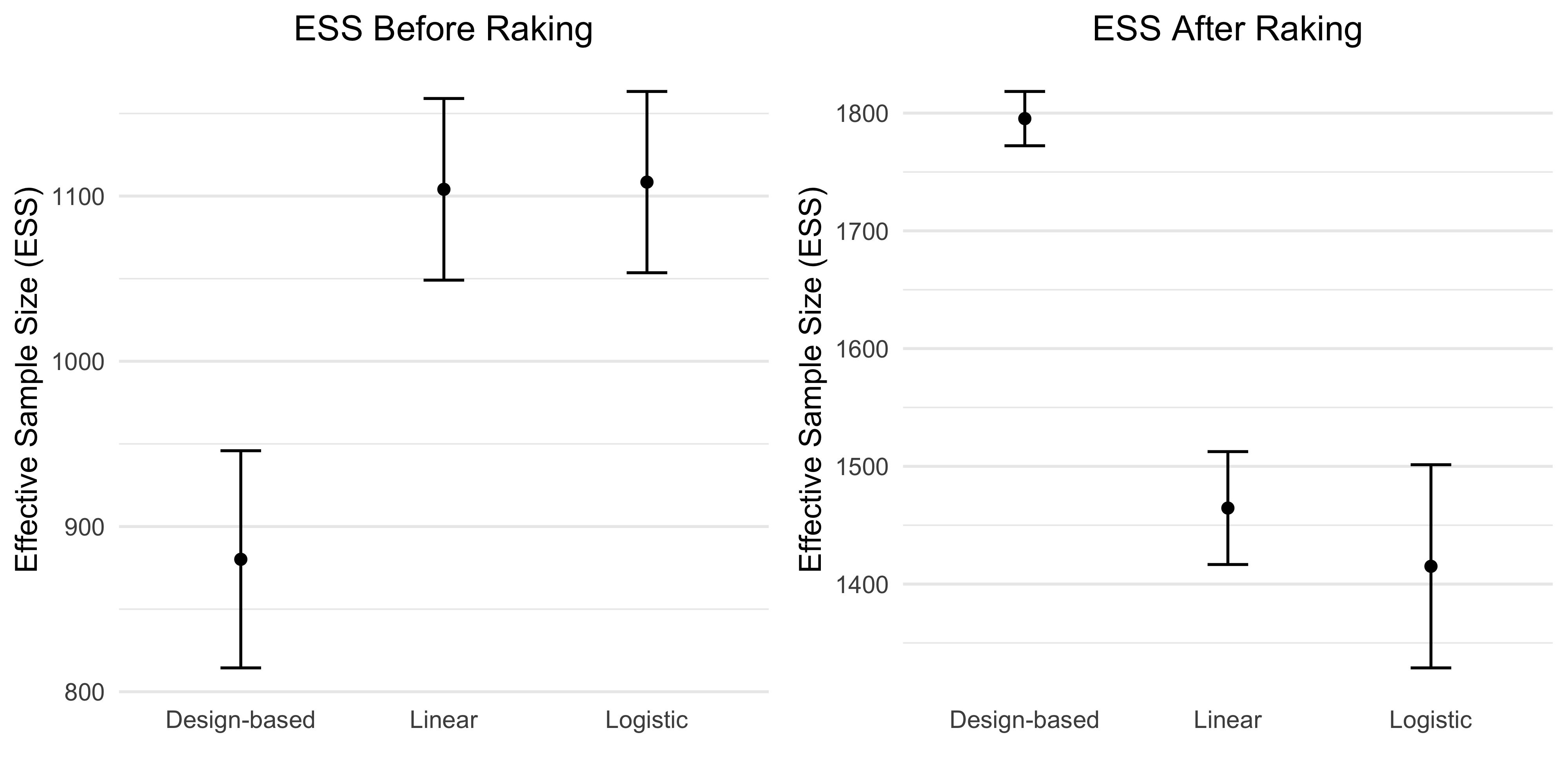
Figure 2(b) presents the effective sample size (ESS) of the three weighting methods across the 300 simulated samples, before and after raking. Before raking, the design-based weights have the lowest ESS, while the linear and logistic equivalent weights have substantially larger and similar ESS values. After raking, the pattern changes: the design-based weights have the highest ESS, whereas the linear and logistic weights have lower ESS, with the logistic weights yielding the lowest ESS among the three methods. Thus, in this simulation, raking increases the ESS of the design-based weights but reduces the ESS of the model-based equivalent weights. These results illustrate that raking can substantially alter the concentration of the weights and that the effect of raking differs across weighting constructions.

Next, we evaluate the finite-sample performance of the three equivalent-weight estimators in estimating the population mean of a binary outcome. The simulation target is the superpopulation mean
where denotes the true outcome probability used to generate the binary responses. Table 1 reports the Monte Carlo mean of the estimator, bias, mean squared error (MSE), and empirical standard deviation.
| Method | Estimate | Bias | MSE | Empirical SD |
|---|---|---|---|---|
| Design-based | 0.352 | -0.021 | 0.000595 | 0.0121 |
| Linear | 0.374 | 0.001 | 0.000148 | 0.0121 |
| Logistic | 0.369 | -0.004 | 0.000194 | 0.0134 |
| Population mean | 0.373 | |||
The linear estimator has the smallest MSE in this simulation and is approximately unbiased, while the logistic estimator also exhibits small finite-sample bias and competitive MSE. The design-based estimator has the largest bias and MSE under the data-generating process considered. These results illustrate that the proposed logistic equivalent weights provide competitive finite-sample point estimation, although they do not uniformly dominate the alternative weighting methods.
Although the overall population mean provides the primary measure of finite-sample performance, it can mask heterogeneity in estimation across population subgroups. We therefore conduct a secondary city-level analysis using the 16 city categories included in the simulation. For city , let
denote the corresponding population prevalence, where is the population size of city . Figure 3 shows the distribution of the estimated city-level prevalence across the 300 simulated samples, with the corresponding population prevalence indicated by the red points.

The city-level results provide a complementary assessment of the overall population-mean results in Table 1. The red points indicate the corresponding population prevalence for each city, allowing the location and dispersion of the sampling distributions to be compared across weighting methods. The raw linear and logistic estimators exhibit greater between-sample variability than the design-based estimator for several cities, with the variability being particularly pronounced for the logistic estimator in some subgroups. At the same time, the centers of the model-based distributions are generally close to the corresponding population prevalences. After raking, the distributions become more concentrated around the city-level population prevalences for most cities, although the magnitude of this change varies across cities and weighting methods.
To further connect the finite-sample evidence with the asymptotic theory, we provide an additional check of Theorem 1. The theorem establishes that the effective sample size ratio satisfies
Under the finite-cell framework, the population limit can be written as
Using 300 simulation replications, we compare the empirical ESS ratio computed from the estimated individual equivalent weights,
with a cell-based finite-sample approximation to the population limit,
The latter uses the population-limit equivalent weights while replacing the population cell proportions by their empirical counterparts . Since , this cell-based quantity converges to the population ESS limit in Theorem 1.
Table 2 reports the mean and interquartile range of the two quantities across the 300 replications. The empirical ESS ratio and the cell-based approximation are similar, providing finite-sample evidence consistent with the convergence established in Theorem 1.
| Mean | IQR [Q1, Q3] | |
|---|---|---|
| Empirical ESS ratio | 0.371 | [0.360, 0.385] |
| Cell-based approximation | 0.379 | [0.369, 0.393] |
Finally, to assess the asymptotic linearity result in Theorem 2, we examine the finite-sample distribution of the centered and scaled equivalent-weight estimator. For each replication, let denote the logistic equivalent-weight estimator and let denote its population-limit target. Theorem 2 establishes that
where
and is the influence function given in Theorem 2.
We therefore assess the corresponding standardized statistic
which should be approximately standard normal in finite samples. A normal Q–Q plot of is used to assess the adequacy of this asymptotic normal approximation. The Q–Q plot of the standardized estimator shows close agreement with the standard normal distribution over the central portion of the distribution, with modest deviations in the tails. This provides evidence that the normal approximation underlying the Wald inference is reasonable in the simulated setting.

We next evaluate the plug-in variance estimator from Theorem 2. For asymptotic variance estimation, we use the unnormalized raw equivalent weights when computing the gradient term , while the equivalent weights are normalized to sum to n in the weighted-mean component of the influence function. This normalization ensures that is expressed on the scale required in Theorem 2. Across the 300 replications, the estimated asymptotic variance has mean approximately and interquartile range approximately . The empirical Monte Carlo asymptotic variance is approximately , indicating close agreement between the plug-in variance estimator and the observed sampling variability.
For comparison, we also construct Wald confidence intervals for the linear equivalent-weight estimator using its standard influence-function variance estimator. For the linear equivalent-weight estimator, we estimate its asymptotic variance using the corresponding influence function. Let denote the OLS coefficient estimator, , and let denote the population mean of the design variables. The estimated influence function for observation is
giving the plug-in estimator of the asymptotic variance
Table 3 reports the empirical Monte Carlo variance, mean estimated variance, mean standard error, and empirical coverage of nominal confidence intervals.
| Method | Empirical | Mean | Mean SE | 95% Coverage |
|---|---|---|---|---|
| Linear | 0.437 | 0.479 | 0.0126 | 97.6% |
| Logistic | 0.542 | 0.562 | 0.0136 | 94.7% |
For the logistic estimator, the mean plug-in variance estimate () is close to the empirical Monte Carlo variance (). The resulting nominal Wald confidence intervals achieve empirical coverage, indicating approximately nominal finite-sample inference in this simulation. The linear estimator also shows good coverage at , although its plug-in variance estimate is somewhat more conservative in this setting.
4.2 Applications to FFCWS Study
We apply the weighting methods to the FFCWS using sampled units representing a population of 1,131,308 individuals. The linear and logistic equivalent weights are first constructed in their raw form, without imposing positivity constraints. Because equivalent weights are interpreted as local sensitivity coefficients rather than sampling probabilities, negative values are retained in the raw model-based estimators. For comparisons involving raking, a separate positivity-adjustment step is required because the raking procedure requires positive starting weights. The resulting raked weights are therefore treated as calibrated versions of the raw equivalent weights rather than as the equivalent weights themselves.
The logistic model uses father interview status as the binary response for constructing the weights because this variable has no missing values. This response is used only to construct the weights; the substantive outcome analyzed below is CPS contact. Recent work using the FFCWS has documented underreporting of CPS involvement in self-reported measures and examined its implications for analyses of young-adult outcomes (Berger et al., Berger et al. 2026). We use CPS contact here as the substantive outcome for illustrating the proposed weighting and inference framework. When raking the model-based weights, we use the same four demographic variables as in the national FFCWS weights, excluding city. We refer to the national FFCWS weights as the design-based weights; these weights are already calibrated in the FFCWS data.
The population-count results in Table 4 show that the linear and logistic model-based procedures reproduce the overall population total exactly after normalization, but allocate the total differently across education categories. These differences illustrate how the model-based approaches use the observed relationships between the weighting variables and the model outcome to distribute population mass across poststratification cells, rather than reproducing the national design-based allocation exactly.
Table 5 shows that the raw logistic equivalent weights have the largest ESS among the model-based methods, with an ESS of 1,435 compared with 1,273 for the linear equivalent weights. After raking, the logistic weights likewise have the largest ESS among the raked methods, with an ESS of 1,301 compared with 1,082 for the raked linear weights, while the raked design-based weights have the lowest ESS. Thus, in this application, the logistic construction achieves a relatively large effective sample size both before and after raking.
| Education | 8 grade | Some HS | HS | Some College | College+ | Total |
|---|---|---|---|---|---|---|
| Design-raked | 111,324 | 211,988 | 340,211 | 214,319 | 253,467 | 1,131,309 |
| Linear model | 73,232 | 267,083 | 367,476 | 242,049 | 181,469 | 1,131,309 |
| Logistic model | 60,214 | 207,301 | 316,517 | 258,784 | 288,491 | 1,131,309 |
| Design-based | Linear | Logit | Linear-raked | Logit-raked | |
|---|---|---|---|---|---|
| ESS | 527 | 1273 | 1435 | 1082 | 1301 |
Using the logistic equivalent weights, the estimated prevalence of CPS contact in the FFCWS is with plug-in variance estimate , yielding a 95% confidence interval of under the proposed variance calculation. This illustrates how the proposed variance estimator can be applied to a single survey dataset without bootstrap or replication-based variance estimation. Because the weighting response and substantive outcome are different variables in this application, the estimate should be interpreted primarily as an illustration of the weighting and inference framework rather than as evidence that father interview status is itself an adequate predictive model for CPS-contact prevalence.
To examine subgroup behavior, we compare CPS-contact prevalence across cities in Figure 5. The weighting methods produce different adjustments across cities, with the magnitude of the change depending on the weighting method and the city. The design-based and linear weights produce relatively similar patterns across cities, whereas the logistic weights produce larger adjustments for several cities. Thus, the application illustrates that the choice of weighting method can have heterogeneous effects across population subgroups, even when the overall population estimate is relatively stable.

5 Discussion
5.1 Key Findings
This study develops a frequentist equivalent-weight construction for logistic regression under categorical poststratification. The central contribution is to represent the nonlinear model-based population estimator locally through weights defined as scaled derivatives with respect to the observed outcomes. Specifically, starting from the logistic estimating equations, we use implicit differentiation of the score equation, followed by the chain rule for the model-based population estimator, to obtain
This provides a direct interpretation of the equivalent weights as local sensitivity coefficients and yields a closed-form expression that can be evaluated from the fitted logistic model and the population cell structure.
This frequentist development is closely related to the locally equivalent-weight framework of Giordano et al. (Giordano et al. 2026), whose Bayesian MrP formulation leads to a corresponding closed-form expression under categorical poststratification. The present work focuses instead on the frequentist survey-weighting interpretation and inference, including effective sample size, asymptotic linearity, plug-in variance estimation, and finite-sample evaluation.
The simulation results provide several findings regarding the practical behavior of the proposed construction. First, both linear and logistic model-based weighting achieve lower regression-coefficient MSE than the design-based and unweighted approaches in the simulated setting, although the advantage is not uniform across replications. Thus, incorporating outcome information through a regression model can improve regression performance under the data-generating process considered.
For overall population-mean estimation, the linear equivalent-weight estimator performs best in the reported simulation, with an MSE of and essentially no bias. The logistic estimator has a slightly larger MSE of and a small bias of , but remains competitive with the linear estimator. These results do not support a claim that logistic equivalent weighting uniformly improves point estimation. Rather, they demonstrate that the nonlinear logistic construction can provide population estimates comparable to established weighting approaches while allowing a nonlinear outcome model to be incorporated into the equivalent-weight framework.
A second useful property of the proposed construction is that the resulting weights can be examined using effective sample size. In the simulation, the model-based equivalent weights, particularly the logistic weights, show relatively stable ESS performance before and after raking. Before raking, the logistic weights have the largest ESS, although their ESS is very close to that of the linear equivalent weights. After raking, the linear and logistic weights remain similar in ESS, with the linear weights yielding a slightly larger ESS in this simulation. The cell-based and empirical ESS ratios are also close to one another, providing finite-sample evidence consistent with the population ESS limit established theoretically. For the simulated sample size of , the empirical ESS ratio of approximately corresponds to an effective sample size of approximately .
The simulation also provides evidence supporting the proposed frequentist inference. The logistic estimator has an empirical Monte Carlo variance of compared with a mean plug-in variance estimate of . The resulting Wald confidence intervals achieve empirical coverage for a nominal confidence level. Together with the approximately Gaussian behavior of the centered and scaled estimator, these results suggest that the asymptotic linear representation and plug-in variance estimator provide a useful finite-sample approximation at the sample size considered.
The city-level analysis provides an important complement to the overall population-mean comparison. Although the linear estimator has the smallest overall MSE in the simulation, the city-level results suggest that model-based weighting can provide useful local population recovery across heterogeneous subgroups. The logistic estimator often places the center of the city-level sampling distribution close to the corresponding population prevalence, but this improvement in local recovery can be accompanied by greater between-sample variability in some cities. This suggests a local bias–variance tradeoff: the flexibility of the nonlinear logistic model can improve recovery for particular subgroups, while the resulting equivalent weights may also be more sensitive to the realized sample composition within those subgroups. Raking generally reduces this variability and brings the city-level estimates into closer alignment with their population benchmarks.
5.2 Limitations
Several limitations should be emphasized. First, the proposed logistic equivalent weights provide a local representation of a nonlinear model-based population estimator rather than an exact global representation by a fixed weighted sample mean. The weights therefore describe first-order sensitivity at the observed data and may not characterize the behavior of the estimator under large changes in the outcomes. The local nature of the representation is intrinsic to the nonlinear logistic model rather than a consequence of an estimation approximation that can simply be removed.
Second, the equivalent weights can be negative or highly variable. Negative values are mathematically permissible because the weights are local sensitivity coefficients rather than sampling probabilities. However, such weights can complicate their use in procedures designed for conventional positive survey weights, including some calibration and raking procedures. In particular, positivity constraints may require a separate calibration or transformation step if the equivalent weights are to be used as starting weights for such procedures. Any such transformation defines a different estimator and is not covered by the theoretical results developed here. The present theory therefore concerns the raw equivalent weights and should not be interpreted as providing inference for arbitrary positivity-constrained or calibrated versions.
Third, the validity of the logistic construction depends on the specification of the outcome model and on the choice of weighting variables. The simulations considered here do not provide a comprehensive assessment of model misspecification, omitted interactions, nonlinear effects, or sparse poststratification cells. In settings where the logistic model poorly describes the relationship between the outcome and the weighting variables, the resulting population estimator and its equivalent weights may perform differently from the results reported here. A systematic comparison under model misspecification is therefore an important direction for future work.
Fourth, the asymptotic theory is developed under a finite-cell superpopulation framework rather than a general design-based theory for complex surveys. In particular, the current results do not explicitly account for clustering, unequal-probability multistage sampling, or design effects arising from complex sample designs. Extending the theoretical results to these settings would broaden the applicability of the proposed construction.
Fifth, the method requires population information for the poststratification cells. The quality of the resulting population estimator therefore depends on the availability and accuracy of the population cell counts and on the choice of auxiliary variables. The method does not automatically incorporate auxiliary information that is not represented in the specified poststratification structure.
Finally, the FFCWS application should be interpreted primarily as an illustration of the weighting and variance-estimation framework. The logistic weights are constructed using father interview status, whereas the substantive outcome is CPS contact. Consequently, the application does not by itself establish that the weighting model is optimal for estimating CPS-contact prevalence. Rather, it demonstrates how the proposed equivalent weights and plug-in variance estimator can be implemented in an empirical survey setting.
5.3 Future Research
Several extensions are natural. First, the theoretical results could be generalized to complex survey designs, including stratified multistage sampling, clustering, and unequal-probability sampling. Second, a systematic study of model misspecification could clarify when logistic weighting provides an advantage over linear or design-based approaches. Third, methods for stabilizing extreme and negative weights could be developed with explicit calibration and inferential guarantees.
A further direction is to incorporate richer population information through hierarchical and nonparametric models. In particular, Gaussian-process and hierarchical Bayesian approaches can provide flexible representations of population-level relationships while allowing uncertainty about sparse cells to be propagated through the weighting procedure. Such extensions provide a natural direction for future work.
Appendix A Supplementary One-Unit Perturbation Analysis
This appendix provides a supplementary numerical assessment of the sensitivity of the logistic equivalent weights to individual outcome perturbations. This analysis is not required for the derivation of the equivalent weights in Section 2 or for the asymptotic results. Instead, it examines the extent to which the fitted weights may change when a single observed binary outcome is perturbed.
A.1 One-Unit Perturbation Analysis
Let denote the response vector obtained by changing an observed value to , while leaving all other outcomes unchanged. Equivalently,
where has its in position .
For each perturbation, the logistic regression model is re-estimated using , and the equivalent weights are recomputed. Denote the resulting weight vector by
while denotes the weights obtained from the original observed response vector.
A first-order finite-difference approximation to the derivative of the weight vector with respect to is
| (30) |
because . Thus, the change in the fitted weight vector resulting from changing one observed outcome from to provides a direct numerical approximation to its local outcome sensitivity.
Because is binary, the Jacobian–vector product can be written as
Using the one-unit perturbations in (30) gives the finite-difference approximation
| (31) |
This calculation provides a direct numerical assessment of the magnitude of the outcome-dependent component of the fitted weights.
A.2 Empirical Sensitivity Assessment
Across the simulation experiments, the outcome-dependent correction term was extremely small. The observed values ranged from approximately to , with mean approximately and median approximately .
In a separate one-unit perturbation check, changing a single binary outcome altered
by at most approximately , with a median change of approximately .
These calculations provide a numerical sensitivity check for the settings considered. They suggest that the indirect dependence of the fitted equivalent weights on individual outcomes through the fitted logistic model is small in the simulation and empirical settings examined. They are not intended to establish that outcome dependence is asymptotically negligible under all sampling designs or model configurations, and they are not required for the derivation of the equivalent weights.
Appendix B Proofs
B.1 Proof of Lemma 1
Proof.
Recall that
where
and
Because the number of poststratification cells is finite and is finite, there exists a finite constant such that
Moreover,
Since and are fixed neighborhoods and the cell vectors and target proportions are fixed, the vector is uniformly bounded on . Thus, for some finite constant ,
By assumption,
for every . Since is symmetric positive definite,
Consequently,
Hence there exists such that
This proves the uniform envelope.
For continuity, the logistic function is continuously differentiable, and hence is continuous in . Therefore and are continuous in . Since remains uniformly nonsingular on , the matrix inverse is continuous. It follows that
is continuous for every .
Finally, since
for every , and there are finitely many cells,
Thus the empirical weights satisfy the stated envelope uniformly in .
∎
B.2 Proof of Theorem 1
Proof.
For notational simplicity, write
It follows that
By the ordinary law of large numbers,
Therefore,
The same argument applies to the squared weights. By the uniform envelope in Lemma 1, the squared weights are uniformly bounded, so
Consequently,
converges by the continuous mapping theorem to
∎
B.3 Proof of Lemma 2
Proof.
For notational simplicity, write
The logistic variance function
is continuously differentiable. Its gradient is
Since is finite and , these derivatives are uniformly bounded on .
Therefore and are continuously differentiable in .
Because is uniformly nonsingular, the matrix inverse is continuously differentiable, with derivative
For a direction in ,
and
Because there are finitely many cells and all cell vectors and probabilities are bounded, there exists a finite constant such that
Similarly, because is linear in , for a direction ,
while does not depend on . Hence
Again, finite-dimensionality, bounded cell vectors, and the uniform bound on imply that there exists a finite constant such that
Thus the population-limit raw equivalent weight is continuously differentiable in both and .
Finally, define
The denominator is bounded away from zero in a sufficiently small neighborhood of because the limiting equivalent weights have a nonzero population mean. Therefore the quotient rule implies that is continuously differentiable in both arguments.
∎
B.4 Proof of Theorem 2
Proof.
For clarity, write
and define
By definition,
Also define, for fixed ,
Thus
The sample estimator can be written as
We first separate the ordinary empirical-process contribution from the plug-in contribution:
| (32) |
where is the empirical-process remainder caused by replacing with inside the empirical weighted mean.
Step 1: Direct sampling variation.
Consider the first term in (32). Since
and
the law of large numbers and the central limit theorem give
Thus the direct sampling contribution to the influence function is
Step 2: Effect of estimating .
By Lemma 2, is continuously differentiable. Define
A first-order Taylor expansion gives
because the logistic MLE satisfies
Under the stated logistic regularity conditions,
Therefore,
Step 3: Effect of estimating the cell probabilities.
The finite-sample weights depend on the empirical cell proportions
Define the cell-indicator vector
Then
and hence
Define
A first-order Taylor expansion gives
Consequently,
Step 4: Empirical-process remainder.
It remains to show that replacing by inside the empirical weighted mean does not produce an additional first-order term.
By Lemma 2, the map is uniformly Lipschitz on the finite-dimensional compact parameter space . Hence is a finite-dimensional parametric class with a bounded envelope and is -Donsker.
Since
stochastic equicontinuity gives
The same argument applies to the denominator. Thus
Step 5: Combine the contributions.
Combining Steps 1–4 yields
where
Each term has finite second moment under the stated assumptions. Therefore, by the multivariate central limit theorem,
where
Finally, the plug-in estimators , , , and the normalized equivalent weights are consistent by the preceding regularity results and the law of large numbers. Hence the estimated influence contributions converge in to , and therefore
∎
Appendix C Data and Code Availability
Selected R code used to reproduce the simulations and empirical analyses in this paper is publicly available at https://github.com/huneel777/logit_equivalent_weight.
The empirical application uses data from the Future of Families and Child Wellbeing Study (FFCWS). Public-use data and documentation are available at https://ffcws.princeton.edu/documentation.
References
- Bethlehem, Cobben and Schouten (2011) Bethlehem, J., Cobben, F. and Schouten, B. (2011). Handbook of Nonresponse in Household Surveys. Wiley, Hoboken.
- Berger et al. (2026) Berger, L. M., Dickerson, T. M., Gelman, A., Jung, H.-M., Lee, S., Thomas, M. M. C. and Waldfogel, J. (2026). Adjusting for Underreporting of Child Protective Services Involvement in the Future of Families and Child Wellbeing Study and Assessing Its Empirical Implications Through Illustrative Analyses of Young Adult Disconnection. Social Service Review 100(1), 69–121. doi:10.1086/739357.
- Carlson (2008) Carlson, B. L. (2008). Fragile Families & Child Wellbeing Study: Methodology for Constructing Mother, Father, and Couple Weights for Core Telephone Public Survey Data Waves 1–4. Future of Families and Child Wellbeing Study, Princeton University.
- Chapman, Bailey and Kasprzyk (1986) Chapman, D. W., Bailey, L. and Kasprzyk, D. (1986). Nonresponse adjustment procedures at the U.S. Bureau of the Census. Survey Methodology 12, 161–180.
- Chen et al. (2017) Chen, Q., Elliott, M. R., Haziza, D., Yang, Y., Ghosh, M., Little, R. J. A., Sedransk, J. and Thompson, M. (2017). Approaches to improving survey-weighted estimates. Statistical Science 32(2), 227–248.
- Chu and Goldman (1997) Chu, A. and Goldman, J. (1997). Weighting procedures for USDA’s Continuing Survey of Food Intakes by Individuals (1994–96). In Proceedings of the Section on Survey Research Methods, American Statistical Association, 802–807.
- Deville and Särndal (1992) Deville, J.-C. and Särndal, C.-E. (1992). Calibration estimators in survey sampling. Journal of the American Statistical Association 87(418), 376–382.
- Gelman (2007) Gelman, A. (2007). Struggles with survey weighting and regression modeling. Statistical Science 22(2), 153–164.
- Giordano et al. (2026) Giordano, R., Cima, A., Murray, J., Hartman, E. and Feller, A. (2026). Locally equivalent weights for multilevel regression and poststratification. arXiv preprint arXiv:2606.04250.
- Hájek (1971) Hájek, J. (1971). Comment on “An essay on the logical foundations of survey sampling” by D. Basu. In V. P. Godambe and D. A. Sprott (eds.), Foundations of Statistical Inference, 236–242. Toronto: Holt, Rinehart and Winston.
- Hampel et al. (1986) Hampel, F. R., Ronchetti, E. M., Rousseeuw, P. J. and Stahel, W. A. (1986). Robust Statistics: The Approach Based on Influence Functions. Wiley, New York.
- Haziza and Beaumont (2017) Haziza, D. and Beaumont, J.-F. (2017). Construction of weights in surveys: A review. Statistical Science 32(2), 206–220.
- Horvitz and Thompson (1952) Horvitz, D. G. and Thompson, D. J. (1952). A generalization of sampling without replacement from a finite universe. Journal of the American Statistical Association 47(260), 663–685.
- Lee and Gelman (2024) Lee, S. and Gelman, A. (2024). Year 22 Future of Families survey weight adjustment. Future of Families and Child Wellbeing Study, Princeton University.
- Little (1986) Little, R. J. A. (1986). Survey nonresponse adjustments for estimates of means. International Statistical Review 54(2), 139–157.
- Little and Rubin (1987) Little, R. J. A. and Rubin, D. B. (1987). Statistical Analysis with Missing Data. Wiley, New York.
- Liu and Fan (2023) Liu, Y. and Fan, Y. (2023). Biased-sample empirical likelihood weighting for missing data problems: An alternative to inverse probability weighting. Journal of the Royal Statistical Society: Series B 85(1), 67–83.
- Lu and Gelman (2003) Lu, H. and Gelman, A. (2003). A method for estimating design-based sampling variances for surveys with weighting, poststratification, and raking. Journal of Official Statistics 19, 133–151.
- Rao and Molina (2015) Rao, J. N. K. and Molina, I. (2015). Small Area Estimation, 2nd ed. Wiley, Hoboken.
- Reichman et al. (2001) Reichman, N. E., Teitler, J. O., Garfinkel, I. and McLanahan, S. S. (2001). Fragile Families: Sample and design. Children and Youth Services Review 23(4–5), 303–326.
- Skinner and Wakefield (2017) Skinner, C. J. and Wakefield, J. (2017). Introduction to the design and analysis of complex survey data. Statistical Science 32(2), 165–175.
- Valliant, Dever and Kreuter (2013) Valliant, R., Dever, J. A. and Kreuter, F. (2013). Practical Tools for Designing and Weighting Survey Samples. Chapman & Hall/CRC, Boca Raton.
- Valliant and Dever (2018) Valliant, R. and Dever, J. A. (2018). Survey Weights: A Step-by-Step Guide to Calculation. Stata Press, College Station.
- van der Vaart (1998) van der Vaart, A. W. (1998). Asymptotic Statistics. Springer, New York.
- Vegetabile, Gillen and Stern (2020) Vegetabile, B. G., Gillen, D. L. and Stern, H. S. (2020). Optimally balanced Gaussian process propensity scores for estimating treatment effects. Journal of the Royal Statistical Society: Series A 183(1), 355–377.
- Wald (1949) Wald, A. (1949). Note on the consistency of the maximum likelihood estimate. Annals of Mathematical Statistics 20(4), 595–604.