Flippered hyperbolic surfaces and renormalized volumes of their moduli spaces I

Yi Huang and Ivan Telpukhovskiy

Date: August 23, 2026

Abstract.

We introduce a natural class of hyperbolic surfaces called flippered surfaces that generalize crowned hyperbolic surfaces (i.e.: worldsheets for open strings). We develop their Teichmüller and moduli-space theory, construct generalized Weil–Petersson volume forms and Chekhov’s action, and prove that the resulting generalized Mirzakhani volumes are finite. We establish three geometric recursion formulae—neck chopping, disk excision, and crown extraction—which express these volumes in terms of those of topologically simpler surfaces. For the fundamental polygonal and annular cases, we derive integral representations involving conical Legendre functions, as well as explicit formulae in terms of elliptic integrals and polylogarithms. We further describe the arithmetic structure of the Taylor coefficients of these volumes, show that suitable specializations are Kontsevich–Zagier periods, and prove identities at the imaginary boundary length $2\pi\sqrt{-1}$ that generalize the Do–Norbury paraphrasing of string and dilaton-type equations.

1. Introduction

Oriented worldsheets of open strings are Riemann surfaces with boundary. In the puncture description of open–closed string theory, open-string insertions are represented by boundary punctures, whereas closed-string insertions are represented by interior punctures. The uniformization (see, e.g., [18, Pg. 24]) of such surfaces are crowned hyperbolic surfaces [5]. The natural generalization of the Weil–Petersson volume form on the moduli spaces of crowned hyperbolic surfaces [6, 14, 17] has infinite volume, and Chekhov [6] suggested a renormalization via an action functional $S\colon\mathcal{M}_{\Sigma}(\vec{b})\to\mathbb{R}_{+}$ on the moduli space of crowned hyperbolic surfaces and defined Mirzakhani volumes as the integrals

V_{\Sigma}(\vec{b})=\int_{\mathcal{M}_{\Sigma}(\vec{b})}e^{-S(X)}\,\Omega^{\text{WP}}_{\Sigma}(\vec{b}).

In [17], we showed that $V_{\Sigma}(\vec{b})$ lies in $\mathbb{Q}_{>0}\!\left[b_{1}^{2},\ldots,b_{m}^{2},\,\log 2,\,\zeta(j),\,\beta(k)\right]$ , where the constants are integer-evaluated values of the Riemann zeta function and Dirichlet beta function.

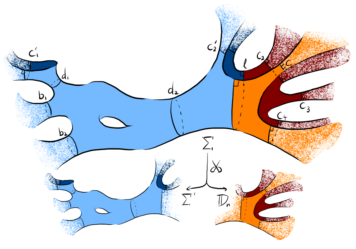
In this paper, we replace point-like punctures by slits of positive size. We refer to the hyperbolic uniformizations of such Riemann surfaces as flippered hyperbolic surfaces (see Definition 2.5). Roughly speaking, just as uniformization geometrizes interior and boundary punctures respectively as cusps and half-cusps (a.k.a. tines), uniformization geometrizes interior and boundary (removed) intervals as funnels and half-funnels (a.k.a. flippers). See Fig. 1 for an example.

Our goal is to define and develop the Weil–Petersson/Mirzakhani volume theory of moduli spaces of flippered hyperbolic surfaces. In particular, we shall see that their moduli spaces naturally arise in various topologically flavored volume recursion formulae in the volumes for crowned hyperbolic surfaces.

We make special mention of [14], where Goncharov and Sun study the volumes of certain slices of the decorated moduli space of crowned hyperbolic surfaces and integrate via normalization with respect to a potential based on horocycle lengths (albeit phrased in terms of areas in their paper). There are strong structural similarities between our works which should be the subject of future investigation.

Refer to caption — Figure 1. A flippered hyperbolic surface with *cuffs* of lengths $\vec{b}=(b_{1},b_{2},0)$ , *straps* of lengths $\vec{c}=(c_{1},\ldots,c_{5},0,c_{7})$ and *necks* of lengths $\vec{d}=(d_{1},d_{2},d_{3})$ .

1.1. Teichmüller and moduli space theory of flippered surfaces

In Sections 2, 3 and 4, we develop the necessary framework for Teichmüller and moduli space theory of flippered hyperbolic surfaces:

•

$\Sigma=\Sigma_{g,m,\vec{a}}$ , where $\vec{a}=(a_{1},\ldots,a_{l})$ , is an oriented surface with genus $g$ , $m$ cuffs, and $l$ crowns respectively with $a_{1},\ldots,a_{l}$ boundary punctures (yielding a total of $n=a_{1}+\ldots+a_{l}$ boundary punctures);
•

the Teichmüller space $\mathcal{T}_{g,m,\vec{a}}=\mathcal{T}_{\Sigma}$ is the space of isotopy classes of flippered hyperbolic metrics on $\Sigma$ ;
•

the moduli space $\mathcal{M}_{g,m,\vec{a}}=\mathcal{M}_{\Sigma}$ is $\mathcal{T}_{\Sigma}/\text{MCG}_{\Sigma}$ ;
•

$\mathcal{M}_{\Sigma}(\vec{b};\vec{c})$ is the subset of $\mathcal{M}_{\Sigma}$ consisting of surfaces with fixed cuff lengths $\vec{b}=(b_{1},\ldots,b_{m})\in[0,\infty)^{m}$ and $n$ straps of fixed lengths $\vec{c}=(\vec{c}_{1},\ldots,\vec{c}_{l})=(c^{(1)}_{1},\ldots,c^{(a_{1})}_{1},\ldots,c^{(1)}_{l},\ldots,c^{(a_{l})}_{l})\in[0,\infty)^{n}$ ;
•

$\mathcal{M}_{\Sigma}(\vec{b};\vec{c}\;|\vec{d})$ is the subset of $\mathcal{M}_{\Sigma}(\vec{b};\vec{c})$ consisting of surfaces with necks of length $\vec{d}=(d_{1},\ldots,d_{k})\in(0,\infty)^{l}$ ;
•

generalised Weil–Petersson volume forms $\Omega^{\text{WP}}_{\Sigma}(\vec{b};\vec{c})$ and $\Omega^{\text{WP}}_{\Sigma}(\vec{b};\vec{c}\;|\vec{d})$ on the respective moduli spaces $\mathcal{M}_{\Sigma}(\vec{b};\vec{c})$ and $\mathcal{M}_{\Sigma}(\vec{b};\vec{c}\;|\vec{d})$ (see Definition 4.6);
•

generalised Chekhov’s function $S\colon\mathcal{M}_{\Sigma}(\vec{b};\vec{c})\to\mathbb{R}_{+}$ (see Definition 3.8).

There are important differences between the Teichmüller theory of flippered surfaces and what is available via established cluster algebraic theory: we are unaware of a natural candidate for a “Weil–Petersson” Poisson algebraic structure.

Definition 1.1 (Generalised Mirzakhani volume).

We refer to

(1)		$\displaystyle V_{\Sigma}(\vec{b};\vec{c}\;\|\vec{d})$	$\displaystyle=\int_{\mathcal{M}_{\Sigma}(\vec{b};\vec{c}\;\|\vec{d})}e^{-S(X)}\;\Omega^{\mathrm{WP}}_{\Sigma}(\vec{b};\vec{c}\;\|\vec{d})$
(2)		$\displaystyle V_{\Sigma}(\vec{b};\vec{c})$	$\displaystyle=\int_{\mathcal{M}_{\Sigma}(\vec{b};\vec{c})}e^{-S(X)}\,\Omega^{\text{WP}}_{\Sigma}(\vec{b};\vec{c}).$

respectively as the generalised Mirzakhani volumes of $\mathcal{M}_{\Sigma}(\vec{b};\vec{c})$ and $\mathcal{M}_{\Sigma}(\vec{b};\vec{c}\;|\vec{d})$ .

Theorem 1.2 (volume finiteness, Theorem 5.21).

The generalized Mirzakhani volumes of the moduli spaces of flippered surfaces are finite. Moreover, if $c_{i}\geqslant c_{i}^{\prime}$ , then

(3)		$\displaystyle V_{\Sigma}(\vec{b};c_{1},\dotsc c_{i},\dotsc,c_{n}\|\vec{d})$	$\displaystyle\leqslant V_{\Sigma}(\vec{b};c_{1},\dotsc c_{i}^{\prime},\dotsc,c_{n}\|\vec{d})$
(4)		$\displaystyle V_{\Sigma}(\vec{b};c_{1},\dotsc c_{i},\dotsc,c_{n})$	$\displaystyle\leqslant V_{\Sigma}(\vec{b};c_{1},\dotsc c_{i}^{\prime},\dotsc,c_{n}).$

1.2. Main results

We obtain neck (chopping), disk (excision) and crown (extraction) recursions for Mirzakhani volumes.

Proposition 1.3 (neck recursion, Proposition 5.4 (cf. [6, 14, 17])).

Consider $\Sigma=\Sigma^{\prime}\cup\mathbb{A}_{m}$ (see Fig. 2) with $\vec{c}:=(\vec{c}\,^{\prime},c_{1},\ldots,c_{m})$ and $\vec{d}:=(\vec{d}^{\prime},\ell)$ , then

(5)		$\displaystyle V_{\Sigma}\bigl(\vec{b};\vec{c}\;\|\vec{d}\bigr)$	$\displaystyle=V_{\Sigma^{\prime}}\bigl(\vec{b},\ell;\vec{c}\,^{\prime}\|\vec{d}\,^{\prime}\bigr)\cdot V_{\mathbb{A}_{m}}\bigl(c_{1},\ldots,c_{m}\|\ell\bigr)\cdot\ell\text{, and}$
(6)		$\displaystyle V_{\Sigma}\bigl(\vec{b};\vec{c}\bigr)$	$\displaystyle=\int_{0}^{\infty}V_{\Sigma^{\prime}}\bigl(\vec{b},\ell;\vec{c}\,^{\prime}\bigr)\cdot V_{\mathbb{A}_{m}}\bigl(c_{1},\dots,c_{m}\|\ell\bigr)\,\cdot\ell\;\mathrm{d}\ell.$

To simplify the statement of the neck recursion formula, we have used a mild form of notation abuse: $\Sigma$ is not the union of $\Sigma^{\prime}$ and $\mathbb{A}_{m}$ , but rather one has to truncate funnels from $\Sigma^{\prime}$ and $\mathbb{A}_{m}$ before gluing them to form $\Sigma$ . We will adopt similar notation nomenclature through-out, and a more precise relationship between these surfaces are spelled out in Section 3.2.

Theorem 1.4 (disk recursion, Theorem 5.5).

Now consider $\Sigma=\Sigma^{\prime}\cup\mathbb{D}_{n}$ (see Fig. 3) with $\vec{c}:=(\vec{c}\,^{\prime},c_{1},\ldots,c_{n})$ , then

(7)		$\displaystyle V_{\Sigma}\bigl(\vec{b};\vec{c}\;\|\vec{d}\bigr)$	$\displaystyle=\frac{1}{2}\int_{0}^{\infty}V_{\Sigma^{\prime}}\bigl(\vec{b};\vec{c}\,^{\prime},\ell\|\vec{d}\bigr)\cdot V_{\mathbb{D}_{n+1}}\bigl(c_{1},\ldots,c_{n},\ell\bigr)\,\mathrm{d}\cosh\ell\text{, and }$
(8)		$\displaystyle V_{\Sigma}\bigl(\vec{b};\vec{c}\bigr)$	$\displaystyle=\frac{1}{2}\int_{0}^{\infty}V_{\Sigma^{\prime}}\bigl(\vec{b};\vec{c}\,^{\prime},\ell\bigr)\cdot V_{\mathbb{D}_{n+1}}\bigl(c_{1},\ldots,c_{n},\ell\bigr)\,\mathrm{d}\cosh\ell.$

Theorem 1.5 (crown recursion, Theorem 5.9).

Consider $\Sigma=\mathbb{A}_{n}=\mathbb{A}_{n-m}^{\circ}\cup\mathbb{A}_{m}^{\circ}$ (see Fig. 4) with $\vec{c}:=(\vec{c}\,^{\prime},c_{1},\ldots,c_{m})$ , then

(9)		$\displaystyle V_{\Sigma}\bigl(\vec{c}\;\|d\bigr)$	$\displaystyle=\int_{\mathbb{R}}V_{\mathbb{A}_{n-m}}\bigl(\vec{c}\,^{\prime}\|\;\|d-\ell\|\bigr)\cdot V_{\mathbb{A}_{m}}\bigl(c_{1},\ldots,c_{m}\|\;\|\ell\|\bigr)\;\mathrm{d}\ell\text{, and}$
(10)		$\displaystyle V_{\Sigma}\bigl(\vec{c}\bigr)$	$\displaystyle=2\cdot V_{\mathbb{A}_{n-m}}\bigl(\vec{c}\,^{\prime}\bigr)\cdot V_{\mathbb{A}_{m}}\bigl(c_{1},\ldots,c_{m}\bigr).$

The above recursion formulae assert the importance of the volumes of moduli spaces of topologically simpler surfaces such as $\mathbb{D}_{n}$ and $\mathbb{A}_{n}$ . We show:

Theorem 1.6 (Theorem 5.13, Theorem 5.17).

For $n\geqslant 3$ ,

(11)

{V}_{\mathbb{D}_{n}}(c_{1},\dotsc,c_{n})=\pi^{n-2}\int_{0}^{\infty}\xi\sinh{2\pi\xi}\cdot\prod_{i=1}^{n}\frac{P_{-1/2+\sqrt{-1}\xi}(\cosh c_{i})}{\cosh{\pi\xi}}\,\mathrm{d}\xi.

For $n\geqslant 1$ ,

(12)

V_{\mathbb{A}_{n}}(c_{1},\dotsc,c_{n}|d)=\pi^{n-1}\int_{0}^{\infty}\cos(\omega d)\cdot\prod_{i=1}^{n}\frac{P_{-1/2+\sqrt{-1}\omega}(\cosh c_{i})}{\cosh\pi\omega}\,\mathrm{d}\omega.

Corollary 1.7 (Corollary 5.19).

For $n\geqslant 1$ ,

V_{\mathbb{A}_{n}}(c_{1},\dotsc,c_{n})=2^{n-1}\prod_{i=1}^{n}\frac{K\left(\tanh(c_{i}/2)\right)}{\cosh(c_{i}/2)},

where $K(s):=\int_{0}^{1}\frac{\mathrm{d}t}{\sqrt{(1-t^{2})(1-s^{2}t^{2})}}$ is the complete elliptic integral of the first kind.

Theorem 1.8 (Theorem 6.4).

For any $\Sigma$ , the Taylor germ of $V_{\Sigma}(\vec{b};\vec{c})$ in $c$ -variables has coefficients in

\mathbb{Q}[b_{1}^{2},\dotsc,b_{m}^{2},\log 2,\zeta(r),\beta(r)],\quad 1\leqslant r\leqslant\dim_{\mathbb{R}}\mathcal{M}_{\Sigma}(\vec{b};\vec{c}).

Remark 1.9.

Mirzakhani volume integrals are periods in the sense of Kontsevich–Zagier [20] for specialized values of $b_{i}$ and $c_{j}$ (e.g.: when $b_{i}$ and $\cosh c_{j}$ algebraic numbers, see Theorem 6.7). Compare this to the exponential volumes in [14], which are exponential periods [20, §4.3].

Theorem 1.10 (string and dilaton-type equations, Theorem 6.2).

For $\Sigma=\Sigma_{g,m+1,\vec{a}}$ with $2g-2+m+l>0$ , and $\vec{b}=(b_{1},\dotsc,b_{m})$ ,

(13)

\begin{split}V_{\Sigma}(\vec{b},2\pi\sqrt{-1};\vec{c}\;|\vec{d})=&\sum_{i=1}^{m}\int_{0}^{b_{i}}b_{i}V_{\Sigma\cup p_{m+1}}(\vec{b};\vec{c}\;|\vec{d})\,\mathrm{d}b_{i}\\ &+\sum_{j=1}^{l}d_{j}V_{\mathbb{A}_{a_{j}}}(\vec{c}_{j}|d_{j})\int_{0}^{d_{j}}\frac{V_{\Sigma\cup p_{m+1}}(\vec{b};\vec{c}\;|\vec{d})}{V_{\mathbb{A}_{a_{j}}}(\vec{c}_{j}|d_{j})}\mathrm{d}d_{j}.\end{split}

For $\Sigma=\mathbb{A}_{n}$ with $n\geqslant 3$ ,

(14)

\frac{\partial V_{\Sigma}}{\partial d}\left(\vec{c}\;|2\pi\sqrt{-1}\right)=-\pi\sqrt{-1}V_{\Sigma\cup p_{1}}(\vec{c}).

For $\Sigma=\Sigma_{g,m+1,\vec{a}}\neq\mathbb{A}_{n}$ and $\vec{b}=(b_{1},\dotsc,b_{m})$ ,

(15)		$\displaystyle\frac{\partial V_{\Sigma}}{\partial b_{m+1}}\bigl(\vec{b},2\pi\sqrt{-1};\vec{c}\;\|\vec{d}\bigr)$	$\displaystyle=2\pi\sqrt{-1}(2g-2+m+l)V_{\Sigma\cup p_{m+1}}\bigl(\vec{b};\vec{c}\;\|\vec{d}\bigr)\text{, and}$
(16)		$\displaystyle\frac{\partial V_{\Sigma}}{\partial b_{m+1}}\bigl(\vec{b},2\pi\sqrt{-1};\vec{c}\bigr)$	$\displaystyle=2\pi\sqrt{-1}(2g-2+m+l)V_{\Sigma\cup p_{m+1}}\bigl(\vec{b};\vec{c}\bigr).$

Remark 1.11.

These identities generalize the identities given in [8, Theorem 2] which Do and Norbury show generalize the string and dilaton equations (due to Witten [35]).

We conclude this subsection of the introduction by listing some explicit volumes of moduli spaces of flippered surfaces (Theorem 5.1, Theorem 5.2, Theorem 7.1, Theorem 7.2, Proposition 7.4, Proposition 7.6, Proposition 7.8):

$\Sigma$	Generalised Mirzakhani Volume
$\mathbb{D}_{3}$	$V_{\Sigma}(c_{1},c_{2},c_{3})=\frac{2}{\sqrt{\cosh^{2}c_{1}+\cosh^{2}c_{2}+\cosh^{2}c_{3}+2\cosh c_{1}\cosh c_{2}\cosh c_{3}-1}}$
$\mathbb{D}_{4}$	${V}_{\Sigma}(c,c,0,0)=\frac{2}{1+\cosh c}$
$\mathbb{D}_{4}$	$V_{\Sigma}(c_{1},c_{2},0,0)=\frac{2\log\left(\frac{1+\cosh c_{1}}{1+\cosh c_{2}}\right)}{\cosh c_{1}-\cosh c_{2}}$ , if $c_{1}\neq c_{2}$
$\mathbb{D}_{4}$	$V_{\Sigma}(c_{1},c_{2},c_{1},c_{2})=\frac{\log\left(\frac{1+\cosh(c_{1}+c_{2})}{1+\cosh(c_{1}-c_{2})}\right)}{\sinh c_{1}\sinh c_{2}}$
$\mathbb{D}_{5}$	${V}_{\Sigma}(c_{1},c_{2},0,0,0)=\frac{2\mathrm{Li}_{2}(1)+\log^{2}\frac{\cosh c_{1}+1}{\cosh c_{2}+1}+2\sum_{i=1,2}\mathrm{Li}_{2}\left(\frac{\cosh c_{i}-1}{\cosh c_{i}+1}\right)}{\cosh c_{1}+\cosh c_{2}}$
$\mathbb{A}_{1}$	$V_{\Sigma}(c\|d)=\frac{1}{\sqrt{2\cosh c+2\cosh d}}$
$\mathbb{A}_{2}$	$V_{\Sigma}(c,0\|d)=\sqrt{\frac{2}{\cosh c-\cosh d}}\text{arccot}\sqrt{\frac{1+\cosh d}{\cosh c-\cosh d}}$ , if $c>d$
$\mathbb{A}_{2}$	$V_{\Sigma}(c,0\|d)=\frac{1}{\cosh c/2}$ , if $c=d$
$\mathbb{A}_{2}$	$V_{\Sigma}(c,0\|d)=\sqrt{\frac{2}{\cosh d-\cosh c}}\text{arccoth}\sqrt{\frac{\cosh d+1}{\cosh d-\cosh c}}$ , if $c<d$
$\mathbb{A}_{3}$	$V_{\Sigma}(c,\vec{0}\|d)=\frac{2\text{Li}_{2}(1)+\frac{1}{2}\sum\log^{2}\left(\frac{\sqrt{\text{ch}c+\text{ch}d}+\sqrt{\text{ch}d+1}}{\sqrt{\text{ch}c+\text{ch}d}\pm\sqrt{\text{ch}d-1}}\right)+\sum_{1,\dotsc,4}\text{Li}_{2}\left(\frac{\sqrt{\text{ch}c+\text{ch}d}\pm\sqrt{\text{ch}d\pm 1}}{\sqrt{\text{ch}c+\text{ch}d}\pm\sqrt{\text{ch}d\pm 1}}\right)}{\sqrt{2(\text{ch}c+\text{ch}d)}}$
$\mathbb{A}_{1,1}$	$V_{\Sigma}(c,c)=\frac{\mathrm{Li}_{2}(-e^{-c})-\mathrm{Li}_{2}(-e^{c})}{2\sinh c}$

Table 1. Some explicit examples of generalised Mirzakhani volumes.

Explicit expressions do become quite unwieldy quite quickly, see e.g.: formulas for the volumes $V_{\mathbb{D}_{4}}(c_{1},c_{2},c_{3},c_{4})$ and $V_{\mathbb{A}_{2}}(c_{1},c_{2}|d)$ (respectively Theorem 7.2 and Theorem 7.1).

Organisation of the paper

Section 2 sets up the geometry of flippered hyperbolic surfaces: their anatomy, Teichmüller and moduli spaces, and the flipper-clipping and Nielsen cut operations. Section 3 defines the generalised Chekhov action and establishes its recursive properties. Section 4 constructs the Weil–Petersson volume form via flipper-clipping and establishes the Nielsen cut recursion for it. Section 5 proves the finiteness of the renormalised volumes, derives the three volume recursions and computes the volumes of simple surfaces. Section 6 proves the string and dilaton-type equations, determines the structure of the Mirzakhani volume coefficients and establishes that the volumes are periods. Section 7 presents explicit computations of volumes for moduli spaces of some simpler surfaces. Appendix A through Appendix H support us with various facts and somewhat more technical computations used along the way.

AI declaration

Version 5.6 of OpenAI’s ChatGPT was used to explore proof ideas, test preliminary arguments, and identify possible references. The authors independently checked every source and argument, wrote the final text, and assume full responsibility for its content.

Acknowledgements

The authors thank Anton Alekseev, Dylan Allegretti, Norman Do, Maksim Karev, Omar Kidwai, Paul Norbury, Kasra Rafi, and Nicolas Tholozan for useful discussions. The second listed author gratefully acknowledges support from the Beijing Natural Science Foundation (International Scientists Project), Funding No. 1S24065.

2. Teichmüller and Moduli spaces of flippered surfaces

We familiarise ourselves with Teichmüller and moduli spaces of flippered surfaces: in this section we introduce parametrisations of these spaces, to prepare for upcoming volume calculations.

2.1. Worldsheets of open strings as hyperbolic surfaces

Notation 2.1.

For the remainder of the article let $\Sigma:=\Sigma_{g,m,\vec{a}}$ , with $m\in\mathbb{Z}_{\geqslant 0}$ and $\vec{a}=(a_{1},\ldots,a_{l})\in\mathbb{Z}_{>0}^{l}$ , denote a bordered topological surface of finite type (that admits a complete hyperbolic metric) with

•

genus $g$
•

$m$ interior punctures, which we label $\{p_{1},\ldots,p_{m}\}$ ;
•

$n=\sum_{k=1}^{l}a_{k}$ boundary punctures, which we label $\{q_{1},\ldots,q_{n}\}$ ;
•

$\Sigma\cup\{q_{1},\ldots,q_{n}\}$ is a surface with (only) interior punctures and $l$ boundary curves, which we label $\{\delta_{1},\ldots,\delta_{l}\}$ , so that the $i$ -th boundary $\delta_{i}$ contains $a_{i}\geqslant 1$ punctures.

Remark 2.2.

The condition that $\Sigma$ admits a hyperbolic metric means:

•

if $g=0$ and $l=0$ , then $m\geqslant 3$ ;
•

if $g=0$ , $l=1$ and $m=0$ , then $n\geqslant 3$ ;
•

if $g=1$ and $l=0$ , then $m\geqslant 1$ ;
•

if $g\geq 2$ , there are no additional constraints on $l,m,n$ .

By (canonically) extending geodesic boundaries with funnels, Mirzakhani’s moduli spaces $\mathcal{M}_{g,m}(b_{1},\ldots,b_{m})$ is may be regarded as the moduli space of funnelled hyperbolic surfaces with fixed boundary holonomy. This perspective, combined with the surface-doubling approach for studying open strings (see, e.g.: [3, 26]), naturally suggests flippered surfaces as an object of study.

Definition 2.3 (Flippered surface).

We refer to $\Sigma$ , equipped with a complete hyperbolic metric $h$ with (necessarily bi-infinite) geodesic boundaries, as a flippered surface. We henceforth use $X=(\Sigma,h)$ to denote a generic flippered surface.

2.2. The anatomy of a flippered surface

Although basic, we take a moment to affirm the uniqueness of geodesic representatives of homotopy classes of paths on hyperbolic surfaces.

Theorem 2.4 (e.g.: [4, Theorems 1.5.2 and 1.5.3], [18, Lemma 2.10]).

Any essential isotopy class $[c]$ of paths on a hyperbolic surface $\Sigma$ contains a unique (up to parametrisation) shortest curve $\gamma$ . Moreover, $\gamma$ is a geodesic, meets $\partial\Sigma$ perpendicularly (if at all), and is simple if and only if $[c]$ is simple.

Definition 2.5 (arches, cuffs, flippers, straps, and tines).

We refer to the bi-infinite geodesic boundaries of $X$ as arches. The following behaviour can hold at the punctures of a flippered surface $X$ :

•

Interior punctures $p_{i}$ are geometrised as flares/funnels or cusps. For flares, $\beta_{i}$ denotes the geodesic representative of a simple loop around $p_{i}$ and we refer to $\beta_{i}$ as the $i$ -th cuff. For cusps, we use $\beta_{i}$ to denote the cusp $p_{i}$ .
•

A boundary puncture $q_{j}$ geometrises to “half” of a flare/funnel or cusp when $X$ is regarded as a subset of the doubled surface $DX$ . For half-flares, the cuff corresponding to $q_{j}$ on $DX$ restricts to an orthogeodesic on $X$ , and we refer to this orthogeodesic half-cuff as the $j$ -th strap $\sigma_{j}$ . We refer to the half-funnel on $X$ bounded by $\sigma_{j}$ as the $j$ -th flipper. For half-cusps —which we call a tine [18], we use $\sigma_{j}$ to formally denote the tine $q_{j}$ .

For the remainder of the article, we use $X$ to denote a (finite type) flippered hyperbolic surface (see Fig. 1), with

•

$\{\beta_{i}\}_{i=1,\ldots,m}$ denoting the cuffs for its funnels (and cusps);
•

$\{\alpha_{j}\}_{j=1,\ldots,n}$ denoting its boundary arches;
•

$\{\sigma_{j}\}_{j=1,\ldots,n}$ denoting its straps (and tines).

To simplify future notation, we label the straps so that $\sigma_{i}$ always joins $\alpha_{i}$ and $\alpha_{i+1}$ , where the labelling index is cyclic with respect to the number of tines on crown containing these arches and straps.

Definition 2.6 (neck).

Each boundary curve $\delta_{i}$ on $X\cup\{q_{1},\ldots,q_{n}\}$ has a unique homotopy representative $\nu_{i}$ which is a simple closed geodesic on $X$ . We refer to $\nu_{i}$ as the $i$ -th neck of $X$ .

Notation 2.7 (disks and annuli).

There are three classes of examples for which the nomenclature and notation in this paper applies awkwardly or with ambiguity:

•

when $\Sigma$ is a disk with $n\geqslant 3$ boundary punctures, with no interior punctures (i.e.: $m=0$ ) and with no necks. We write $\mathbb{D}_{n}$ to denote such $\Sigma$ , and refer to it as an $n$ -gon.
•

when $\Sigma$ is disk with $n\geqslant 1$ boundary punctures and $m=1$ interior puncture, the surface contains a unique simple closed geodesic, and this geodesic serves as both the cuff of the interior puncture (or a cusp in the non-generic case) as well as the neck of the punctured boundary. We use the notation $\mathbb{A}_{n}$ to denote $\Sigma$ , and refer to $\mathbb{A}_{n}$ as an $n$ -tined crown.
•

when $\Sigma$ is a closed annulus with $a_{1}$ punctures on the first boundary and $a_{2}$ boundary punctures on the second boundary, the surface contains no interior punctures (and hence no cuffs). Moreover, the surface supports a unique simple closed geodesic which serves as a neck for both (punctured) boundaries. We use the notation $\mathbb{A}_{a_{1},a_{2}}$ for such $\Sigma$ and refer to it as an $(a_{1},a_{2})$ -annulus.

2.3. Teichmüller and moduli spaces of flippered surfaces

We define the Teichmüller and moduli space for flippered surfaces in the standard manner:

Definition 2.8 (Teichmüller space).

The Teichmüller space $\mathcal{T}_{\Sigma}$ is defined as the space of isotopy classes of flippered hyperbolic metrics on $\Sigma$ .

Proposition 2.9 (Corollary 2.33).

The Teichmüller space for a flippered hyperbolic surface $\mathcal{T}_{\Sigma}$ is naturally stratified into $2^{n+m}$ strata according to the geometric type of its punctures, described in Definition 2.5. Each stratum is a topological ball, and $\mathcal{T}_{\Sigma}$ has the structure of a manifold with corners of dimension $\frac{1}{2}(3|\chi(D\Sigma)|+n)$ , where $D\Sigma$ is the surface obtained by doubling $\Sigma$ along its boundary.

Definition 2.10 (moduli space).

The moduli space $\mathcal{M}_{\Sigma}$ is defined as the space of isometry classes of flippered hyperbolic surfaces.

The (pure) mapping class group $\mathrm{MCG}_{\Sigma}$ , consisting of isotopy classes of puncture-preserving homeomorphisms of $\Sigma$ , again serves as the group of deck transformations relating $\mathcal{T}_{\Sigma}$ and $\mathcal{M}_{\Sigma}$ :

\mathcal{M}_{\Sigma}=\mathcal{T}_{\Sigma}/\mathrm{MCG}_{\Sigma}.

Definition 2.11 (moduli spaces with fixed holonomy).

For $\vec{b}=(b_{1},\ldots,b_{m})\in[0,\infty)^{m}$ and $\vec{c}=(c_{1},\ldots,c_{n})\in[0,\infty)^{n}$ , define

	$\displaystyle\mathcal{T}_{\Sigma}(b_{1},\ldots,b_{m};c_{1},\ldots,c_{n})$	$\displaystyle=:\mathcal{T}_{\Sigma}(\vec{b};\vec{c})\subset\mathcal{T}_{\Sigma}\quad\text{and}$
	$\displaystyle\mathcal{M}_{\Sigma}(b_{1},\ldots,b_{m};c_{1},\ldots,c_{n})$	$\displaystyle=:\mathcal{M}_{\Sigma}(\vec{b};\vec{c})\subset\mathcal{M}_{\Sigma},$

to respectively be the subsets of hyperbolic surfaces in $\mathcal{T}_{\Sigma}$ and $\mathcal{M}_{\Sigma}$ whose

•

$i$ -th cuff $\beta_{i}$ is of length $b_{i}$ for all $i=1,\ldots,m$ , and
•

$j$ -th strap $\sigma_{j}$ is length $c_{j}$ for all $j=1,\ldots,n$ .

Furthermore, given $\vec{d}=(d_{1},\ldots,d_{l})\in[0,\infty)^{l}$ , define

	$\displaystyle\mathcal{T}_{\Sigma}(b_{1},\ldots,b_{m};c_{1},\ldots,c_{n}\|d_{1},\ldots,d_{l})$	$\displaystyle=:\mathcal{T}_{\Sigma}(\vec{b};\vec{c}\;\|\vec{d})\subset\mathcal{T}_{\Sigma}(\vec{b};\vec{c})\quad\text{and}$
	$\displaystyle\mathcal{M}_{\Sigma}(b_{1},\ldots,b_{m};c_{1},\ldots,c_{n}\|d_{1},\ldots,d_{l})$	$\displaystyle=:\mathcal{M}_{\Sigma}(\vec{b};\vec{c}\;\|\vec{d})\subset\mathcal{M}_{\Sigma}(\vec{b};\vec{c}).$

to respectively be the subsets of hyperbolic surfaces whose $k$ -th neck lengths is $d_{k}$ for all $k=1,\ldots,l$ .

Notation 2.12 (fixed holonomy for special surfaces).

When $\Sigma=\mathbb{D}_{n}$ , $\mathbb{A}_{n}$ , or $\mathbb{A}_{a_{1},a_{2}}$ , the above notation for Teichmüller and moduli spaces with fixed holonomy may not make sense due to the absence of cuffs and/or necks. Instead, we write:

•

$\mathcal{T}_{\mathbb{D}_{n}}(\vec{c})$ and $\mathcal{M}_{\mathbb{D}_{n}}(\vec{c})$ ;
•

$\mathcal{T}_{\mathbb{A}_{n}}(\vec{c}\;|\vec{d})$ and $\mathcal{M}_{\mathbb{A}_{n}}(\vec{c}\;|\vec{d})$ ;
•

$\mathcal{T}_{\mathbb{A}_{a_{1},a_{2}}}(\vec{c};d)$ and $\mathcal{M}_{\mathbb{A}_{a_{1},a_{2}}}(\vec{c};\vec{d})$ .

Remark 2.13.

We show in Corollary 2.34 that Teichmüller spaces with fixed holonomy are open balls (of various dimensions, including $0$ ). In particular, $\mathcal{T}_{\Sigma}(\vec{b};\vec{c})$ embeds as a half-dimensional affine subspace in $\mathcal{T}_{D\Sigma}(b_{1},\ldots,b_{m},b_{1},\ldots,b_{m},2c_{1},\ldots,2c_{n})$ , where $D\Sigma$ is the surface obtained from doubling $\Sigma$ along its boundary, and hence has dimension $\frac{1}{2}(3|\chi(D\Sigma)|-2m-n)$ . The fixed neck length subset $\mathcal{T}_{\Sigma}(\vec{b};\vec{c}\;|\vec{d})$ embeds as a $l$ co-dimensional subset of $\mathcal{T}(\vec{b};\vec{c})$ , i.e.:

\dim_{\mathbb{R}}\mathcal{T}_{\Sigma}(\vec{b};\vec{c}\;|\vec{d})=\tfrac{1}{2}(3|\chi(D\Sigma)|-2m-2l-n).

The fact that doubling allows us to embed various Teichmüller spaces of flippered (and crowned) surfaces as canonical real analytic subspaces in Teichmüller spaces of hyperbolic bordered surfaces means:

Proposition 2.14.

The Teichmüller spaces $\mathcal{T}_{\Sigma}$ , $\mathcal{T}_{\Sigma}(\vec{b};\vec{c})$ , $\mathcal{T}_{\Sigma}(\vec{b};\vec{c}\;|\vec{d})$ and their corresponding moduli spaces all inherit natural and canonical real analytic manifold (possibly with corners) structure as subspaces of $\mathcal{T}_{D\Sigma}$

2.4. Puncture-doubling and flipper clipper

We define operations called puncture-doubling and flipper-clipping, which allows us to relate Teichmüller/moduli spaces of flippered and crowned hyperbolic surfaces.

Notation 2.15 (doubling boundary punctures).

We write $\dot{\Sigma}(j_{1},\dots,j_{k})$ to denote the surface obtained from $\Sigma$ by doubling the boundary punctures $q_{j_{1}},\dots,q_{j_{k}}$ as follows: for each $q_{j_{i}}$ , we remove a small open disk from $\Sigma$ bounded by a contractible arc with endpoints at $q_{j_{i}}$ (see Fig. 5). We refer to $\dot{\Sigma}(j_{1},\dots,j_{k})$ as the puncture-double of $\Sigma$ at $q_{j_{1}},\dots,q_{j_{k}}$ .

Definition 2.16 (flipper-clipping).

Given a flippered surface $X\in\mathcal{T}_{\Sigma}$ , we produce a canonical crowned surface $\operatorname{Clip}(X)\in\mathcal{T}_{\dot{\Sigma}(X)}$ , where $\dot{\Sigma}(X)$ is the puncture-double of $\Sigma$ at (and only at) all flippered boundary punctures of $X$ . The surface $\operatorname{Clip}(X)$ is obtained as follows: for every flipper on $X$ , remove the largest (by inclusion) open half-plane contained inside the flipper (see Fig. 6). We refer to $\operatorname{Clip}(X)$ as the flipper-clipping of $X$ .

Remark 2.17.

Flipper-clipping does not affect cusps. In particular, the flipper-clipping of a crowned hyperbolic surface is unchanged.

To remove the dependence on $X$ in the target Teichmüller space in Definition 2.16, we highlight the following subspaces of $\mathcal{T}_{\Sigma}$ :

Definition 2.18 (flipper-based strata in Teichmüller space).

Given a subset $\mathcal{A}\subseteq\{1,\dotsc,n\}$ , let $\mathcal{T}_{\Sigma}^{\mathcal{A}}\subset\mathcal{T}_{\Sigma}$ be the subset of hyperbolic surfaces in $\mathcal{T}_{\Sigma}$ whose $j$ -th strap $\sigma_{j}$ has (strictly) positive length if and only if $j\in\mathcal{A}$ , for all $j=1,\dotsc,n$ .

Remark 2.19.

Observe that $\mathcal{T}_{\Sigma}(\vec{b};\vec{c})\subset\mathcal{T}_{\Sigma}^{\mathcal{A}}$ when $\mathcal{A}$ is the set of indices for which $c_{j}$ is (strictly) positive. Since it is an open subset, it is also a real-analytic manifold (with corners).

Lemma 2.20 (clipping is bijective).

Given a subset $\mathcal{A}\subset\{1,\dotsc,n\}$ , flipper-clipping defines a bijection

\operatorname{Clip}:\mathcal{T}_{\Sigma}^{\mathcal{A}}\to\mathcal{T}_{\dot{\Sigma}(\mathcal{A})}^{\varnothing}.

Proof.

The reverse process of attaching half-planes to specified arches is canonical and gives the inverse map to $\operatorname{Clip}$ . ∎

In fact, it is intuitively clear that $\operatorname{Clip}$ is a real-analytic homeomorphism (see Corollary 2.35 for a proof). Together with the construction in Section 2.5, we obtain a parametrization of $\mathcal{T}_{\Sigma}^{\mathcal{A}}$ by shearing coordinates in Proposition 2.25.

Remark 2.21.

Although we have introduced flipper-clipping as a function $\operatorname{Clip}:\mathcal{T}_{\Sigma}^{\mathcal{A}}\to\mathcal{T}_{\dot{\Sigma}(\mathcal{A})}^{\varnothing}$ , we will abuse notation and use it to also denote maps between

•

Teichmüller spaces with fixed holonomy $\operatorname{Clip}:\mathcal{T}_{\Sigma}(\vec{b};\vec{c})\to\mathcal{T}_{\dot{\Sigma}}(\vec{b};\vec{0})$ ,
•

Teichmüller spaces of fixed neck lengths $\operatorname{Clip}:\mathcal{T}_{\Sigma}(\vec{b};\vec{c}\;|\vec{d})\to\mathcal{T}_{\dot{\Sigma}}(\vec{b};\vec{0}|\vec{d})$ ,
•

moduli spaces $\operatorname{Clip}:\mathcal{M}_{\Sigma}(\vec{b};\vec{c})\to\mathcal{M}_{\dot{\Sigma}}(\vec{b};\vec{0})$ , and
•

moduli spaces of fixed neck lengths $\operatorname{Clip}:\mathcal{M}_{\Sigma}(\vec{b};\vec{c}\;|\vec{d})\to\mathcal{M}_{\dot{\Sigma}}(\vec{b};\vec{0}|\vec{d})$ .

2.5. Shearing coordinates on Teichmüller space of crowned surfaces

The contents of this subsection is well-known to experts. See, for example, [23, Section 7.4] for a definition of the shearing parameter between two adjacent ideal hyperbolic triangles and the construction of shearing coordinates on Teichmüller space of surfaces with punctures.

Notation 2.22 (shearing sign convention).

We take left shears to be positive.

Definition 2.23 (ideal arcs and ideal triangulation).

Given a surface $\Sigma=\Sigma_{g,m,\vec{a}}$ , we refer to an embedded open arc in $\Sigma$ with “endpoints” placed at the interior and boundary punctures of $\Sigma$ as an ideal arc if it does not bound an open disk in $\Sigma$ . We call a collection $\triangle$ of pairwise disjoint ideal arcs in $\Sigma$ as an ideal triangulation of $\Sigma$ if

•

no arc is peripheral in the sense of being isotopic to one of the arches,
•

no two arcs in $\triangle$ are isotopic via isotopy fixing the endpoints, and
•

$\triangle$ is maximal in cardinality among sets satisfying above conditions.

We identify ideal triangulations up to isotopies of $\Sigma$ .

Lemma 2.24 ([17, Lemma 2.13]).

Given a surface $\Sigma=\Sigma_{g,m,\vec{a}}$ , with $m$ interior punctures and $l$ boundary curves with $n=\sum_{k=1}^{l}a_{k}$ boundary punctures so that there are $a_{k}$ punctures on the $k$ -th boundary (see 2.1), every ideal triangulation $\triangle$ of $\Sigma$ has cardinality

|\triangle|=\tfrac{1}{2}(3|\chi(D\Sigma)|-n),

where $D\Sigma$ is the surface obtained by doubling $\Sigma$ along its boundary. Furthermore, if the genus of $\Sigma$ is $g$ , then

|\triangle|=6g-6+3m+3l+n.

Given a crowned hyperbolic surface $X\in\mathcal{T}_{\Sigma}^{\varnothing}$ , there is a unique geodesic representative of $\triangle=\triangle(X)$ such that if some puncture $p_{i}$ is geometrised as a flare, then the arcs in $\triangle$ with $p_{i}$ as an endpoint geometrize to geodesics that spiral towards the $i$ -th cuff in the following way: from the perspective of a point on the cuff and looking away from the funnel, the spiralling geodesics pass to the left.

Proposition 2.25 (shearing coordinates, see e.g. [18, Cor. 2.22]).

Let $\triangle$ be an ideal triangulation of $\Sigma$ , and let $s_{i}$ denote the shearing parameter associated to the $i$ -th arc of $\triangle$ . Then the map

s_{\triangle}:\mathcal{T}_{\Sigma}^{\varnothing}\to\mathbb{R}^{\triangle}

is a real-analytic embedding into the convex polyhedral cone in $\mathbb{R}^{\triangle}$ given by the following conditions for $i=1,\dotsc,m$ : the collection of $\{s_{j}\}$ corresponding to arcs incident to $\beta_{i}$ sum (with multiplicity) to a non-negative number.

2.5.1. Change of shearing coordinates under flips

Let $\alpha$ be an ideal arc in an ideal triangulation $\triangle$ of $\Sigma$ . We say that an ideal triangulation $\triangle^{\prime}$ is obtained from $\triangle$ by a flip of $\alpha$ if $\triangle^{\prime}\neq\triangle$ , and there is an arc $\alpha^{\prime}$ of $\triangle^{\prime}$ such that $\triangle\setminus\{\alpha\}=\triangle^{\prime}\setminus\{\alpha^{\prime}\}$ .

Proposition 2.26 ([29]).

Let $\triangle$ be an ideal triangulation of $\Sigma$ . Suppose that $e\in\triangle$ separates two ideal triangles complementary to $\triangle$ , where these two triangles have frontier arcs $a,b,e\in\triangle$ and $c,d,e\in\triangle$ in counterclockwise order. Perform a flip of $e$ to produce the ideal triangulation $\triangle^{\prime}$ . Provided $a,b,c,d$ are all pairwise distinct and in $\triangle$ , then $s_{e^{\prime}}=-s_{e}$ and

(17)

\begin{split}&s_{a^{\prime}}=s_{a}+\log(1+e^{s_{e}}),\quad s_{b^{\prime}}=s_{b}-\log(1+e^{-s_{e}}),\\ &s_{c^{\prime}}=s_{c}+\log(1+e^{s_{e}}),\quad s_{d^{\prime}}=s_{d}-\log(1+e^{-s_{e}}).\end{split}

Example 2.27 (Ideal pentagon).

Consider an ideal pentagon with the ideal triangulation as in Fig. 8, and the sequence of two flips as in Fig. 8. Then by Proposition 2.26:

(18)

\begin{split}s^{\prime}_{2}=-s_{2},\quad s_{1}^{\prime}=\log\left(e^{s_{1}}+e^{s_{1}+s_{2}}\right),\end{split}

and

(19)

\begin{split}s^{\prime\prime}_{1}=-\log\left(e^{s_{1}}+e^{s_{1}+s_{2}}\right),\quad s_{2}^{\prime\prime}=\log\left(e^{s_{1}}+e^{-s_{2}}+e^{s_{1}-s_{2}}\right).\end{split}

2.6. Orthogeodesic coordinates

We introduce a class of global coordinates on $\mathcal{T}_{\Sigma}$ . These coordinates enjoy the property that Teichmüller subspaces with fixed holonomy $\mathcal{T}_{\Sigma}(\vec{b};\vec{c})\subset\mathcal{T}_{\Sigma}$ , are realised as (affine) coordinate subspaces. We refer to standard references like [23, Section 7.3] for the construction of Fenchel-Nielsen coordinates on Teichmüller space of surfaces with punctures.

Definition 2.28 (essential arcs and maximal arc collection).

Given a surface $\Sigma=\Sigma_{g,m,\vec{a}}$ , we refer to a properly embedded closed arc in $\Sigma$ with endpoints placed at the boundary $\partial\Sigma$ of $\Sigma$ as an essential arc if

•

no arc in $\square$ , together with a subarc of the boundary, bound an open disk (see Fig. 9, left),
•

no arc in $\square$ , together with two boundary subarcs (meeting at a puncture), bound an open disk (see Fig. 9, right).

We call a collection $\square$ of disjoint essential arcs a maximal arc collection on $\Sigma$ if

•

no two arcs in $\square$ are isotopic through properly embedded arcs, and
•

$\square$ is maximal in cardinality among sets satisfying above conditions.

We identify maximal arc collections up to isotopies of $\Sigma$ .

Remark 2.29.

The condition that a properly embedded arc is essential is equivalent to requiring that the double of the arc on the double of $\Sigma$ (doubled along the boundary) is an essential (non-peripheral) closed curve.

Lemma 2.30 (complementary regions for maximal arc collections).

Up to homeomorphism that sends arcs to arcs, there are five possible topological types of closures of complementary regions to a maximal arc collection $\square$ on $\Sigma$ :

•

a pair of half-pants (Fig. 10, left-most),
•

a hexagon (Fig. 10, second starting from the left),
•

a degenerate hexagon (Fig. 10, right-most three types).

Proof.

By the maximality condition, the closure $\overline{C}$ of a complementary region $C$ to $\square$ in $\Sigma$ cannot have:

•

positive genus;
•

more than one boundary component (those can be connected by an arc);
•

or more than one interior puncture (otherwise, we can further separate a pair of half-pants from $\overline{C}$ ).

Similarly, if $\overline{C}$ has exactly one interior puncture, then $\overline{C}$ is a pair of half-pants.

Suppose that $\overline{C}$ contains no interior punctures and no boundary punctures. Note that the arcs and boundary arcs in $\overline{C}\setminus C$ alternate; by the first and third conditions in Definition 2.28, $\overline{C}\setminus C$ contains least $3$ arcs; and if $\overline{C}\setminus C$ has at least $4$ arcs, the collection cannot be maximal. Hence $\overline{C}$ is a hexagon.

If $\overline{C}$ contains boundary punctures but not interior punctures, add a (non-essential) arc around each boundary puncture. Using a similar argument, they cut out a hexagon. Depending on the number of added arcs, we obtain the three types of degenerate hexagons. The last type appears only if it is the entire $\Sigma$ . ∎

Lemma 2.31.

Given a surface $\Sigma=\Sigma_{g,m,\vec{a}}$ , with genus $g$ , $m$ interior punctures and $l$ boundary curves with $n=\sum_{k=1}^{l}a_{k}$ boundary punctures so that there are $a_{k}$ punctures on the $k$ -th boundary (see 2.1), every maximal arc collection $\square$ on $\Sigma$ has cardinality

|\square|=\tfrac{1}{2}(3|\chi(D\Sigma)|-2m-n).

In particular, if the genus of $\Sigma$ is $g$ , then

|\square|=6g-6+2m+3l+n.

Proof.

The maximal arc collections $\square$ and $\square^{\prime}$ (on the opposite-oriented copy $\Sigma^{\prime}$ ) combine to a pair of pants decomposition of $D\Sigma$ by Lemma 2.30. Since the genus of $D\Sigma$ is $2g+l-1$ and the number of interior punctures is $n+2m$ , every pants decomposition of $D\Sigma$ has

3(2g+l-1)-3+(n+2m)=6g-6+2m+3l+n

simple closed curves. Therefore,

|\square|=6g-6+2m+3l+n=\tfrac{1}{2}(3|\chi(D\Sigma)|-2m-n).

∎

Given a flippered hyperbolic surface $X\in\mathcal{T}_{\Sigma}$ , there is a unique geodesic representative of $\square=\square(X)$ comprised (only) of essential orthogeodesics. As noted in the proof of Lemma 2.31, maximal arc collections double to pants decompositions of $D\Sigma$ . We take advantage of the relationship between the orthogeodesic coordinates parametrization of the Teichmüller space of flippered surfaces $\mathcal{T}_{\Sigma}$ and the Fenchel–Nielsen parametrization of $\mathcal{T}_{D\Sigma}$ to show:

Proposition 2.32.

Let $\square$ be a maximal arc collection on $\Sigma$ . Let $\ell_{i}$ denote the length of the orthogeodesic representative of the $i$ -th entry in $\square$ . Then the map

\mathcal{O}_{\square}:=(\vec{\ell},\vec{b},\vec{c}):\mathcal{T}_{\Sigma}\to\mathbb{R}^{|\square|}_{>0}\times\mathbb{R}^{n+m}_{\geqslant 0}

is a real-analytic homeomorphism.

Proof.

Let $\{L_{i},\tau_{i}\}_{i=1}^{|\square|},\{L_{j}^{\partial}\}_{j=1}^{n+2m}$ be the Fenchel-Nielsen coordinates associated with the pants decomposition given by $\square\cup\square^{\prime}$ and the dual arc system given by $\partial\Sigma=\{\alpha_{1},\ldots,\alpha_{n}\}$ . The Teichmüller space $\mathcal{T}_{\Sigma}$ sits as a subset of $\mathcal{T}_{D\Sigma}$ consisting of marked surfaces with a reflection automorphism taking $\square$ to $\square^{\prime}$ whilst fixing $\alpha_{1},\ldots,\alpha_{n}$ . Explicitly, the subspace is given by constraining the twist parameters $\tau_{i}$ to be $0$ , with the length parameters $L_{i}$ satisfying $L_{i}=2\ell_{i}$ such that

L_{j}^{\partial}=2c_{j}\,(j=1,\ldots,n),L_{n+j}^{\partial}=b_{j}\,(j=1,\ldots,m),L_{n+m+j}^{\partial}=b_{j}\,(j=1,\ldots,m).

The claim that $\mathcal{O}_{\square}$ is a real-analytic diffeomorphism is immediate. ∎

Corollary 2.33.

The Teichmüller space for a flippered hyperbolic surface $\mathcal{T}_{\Sigma}$ is naturally stratified into $2^{n+m}$ strata according to the geometric type of its punctures, described in Definition 2.5. Each stratum is a topological ball, and $\mathcal{T}_{\Sigma}$ has the structure of a $\frac{1}{2}(3|\chi(D\Sigma)|+n)$ -dimensional manifold with corners.

Proof.

The partition of the closed ray $[0,\infty)$ as

[0,\infty)=\{0\}\sqcup(0,\infty)

induces the product partition of the non-negative orthant $[0,\infty)^{k}$ into $2^{k}$ balls of dimensions $0$ to $k$ . Subsequently, we induce a partition of $\mathcal{T}_{\Sigma}$ into $2^{m+n}$ subsets, according to the vector $(\vec{b},\vec{c})\in[0,\infty)^{m}\times[0,\infty)^{n}$ of the cuff and strap lengths. Then by Proposition 2.32, each stratum is a topological ball, and $\mathcal{T}_{\Sigma}$ has the structure of a manifold with corners, and by Lemma 2.31 it has dimension

\dim_{\mathbb{R}}\mathcal{T}_{\Sigma}=\tfrac{1}{2}(3|\chi(D\Sigma)|-2m-n)+(n+m)=\tfrac{1}{2}(3|\chi(D\Sigma)|+n).

∎

Corollary 2.34.

The Teichmüller space with fixed holonomy $\mathcal{T}_{\Sigma}(\vec{b};\vec{c})$ embeds as a half-dimensional subspace in $\mathcal{T}_{D\Sigma}(b_{1},\ldots,b_{m},b_{1},\ldots,b_{m},2c_{1},\ldots,2c_{n})$ , and hence has dimension $\frac{1}{2}(3|\chi(D\Sigma)|-2m-n)$ . The fixed neck length subset $\mathcal{T}_{\Sigma}(\vec{b};\vec{c}\;|\vec{d})$ embeds as an $l$ co-dimensional subset of $\mathcal{T}(\vec{b};\vec{c})$ and hence is $\frac{1}{2}(3|\chi(D\Sigma)|-l-2m-n)$ -dimensional.

Corollary 2.35 (clipping is real-analytic).

Let $\mathcal{A}\subset\{1,\ldots,n\}$ be a set of indices for which $c_{j}$ , $j\in\mathcal{A}$ , is strictly positive. The map

\operatorname{Clip}:\mathcal{T}_{\Sigma}^{\mathcal{A}}\to\mathcal{T}_{\dot{\Sigma}(\mathcal{A})}^{\varnothing}

is a real-analytic diffeomorphism.

Proof.

$\operatorname{Clip}$ is the identity map with respect to the orthogeodesic coordinates for the spaces $\mathcal{T}_{\Sigma}^{\mathcal{A}}$ and $\mathcal{T}_{\dot{\Sigma}(\mathcal{A})}^{\varnothing}$ . ∎

2.7. Converting between shearing and orthogeodesic parameters

Generally speaking, it is taxing to convert from shearing parameters to orthogeodesic lengths, and vice versa. The simplest case when this is doable makes use of the following lemma:

Lemma 2.36.

Given an ideal hyperbolic quadrilateral labeled as per Figure 11, the shearing parameter $s$ and the length $\eta$ of the depicted orthogeodesic are related by:

e^{s}=\sinh^{2}\left(\frac{\eta}{2}\right).

Proof.

Position the quadrilateral in the upper half-plane model $\mathbb{H}$ so that its vertices are at $\infty,0,1,e^{s}+1\in\partial\mathbb{H}$ , and the diagonal is the blue vertical geodesic $\overline{1\infty}$ as in Fig. 11. Indeed, such quadrilateral has the correct shearing $s$ . Project the vertices $1,e^{s}+1\in\partial\mathbb{H}$ onto the vertical geodesic $\overline{0\infty}$ . The distance between the projections is $\ell=\ln(e^{s}+1)$ . Standard calculations show:

e^{s}=e^{\ell}-1=\cosh^{2}\Bigl(\frac{\eta}{2}\Bigr)-1=\sinh^{2}\Bigl(\frac{\eta}{2}\Bigr).

∎

3. Generalised Chekhov’s action and its recursive structure

In [6], Chekhov defines the following action functional on the decorated moduli space of crowns $S:\mathcal{M}^{\mathrm{dec}}_{\mathbb{A}_{n}}(\vec{0}|\vec{d})\rightarrow\mathbb{R}$ ,

S=\kappa\log\left(\prod_{i=1}^{n}\lambda_{i}h_{i}\right),

where $h_{i}$ is the length of the horocyclic arc at $i$ -th tine, $\lambda_{i}$ is the lambda length of the $i$ -th arch, and $\kappa>0$ is a “coupling” constant. Chekhov shows a posteriori that $S$ is decoration independent and hence descends to an action on the moduli space. In addition, Chekhov argues that letting $\kappa=1$ is the most natural choice [6, Remark 2.5]. The goals of this section are as follows: we

•

give a geometric interpretation of the action functional (Proposition 3.6);
•

use this interpretation as basis for generalizing Chekhov’s action functional to flippered surfaces (Definition 3.8);
•

give first examples of these generalized Chekhov’s actions by computing them for flippered triangles (Section B.1)
•

introduce topological recursion formulae for the generalized Chekhov’s action (Section 3.2).

Remark 3.1.

Chekhov implicitly asserts in [6, Lemma 2.6] that the action for a crowned hyperbolic surface is equal to the sum of actions for all of its crowns. We will adopt this convention when we generalise the action.

3.1. Re-interpreting and generalising Chekhov’s action

Definition 3.2 (orthojectories).

An orthojectory on a flippered hyperbolic surface $X$ is an oriented geodesic on $X$ which orthogonally emanates from a point on $\partial X$ . We further require an orthojectory to be inextensible in the sense that it is not a subsegment of a longer geodesic on $X$ . We refer to the starting point of an orthojectory as its base point.

Definition 3.3 (peripheral and essential orthojectories).

An orthojectory $\rho$ on a flippered hyperbolic surface $X$ is called peripheral if its entire image can be homotoped, via proper homotopies, arbitrarily deeply into a flipper/tine. Otherwise, it is called essential.

All orthojectories launched near a tine are extremely short geodesic segments which join two adjacent arches and hence are peripheral. All orthojectories launched sufficiently deep within a flipper disappear off into the flipper and hence are also peripheral. The upshot is that non-peripheral orthojectories launch from a set of finite measure on $\partial X$ .

Definition 3.4 (essential interval).

Let $\mathbb{I}_{i}\subset\alpha_{i}$ denote the smallest closed interval on $\alpha_{i}$ to contain all of the base points for essential orthojectories on the arch $\alpha_{i}$ .

Lemma 3.5 (essential interval endpoints).

Let $\alpha_{i}$ be the arch of a flippered surface $X$ , and let $\tilde{\alpha}_{i}$ denote one of its lifts. Denote the adjacent arches of $\tilde{\alpha}_{i}$ on the universal cover $\tilde{X}\subset\mathbb{H}$ by $\tilde{\alpha}^{\prime}$ and $\tilde{\alpha}^{\prime\prime}$ , and denote the ideal ends of $\tilde{\alpha}^{\prime}$ and $\tilde{\alpha}^{\prime\prime}$ which are not in a shared flipper/tine with $\tilde{\alpha}_{i}$ by $\tilde{p}^{\prime}$ and $\tilde{p}^{\prime\prime}$ . Then, the orthogonal projectives of $\tilde{p}^{\prime}$ and $\tilde{p}^{\prime\prime}$ onto $\tilde{\alpha}_{i}$ are the endpoints of the lift $\tilde{\mathbb{I}}_{i}$ of the essential interval to $\alpha_{i}$ . Moreover, the essential interval $\mathbb{I}_{i}$ is precisely the set of all base points for essential orthojectories emanating from $\alpha_{i}$ .

Proof.

Note that an orthojectory properly homotopes into a flipper/tine if and only if its lift on the universal cover properly homotopes into the corresponding flipper/tine. Thus, $\tilde{\mathbb{I}}_{i}$ is equal to the essential interval of $\tilde{\alpha}_{i}$ . Consider the orthojectories $\xi^{\prime}$ and $\xi^{\prime\prime}$ respectively going from $\tilde{\alpha}_{i}$ and to $\tilde{p}^{\prime}$ and $\tilde{p}^{\prime\prime}$ (see Fig. 12). The orthojectory $\xi^{\prime}$ is essential, but all orthojectories on the side of $\xi^{\prime}$ which is deeper in the flipper/tine are peripheral. Thus, any such orthojectory is forced to go into the flipper or hits $\tilde{\alpha}^{\prime}$ , and hence is peripheral. Therefore, the basepoint for $\xi^{\prime}$ gives one of the endpoints of $\tilde{\mathbb{I}}_{i}$ . The same claim holds for $\xi^{\prime\prime}$ , and the first half of the result follows.

To finish off, we show that $\tilde{\mathbb{I}}_{i}$ (and hence $\mathbb{I}_{i}$ ) precisely consists of the basepoints for all essential orthojectories via an argument by contradiction. Assume that some peripheral orthojectory $\hat{\xi}$ has base point in $\tilde{\mathbb{I}}_{i}$ . Then, the proper homotopy pushing $\hat{\xi}$ into the relevant flipper/tine will push either $\xi^{\prime}$ or $\xi^{\prime\prime}$ arbitrarily deeply into the flipper/tine, which is impossible. ∎

Proposition 3.6 (Chekhov’s action via essential intervals).

The action functional $S$ for a crowned surface is equal to the half-sum of the lengths of all essential intervals:

S=\frac{1}{2}\sum_{i=1}^{n}\ell(\mathbb{I}_{i}).

Proof.

Since Chekhov’s action function for a crowned hyperbolic surface $X$ can be defined using any decoration, we set all decorating horocycles to have unit length, that is, $h_{i}=1$ for $i=1,\dotsc,n$ . In this setting, we have

S=\log\left(\prod_{i=1}^{n}\lambda_{i}h_{i}\right)=\log\left(\prod_{i=1}^{n}\lambda_{i}\right).

Since $\lambda_{i}$ is the exponentiation of the halved (signed) distance between decorating horocycles, the desired claim would follow immediately from showing that essential interval $\mathbb{I}_{i}$ for each arch $\alpha_{i}$ is precisely the geodesic segment adjoining the length $1$ decorating horocycles.

Consider a lift $\tilde{\alpha}_{i}$ of $\alpha_{i}$ to the universal cover $\tilde{X}\subset\mathbb{H}$ of $X$ , and denote the adjacent boundary arches by $\tilde{\alpha}^{\prime}$ and $\tilde{\alpha}^{\prime\prime}$ . We study the essential interval $\mathbb{I}_{i}\subset\alpha_{i}$ via its lift $\tilde{\mathbb{I}}_{i}\subset\tilde{\alpha}_{i}$ instead. Lemma 3.5 tells us that $\tilde{\mathbb{I}}_{i}$ is bookended by the base points of the essential orthojectories $\xi^{\prime}$ and $\xi^{\prime\prime}$ emanating from $\tilde{\alpha}_{i}$ and tending to the ideal endpoints of $\tilde{\alpha}^{\prime}$ and $\tilde{\alpha}^{\prime\prime}$ which are not in a shared tine with $\tilde{\alpha}_{i}$ .

At this point, we make the key observation that $\xi^{\prime}$ and $\xi^{\prime}$ each isolate half of an ideal triangle on $\tilde{X}$ (i.e. a triangle with angles $0,0,\pi/2$ ). In such triangles, a horocycle based at an ideal vertex and hitting the non-ideal vertex necessarily has length $1$ (see Fig. 13 for a sample depiction with $n=i=5$ ). Therefore, the essential interval $\tilde{\mathbb{I}}_{i}$ is precisely the interval running between two length $1$ horocycles. ∎

Remark 3.7.

The cases when the crown containing $\alpha_{i}$ has $2$ or $1$ tines look different on the crowned surface. If there are $2$ tines, then the two orthojectories that bookend $\mathbb{I}_{i}$ intersect as per Fig. 14. If the crown containing $\alpha_{i}$ has exactly $1$ tine, the orthojectories themselves also fail to be embedded (see Fig. 15). However, this does not affect the argument as we work on the universal cover.

3.1.1. Generalising Chekhov’s action

Definition 3.8 (generalized action).

Given Proposition 3.6, one a geometrically natural generalisation of Chekhov’s action is

(20)

\displaystyle S_{0}(X):=\frac{1}{2}\sum_{i=1}^{n}\ell(\mathbb{I}_{i}).

However, the following renormalisation

(21)

\displaystyle S(X)=\frac{1}{2}\sum_{i=1}^{n}\ell(\mathbb{I}_{i})+\sum_{i=1}^{n}\log\cosh(c_{i}/2)

yields cleaner volume recursion formulae, so we define $S:\mathcal{M}_{\Sigma}\to\mathbb{R}$ to be the generalized Chekhov’s action for a flippered surface $X$ .

Remark 3.9.

Note that if $X$ is a crowned surface, then all $c_{i}=0$ and thus $S_{0}(X)=S(X)$ . More generally, over the moduli space $\mathcal{M}_{\Sigma}(\vec{b};\vec{c}\;|\vec{d})$ (or $\mathcal{M}_{\Sigma}(\vec{b};\vec{c}))$ the difference $S_{0}(X)-S(X)$ is constant, therefore the generalized Mirzakhani volumes (Definition 1.1) taken with respect to $S_{0}$ and $S$ differ by a multiplicative factor of $\prod_{i=1}^{n}\frac{1}{\cosh(c_{i}/2)}$ .

Example 3.10.

We give explicit expressions for $S(X)$ with the simplest topologies, namely, $\mathbb{D}_{3}$ and $\mathbb{A}_{1}$ . For $\mathbb{D}_{3}$ with straps of length $(c_{1},c_{2},c_{3})\in[0,\infty)^{3}$ , we show in Section B.1

•

if $c_{1}=c_{2}=c_{3}=0$ , then $e^{S}=1$ ;
•

if $c_{2}=c_{3}=0$ , then $e^{S}=\cosh^{2}(c_{1}/2)$ ;
•

if $c_{3}=0$ , then $e^{S}=\frac{1}{2}(\cosh c_{1}+\cosh c_{2})$ ;
•

the general formula is $e^{S}=\frac{1}{4}(\cosh c_{1}+\cosh c_{2}+\cosh c_{3}-1+\sqrt{D})$ , where $D=\cosh^{2}c_{1}+\cosh^{2}c_{2}+\cosh^{2}c_{3}+2\cosh c_{1}\cosh c_{2}\cosh c_{3}-1$ .

For $\mathbb{A}_{1}$ with strap $c$ and neck length $d$ , we show in Section B.2

•

if $c=0$ , then $e^{S}=2\cosh(d/2)$ ;
•

the general formula is $e^{S}=\sqrt{\frac{\cosh d+\cosh c}{2}}+\cosh(d/2)$ .

These examples serve as building blocks for expressing actions for general surfaces via “topologically recursive” formulae that we next establish.

3.2. Topological recursion for Chekhov’s action

We use the term topological recursion in this context to mean that there is a method of expressing Chekhov’s action functional $S(X)$ for a flippered surface using the action of topologically simpler surfaces which come from geometrically decomposing $X$ . There are various manifestations of topological recursion, each arising from a different way of topologically decomposing a surface. Indeed, [6, Lemma 2.6] already asserts the neck recursion stated in Proposition 1.3 for moduli spaces of crowned hyperbolic surfaces. To state these results precisely, we introduce the notion of Nielsen cutting.

Definition 3.11 (Nielsen cut).

Given an essential orthogeodesic $\eta$ on a flippered hyperbolic surface $X\in\mathcal{T}_{\Sigma}$ , we write $X\|\eta$ to denote the (possibly disconnected) flippered hyperbolic surface obtained from $X\setminus\eta$ by attaching a flipper to each side of the cut. Since this is akin to cutting and followed by Nielsen extension [1], we refer to the entire operation as a Nielsen cut. Nielsen cuts with respect to disjoint essential orthogeodesics $\eta_{1},\dotsc,\eta_{k}$ commute, and we adopt the notation $X\|\{\eta_{1},\dotsc,\eta_{k}\}$ to refer to the (set of) surface(s) obtained from Nielsen cutting with respect to $\eta_{1},\dotsc,\eta_{k}$ .

3.2.1. Arch-to-arch Nielsen cutting

Theorem 3.12 (arch-to-arch cut).

Let $\eta$ be an essential orthogeodesic on $X$ with endpoints on $\partial X$ . Then Chekhov’s action $S(X)$ satisfies:

(22)

\displaystyle e^{-S(X)}

\displaystyle=e^{-S(X\|\eta)}\cdot\sinh^{2}(\ell_{\eta}/2).

Proof.

Suppose that the endpoints of $\eta$ are on distinct arches $\alpha_{i}$ and $\alpha_{j}$ of $X$ . Denote by $\alpha_{i}^{\prime},\alpha_{i}^{\prime\prime}$ the arches of $X\|\eta$ resulting from extending the two geodesic rays $\alpha_{i}\setminus\eta$ during the process of Nielsen cutting $X$ along $\eta$ , and denote by $\mathbb{I}_{i}^{\prime},\mathbb{I}_{i}^{\prime\prime}$ the respective essential intervals of $\alpha_{i}^{\prime},\alpha_{i}^{\prime\prime}\subset X\|\eta$ .

In the universal cover $\tilde{X}\subset\mathbb{H}$ , let $\tilde{\eta}$ be a lift of $\eta$ , and let $\tilde{\alpha}_{i}$ and $\tilde{\alpha}_{j}$ denote the respective lifts of $\alpha_{i}$ and $\alpha_{j}$ orthogonal to $\tilde{\eta}$ . Let $\pi_{\tilde{\alpha}_{i}}(\tilde{\alpha}_{j})$ denote the nearest point projection of $\tilde{\alpha}_{j}$ onto $\tilde{\alpha}_{i}$ . Observe that $\pi_{\tilde{\alpha}_{i}}(\tilde{\alpha}_{j})\subset\tilde{\mathbb{I}}_{i}$ , and each of the endpoints of $\pi_{\tilde{\alpha}_{i}}(\tilde{\alpha}_{j})$ is one of the endpoints of either $\tilde{\mathbb{I}}^{\prime}_{i}$ or $\tilde{\mathbb{I}}^{\prime\prime}_{i}$ (see Fig. 16), and

\displaystyle\ell(\mathbb{I}_{i})=\ell(\mathbb{I}_{i}^{\prime})+\ell(\pi_{\tilde{\alpha}_{i}}(\tilde{\alpha}_{j}))+\ell(\mathbb{I}_{i}^{\prime\prime}).

By the tri-rectangle identity (see, e.g.: [4, Theorem 2.3.1]), the length of $\pi_{\tilde{\alpha}_{i}}(\tilde{\alpha}_{j})$ only depends on the length of $\eta$ :

\ell(\pi_{\tilde{\alpha}_{i}}(\tilde{\alpha}_{j}))=2\log\coth\left(\ell_{\eta}/2\right).

By symmetry, we also have $\ell(\pi_{\tilde{\alpha}_{j}}(\tilde{\alpha}_{i}))=2\log\coth\left(\ell_{\eta}/2\right)$ . Observe that by Lemma 3.5 the essential intervals of all other arches of $X$ are unaffected from cutting along $\eta$ . Combined with Proposition 3.6 and Definition 3.8:

	$\displaystyle e^{-S(X)}=$	$\displaystyle\frac{e^{-\frac{1}{2}\sum_{k=1}^{n}\ell(\mathbb{I}_{k})}}{\prod_{i=1}^{n}\cosh(c_{i}/2)}$
	$\displaystyle=$	$\displaystyle\frac{e^{-\frac{1}{2}\sum_{k=1,k\neq i,j}^{n}\ell(\mathbb{I}_{k})}\cdot e^{-\frac{1}{2}(\ell(\mathbb{I}_{i}^{\prime})+\ell(\mathbb{I}_{i}^{\prime\prime})+\ell(\mathbb{I}_{j}^{\prime})+\ell(\mathbb{I}_{j}^{\prime\prime}))}\cdot e^{-\frac{1}{2}(\ell(\pi_{\tilde{\alpha}_{i}}(\tilde{\alpha}_{j}))+\ell(\pi_{{\tilde{\alpha}_{j}}}(\tilde{\alpha}_{i})))}}{\prod_{i=1}^{n}\cosh(c_{i}/2)}$
	$\displaystyle=$	$\displaystyle\frac{e^{-\frac{1}{2}\sum_{k=1,k\neq i,j}^{n}\ell(\mathbb{I}_{k})}\cdot e^{-\frac{1}{2}(\ell(\mathbb{I}_{i}^{\prime})+\ell(\mathbb{I}_{i}^{\prime\prime})+\ell(\mathbb{I}_{j}^{\prime})+\ell(\mathbb{I}_{j}^{\prime\prime}))}}{\prod_{i=1}^{n}\cosh(c_{i}/2)\cdot\cosh^{2}(\ell_{\eta}/2)}$
		$\displaystyle\cdot e^{-\frac{1}{2}(\ell(\pi_{\tilde{\alpha}_{i}}(\tilde{\alpha}_{j}))+\ell(\pi_{{\tilde{\alpha}_{j}}}(\tilde{\alpha}_{i})))}\cdot\cosh^{2}(\ell_{\eta}/2)$
	$\displaystyle=$	$\displaystyle e^{-S(X\\|\eta)}\cdot\sinh^{2}(\ell_{\eta}/2).$

Next, if the endpoints of $\eta$ are on the same arch $\alpha_{i}$ , we similarly get

\displaystyle\ell(\mathbb{I}_{i})=\ell(\mathbb{I}_{i}^{\prime})+2\ell(\pi_{\tilde{\alpha}_{i}}(\tilde{\alpha}_{i}^{*}))+\ell(\mathbb{I}_{i}^{\prime\prime}),

where $\tilde{\alpha}_{i}$ and $\tilde{\alpha}_{i}^{*}$ are both lifts of $\alpha_{i}$ connected by some lift $\tilde{\eta}$ of $\eta$ . Supplanting the rôle of $\tilde{\alpha}_{j}$ with $\tilde{\alpha}_{i}^{*}$ , the result follows by the same calculations. ∎

Corollary 3.13.

Let $\eta_{1},\dotsc,\eta_{k}$ be disjoint orthogeodesics that constitute a maximal arc collection on $X$ . Then Chekhov’s action $S(X)$ satisfies:

e^{-S(X)}=e^{-S(X\|\{\eta_{1},\dotsc,\eta_{k}\})}\cdot\prod_{i=1}^{k}\sinh^{2}(\ell_{\eta_{i}}/2).

Corollary 3.14.

Let $X$ denote a flippered hyperbolic surface, and let $\mathrm{Clip}(X)$ be the flipper-clipping of $X$ , then

e^{-S(X)}=e^{-S(\text{Clip}(X))}\cdot\prod_{i=1}^{n}\coth^{2}\left(c_{i}/2\right).

Proof.

Let $\sigma_{i}$ (of respective lengths $c_{i}$ ) denote the straps of $X$ . The Nielsen cut $\mathrm{Clip}(X)\|\{\sigma_{1},\ldots,\sigma_{k}\}$ consists of a copy of $X$ union $k$ copies of $\mathbb{D}_{3}$ with strap lengths $(c_{i},0,0)$ . From Corollary B.2, the contribution of the $\mathbb{D}_{i}$ term to $e^{S}(\mathrm{Clip}(X))$ is given by $\cosh^{2}(c_{i}/2)$ , and thus

e^{S(\text{Clip}(X))}\cdot\prod_{i=1}^{n}\sinh^{2}\left(c_{i}/2\right)=e^{S(X)}\cdot\prod_{i=1}^{n}\cosh^{2}\left(c_{i}/2\right).

The result follows from rearrangement. ∎

3.2.2. Arch-to-cuff Nielsen cutting

Let $\eta$ be a simple orthogeodesic on a flippered hyperbolic surface $X$ with one endpoint on the arch $\alpha_{j}$ and the other endpoint on the cuff $\beta_{i}$ . Denote by $X_{\beta_{i}}^{\text{nf}}$ the closure of the non-flare component of $X\setminus\beta_{i}$ . Further, denote by $\beta_{i}^{\eta}$ the arch of $X_{\beta_{i}}^{\text{nf}}\|\eta$ obtained from extending the geodesic $\beta_{i}\setminus\eta$ during the process of Nielsen cutting $X_{\beta_{i}}^{\text{nf}}$ along $\eta$ , and denote by $\mathbb{I}_{\beta_{i}}^{\eta}$ the respective essential interval. We prove:

Theorem 3.15 (arch-to-cuff).

Let $\eta$ be a simple orthogeodesic on $X$ with one endpoint on the arch $\alpha_{j}$ and the other endpoint on the cuff $\beta_{i}$ . Then Chekhov’s action $S(X)$ satisfies:

e^{-S(X)}=\frac{1}{2}e^{-S(X_{\beta_{i}}^{\text{nf}}\|\eta)}\cdot e^{\ell(\mathbb{I}_{\beta_{i}}^{\eta})/2}\cdot\sinh\ell_{\eta}.

Proof.

Note that $\eta$ is non-separating, since one of its endpoints is on a loop. As in the proof of Theorem 3.12, denote by $\alpha_{j}^{\prime},\alpha_{j}^{\prime\prime}$ the arches of $X_{i}\|\eta$ resulting from extending the two geodesic rays $\alpha_{i}\setminus\eta$ during the process of Nielsen cutting $X_{i}$ along $\eta$ , and denote by $\mathbb{I}_{j}^{\prime},\mathbb{I}_{j}^{\prime\prime}$ the respective essential intervals of $\alpha_{j}^{\prime},\alpha_{j}^{\prime\prime}\subset X_{i}\|\eta$ .

By the same argument as in the proof of Theorem 3.12,

\displaystyle\ell(\mathbb{I}_{j})=\ell(\mathbb{I}_{j}^{\prime})+\ell(\pi_{\tilde{\alpha}_{j}}(\tilde{\beta}_{i}))+\ell(\mathbb{I}_{j}^{\prime\prime}).

Note that $\beta_{i}$ is not an arch of $X$ and hence does not carry an essential interval, while $\beta_{i}^{\eta}$ is an arch of $X_{\beta_{i}}^{\text{nf}}\|\eta$ and carries the essential interval $\mathbb{I}_{\beta_{i}}^{\eta}$ . Further, by Lemma 3.5 the essential intervals of all the other arches of $X$ are unaffected by cutting along $\eta$ . Combining these observations with Proposition 3.6 and Definition 3.8, we obtain:

	$\displaystyle e^{-S(X)}=$	$\displaystyle\frac{e^{-\frac{1}{2}\sum_{k=1}^{n}\ell(\mathbb{I}_{k})}}{\prod_{i=1}^{n}\cosh(c_{i}/2)}$
	$\displaystyle=$	$\displaystyle\frac{e^{-\frac{1}{2}\sum_{k=1,k\neq j}^{n}\ell(\mathbb{I}_{k})}\cdot e^{-\frac{1}{2}(\ell(\mathbb{I}_{j}^{\prime})+\ell(\mathbb{I}_{j}^{\prime\prime}))}}{\prod_{i=1}^{n}\cosh(c_{i}/2)\cdot\cosh^{2}(\ell_{\eta}/2)}\cdot e^{-\frac{1}{2}(\ell(\pi_{\tilde{\alpha}_{j}}(\tilde{\beta}_{i})))}\cdot\cosh^{2}(\ell_{\eta}/2)$
	$\displaystyle=$	$\displaystyle\frac{1}{2}e^{-S(X_{\beta_{i}}^{\text{nf}}\\|\eta)}\cdot e^{\ell(\mathbb{I}_{\beta_{i}}^{\eta})/2}\cdot\sinh\ell_{\eta}.$

∎

4. Weil–Petersson volume form and its recursive structure

The Weil–Petersson form [33] is a mapping class group invariant symplectic form on the Teichmüller space $\mathcal{T}_{g,m}(\vec{b})$ , and induces a symplectic form on $\mathcal{M}_{g,m}(\vec{b})$ . Wolpert famously showed [36] that Fenchel–Nielsen coordinates yield global Darboux coordinates. Mirzakhani showed that the volume of the moduli space with respect to The top exterior product of the Weil–Petersson form is a rational polynomial in $\mathbb{Q}_{>0}[\pi^{2},b_{1}^{2},\ldots,b_{m}^{2}]$ and encodes intersection numbers of Chern classes of certain natural line bundles over moduli space.

In contrast, Teichmüller spaces of flippered surfaces (either with or without fixed boundary holonomy) may be odd-dimensional and often fail to be symplectic. Nevertheless, we will use Thurston’s shearing coordinates to define a generalization of the top exterior product (i.e.: the Weil–Petersson volume form) on Teichmüller spaces of flippered surfaces $\mathcal{T}_{\Sigma}(\vec{b};\vec{c})$ and $\mathcal{T}_{\Sigma}(\vec{b};\vec{c}\;|\vec{d})$ which

•

are mapping class group invariant (Definition 4.6);
•

generalize the Weil–Petersson volume form for crowned hyperbolic surfaces introduced in [17];
•

satisfy topologically recursive formulae for the volume forms (Theorem 4.13) analogous to those employed by Mirzakhani in [25].

4.1. Defining the WP volume form for flippered surfaces

Our primary goal is to define Weil–Petersson volume forms (as opposed to symplectic forms) for $\mathcal{T}_{\Sigma}(\vec{b};\vec{c})$ as well as for $\mathcal{T}_{\Sigma}(\vec{b};\vec{c}\;|\vec{d})$ . We do this via the following steps:

Step 1:: we partition $\mathcal{T}_{\Sigma}$ into subsets which naturally identify (via the flipper clipping map) with Teichmüller spaces of crowned hyperbolic surfaces.
Step 2:: we pullback the Weil–Petersson volume form for Teichmüller spaces of crowned hyperbolic surfaces to the various strata in $\mathcal{T}_{\Sigma}$ .
Step 3:: $\mathcal{T}_{\Sigma}(\vec{b};\vec{c})$ and $\mathcal{T}_{\Sigma}(\vec{b};\vec{c}\;|\vec{d})$ are subsets in these strata, and we divide the Weil–Petersson volume form by particular choices of differentials to yield volume forms on these Teichmüller (sub)spaces.

4.1.1. WP volume form on the moduli space of crowned surfaces

Let us first review how one is able to define a mapping class group-invariant volume form on Teichmüller spaces of crowned hyperbolic surfaces (c.f. [14, Lemma 2.8]).

Definition 4.1 (Weil–Petersson volume for spaces of crowned surfaces).

Given an ideal triangulation $\triangle$ of $\Sigma$ , let $\{s_{i}\}_{i=1}^{|\triangle|}$ denote the associated shearing coordinates on $\mathcal{T}_{\Sigma}^{\varnothing}$ (see Section 2.5), define the volume form $\Omega^{\mathrm{WP},\varnothing}_{\Sigma}$ on $\mathcal{T}_{\Sigma}^{\varnothing}$ as:

(23)

\displaystyle\Omega^{\mathrm{WP},\varnothing}_{\Sigma}=\pm\bigwedge_{i=1}^{|\triangle|}\mathrm{d}s_{i},

where the sign is taken to output positive volumes (for a chosen top-dimensional chain).

Remark 4.2 (sign of the Weil–Petersson volume form).

The Weil–Petersson volume as defined above is non-canonical as there two possible choices of orientation for any top dimensional set. However, once an initial choice is made (say, for some fundamental domain of the mapping class group action), this then defines a legitimate volume form. A more explicit approach (see [14]) might be to “twist” the volume form by a $\mathbb{Z}/2\mathbb{Z}$ -torsor which (effectively) counts the parity of the number of flips and transpositions (on interior edges) taken to change between triangulations.

Remark 4.3 (mapping class group invariance).

The proof that $\Omega^{\mathrm{WP},\varnothing}_{\Sigma}$ is independent of the choice of the ideal triangulation (and hence mapping class group invariant) is essentially due to Penner’s work: one first verifies that it is preserved under flips ([29, Theorem 4.7]), and then show that you can deform from any ideal triangulation to another. To see this, note that the underlying graph in the dual “fatgraph” of $\Sigma$ is a fatgraph in the classical sense, but with some half-edges attached to edges on cycles corresponding to boundary components. Observe that we can slide the half-edges to any edge on a boundary cycle (whilst preserving the fatgraph structure) via Whitehead moves. Then, we can deform between arbitrary fatgraphs (of the same topological surface) by first “ignoring” the half-edges and invoking [30, Proposition 7.1] to perform Whitehead moves to deform between the two fatgraphs (without the half-edges). This is possible even with the half-edges present, as we can always slide a half-edge away from the particular edge that we want to apply a Whitehead move to. After deforming from the initial fatgraph to the final modulo half-edges, we can then slide all half-edges into the desired position to complete the process.

4.1.2. Weil–Petersson volume forms on the flipper-based strata

Given $\mathcal{A}\subseteq\{1,\ldots,n\}$ , recall the following:

•

$\mathcal{T}_{\Sigma}^{\mathcal{A}}\subset\mathcal{T}_{\Sigma}$ (see Definition 2.18) is the stratum of flippered surfaces for which $c_{j}$ , $j\in\mathcal{A}$ are strictly positive (and all other $c_{j}$ are equal to $0$ );
•

the flipper-clipping map $\mathrm{Clip}:\mathcal{T}^{\mathcal{A}}_{\Sigma}\to\mathcal{T}^{\varnothing}_{\dot{\Sigma}(\mathcal{A})}$ is a real-analytic diffeomorphism (Corollary 2.35).

Definition 4.4 (Weil–Petersson volume form for strata).

We define the Weil–Petersson volume form for the stratum $\mathcal{T}_{\Sigma}^{\mathcal{A}}$ as the following pullback:

(24)

\Omega^{\mathrm{WP},\mathcal{A}}_{\Sigma}:=\operatorname{Clip}^{*}\left(\Omega^{\mathrm{WP},\varnothing}_{\dot{\Sigma}(\mathcal{A})}\right),

where $\Omega^{\mathrm{WP},\varnothing}_{\dot{\Sigma}(\mathcal{A})}$ is the Weil–Petersson volume form on $\mathcal{T}_{\dot{\Sigma}(\mathcal{A})}^{\varnothing}$ (see Eq. 23).

4.1.3. Weil–Petersson volume form for $\mathcal{T}_{\Sigma}(\vec{b};\vec{c})$ and $\mathcal{T}_{\Sigma}(\vec{b};\vec{c}\;|\vec{d})$

Observe that $\mathcal{T}_{\Sigma}(\vec{b};\vec{c})$ is a subset of $\mathcal{T}_{\Sigma}^{\mathcal{A}}$ when $\mathcal{A}$ is the set of indices for which $c_{j}$ is (strictly) positive (Remark 2.19). Specifically, set $\mathcal{A}=\{j_{1},\dotsc,j_{k}\}\subseteq\{1,\dotsc,n\}$ , and define the map

	$\displaystyle f_{\mathcal{A}}:\mathcal{T}_{\Sigma}^{\mathcal{A}}$	$\displaystyle\to\mathbb{R}^{\|\mathcal{A}\|}\times\mathbb{R}^{m}_{\geqslant 0}$
(25)		$\displaystyle X$	$\displaystyle\mapsto\left(2\log\sinh\left(\tfrac{\ell({\sigma_{j_{1}})}}{2}\right),\dotsc,2\log\sinh\left(\tfrac{\ell({\sigma_{j_{k}})}}{2}\right);\ell(\beta_{1}),\dotsc,\ell(\beta_{m})\right).$

Then, $f_{\mathcal{A}}$ is a bundle map where the fibers are precisely given by

\mathcal{T}_{\Sigma}(\vec{b};\vec{c})=f^{-1}_{\mathcal{A}}\left(\log\sinh^{2}\left(\frac{c_{j_{1}}}{2}\right),\dotsc,\log\sinh^{2}\left(\frac{c_{j_{k}}}{2}\right);b_{1},\dotsc,b_{m}\right).

Notation 4.5 (division by differential forms).

We use “ $/\mu$ ”, where $\mu$ is a $k$ -form, to denote division by differential forms in the sense of [7, 6.17.21] (see also Section C.1 for a local reference).

In order to divide by a differential form, we have as input:

•

a surjective submersion $f:M\to N$ ,
•

a smooth top-dimensional form $\omega$ on $M$ ,
•

and a smooth non-vanishing top-dimensional form $\mu$ on $N$ .

For each level set $f^{-1}(y)$ of $f$ , we obtain a top-dimensional form $\omega/\mu$ satisfying

\omega=(f^{*}\mu)\wedge(\omega/\mu)\text{ on }f^{-1}(y).

Definition 4.6 (WP volume form for $\mathcal{T}_{\Sigma}(\vec{b};\vec{c})$ ).

We define the Weil–Petersson volume form $\Omega^{\mathrm{WP}}_{\Sigma}(\vec{b};\vec{c})$ on $\mathcal{T}_{\Sigma}(\vec{b};\vec{c})$ as

\displaystyle\Omega^{\mathrm{WP}}_{\Sigma}(\vec{b};\vec{c}):=\Omega^{\mathrm{WP},\mathcal{A}}_{\Sigma}/\mu_{\mathcal{A}},

where

•

$f=f_{\mathcal{A}}:\mathcal{T}^{\mathcal{A}}_{\Sigma}\to\mathbb{R}^{|\mathcal{A}|}\times\mathbb{R}^{m}_{\geqslant 0}$ is the input submersion (see Proposition 2.32),
•

$\omega=\Omega^{\mathrm{WP},\mathcal{A}}_{\Sigma}$ is the Weil–Petersson volume form on $\mathcal{T}^{\mathcal{A}}_{\Sigma}$ ,
•

and $\mu=\mu_{\mathcal{A}}$ is the Euclidean volume element on $\mathbb{R}^{|\mathcal{A}|}\times\mathbb{R}^{m}_{\geqslant 0}$ .

Remark 4.7 (choice for $f_{\mathcal{A}}$ ).

Whilst the choices for $\Omega^{\mathrm{WP},\mathcal{A}}_{\Sigma}$ and $\mu_{\mathcal{A}}$ are natural, one might have naively chosen $f_{\mathcal{A}}$ to instead map via

X\mapsto(\ell(\sigma_{j_{1}}),\ldots,\ell(\sigma_{j_{k}}),\ell(\beta_{1}),\ldots,\ell(\beta_{m})).

We first note that these two choices are more-or-less equivalent, as the induced volume forms agree up to multiplication by $\coth(c_{j_{1}}/2)\cdots\coth(c_{j_{k}}/2)$ , which is a constant on $\mathcal{T}_{\Sigma}(\vec{b};\vec{c})$ . One technical reason for using the present normalization for $f_{\mathcal{A}}$ in defining the Weil–Petersson form is that $\Omega_{\Sigma}^{\mathrm{WP}}(\vec{b};\vec{c})$ varies continuously as $c_{j}\to 0$ . In terms of conceptual geometric justification, Lemma 2.36 tells us that we are simply looking at level sets of relevant shearing parameters between pairs of adjacent arches in $X$ rather than their corresponding strap lengths. This choice for $f_{\mathcal{A}}$ also produces a very mildly cleaner statement when stating topologically recursive structure of the Weil–Petersson volume form $\Omega^{\mathrm{WP}}_{\Sigma}(\vec{b};\vec{c})$ in Theorem 4.13 and Proposition 4.15.

Remark 4.8.

Both $\mathcal{T}_{\Sigma}^{\mathcal{A}}$ and $\mathbb{R}^{|\mathcal{A}|}\times\mathbb{R}^{m}_{\geqslant 0}$ are manifolds with corners, and to apply Section C.1 to a fixed $\mathcal{T}_{\Sigma}(\vec{b};\vec{c})$ we restrict to the relevant (manifold) strata of $\mathcal{T}_{\Sigma}^{\mathcal{A}}$ and $\mathbb{R}^{|\mathcal{A}|}\times\mathbb{R}^{m}_{\geqslant 0}$ , where the stratification is according to $\vec{b}\in\mathbb{R}^{m}_{\geqslant 0}$ .

The Teichmüller space $\mathcal{T}_{\Sigma}(\vec{b};\vec{c}\;|\vec{d})$ consisting of marked surfaces in $\mathcal{T}_{\Sigma}(\vec{b};\vec{c})$ with fixed neck lengths can be naturally assigned a volume by dividing by $\mathrm{d}d_{j}$ :

Definition 4.9 (WP volume form for $\mathcal{T}_{\Sigma}(\vec{b};\vec{c}\;|\vec{d})$ ).

We define the Weil–Petersson volume form $\Omega^{\mathrm{WP}}_{\Sigma}(\vec{b};\vec{c}\;|\vec{d})$ on $\mathcal{T}_{\Sigma}(\vec{b};\vec{c}\;|\vec{d})$ as

\displaystyle\Omega^{\mathrm{WP}}_{\Sigma}(\vec{b};\vec{c}\;|\vec{d}):=\Omega^{\mathrm{WP}}_{\Sigma}(\vec{b};\vec{c})/\mu_{l},

where

•

$f:\mathcal{T}_{\Sigma}(\vec{b};\vec{c})\to\mathbb{R}^{l}$ , $X\mapsto(\ell(\delta_{1}),\ldots,\ell(\delta_{l}))$ is the requisite submersion,
•

$\omega=\Omega^{\mathrm{WP}}_{\Sigma}(\vec{b};\vec{c})$ is the Weil–Petersson volume form on $\mathcal{T}_{\Sigma}(\vec{b};\vec{c})$ ,
•

and $\mu_{l}$ is the Euclidean volume element on $\mathbb{R}^{l}$ .

4.2. Recursion formulae for Weil–Petersson volume forms

A key point in Mirzakhani’s integration scheme for moduli spaces of hyperbolic surfaces is that one should be able to reduce calculations on moduli spaces of surfaces of higher complexity to calculations on (covers of) moduli spaces of constituent subsurfaces. For Mirzakhani’s work, this is complicated by the action of the mapping class group being non-trivial on (all) subsurface decompositions (and in particular, those which cut out a pair of pants), and she uses the McShane identity [24, 25] to deal with this. For the present paper, we consider only surface decompositions on which the mapping class group acts trivially, and this produces significantly simpler expressions. In a planned sequel work, we will give novel McShane-type identities for crowned hyperbolic surfaces (i.e.: not just those in [18], which were used in [14]) and obtain other recursion formulae. In any case, we use the following notation when describing surface decompositions:

Notation 4.10 (surface decomposition).

Consider a disconnected (topological) surface $\Sigma=\Sigma_{1}\sqcup\cdots\sqcup\Sigma_{\kappa}$ obtained from cutting along essential simple closed curves and essential arcs, where each connected component $\Sigma_{1},\cdots,\Sigma_{\kappa}$ is a (connected) finite type surfaces admitting hyperbolic metrics (see 2.1). We write

•

$\mathcal{T}_{\Sigma}$ , $\mathcal{T}_{\Sigma}(\vec{b};\vec{c})$ , and $\mathcal{T}_{\Sigma}(\vec{b};\vec{c}\;|\vec{d})$ to respectively mean $\mathcal{T}_{\Sigma_{1}}\times\cdots\times\mathcal{T}_{\Sigma_{\kappa}}$ , $\mathcal{T}_{\Sigma_{1}}(\vec{b}_{1};\vec{c}_{1})\times\cdots\times\mathcal{T}_{\Sigma_{\kappa}}(\vec{b}_{\kappa};\vec{c}_{\kappa})$ , and $\mathcal{T}_{\Sigma_{1}}(\vec{b}_{1};\vec{c}_{1}|\vec{d}_{1})\times\cdots\times\mathcal{T}_{\Sigma_{\kappa}}(\vec{b}_{\kappa};\vec{c}_{\kappa}|\vec{d}_{\kappa})$ , where the length vectors $\vec{b}_{1},\ldots,\vec{b}_{\kappa}$ , $\vec{c}_{1},\ldots,\vec{c}_{\kappa}$ , and $\vec{d}_{1},\ldots,\vec{d}_{\kappa}$ are selectively ordered and labeled in accordance to the puncture ordering on $\Sigma_{1}\sqcup\cdots\sqcup\Sigma_{\kappa}$ ;
•

$\Omega^{\mathrm{WP}}_{\Sigma}(\vec{b};\vec{c})$ and $\Omega^{\mathrm{WP}}_{\Sigma}(\vec{b};\vec{c}\;|\vec{d})$ to respectively mean $\Omega^{\mathrm{WP}}_{\Sigma_{1}}(\vec{b};\vec{c}_{1})\wedge\cdots\wedge\Omega^{\mathrm{WP}}_{\Sigma_{\kappa}}(\vec{b}_{\kappa};\vec{c}_{\kappa})$ , and $\Omega^{\mathrm{WP}}_{\Sigma_{1}}(\vec{b};\vec{c}_{1}|\vec{d}_{1})\wedge\cdots\wedge\Omega^{\mathrm{WP}}_{\Sigma_{\kappa}}(\vec{b}_{\kappa};\vec{c}_{\kappa}|\vec{d}_{\kappa})$ .

We may omit specifying notation such as $\vec{b}$ , $\vec{c}$ , $\vec{d}$ and/or $\Sigma$ if the context is clear.

We now examine what happens to the Weil–Petersson volume form when one cuts an essential simple closed curve, and then for cutting an essential arc. First, a little notation:

Notation 4.11 (puncture labeling after cuts).

Let $\gamma$ be an essential simple closed curve on $\Sigma$ . Then $\Sigma\setminus\gamma$ has $2$ extra interior punctures compared to $\Sigma$ . We label the extra punctures $p_{m+1},p_{m+2}$ , and leave the existing labels unchanged. Similarly, if $\eta$ is an essential orthogeodesic on $X$ , the underlying topological surface $\Sigma\setminus\eta$ has $2$ extra boundary punctures compared to $\Sigma$ . We label the extra punctures $q_{n+1},q_{n+2}$ , and leave the existing labels unchanged.

4.2.1. Cutting along essential simple closed curves

For Teichmüller spaces of surfaces with fixed boundary lengths (with no tines or flippers), the Fenchel–Nielsen coordinate based expression for the Weil–Petersson symplectic form tells us that for any essential simple closed curve $\gamma$ ,

\Omega^{\mathrm{WP}}_{\Sigma}(\vec{b})=\Omega\wedge\mathrm{d}\ell_{\gamma}\wedge\mathrm{d}\tau_{\gamma},

where $\Omega$ is a differential whose restriction to

\{X\in\mathcal{T}_{\Sigma}(\vec{b})\mid\ell_{\gamma}(X)=x\}\cong\mathcal{T}_{\Sigma\setminus\gamma}(\vec{b},x,x)

is equal to $\Omega^{\mathrm{WP}}_{\Sigma\setminus\gamma}(\vec{b},x,x)$ . For crowned surfaces, one naturally expects an analogous statement. Chekhov implicitly asserts this in the paragraph (prior to and) justifying [6, Lemma 2.6] in § 2.3; and for decorated crowned surfaces, Goncharov–Sun have a related claim in the form of [14, Proposition 2.24] with a conjectural constant balancing the equality, which is a key ingredient in establishing the neck recursion in [14, Theorem 1.7]. To establish the neck recursion for flippered surfaces, we explicitly convert between shearing and Fenchel–Nielsen parameters in a subsurface containing some chosen simple closed curve $\gamma$ , and show:

Theorem 4.12.

Let $\gamma$ be an arbitrary essential (non-peripheral) simple closed curve on $\Sigma$ , then

(26)

\displaystyle\Omega^{\mathrm{WP}}_{\Sigma}(\vec{b};\vec{c})=\Omega\wedge\mathrm{d}\ell_{\gamma}\wedge\mathrm{d}\tau_{\gamma},

where $\Omega$ is a differential whose restriction to

\{X\in\mathcal{T}_{\Sigma}(\vec{b};\vec{c})\mid\ell_{\gamma}(X)=x,\ \tau_{\gamma}(X)=y\}\cong\mathcal{T}_{\Sigma\setminus\gamma}(\vec{b},x,x;\vec{c})

is equal to $\Omega^{\mathrm{WP}}_{\Sigma\setminus\gamma}(\vec{b},x,x;\vec{c})$ .

Further, if $\gamma=\nu_{i}$ is a neck curve, then

(27)

\displaystyle\Omega^{\mathrm{WP}}_{\Sigma}(\vec{b};\vec{c}\;|\vec{d})

\displaystyle=\Omega^{\prime}\wedge\mathrm{d}\tau_{\gamma},

where $\Omega^{\prime}$ is a differential whose restriction to

\{X\in\mathcal{T}_{\Sigma}(\vec{b};\vec{c}\;|\vec{d})\mid\ell_{\nu_{i}}(X)=d_{i},\ \tau_{\nu_{i}}(X)=y\}\cong\mathcal{T}_{\Sigma\setminus\gamma}(\vec{b},d_{i};\vec{c}\;|\vec{d})

is equal to $\Omega^{\mathrm{WP}}_{\Sigma\setminus\gamma}(\vec{b},d_{i};\vec{c}\;|\vec{d})$ .

If $\gamma$ is not a neck curve, then

(28)

\displaystyle\Omega^{\mathrm{WP}}_{\Sigma}(\vec{b};\vec{c}\;|\vec{d})=\Omega^{\prime\prime}\wedge\mathrm{d}\ell_{\gamma}\wedge\mathrm{d}\tau_{\gamma},

where $\Omega^{\prime\prime}$ is a differential whose restriction to

\{X\in\mathcal{T}_{\Sigma}(\vec{b};\vec{c}\;|\vec{d})\mid\ell_{\gamma}(X)=x,\ \tau_{\gamma}(X)=y\}\cong\mathcal{T}_{\Sigma\setminus\gamma}(\vec{b},x,x;\vec{c}\;|\vec{d})

is equal to $\Omega^{\mathrm{WP}}_{\Sigma\setminus\gamma}(\vec{b},x,x;\vec{c}\;|\vec{d})$ .

Proof.

Let $\mathcal{A}$ denote the set of indices for which $c_{i}$ is strictly positive. The Weil–Petersson form $\Omega^{\mathrm{WP}}_{\Sigma}(\vec{b};\vec{c})$ on $\mathcal{T}_{\Sigma}(\vec{b},\vec{c})$ is given by

\mathrm{Clip}^{*}(\Omega^{\mathrm{WP},\varnothing}_{\dot{\Sigma}(\mathcal{A})})/\omega,

where

\omega:=\mathrm{d}b_{1}\wedge\ldots\wedge\mathrm{d}b_{m}\wedge\mathrm{d}\log(\sinh^{2}(c_{1}/2))\wedge\cdots\wedge\mathrm{d}\log(\sinh^{2}(c_{l}/2)).

As a small abuse of notation, let $\gamma$ on $\Sigma$ denote the corresponding curve on $\dot{\Sigma}(\mathcal{A})$ (2.15). By Theorem D.2), we have

\Omega^{\mathrm{WP},\varnothing}_{\dot{\Sigma}(\mathcal{A})}=\Omega\wedge\mathrm{d}\ell_{\gamma}\wedge\mathrm{d}\tau_{\gamma},

where $\Omega$ restricts to $\Omega^{\mathrm{WP}}_{\dot{\Sigma}(\mathcal{A})\setminus\gamma}/(\mathrm{d}\ell_{\gamma^{\prime}}\wedge\mathrm{d}\ell_{\gamma^{\prime\prime}})$ on

\{X\in\mathcal{T}_{\dot{\Sigma}(\mathcal{A})\setminus\gamma}\mid\ell_{\gamma^{\prime}}(X)=\ell_{\gamma^{\prime\prime}}(X)=x\}.

The result then follows because the clipping map preserves the length and twist of $\gamma$ , and

\Omega^{\mathrm{WP}}_{\dot{\Sigma}(\mathcal{A})}(\vec{b},x,x;\vec{c})=\Omega^{\mathrm{WP}}_{\dot{\Sigma}(\mathcal{A})\setminus\gamma}/(\mathrm{d}\ell_{\gamma^{\prime}}\wedge\mathrm{d}\ell_{\gamma^{\prime\prime}}\wedge\omega).

To obtain the desired formula for when we fix neck lengths to being length $\vec{d}$ , we first consider the case when $\gamma=\nu_{i}$ and divide by $\mathrm{d}\ell_{\gamma}=\mathrm{d}\ell_{\nu_{i}}$ , use the fact that $\mathrm{d}\ell_{\gamma}\wedge\mathrm{d}\tau_{\gamma}/\mathrm{d}\ell_{\gamma}=\mathrm{d}\tau_{\gamma}$ and replace $x$ with $d_{i}$ . The statement when $\gamma$ is not a neck curve follows immediately from Eq. 26. ∎

4.2.2. Cutting along essential arcs

Theorem 4.13 (WP volume under Nielsen cuts).

Let $\eta$ be an essential arc on $\Sigma$ . Then, for $\vec{c}_{\eta}=\left(c_{1},\dotsc,c_{n},\ell_{\eta},\ell_{\eta}\right)$

(29)		$\displaystyle\Omega^{\mathrm{WP}}_{\Sigma}(\vec{b};\vec{c})$	$\displaystyle=(\\|\eta)^{*}\left(\Omega^{\mathrm{WP}}_{\Sigma\setminus\eta}(\vec{b};\vec{c}_{\eta})\right)\wedge\coth(\ell_{\eta}/2)\;\mathrm{d}\ell_{\eta},\text{ on $\mathcal{T}_{\Sigma}(\vec{b};\vec{c})$, and}$
(30)		$\displaystyle\Omega^{\mathrm{WP}}_{\Sigma}(\vec{b};\vec{c}\;\|\vec{d})$	$\displaystyle=(\\|\eta)^{*}\left(\Omega^{\mathrm{WP}}_{\Sigma\setminus\eta}(\vec{b};\vec{c}_{\eta}\|\vec{d})\right)\wedge\coth(\ell_{\eta}/2)\;\mathrm{d}\ell_{\eta},\text{ on $\mathcal{T}_{\Sigma}(\vec{b};\vec{c}\;\|\vec{d})$.}$

Proof.

We divide the proof into two cases, depending on whether the arc $\eta$ joins distinct arches or has the endpoints on the same arch.

Distinct arch case. Let $\alpha_{i}\neq\alpha_{j}$ be the arches of $\Sigma$ that $\eta$ meets at its endpoints. Since $\eta$ is embedded and $\alpha_{i},\alpha_{j}$ are disjoint (since they are distinct by assumption), there is a unique (up to isotopy) embedded ideal quadrilateral $Q\subseteq\Sigma$ which contains $\alpha_{i},\alpha_{j}$ and has $\eta$ as an essential arc.

Choose $\mathcal{A}$ so that $\mathcal{T}_{\Sigma}(\vec{b};\vec{c})\subset\mathcal{T}_{\Sigma}^{\mathcal{A}}$ . Let $\gamma$ be one of the diagonals of $Q$ and let $\delta_{1},\delta_{2}$ be the sides of $Q$ other than $\alpha_{i},\alpha_{j}$ , see Fig. 17. Complete $\{\gamma,\delta_{1},\delta_{2}\}$ to an ideal triangulation of $\dot{\Sigma}(\mathcal{A})$ , and let $\{s_{1},\dotsc,s_{k},s_{\delta_{1}},s_{\delta_{2}},s_{\gamma}\}$ be the associated shearing coordinates on $\mathcal{T}_{\dot{\Sigma}(\mathcal{A})}^{\varnothing}$ . By Definition 4.6, we have (up to sign):

(31)

\begin{split}\Omega^{\mathrm{WP}}_{\Sigma}(\vec{b};\vec{c})&=\pm\left(\left(\bigwedge_{i=1}^{k}\mathrm{d}s_{i}\right)\wedge\mathrm{d}s_{\delta_{1}}\wedge\mathrm{d}s_{\delta_{2}}\wedge\mathrm{d}s_{\gamma}\right)\Big/\mu_{\mathcal{A}}\\ &=\pm\left[\left(\left(\bigwedge_{i=1}^{k}\mathrm{d}s_{i}\right)\wedge\mathrm{d}s_{\delta_{1}}\wedge\mathrm{d}s_{\delta_{2}}\right)\Big/\mu_{\mathcal{A}}\right]\wedge\mathrm{d}s_{\gamma}.\end{split}

Eq. 31 holds because

f_{\mathcal{A}}^{*}\mu_{\mathcal{A}}\wedge\left[\left(\left(\bigwedge_{i=1}^{k}\mathrm{d}s_{i}\right)\wedge\mathrm{d}s_{\delta_{1}}\wedge\mathrm{d}s_{\delta_{2}}\right)\Big/\mu_{\mathcal{A}}\right]\wedge\mathrm{d}s_{\gamma}=\left(\left(\bigwedge_{i=1}^{k}\mathrm{d}s_{i}\right)\wedge\mathrm{d}s_{\delta_{1}}\wedge\mathrm{d}s_{\delta_{2}}\wedge\mathrm{d}s_{\gamma}\right),

but $\Omega^{\mathrm{WP}}_{\Sigma}(\vec{b};\vec{c})$ is the unique form on $\mathcal{T}_{\Sigma}(\vec{b};\vec{c})$ satisfying this property.

Next, let $\mathcal{A}_{\eta}=\mathcal{A}\sqcup\{n+1,n+2\}$ (see 4.11). Then $\mathcal{T}_{\Sigma\setminus\eta}(\vec{b};\vec{c}_{\eta})\subset\mathcal{T}_{\Sigma\setminus\eta}^{\mathcal{A}_{\eta}}$ . Let $\gamma_{1},\gamma_{2}$ be ideal arcs on $\accentset{\mbox{\large.}}{(\Sigma\setminus\eta)}(\mathcal{A_{\eta}})$ so that $\{s_{1},\dotsc,s_{k},s_{\delta_{1}},s_{\delta_{2}},s_{\gamma_{1}},s_{\gamma_{2}}\}$ are shearing coordinates on $\mathcal{T}_{\accentset{\mbox{\large.}}{(\Sigma\setminus\eta)}(\mathcal{A_{\eta}})}^{\varnothing}$ , see Fig. 18 (we slightly abuse the notation here by using the same notation for shears of the “same” ideal geodesics under $\|\eta$ ). By Definition 4.6,

\Omega^{\mathrm{WP}}_{\Sigma\setminus\eta}(\vec{b};\vec{c}_{\eta})=\pm\left(\left(\bigwedge_{i=1}^{k}\mathrm{d}s_{i}\right)\wedge\mathrm{d}s_{\delta_{1}}\wedge\mathrm{d}s_{\delta_{2}}\wedge\mathrm{d}s_{\gamma_{1}}\wedge\mathrm{d}s_{\gamma_{2}}\right)\Big/\mu_{\mathcal{A_{\eta}}}.

By Lemma 2.36,

\mu_{\mathcal{A}_{\eta}}=\pm\mathrm{d}s_{\gamma_{1}}\wedge\mathrm{d}s_{\gamma_{2}}\wedge\mu_{\mathcal{A}},

so dividing by $\mu_{\mathcal{A}}$ is tantamount to wedging by $\mathrm{d}s_{\gamma_{1}}\wedge\mathrm{d}s_{\gamma_{2}}$ and then dividing by $\mu_{\mathcal{A_{\eta}}}$ , and hence

\Omega^{\mathrm{WP}}_{\Sigma\setminus\eta}(\vec{b};\vec{c}_{\eta})=\pm\left(\left(\bigwedge_{i=1}^{k}\mathrm{d}s_{i}\right)\wedge\mathrm{d}s_{\delta_{1}}\wedge\mathrm{d}s_{\delta_{2}}\right)\Big/\mu_{\mathcal{A}}.

Substituting the above identity into Eq. 31 and invoking Lemma 2.36 to obtain

\mathrm{d}s_{\gamma}=\coth(\ell_{\eta}/2)\,\mathrm{d}\ell_{\eta},

we get $\Omega^{\mathrm{WP}}_{\Sigma}(\vec{b};\vec{c})=\pm(\|\eta)^{*}(\Omega^{\mathrm{WP}}_{\Sigma\setminus\eta}(\vec{b};\vec{c}_{\eta}))\wedge\coth(\ell_{\eta}/2)\;\mathrm{d}\ell_{\eta}$ .

Same arch case. Let $\alpha_{i}$ be the arch of $\Sigma$ that $\eta$ meets at its endpoints. Consider a small neighborhood $\mathcal{U}$ of $\eta\cup\alpha_{i}$ , and let $\gamma,\delta\subset\mathcal{U}\subset\Sigma$ be ideal arcs as in Fig. 19. Choose $\mathcal{A}$ so that $\mathcal{T}_{\Sigma}(\vec{b};\vec{c})\subset\mathcal{T}_{\Sigma}^{\mathcal{A}}$ , and complete $\{\gamma,\delta\}$ to an ideal triangulation of $\dot{\Sigma}(\mathcal{A})$ ; let $\{s_{1},\dotsc,s_{k},s_{\delta},s_{\gamma}\}$ be the associated shearing coordinates on $\mathcal{T}_{\dot{\Sigma}(\mathcal{A})}^{\varnothing}$ .

Then by Definition 4.6,

(32)

\displaystyle\Omega^{\mathrm{WP}}_{\Sigma}(\vec{b};\vec{c})=\pm\left(\left(\bigwedge_{i=1}^{k}\mathrm{d}s_{i}\right)\wedge\mathrm{d}s_{\delta}\wedge\mathrm{d}s_{\gamma}\right)\Big/\mu_{\mathcal{A}}.

Suppose that $f_{\eta}=g(s_{1},\dotsc,s_{k},s_{\gamma})$ for some $g\in C^{\infty}\left(\mathcal{T}_{\dot{\Sigma}(\mathcal{A})}^{\varnothing}\right)$ .

Let $\mathcal{A}_{\eta}=\mathcal{A}\sqcup\{n+1,n+2\}$ , then $\mathcal{T}_{\Sigma\setminus\eta}(\vec{b};\vec{c}_{\eta})\subset\mathcal{T}_{\Sigma\setminus\eta}^{\mathcal{A}_{\eta}}$ . Let $\gamma_{1},\gamma_{2}$ be the ideal arcs on $\accentset{\mbox{\large.}}{(\Sigma\setminus\eta)}(\mathcal{A_{\eta}})$ as in Fig. 20, then $\{s_{1},\dotsc,s_{k},s_{\delta},s_{\gamma_{1}},s_{\gamma_{2}}\}$ are shearing coordinates on $\mathcal{T}_{\accentset{\mbox{\large.}}{(\Sigma\setminus\eta)}(\mathcal{A_{\eta}})}^{\varnothing}$ .

By Definition 4.6,

\Omega^{\mathrm{WP}}_{\Sigma\setminus\eta}(\vec{b};\vec{c}_{\eta})=\pm\left(\left(\bigwedge_{i=1}^{k}\mathrm{d}s_{i}\right)\wedge\mathrm{d}s_{\delta}\wedge\mathrm{d}s_{\gamma_{1}}\wedge\mathrm{d}s_{\gamma_{2}}\right)\Big/\mu_{\mathcal{A_{\eta}}}.

Note that by Lemma 2.36, $\mu_{\mathcal{A_{\eta}}}=\pm\mathrm{d}s_{\gamma_{1}}\wedge\mathrm{d}\log\sinh^{2}(\ell_{\sigma_{n+2}})\wedge\mu_{\mathcal{A}}$ , and observe that $\log\sinh^{2}(\ell_{\sigma_{n+2}})=g(s_{1},\dotsc,s_{k},s_{\gamma_{2}})$ . Therefore

\Omega^{\mathrm{WP}}_{\Sigma\setminus\eta}(\vec{b};\vec{c}_{\eta})=\pm\left(\left(\bigwedge_{i=1}^{k}\mathrm{d}s_{i}\right)\wedge\mathrm{d}s_{\delta}\wedge\mathrm{d}s_{\gamma_{2}}\right)\Big/\left(\mathrm{d}g(s_{1},\dotsc,s_{k},s_{\gamma_{2}})\wedge\mu_{\mathcal{A}}\right).

Since the pullback of $s_{\gamma_{2}}$ along $\|\eta$ is $s_{\gamma}$ and $\mathrm{d}g(s_{1},\dotsc,s_{k},s_{\gamma})=\mathrm{d}f_{\eta}=\coth(\ell_{\eta}/2)\,\mathrm{d}\ell_{\eta}$ , wedging by $\coth(\ell_{\eta}/2)\,\mathrm{d}\ell_{\eta}$ and comparing the result with Eq. 32, we conclude the proof of Eq. 29. The analogous result when neck lengths are fixed follows as a simple consequence. ∎

Remark 4.14.

The introduction of the function $g$ is simply to help us switch between expressions expressed in terms of (the conflated) shearing coordinates on $\mathcal{T}^{\varnothing}_{\dot{\Sigma}(\mathcal{A})}$ and $\mathcal{T}^{\varnothing}_{\dot{(\Sigma\setminus\eta)}(\mathcal{A})}$ .

4.3. WP volume form in coordinates

The recursion formulae Theorem 4.12 and Theorem 4.13 allow us to express Weil–Petersson volume forms $\Omega^{\mathrm{WP}}_{\Sigma}(\vec{b};\vec{c})$ in terms of Weil–Petersson forms of surfaces constituting $\Sigma$ . When carried through to the extreme, this results in expressions for the Weil–Petersson form in terms of $\Omega^{\mathrm{WP}}_{\mathbb{D}_{3}}$ , $\Omega^{\mathrm{WP}}_{\mathbb{A}_{1}}$ as well as differentials of lengths of arcs, lengths of simple closed curves and twists of simple closed curves. As an example, iterated applications of Theorem 4.13 yields the following:

Proposition 4.15.

Let $\square$ be a maximal arc collection on $\Sigma$ . By maximality, $\square$ decomposes $\Sigma$ into

•

$M$ number of flippered triangles $\mathbb{D}_{3}$ with respective strap lengths (which are orthogeodesic coordinates) $\vec{c}_{(i)}:=(c_{(i),1},c_{(i),2},c_{(i),3})$ , $i=1,\ldots,M$ ;
•

and $m$ number of funneled half-pants $\mathbb{A}_{1}$ respectively containing the $j$ -th funnel and a strap of length $c^{\prime}_{(j)}$ for $j=1,\ldots,m$ .

Then, the Weil–Petersson volume form $\Omega^{\mathrm{WP}}_{\Sigma}(\vec{b};\vec{c})$ on $\mathcal{T}_{\Sigma}(\vec{b};\vec{c})$ satisfies

(33)

\displaystyle\Omega^{\mathrm{WP}}_{\Sigma}(\vec{b};\vec{c})=\pm\Biggl(\prod_{i=1}^{M}\Omega^{\mathrm{WP}}_{\mathbb{D}_{3}}(\vec{c}_{(i)})\cdot\prod_{j=1}^{m}\Omega^{\mathrm{WP}}_{\mathbb{A}_{1}}(b_{j};c^{\prime}_{(j)})\Biggr)\bigwedge_{\eta\in\square}\coth(\ell_{\eta}/2)\mathrm{d}\ell_{\eta}.

Remark 4.16.

The product notation used in Eq. 33 implicitly assert that $\Omega^{\mathrm{WP}}_{\mathbb{D}_{3}}$ and $\Omega^{\mathrm{WP}}_{\mathbb{A}_{1}}$ are volume $0$ -forms. These functions are explicitly determined in Section 4.3.1 and Section 4.3.2.

Remark 4.17.

Proposition 4.15 and the smoothness of $\Omega^{\mathrm{WP}}_{\mathbb{D}_{3}}$ and $\Omega^{\mathrm{WP}}_{\mathbb{A}_{1}}$ hints that there is may be a precise sense in which these forms on different dimensional strata might “glue” to a global volume form (for a manifold with corners) on $\mathcal{T}_{\Sigma}$ . For our purposes, however, we only work with submanifolds of $\mathcal{T}_{\Sigma}$ fixed $\vec{c}$ values and hence only ever work within a single stratum at any given moment.

One can give a more general statement by allowing for “mixed coordinates” comprising both arc lengths and Fenchel–Nielsen coordinates of simple closed curves.

Theorem 4.18.

Consider a collection of pairwise disjoint arcs $\square=\{\eta_{i}\}$ and simple closed curves $\Gamma=\{\gamma_{j}\}$ which decompose $\Sigma$ into

•

$M$ flippered triangles $\mathbb{D}_{3}$ with straps of length $\vec{c}_{(i)}:=(c_{(i),1},c_{(i),2},c_{(i),3})$ , $i=1,\ldots,N$ , whose lengths are all orthogeodesic coordinates for arcs in $\square$ ;
•

$N$ $\mathbb{A}_{1}$ with parameters $\ell_{(j)}$ and $c^{\prime}_{(j)}$ , for $j=1,\ldots,N$ (which come from lengths of corresponding arcs in $\square$ and curves in $\Gamma\cup\{\beta_{1},\ldots,\beta_{m}\}$ ).

Then, the Weil–Petersson volume form $\Omega^{\mathrm{WP}}_{\Sigma}(\vec{b};\vec{c})$ on $\mathcal{T}_{\Sigma}(\vec{b};\vec{c})$ is equal to

\displaystyle\pm\Biggl(\prod_{i=1}^{M}\Omega^{\mathrm{WP}}_{\mathbb{D}_{3}}(\vec{c}_{(i)})\cdot\prod_{j=1}^{N}\Omega^{\mathrm{WP}}_{\mathbb{A}_{1}}(\ell_{(j)};c^{\prime}_{(j)})\Biggr)\Biggl(\bigwedge_{\eta\in\square}\coth(\ell_{\eta}/2)\mathrm{d}\ell_{\eta}\Biggr)\wedge\Biggl(\bigwedge_{\gamma\in\Gamma}\mathrm{d}\ell_{\gamma}\wedge\mathrm{d}\tau_{\gamma}\Biggr).

Remark 4.19.

If $\Gamma=\Gamma^{\prime}\sqcup\{\nu_{1},\ldots,\nu_{l}\}$ contains all of the necks of $\Sigma$ , then we can also give a comparatively clean expression for $\Omega^{\mathrm{WP}}_{\Sigma}(\vec{b};\vec{c}\;|\vec{d})$ by replacing the $\bigwedge_{\gamma\in\Gamma}\mathrm{d}\ell_{\gamma}\wedge\mathrm{d}\tau_{\gamma}$ term in the above result by

\Biggl(\bigwedge_{\gamma\in\Gamma^{\prime}}\mathrm{d}\ell_{\gamma}\wedge\mathrm{d}\tau_{\gamma}\Biggr)\wedge\Biggl(\bigwedge_{k=1}^{l}\mathrm{d}\tau_{\nu_{k}}\Biggr).

4.3.1. Weil-Petersson volume forms on spaces of flippered triangles

Proposition 4.20.

The volume form of the Teichmüller space $\mathcal{T}_{\mathbb{D}_{3}}(\vec{c})$ of the flippered triangle with strap lengths $\vec{c}=(c_{1},c_{2},c_{3})$ is given by the function

\Omega^{\mathrm{WP}}_{\mathbb{D}_{3}}(\vec{c})=\frac{\cosh c_{1}+\cosh c_{2}+\cosh c_{3}-1+\sqrt{D}}{2\sqrt{D}},

where $D=\cosh^{2}c_{1}+\cosh^{2}c_{2}+\cosh^{2}c_{3}+2\cosh c_{1}\cosh c_{2}\cosh c_{3}-1$ . Moreover, $\Omega^{\mathrm{WP}}_{\mathbb{D}_{3}}(\vec{c})\leq 1$ and equals 1 precisely when at least one of $c_{1},c_{2},c_{3}$ is $0$ .

Remark 4.21.

The mapping class group action is trivial for $\mathbb{D}_{3}$ , so this result also holds for the moduli space $\mathcal{M}_{\mathbb{D}_{3}}(\vec{c})$ .

Proof.

Consider the ideal triangulation of the puncture-double surface $\dot{\mathbb{D}}_{3}(1,2,3)$ as in Fig. 21 (see 2.15), and let $\{s_{1},s_{2},s_{3}\}$ be the associated shears. Independently performing a flip of each of the arcs in the ideal triangulation and applying Proposition 2.26 together with Lemma 2.36, we obtain

(34)

\begin{cases}s_{1}+\log(1+e^{s_{2}})=\log\sinh^{2}(c_{1}/2),\\ s_{2}+\log(1+e^{s_{3}})=\log\sinh^{2}(c_{2}/2),\\ s_{3}+\log(1+e^{s_{1}})=\log\sinh^{2}(c_{3}/2).\end{cases}

Let $X_{i}=e^{s_{i}}$ for $1\leqslant i\leqslant 3$ be the associated exponentiated shears, and let $C_{i}=\cosh c_{i}$ for $1\leqslant i\leqslant 3$ . Then upon exponentiation, Eq. 34 can be written as

(35)

\begin{cases}X_{1}(1+X_{2})=\frac{C_{1}-1}{2},\\ X_{2}(1+X_{3})=\frac{C_{2}-1}{2},\\ X_{3}(1+X_{1})=\frac{C_{3}-1}{2}.\end{cases}

Thus by Definition 4.6, the volume form on $\mathcal{M}_{\mathbb{D}_{3}}(c_{1},c_{2},c_{3})$ is equal to

(36)

\begin{split}\Omega^{\mathrm{WP}}_{\mathbb{D}_{3}}(\vec{c})&=\pm\bigwedge_{i=1}^{3}\frac{\mathrm{d}X_{i}}{X_{i}}\Bigg/\bigwedge_{i=1}^{3}\frac{\mathrm{d}\bigl(X_{i}(1+X_{i+1})\bigr)}{X_{i}(1+X_{i+1})}\\ &=\pm\frac{(1+X_{1})(1+X_{2})(1+X_{3})}{(1+X_{1})(1+X_{2})(1+X_{3})+X_{1}X_{2}X_{3}}.\end{split}

We now express Eq. 36 in $C_{1},C_{2},C_{3}$ . From Eq. 35, we compute

D=C_{1}^{2}+C_{2}^{2}+C_{3}^{2}+2C_{1}C_{2}C_{3}-1=4\bigl((1+X_{1})(1+X_{2})(1+X_{3})+X_{1}X_{2}X_{3}\bigr)^{2}.

It is then straightforward to verify the equality

\begin{split}\frac{C_{1}+C_{2}+C_{3}-1+\sqrt{D}}{2\sqrt{D}}=\frac{(1+X_{1})(1+X_{2})(1+X_{3})}{(1+X_{1})(1+X_{2})(1+X_{3})+X_{1}X_{2}X_{3}}=\Omega^{\mathrm{WP}}_{\mathbb{D}_{3}}(\vec{c}).\end{split}

Now, the lower line in Eq. 36 tells us that $\Omega^{\mathrm{WP}}_{\mathbb{D}_{3}}(\vec{c})\leq 1$ . To get equality, at least one of the $X_{i}\to 0$ , which is a degenerate situation where $s_{i}\to-\infty$ and the corresponding flipper collapses to a tine. We can see this algebraically via Eq. 35, which asserts $C_{i}=1$ and hence $c_{i}=0$ . ∎

4.3.2. Weil-Petersson volume forms on moduli spaces of flippered 1-crowns

Proposition 4.22.

The volume form on the Teichmüller space $\mathcal{T}_{\mathbb{A}_{1}}(c|d)$ of the 1-crown with neck length $d$ and the flipper with strap length $c$ is given by the function

(37)

\Omega^{\mathrm{WP}}_{\mathbb{A}_{1}}(c|d)=\frac{\sqrt{\frac{\cosh c+\cosh d}{2}}+\cosh(d/2)}{\sqrt{2\cosh c+2\cosh d}}

Moreover, $\Omega^{\mathrm{WP}}_{\mathbb{A}_{1}}(c|d)\leq 1$ and equals 1 precisely when $c=0$ .

Remark 4.23.

The mapping class group action is trivial for $\mathbb{A}_{1}$ , so this result also holds for the moduli space $\mathcal{M}_{\mathbb{A}_{1}}(c|d)$ .

Proof.

Consider the ideal triangulation of the puncture-double surface $\dot{\mathbb{A}}_{1}(1)$ (2.15) by two ideal arcs emanating from the interior puncture and let $\{s_{1},s_{2}\}$ be the associated shearing coordinates, listed in the counterclockwise order (from the perspective of the interior puncture). Let $X_{i}=e^{s_{i}}$ for $i=1,2$ be the associated exponentiated shears. By Definition 4.6, the volume form on $\mathcal{M}_{\mathbb{A}_{1}}(c|d)$ is equal to

(38)

\Omega^{\mathrm{WP}}_{\mathbb{A}_{1}}(c|d)=\pm\frac{\mathrm{d}X_{1}}{X_{1}}\wedge\frac{\mathrm{d}X_{2}}{X_{2}}\Big/\mathrm{d}\log\sinh^{2}(c/2)\wedge\mathrm{d}d.

Combining Example 2.27 with Lemma 2.36, we have

(39)

\sinh^{2}(c/2)=X_{1}+X_{2}^{-1}+X_{1}X_{2}^{-1},

which is convenient (for future reference) to equivalently express as

(40)

\cosh^{2}(c/2)=(1+X_{1})(1+X_{2}^{-1}).

We compute

(41)

\begin{split}\mathrm{d}\log\sinh^{2}(c/2)=\frac{(X_{2}+1)\mathrm{d}X_{1}-(X_{2}^{-1}+X_{1}X_{2}^{-1})\mathrm{d}X_{2}}{X_{1}X_{2}+1+X_{1}}.\end{split}

Next, $d=s_{1}+s_{2}=\log(X_{1}X_{2}).$ Then $\mathrm{d}d=\frac{\mathrm{d}X_{1}}{X_{1}}+\frac{\mathrm{d}X_{2}}{X_{2}}$ , and we compute

(42)

\begin{split}\mathrm{d}\log\sinh^{2}(c/2)\wedge\mathrm{d}d&=\frac{X_{1}^{-1}X_{2}^{-1}+2X_{2}^{-1}+1}{X_{1}X_{2}+X_{1}+1}\mathrm{d}X_{1}\wedge\mathrm{d}X_{2}\end{split}

Therefore,

(43)

\begin{split}\Omega^{\mathrm{WP}}_{\mathbb{A}_{1}}(c|d)&=\pm\frac{\mathrm{d}X_{1}}{X_{1}}\wedge\frac{\mathrm{d}X_{2}}{X_{2}}\Big/\mathrm{d}\log\sinh^{2}(c/2)\wedge\mathrm{d}d\\ &=\frac{X_{1}X_{2}+X_{1}+1}{X_{1}X_{2}+2X_{1}+1}.\end{split}

We now express Eq. 43 in $c,d$ . Note that

(44)

\begin{split}(X_{1}X_{2}-1)^{2}+4X_{1}X_{2}(1+X_{1})(1+X_{2}^{-1})=(X_{1}X_{2}+2X_{1}+1)^{2},\end{split}

hence $(X_{1}X_{2}+2X_{1}+1)^{2}=(e^{d}-1)^{2}+4e^{d}\cosh^{2}(c/2).$ It is then straightforward to verify the equalities

(45)

\begin{split}\Omega^{\mathrm{WP}}_{\mathbb{A}_{1}}(c|d)&=\frac{X_{1}X_{2}+X_{1}+1}{X_{1}X_{2}+2X_{1}+1}\\ &=\frac{\frac{1}{2}\left(\sqrt{(e^{d}-1)^{2}+4e^{d}\cosh^{2}(c/2)}+e^{d}+1\right)}{\sqrt{(e^{d}-1)^{2}+4e^{d}\cosh^{2}(c/2)}}\\ &=\frac{\sqrt{(e^{d/2}-e^{-d/2})^{2}+4\cosh^{2}(c/2)}+e^{d/2}+e^{-d/2}}{2\sqrt{(e^{d/2}-e^{-d/2})^{2}+4\cosh^{2}(c/2)}}\\ &=\frac{\sqrt{4\sinh^{2}(d/2)+4\cosh^{2}(c/2)}+2\cosh(d/2)}{2\sqrt{4\sinh^{2}(d/2)+4\cosh^{2}(c/2)}}\\ &=\frac{\sqrt{\frac{\cosh c+\cosh d}{2}}+\cosh(d/2)}{\sqrt{2\cosh c+2\cosh d}}.\end{split}

From the first line in Eq. 43, we see that $\Omega^{\mathrm{WP}}_{\mathbb{A}_{1}}(c|d)\leq 1$ . Equality to $1$ is attained precisely when $X_{1}\to 0$ or if $X_{2}\to+\infty$ . Indeed, since $X_{1}X_{2}=e^{d}$ , these two conditions must both occur at the same time, and this is the singular situation when the flipper degenerates to a tine. Algebraically, we can see this from Eq. 40, which asserts that $\cosh^{2}(c/2)\to 1$ , and hence $c\to 0$ . ∎

5. Mirzakhani volumes of moduli spaces of flippered surfaces and their recursive structure

In this section, we derive volume recursion formulae for the Mirzakhani volume in the form of the neck, disk, and the crown recursions (respectively, Proposition 5.4, Theorem 5.5 and Theorem 5.9). The upshot is that one can reduce volume calculations for moduli spaces of more complicated surfaces to that of integrals involving volume functions of “building blocks” —moduli spaces of topologically simpler surfaces. To facilitate this computational scheme, we

•

state the volumes of the moduli spaces of flippered triangles and of flippered $1$ -crowns (Theorem 5.1 and Theorem 5.2);
•

determine single integral expressions for the volumes of flippered $n$ -gons and of flippered $n$ -crowns (Theorem 5.13, Theorem 5.17);
•

compute the volume of the moduli space of flippered $n$ -crowns without neck constraints (Corollary 5.19).

These results implicitly assume the finiteness of the Mirzakhani volumes, which we prove in Theorem 5.21.

5.1. Volumes of moduli spaces of flippered triangles and $1$ -crowns

We combine Section B.1 and Section 4.3.1 to express the volumes of the moduli spaces of flippered triangles.

Theorem 5.1.

The volume of the moduli space $\mathcal{M}_{\mathbb{D}_{3}}(c_{1},c_{2},c_{3})$ of the flippered triangle with straps of length $c_{1},c_{2},c_{3}$ is equal to

(46)

V_{\mathbb{D}_{3}}(c_{1},c_{2},c_{3})=\frac{2}{\sqrt{D}},

where $D=\cosh^{2}c_{1}+\cosh^{2}c_{2}+\cosh^{2}c_{3}+2\cosh c_{1}\cosh c_{2}\cosh c_{3}-1$ .

Proof.

Combine Proposition B.1 and Proposition 4.20. ∎

Theorem 5.2.

The volume of the moduli space $\mathcal{M}_{\mathbb{A}_{1}}(c|d)$ of the 1-crown with neck length $d$ and the flipper with strap length $c$ equals

V_{\mathbb{A}_{1}}(c|d)=\frac{1}{\sqrt{2\cosh c+2\cosh d}}.

Proof.

Combine Proposition B.3 and Proposition 4.22. ∎

Remark 5.3.

From Proposition 4.20 it is immediate that $V_{\mathbb{D}_{3}}(c_{1},c_{2},c_{3})$ equals the generalized Chekhov action (given by Corollary B.2) precisely when $c_{1}c_{2}c_{3}=0$ . Similarly, Proposition 4.22 tells us that $V_{\mathbb{A}_{1}}(c|d)$ equals the generalized Chekhov action (given by Corollary B.2) precisely when $c=0$ . Moreover, setting all strap lengths to $0$ agrees with volumes computed in [17].

5.2. Neck recursion

Cutting a flippered surface at any of its necks yields a hyperbolic surface with one fewer crown and one more funnel (after applying Nielsen extension), as well as a surface which is a crown.

Proposition 5.4.

Consider $\Sigma=\Sigma^{\prime}\cup\mathbb{A}_{m}$ (see Fig. 2) with $\vec{c}:=(\vec{c}\,^{\prime},c_{1},\ldots,c_{m})$ and $\vec{d}^{\prime}=(\vec{d},\ell)$ , then

(47)		$\displaystyle V_{\Sigma}\bigl(\vec{b};\vec{c}\;\|\vec{d}\bigr)$	$\displaystyle=V_{\Sigma^{\prime}}\bigl(\vec{b},\ell;\vec{c}\,^{\prime}\|\vec{d}\,^{\prime}\bigr)\cdot V_{\mathbb{A}_{m}}\bigl(c_{1},\ldots,c_{m}\|\ell\bigr)\cdot\ell\text{, and}$
(48)		$\displaystyle V_{\Sigma}\bigl(\vec{b};\vec{c}\bigr)$	$\displaystyle=\int_{0}^{\infty}V_{\Sigma^{\prime}}\bigl(\vec{b},\ell;\vec{c}\bigr)\cdot V_{\mathbb{A}_{m}}\bigl(c_{1},\dots,c_{m}\|\ell\bigr)\,\cdot\ell\;\mathrm{d}\ell.$

Proof.

By combining the additivity property of the Chekhov action with respect to the crown components (see Remark 3.1) and the splitting property of the Weil–Petersson volume form along the neck curves (Eq. 27 in Theorem 4.12), it follows that

\begin{split}&V_{\Sigma}\bigl(\vec{b};\vec{c}\;|\vec{d}\bigr)\\ \smash{\mathllap{=}}\,&\int_{\mathcal{M}_{\Sigma}(\vec{b};\vec{c}\;|\vec{d})}e^{-S(X)}\Omega^{\text{WP}}_{\Sigma}\bigl(\vec{b};\vec{c}\;|\vec{d}\bigr)\\ \smash{\mathllap{=}}\,&\int_{\mathcal{M}_{\Sigma\setminus\gamma}(\vec{b},\ell_{\gamma};\vec{c}\;|\vec{d})\times(\mathbb{R}/\ell_{\gamma}\mathbb{Z})}e^{-S(X\setminus\gamma)}\Omega^{\mathrm{WP}}_{\Sigma\setminus\gamma}(\vec{b},\ell_{\gamma};\vec{c}\;|\vec{d})\wedge\mathrm{d}\tau_{\gamma}\\ \smash{\mathllap{=}}\,&\int_{0}^{\ell}\left(\int_{\mathcal{M}_{\Sigma^{\prime}}\bigl(\vec{b},\ell;\vec{c}\,^{\prime}|\vec{d}\,^{\prime}\bigr)\times\mathcal{M}_{\mathbb{A}_{m}}(c_{1},\dotsc,c_{m}|\ell)}e^{-S(X^{\prime})}\cdot e^{-S(Y)}\right.\\ &\quad\quad\quad\quad\quad\quad\quad\quad\quad\quad\quad\quad\quad\quad\quad\left.\cdot\Omega^{\text{WP}}_{\Sigma^{\prime}}\bigl(\vec{b},\ell;\vec{c}\,^{\prime}|\vec{d}\,^{\prime}\bigr)\wedge\Omega^{\text{WP}}_{\mathbb{A}_{m}}(c_{1},\dotsc,c_{m}|\ell)\right)\mathrm{d}\tau\\ \smash{\mathllap{=}}\,&\int_{0}^{\ell}\left(\int_{\mathcal{M}_{\Sigma^{\prime}}\bigl(\vec{b},\ell;\vec{c}\,^{\prime}|\vec{d}\,^{\prime}\bigr)}e^{-S(X^{\prime})}\Omega^{\text{WP}}_{\Sigma^{\prime}}\bigl(\vec{b},\ell;\vec{c}\,^{\prime}|\vec{d}\,^{\prime}\bigr)\right.\\ &\quad\quad\quad\quad\quad\quad\quad\quad\quad\quad\quad\quad\left.\times\int_{\mathcal{M}_{\mathbb{A}_{m}}(c_{1},\dotsc,c_{m}|\ell)}e^{-S(Y)}\Omega^{\text{WP}}_{\mathbb{A}_{m}}(c_{1},\dotsc,c_{m}|\ell)\right)\mathrm{d}\tau\\ \smash{\mathllap{=}}\,&V_{\Sigma^{\prime}}\bigl(\vec{b},\ell;\vec{c}\,^{\prime}|\vec{d}\,^{\prime}\bigr)\cdot V_{\mathbb{A}_{m}}\bigl(c_{1},\ldots,c_{m}|\ell\bigr)\cdot\ell.\end{split}

Similarly, using Eq. 26 in Theorem 4.12,

\begin{split}&V_{\Sigma}\bigl(\vec{b};\vec{c}\bigr)\\ \smash{\mathllap{=}}\,&\int_{\mathcal{M}_{\Sigma}(\vec{b};\vec{c})}e^{-S(X)}\Omega^{\text{WP}}_{\Sigma}(\vec{b};\vec{c})\\ \smash{\mathllap{=}}\,&\int_{\mathcal{M}_{\Sigma\setminus\gamma}(\vec{b},\ell_{\gamma};\vec{c}\;|\ell_{\gamma})\times\mathbb{R}_{+}\times(\mathbb{R}/\ell_{\gamma}\mathbb{Z})}e^{-S(X\setminus\gamma)}\Omega^{\mathrm{WP}}_{\Sigma\setminus\gamma}(\vec{b},\ell_{\gamma};\vec{c}\;|\ell_{\gamma})\wedge\mathrm{d}\ell_{\gamma}\wedge\mathrm{d}\tau_{\gamma}\\ \smash{\mathllap{=}}\,&\int_{0}^{\infty}\left(\int_{0}^{\ell}\left(\int_{\mathcal{M}_{\Sigma^{\prime}}(\vec{b},\ell;\vec{c}\,^{\prime})\times\mathcal{M}_{\mathbb{A}_{m}}(c_{1}\dotsc,c_{m}|\ell)}e^{-S(X^{\prime})}\cdot e^{-S(Y)}\right.\right.\\ &\quad\quad\quad\quad\quad\quad\quad\quad\quad\quad\quad\quad\quad\quad\quad\quad\left.\left.\cdot\Omega^{\text{WP}}_{\Sigma^{\prime}}(\vec{b},\ell;\vec{c}\,^{\prime})\wedge\Omega^{\text{WP}}_{\mathbb{A}_{m}}(c_{1}\dotsc,c_{m}|\ell)\right)\mathrm{d}\tau\right)\mathrm{d}\ell\\ \smash{\mathllap{=}}\,&\int_{0}^{\infty}\left(\int_{0}^{\ell}\left(\int_{\mathcal{M}_{\Sigma^{\prime}}(\vec{b},\ell;\vec{c}\,^{\prime})}e^{-S(X^{\prime})}\Omega^{\text{WP}}_{\Sigma^{\prime}}(\vec{b},\ell;\vec{c}\,^{\prime})\right.\right.\\ &\quad\quad\quad\quad\quad\quad\quad\quad\quad\quad\quad\quad\left.\left.\cdot\int_{\mathcal{M}_{\mathbb{A}_{m}}(c_{1}\dotsc,c_{m}|\ell)}e^{-S(Y)}\Omega^{\text{WP}}_{\mathbb{A}_{m}}(c_{1}\dotsc,c_{m}|\ell)\right)\mathrm{d}\tau\right)\mathrm{d}\ell\\ \smash{\mathllap{=}}\,&\int_{0}^{\infty}V_{\Sigma^{\prime}}\bigl(\vec{b},\ell;\vec{c}\,^{\prime}\bigr)\cdot V_{\mathbb{A}_{m}}\bigl(c_{1},\dots,c_{m}|\ell\bigr)\,\cdot\ell\;\mathrm{d}\ell.\end{split}

∎

5.3. Disk recursion

Cutting out a disk from a flippered surface along an essential arc produces a flippered surface with the same number of necks, but fewer flippers/tines, as well as a disk. The following result indicates how their volumes can be related.

Theorem 5.5.

Consider $\Sigma=\Sigma^{\prime}\cup\mathbb{D}_{n}$ (see Fig. 3) with $\vec{c}:=(\vec{c}\,^{\prime},c_{1},\ldots,c_{n})$ , then

(49)		$\displaystyle V_{\Sigma}\bigl(\vec{b};\vec{c}\;\|\vec{d}\bigr)$	$\displaystyle=\frac{1}{2}\int_{0}^{\infty}V_{\Sigma^{\prime}}\bigl(\vec{b};\vec{c}\,^{\prime},\ell\|\vec{d}\bigr)\cdot V_{\mathbb{D}_{n+1}}\bigl(c_{1},\ldots,c_{n},\ell\bigr)\,\mathrm{d}\cosh\ell\text{, and }$
(50)		$\displaystyle V_{\Sigma}\bigl(\vec{b};\vec{c}\bigr)$	$\displaystyle=\frac{1}{2}\int_{0}^{\infty}V_{\Sigma^{\prime}}\bigl(\vec{b};\vec{c}\,^{\prime},\ell\bigr)\cdot V_{\mathbb{D}_{n+1}}\bigl(c_{1},\ldots,c_{n},\ell\bigr)\,\mathrm{d}\cosh\ell.$

Proof.

Let $\eta$ be the arc on $\Sigma$ such that $\Sigma\setminus\eta=\Sigma^{\prime}\sqcup\mathbb{D}_{n+1}$ . Observe that $\eta$ is invariant under the action of the mapping class group, since all boundary punctures are fixed. Then, we can apply both the recursion of the Chekhov action (Theorem 3.12) and the recursion of the Weil–Petersson volume form (Theorem 4.13) with respect to $\eta\subset\Sigma$ , and write

		$\displaystyle V_{\Sigma}\bigl(\vec{b};\vec{c}\;\|\vec{d}\bigr)$
	$\displaystyle\smash{\mathllap{=}}\,$	$\displaystyle\int_{\mathcal{M}_{\Sigma}(\vec{b};\vec{c}\;\|\vec{d})}e^{-S(X)}\Omega^{\text{WP}}_{\Sigma}(\vec{b};\vec{c}\;\|\vec{d})$
	$\displaystyle\smash{\mathllap{=}}\,$	$\displaystyle\int_{\mathcal{M}_{\Sigma\setminus\eta}(\vec{b};\vec{c}_{\eta}\|\vec{d})\times\mathbb{R}_{+}}e^{-S(X\\|\eta)}\cdot\sinh^{2}{(\ell_{\eta}/2)}\cdot\Omega^{\text{WP}}_{\Sigma\setminus\eta}(\vec{b};\vec{c}_{\eta}\|\vec{d})\wedge\coth(\ell_{\eta}/2)\mathrm{d}\ell_{\eta}$
	$\displaystyle\smash{\mathllap{=}}\,$	$\displaystyle\frac{1}{2}\int_{\mathcal{M}_{\Sigma\setminus\eta}(\vec{b};\vec{c}_{\eta}\|\vec{d})\times\mathbb{R}_{+}}e^{-S(X\\|\eta)}\Omega^{\text{WP}}_{\Sigma\setminus\eta}(\vec{b};\vec{c}_{\eta}\|\vec{d})\wedge\mathrm{d}\cosh\ell_{\eta}$
	$\displaystyle\smash{\mathllap{=}}\,$	$\displaystyle\frac{1}{2}\int_{0}^{\infty}\left(\int_{\mathcal{M}_{\Sigma^{\prime}}(\vec{b};\vec{c}\,^{\prime},\ell\|\vec{d})\times\mathcal{M}_{\mathbb{D}_{n+1}}(c_{1},\dotsc,c_{n},\ell)}e^{-S(X^{\prime})}\cdot e^{-S(Y)}\right.$
		$\displaystyle\quad\quad\quad\quad\quad\quad\quad\quad\quad\quad\quad\quad\quad\quad\left.\cdot\Omega^{\text{WP}}_{\Sigma^{\prime}}(\vec{b};\vec{c}\,^{\prime},\ell\|\vec{c})\wedge\Omega^{\text{WP}}_{\mathbb{D}_{n+1}}(c_{1},\dotsc,c_{n},\ell)\right)\mathrm{d}\cosh\ell$
	$\displaystyle\smash{\mathllap{=}}\,$	$\displaystyle\frac{1}{2}\int_{0}^{\infty}\left(\int_{\mathcal{M}_{\Sigma^{\prime}}(\vec{b};\vec{c}\,^{\prime},\ell\|\vec{d})}e^{-S(X^{\prime})}\Omega^{\text{WP}}_{\Sigma^{\prime}}(\vec{b};\vec{c}\,^{\prime},\ell\|\vec{c})\right.$
		$\displaystyle\quad\quad\quad\quad\quad\quad\quad\quad\quad\quad\left.\cdot\int_{\mathcal{M}_{\mathbb{D}_{n+1}}(c_{1},\dotsc,c_{n},\ell)}e^{-S(Y)}\Omega^{\text{WP}}_{\mathbb{D}_{n+1}}(c_{1},\dotsc,c_{n},\ell)\right)\mathrm{d}\cosh\ell$
	$\displaystyle\smash{\mathllap{=}}\,$	$\displaystyle\frac{1}{2}\int_{0}^{\infty}V_{\Sigma^{\prime}}\bigl(\vec{b};\vec{c}\,^{\prime},\ell\|\vec{d}\bigr)\cdot V_{\mathbb{D}_{n+1}}\bigl(c_{1},\ldots,c_{n},\ell\bigr)\,\mathrm{d}\cosh\ell.$

The proof for $V_{\Sigma}\bigl(\vec{b};\vec{c}\bigr)$ is identical. ∎

Proposition 5.6.

Let $\Sigma$ be a surface and $\dot{\Sigma}(1,\dotsc,n)$ be the puncture-double of $\Sigma$ at $q_{1}\dotsc,q_{n}$ . Then the Mirzakhani volume of the moduli space of crowned surfaces $\mathcal{M}_{\dot{\Sigma}(1,\dotsc,n)}(\vec{b};\vec{0})$ equals

V_{\dot{\Sigma}(1,\dotsc,n)}(\vec{b};\vec{0})=\int_{(1,\infty)^{n}}\frac{V_{\Sigma}\bigl(\vec{b};\text{arccosh}\;\vec{t}\bigr)}{(1+t_{1})\dotsc(1+t_{n})}\,\mathrm{d}t_{1}\wedge\dotsc\wedge\mathrm{d}t_{n}.

Proof.

Consider the collection of $n$ arcs on $\dot{\Sigma}(1,\dotsc,n)$ , where each arc bounds $q_{i}$ together with its double for $i=1,\dotsc,n$ . Let $\ell_{i}$ denotes the hyperbolic length of the $i$ -th arc. Then apply the disk recursion ( $n$ times) to the arc collection together with the volume expression $V_{\mathbb{D}_{3}}(\ell,0,0)=\frac{2}{1+\cosh\ell}$ and apply the change of variables $t_{i}=\cosh\ell_{i}$ for $i=1,\dotsc,n$ . ∎

Example 5.7.

Combining the above result with volumes of crowned hyperbolic surfaces obtained in [6] and [17], we obtain non-trivial integral identities. For example, for $\Sigma=\mathbb{D}_{3}$ , by [6, Example 6.2.2],

(51)

\int_{(1,\infty)^{3}}\frac{2\,\mathrm{d}t_{1}\wedge\mathrm{d}t_{2}\wedge\mathrm{d}t_{3}}{(1+t_{1})(1+t_{2})(1+t_{3})\sqrt{t_{1}^{2}+t_{2}^{2}+t_{3}^{2}+2t_{1}t_{2}t_{3}-1}}=\frac{\pi^{2}}{3}.

5.4. Crown recursion

Definition 5.8 (semi-ideal arcs).

We refer to an embedded semi-open arc on $\Sigma$ as semi-ideal if one endpoint lies on $\partial\Sigma$ while the other “endpoint” tends to an interior puncture of $\Sigma$ . We identify semi-ideal arcs up to isotopy through semi-ideal arcs, allowing the boundary endpoint to slide along the arch of $\partial\Sigma$ . In this paper, we only consider the case $\Sigma=\mathbb{A}_{n}$ .

Consider two distinct semi-ideal arcs on $\Sigma=\mathbb{A}_{n}$ that share an endpoint at the interior puncture of $\mathbb{A}_{n}$ . Suppose that the other endpoints of the arcs are placed at the arches $\alpha_{i},\alpha_{j}\subset\partial\Sigma$ . Cut $\Sigma$ along the semi-ideal arcs and then reglue the closure of each component along the added semi-open boundary intervals in the natural way. This produces two surfaces $\Sigma^{\prime},\Sigma^{\prime\prime}$ such that $\Sigma^{\prime}\simeq\mathbb{A}_{|i-j|}$ and $\Sigma^{\prime\prime}\simeq\mathbb{A}_{n-|i-j|}$ (see Fig. 4). Denoting by $\Sigma^{\prime\circ},\Sigma^{\prime\prime\circ}$ the surfaces before gluing, we obtain $\Sigma=\Sigma^{\prime\circ}\cup\Sigma^{\prime\prime\circ}$ .

Such topological decompositions lead to the following recursion for the Mirzakhani volumes of the moduli spaces of $n$ -crowns:

Theorem 5.9.

Consider $\Sigma=\mathbb{A}_{n}=\mathbb{A}_{n-m}^{\circ}\cup\mathbb{A}_{m}^{\circ}$ (see Fig. 4) with $\vec{c}:=(\vec{c}\,^{\prime},c_{1},\ldots,c_{m})$ , then

(52)		$\displaystyle V_{\Sigma}\bigl(\vec{c}\;\|d\bigr)$	$\displaystyle=\int_{\mathbb{R}}V_{\mathbb{A}_{n-m}}\bigl(\vec{c}\,^{\prime}\|\;\|d-\ell\|\bigr)\cdot V_{\mathbb{A}_{m}}\bigl(c_{1},\ldots,c_{m}\|\;\|\ell\|\bigr)\;\mathrm{d}\ell\text{, and}$
(53)		$\displaystyle V_{\Sigma}\bigl(\vec{c}\bigr)$	$\displaystyle=2\cdot V_{\mathbb{A}_{n-m}}\bigl(\vec{c}\,^{\prime}\bigr)\cdot V_{\mathbb{A}_{m}}\bigl(c_{1},\ldots,c_{m}\bigr).$

Proof.

Consider two semi-ideal arcs on $\Sigma$ with endpoints on $\alpha_{1},\alpha_{m+1}\subset\partial\Sigma$ . Given a flippered surface $X=(\Sigma,h)$ , there is a unique representative of each arc which is perpendicular to $\partial X$ at one of its endpoints and, if $p_{1}$ is geometrised as a flare, spirals towards the cuff of $X$ (in the arbitrary chosen direction). Upon cutting and regluing, we obtain two hyperbolic metrics $X^{\prime}=(\Sigma^{\prime},h^{\prime})$ and $X^{\prime\prime}=(\Sigma^{\prime\prime},h^{\prime\prime})$ . These metrics are (generically) incomplete, and we consider the Nielsen extensions of their metric completions, which we also denote by $X^{\prime},X^{\prime\prime}$ .

It is possible for spiraling directions to change after cutting and regluing (see Fig. 4). To see this, consider a triangulation $\triangle$ of $\Sigma=\mathbb{A}_{n}$ where every arc joins a tine/flipper to the unique puncture on $\Sigma$ . A change in spiraling happens precisely when the sum of the shearing parameters for a subsequence of adjacent arcs have a different sign to the total. Given this nicety, it is more convenient to work with enhanced [22, 2] or holed [11, 10] moduli spaces $\mathcal{M}_{\Sigma}^{\pm}$ , which parametrize pairs consisting of a surface $X\in\mathcal{M}_{\Sigma}$ and a choice of orientation for all cuffs. In particular, if $d>0$ , the moduli space $\mathcal{M}^{\pm}_{\Sigma}(\vec{c}\;|d)$ has two components, which we denote by $\mathcal{M}_{\Sigma}(\vec{c}\;|d)$ and $\mathcal{M}_{\Sigma}(\vec{c}\;|-d)$ , with the orientation in agreement with the one in Section 2.5.

The process described in the first paragraph induces a map

(54)

\natural:\mathcal{M}^{\pm}_{\Sigma}(\vec{c}\;|d)\to\mathcal{M}^{\pm}_{\Sigma^{\prime\prime}}(c_{1},\dotsc,c_{m})\times\mathcal{M}^{\pm}_{\Sigma^{\prime}}(\vec{c}\,^{\prime}),

and we now describe it terms of shearing coordinates. Suppose that all strap lengths in $\vec{c}$ are strictly positive (degenerate cases are similar). Consider the puncture-double surface $\dot{\Sigma}(1,\dotsc,n)$ (see 2.15) and its ideal triangulation by $2n$ ideal arcs emanating from the interior puncture, and let $\{s_{1},\dotsc,s_{2n}\}$ be the associated shearing coordinates. By Eq. 40, the shears satisfy:

(55)

(1+e^{s_{2i-1}})(1+e^{-s_{2i}})=\cosh^{2}(c_{i}/2)

for $i=1,\dotsc,n$ . Furthermore, $\sum_{j=1}^{2n}s_{j}=\pm d$ , depending on the component of $\mathcal{M}^{\pm}_{\Sigma}(\vec{c}\;|d)$ .

Consider the ideal triangulations of $\dot{\Sigma}^{\prime}(m+1,\dotsc,n)$ and $\dot{\Sigma}^{\prime\prime}(1,\dotsc,m)$ given by the restrictions of the chosen ideal triangulation of $\dot{\Sigma}(1,\dotsc,n)$ . Then in the associated shearing coordinates, the map $\natural$ is given by

(56)

\natural(s_{1},\dotsc,s_{2n})=((s_{1},\dotsc,s_{2m}),(s_{2m+1},\dotsc,s_{2n})).

It follows that $\natural$ is a real-analytic embedding, and its image is given by the union of all subsets $\mathcal{M}_{\Sigma^{\prime\prime}}(c_{1},\dotsc,c_{m}|d^{\prime\prime})\times\mathcal{M}_{\Sigma^{\prime}}(\vec{c}\,^{\prime}|d^{\prime})\subset\mathcal{M}_{\Sigma^{\prime\prime}}(c_{1},\dotsc,c_{m})\times\mathcal{M}_{\Sigma^{\prime}}(\vec{c}\,^{\prime})$ such that $d^{\prime}+d^{\prime\prime}=d$ .

It also follows that $\natural$ satisfies

(57)

\Omega^{\text{WP}}_{\Sigma}(\vec{c}\;|d)=(\natural)^{*}\left(\Omega^{\text{WP}}_{\Sigma^{\prime}}(\vec{c}\,^{\prime}|d^{\prime})\wedge\Omega^{\text{WP}}_{\Sigma^{\prime\prime}}(c_{1},\dotsc,c_{m}|d^{\prime\prime})\right)\wedge\mathrm{d}d^{\prime\prime},

where we let $\Omega^{\text{WP}}_{\Sigma}(\vec{c}\;|-d):=\Omega^{\text{WP}}_{\Sigma}(\vec{c}\;|d)$ . Equivalently,

(58)

\Omega^{\text{WP}}_{\Sigma}(\vec{c}\;|d)=(\natural)^{*}\left(\Omega^{\text{WP}}_{\Sigma^{\prime}}(\vec{c}\,^{\prime}|\;|d-\ell|)\wedge\Omega^{\text{WP}}_{\Sigma^{\prime\prime}}(c_{1},\dotsc,c_{m}|\;|\ell|)\right)\wedge\mathrm{d}\ell.

Since the geometric operation underpinning $\natural$ always cuts $\mathbb{A}_{n}$ and reassembles it in such a way that a severed boundary arch is reglued to have the same (in fact unique) complete geodesic extension, the extremal orthojectories defining essential intervals remain unchanged for each arch (although the process cuts two of the essential intervals are somewhere in the interior before reassembling them). Therefore, $S(X)=S(X^{\prime})+S(X^{\prime\prime})$ . Hence,

		$\displaystyle V_{\Sigma}\bigl(\vec{c}\;\|d\bigr)$
	$\displaystyle\smash{\mathllap{=}}\,$	$\displaystyle\int_{\mathcal{M}_{\Sigma}\bigl(\vec{c}\;\|d\bigr)}e^{-S(X)}\Omega^{\text{WP}}_{\Sigma}\bigl(\vec{c}\;\|d\bigr)$
	$\displaystyle\smash{\mathllap{=}}\,$	$\displaystyle\int_{\mathcal{M}_{\Sigma^{\prime}}(\vec{c}\,^{\prime}\|\;\|d-\ell\|)\times\mathcal{M}_{\Sigma^{\prime\prime}}(c_{1},\dotsc,c_{m}\|\;\|\ell\|)\times\mathbb{R}}e^{-S(X^{\prime})}\cdot e^{-S(X^{\prime\prime})}$
		$\displaystyle\quad\quad\quad\quad\quad\quad\quad\quad\quad\quad\quad\quad\quad\quad\cdot\Omega^{\text{WP}}_{\Sigma^{\prime}}(\vec{c}\,^{\prime}\|\;\|d-\ell\|)\wedge\Omega^{\text{WP}}_{\Sigma^{\prime\prime}}(c_{1},\dotsc,c_{m}\|\;\|\ell\|)\wedge\mathrm{d}\ell$
	$\displaystyle\smash{\mathllap{=}}\,$	$\displaystyle\int_{\mathbb{R}}\left(\int_{\mathcal{M}_{\Sigma^{\prime}}(\vec{c}\,^{\prime}\|\;\|d-\ell\|)}e^{-S(X^{\prime})}\Omega^{\text{WP}}_{\Sigma^{\prime}}(\vec{c}\,^{\prime}\|\;\|d-\ell\|)\right.$
		$\displaystyle\quad\quad\quad\quad\quad\quad\quad\quad\quad\quad\quad\left.\cdot\int_{\mathcal{M}_{\Sigma^{\prime\prime}}(c_{1},\dotsc,c_{m}\|\;\|\ell\|)}e^{-S(X^{\prime\prime})}\Omega^{\text{WP}}_{\Sigma^{\prime\prime}}(c_{1},\dotsc,c_{m}\|\;\|\ell\|)\right)\mathrm{d}\ell$
	$\displaystyle\smash{\mathllap{=}}\,$	$\displaystyle\int_{\mathbb{R}}V_{\mathbb{A}_{n-m}}\bigl(\vec{c}\,^{\prime}\|\;\|d-\ell\bigr\|)\cdot V_{\mathbb{A}_{m}}\bigl(c_{1},\ldots,c_{m}\|\;\|\ell\|\bigr)\;\mathrm{d}\ell.$

For unfixed neck length case, note that the map

\natural:\mathcal{M}^{\pm}_{\Sigma}(\vec{c})\to\mathcal{M}^{\pm}_{\Sigma^{\prime\prime}}(c_{1},\dotsc,c_{m})\times\mathcal{M}^{\pm}_{\Sigma^{\prime}}(\vec{c}\,^{\prime})

is a real-analytic diffeomorphism. Let $\Omega^{\text{WP},\pm}_{\Sigma}(\vec{c})$ be the top degree form on $\mathcal{M}^{\pm}_{\Sigma}(\vec{c})$ obtained as the pullback under the branched cover $\mathcal{M}^{\pm}_{\Sigma}(\vec{c})\to\mathcal{M}_{\Sigma}(\vec{c})$ . Then

\Omega^{\text{WP},\pm}_{\Sigma}(\vec{c})=(\natural)^{*}\left(\Omega^{\text{WP},\pm}_{\Sigma^{\prime}}(\vec{c}\,^{\prime})\wedge\Omega^{\text{WP},\pm}_{\Sigma^{\prime\prime}}(c_{1},\dotsc,c_{m})\right)

away from a subset of measure zero, and therefore

		$\displaystyle V_{\Sigma}(\vec{c})$
	$\displaystyle\smash{\mathllap{=}}\,$	$\displaystyle\int_{\mathcal{M}_{\Sigma}(\vec{c})}e^{-S(X)}\Omega^{\text{WP}}_{\Sigma}(\vec{c})$
	$\displaystyle\smash{\mathllap{=}}\,$	$\displaystyle\frac{1}{2}\int_{\mathcal{M}^{\pm}_{\Sigma}(\vec{c})}e^{-S(X)}\Omega^{\text{WP},\pm}_{\Sigma}(\vec{c})$
	$\displaystyle\smash{\mathllap{=}}\,$	$\displaystyle\frac{1}{2}\int_{\mathcal{M}^{\pm}_{\Sigma^{\prime}}(\vec{c}\,^{\prime})\times\mathcal{M}^{\pm}_{\Sigma^{\prime\prime}}(c_{1},\dotsc,c_{m})}e^{-S(X^{\prime})}\cdot e^{-S(X^{\prime\prime})}\Omega^{\text{WP},\pm}_{\Sigma^{\prime}}(\vec{c}\,^{\prime})\wedge\Omega^{\text{WP},\pm}_{\Sigma^{\prime\prime}}(c_{1},\dotsc,c_{m})$
	$\displaystyle\smash{\mathllap{=}}\,$	$\displaystyle\frac{1}{2}\int_{\mathcal{M}^{\pm}_{\Sigma^{\prime}}(\vec{c}\,^{\prime})}e^{-S(X^{\prime})}\Omega^{\text{WP},\pm}_{\Sigma^{\prime}}(\vec{c}\,^{\prime})\cdot\int_{\mathcal{M}^{\pm}_{\Sigma^{\prime\prime}}(c_{1},\dotsc,c_{m})}e^{-S(X^{\prime\prime})}\Omega^{\text{WP},\pm}_{\Sigma^{\prime\prime}}(c_{1},\dotsc,c_{m})$
	$\displaystyle\smash{\mathllap{=}}\,$	$\displaystyle 2\int_{\mathcal{M}_{\Sigma^{\prime}}(\vec{c}\,^{\prime})}e^{-S(X^{\prime})}\Omega^{\text{WP}}_{\Sigma^{\prime}}(\vec{c}\,^{\prime})\cdot\int_{\mathcal{M}_{\Sigma^{\prime\prime}}(c_{1},\dotsc,c_{m})}e^{-S(X^{\prime\prime})}\Omega^{\text{WP}}_{\Sigma^{\prime\prime}}(c_{1},\dotsc,c_{m})$
	$\displaystyle\smash{\mathllap{=}}\,$	$\displaystyle 2\cdot V_{\mathbb{A}_{n-m}}\bigl(\vec{c}\,^{\prime}\bigr)\cdot V_{\mathbb{A}_{m}}\bigl(c_{1},\ldots,c_{m}\bigr).$

∎

5.5. Flippered $n$ -gons and the Mehler-Fock transform

The goal of this subsection is to provide a simple expression for the Mirzakhani volumes $V_{\mathbb{D}_{n}}(\vec{c})$ for $n\geqslant 3$ (Theorem 5.13). To do that, we first express $V_{\mathbb{D}_{n}}(\vec{c})$ as an iterated integral (Eq. 67) via the following steps:

•

consider a maximal arc collection on $\mathbb{D}_{n}$ (Definition 2.28), and
•

apply the disk recursion to the decomposition $\mathbb{D}_{n}=\mathbb{D}_{3}\cup\dotsc\cup\mathbb{D}_{3}$ (Theorem 5.5), and
•

insert the explicit value of $V_{\mathbb{D}_{3}}(\vec{c})$ (Theorem 5.1).

After that, we follow the strategy utilized in the crowned case to compute $V_{\mathbb{D}_{n}}(\vec{0})$ in [17, Theorem 6.1], which is to diagonalize the iterated integration with the Mehler-Fock transform (see the comments in [19] for the relevant discussion).

For the diagonalization step, we will also require a new ingredient — a product formula for the conical (Mehler) functions $P_{-1/2+\sqrt{-1}\xi}(x)$ [21, Section 7.3]. We were unable to find an exact statement of the formula in the literature, and we provide it here together with a proof:

Lemma 5.10 (a product formula for conical functions).

For any $x,y\geqslant 1$ and $\xi\in\mathbb{R}$ ,

(59)

\int_{1}^{\infty}\frac{P_{-1/2+\sqrt{-1}\xi}(z)\mathrm{d}z}{\sqrt{x^{2}+y^{2}+z^{2}+2xyz-1}}=\frac{\pi}{\cosh\pi\xi}\cdot P_{-1/2+\sqrt{-1}\xi}(x)P_{-1/2+\sqrt{-1}\xi}(y).

Proof.

Let $\Sigma=\mathbb{A}_{2}$ . Consider the essential arc on $\Sigma$ with endpoints on the arch $\alpha_{1}$ . It decomposes $\Sigma$ into $\mathbb{A}_{1}$ and $\mathbb{D}_{3}$ . Then by the disk recursion (Theorem 5.5) and Theorem 5.1, Theorem 5.2,

(60)

\begin{split}&{V}_{\Sigma}(\vec{c}\;|d)\\ \smash{\mathllap{=}}\,&\frac{1}{2}\int_{0}^{\infty}{V}_{\mathbb{A}_{1}}(\ell|d)\cdot{V}_{\mathbb{D}_{3}}(c_{1},c_{2},\ell)\,\mathrm{d}\cosh\ell\\ \smash{\mathllap{=}}\,&\frac{1}{2}\int_{0}^{\infty}\frac{1}{\sqrt{2\,\text{ch}\,\ell+2\,\text{ch}\,d}}\cdot\frac{2}{\sqrt{\text{ch}^{2}c_{1}+\text{ch}^{2}c_{2}+\text{ch}^{2}\ell+2\,\text{ch}\,c_{1}\text{ch}\,c_{2}\text{ch}\,\ell-1}}\,\mathrm{d}\cosh\ell.\end{split}

Now by the crown recursion (Theorem 5.9) and Theorem 5.2:

(61)

\begin{split}V_{\Sigma}(\vec{c}\;|d)&=\int_{\mathbb{R}}V_{\mathbb{A}_{1}}(c_{1}|\;|d-\ell|)V_{\mathbb{A}_{1}}(c_{1}|\;|\ell|)\mathrm{d}\ell\\ &=\int_{\mathbb{R}}\frac{\mathrm{d}\ell}{\sqrt{(2\cosh c_{1}+2\cosh(d-\ell))(2\cosh c_{2}+2\cosh\ell)}}\\ &=\left(\frac{1}{\sqrt{2\cosh x+2\cosh c_{1}}}*\frac{1}{\sqrt{2\cosh x+2\cosh c_{2}}}\right)(d).\end{split}

By [21, Equation 7.4.6],

(62)

\begin{split}\mathcal{F}\left[\frac{1}{\sqrt{2\cosh x+2\cosh c}}\right](\xi)&=\int_{\mathbb{R}}\frac{e^{-\sqrt{-1}\xi x}}{\sqrt{2\cosh x+2\cosh c}}\mathrm{d}x\\ &=2\int_{0}^{\infty}\frac{\cos\xi x}{\sqrt{2\cosh x+2\cosh c}}\mathrm{d}x\\ &=\pi\cdot\frac{P_{-1/2+\sqrt{-1}\xi}(\cosh c)}{\cosh\pi\xi},\end{split}

where $\mathcal{F}$ is the Fourier transform: $\mathcal{F}[f](\xi)=\int_{\mathbb{R}}f(x)e^{-\sqrt{-1}\xi x}\mathrm{d}x$ . Applying the Fourier transform with respect to $d$ to both Eq. 60 and Eq. 61, we then obtain an integral identity:

(63)

\begin{split}&\frac{\pi}{\cosh\pi\xi}\int_{0}^{\infty}\frac{P_{-1/2+\sqrt{-1}\xi}(\cosh\ell)\mathrm{d}\cosh\ell}{\sqrt{\cosh^{2}c_{1}+\cosh^{2}c_{2}+\cosh^{2}\ell+2\cosh c_{1}\cosh c_{2}\cosh\ell-1}}\\ &=\left(\frac{\pi}{\cosh\pi\xi}\right)^{2}P_{-1/2+\sqrt{-1}\xi}(\cosh c_{1})\cdot P_{-1/2+}(\cosh c_{2}),\end{split}

where in the right-hand side we used the convolution theorem. Dividing both sides by $\frac{\pi}{\cosh\pi\xi}$ and letting $x=\cosh c_{1},y=\cosh c_{2},z=\cosh\ell$ finishes the proof. ∎

Remark 5.11.

The formula reduces to the classical Mehler’s formula [17, Equation 44] when $y=1$ . For a different proof of Lemma 5.10 that uses the Mehler’s formula and another known identity for conical functions, see Appendix E.

Remark 5.12.

Lemma 5.10 has the same structure as [14, Equation 44], where the conical Mehler functions in Lemma 5.10 are (integral transforms of) volumes for $\mathbb{A}_{1}$ (a trouser leg in [14], also referred to as half-pants in other texts) and formally corresponds to the $\mathcal{B}_{T}$ -term in [14, Equation 44]. Similarly, our $\mathbb{D}_{3}$ volume corresponds to their $\mathcal{E}_{\tau}$ -term. It is natural to wonder how this correspondence might fit in the growing theory of “duality” [11, 9, 15] between the two moduli spaces central to these two papers.

Armed with Lemma 5.10, we prove:

Theorem 5.13.

For $n\geqslant 3$ ,

(64)

{V}_{\mathbb{D}_{n}}(c_{1},\dotsc,c_{n})=\pi^{n-2}\int_{0}^{\infty}\xi\sinh{2\pi\xi}\cdot\prod_{i=1}^{n}\frac{P_{-1/2+\sqrt{-1}\xi}(\cosh c_{i})}{\cosh{\pi\xi}}\,\mathrm{d}\xi.

Proof.

Consider a maximal arc collection on $\mathbb{D}_{n}$ (Definition 2.28). Any collection would work, but for concreteness consider the “zig-zag” collection, i.e. one that breaks down the boundary punctures into $\{q_{1},q_{2}\},\{q_{3}\},\dotsc,\{q_{n-2}\},\{q_{n-1},q_{n}\}$ as witnessed by the complementary regions (Lemma 2.30). Then by disk recursion (Theorem 5.5) applied to the chosen maximal arc collection and Theorem 5.1,

(65)

\begin{split}&{V}_{\mathbb{D}_{n}}(c_{1},\dotsc,c_{n})\\ \smash{\mathllap{=}}\,&2\int_{(0,\infty)^{n-3}}\frac{\mathrm{d}\cosh\ell_{1}\wedge\dotsc\wedge\mathrm{d}\cosh\ell_{n-3}}{\sqrt{D(c_{1},c_{2},\ell_{1})D(\ell_{1},\ell_{2},c_{3})\dotsc D(\ell_{n-4},\ell_{n-3},c_{n-2})D(\ell_{n-3},c_{n-1},c_{n})}},\end{split}

where $\ell_{1},\dotsc,\ell_{n-3}$ are the hyperbolic lengths of the orthogeodesic representatives of the arcs.

For $a\geqslant 1$ , consider the integral operator $T_{a}$ that acts on $f:[1,\infty)\to\mathbb{R}$ by

(66)

T_{a}[f](y)=\int_{1}^{\infty}\frac{f(x)}{\sqrt{x^{2}+y^{2}+a^{2}+2xya-1.}}\,\mathrm{d}x,

provided that the integral exists for all $y\in[1,\infty).$ Then it follows from Eq. 65 and the Fubini–Tonelli theorem that

(67)

\begin{split}&V_{\mathbb{D}_{n}}(c_{1},\dotsc,c_{n})\\ \smash{\mathllap{=}}\,&2\cdot T_{\text{ch}\,c_{n-1}}\circ\dotsc\circ T_{\text{ch}\,c_{3}}\left[\frac{1}{\sqrt{\text{ch}^{2}c_{1}+\text{ch}^{2}c_{2}+x^{2}+2\,\text{ch}\,c_{1}\text{ch}\,c_{2}\cdot x-1}}\right](\text{ch}\,c_{n}).\end{split}

We follow the strategy as in the proof of [17, Theorem 6.1], and use the Mehler-Fock transform [13, Section 1.9]: $\mathcal{MF}[f](\xi)=\int_{1}^{\infty}f(x)P_{-1/2+\sqrt{-1}\xi}(x)\mathrm{d}x$ . If the Fubini–Tonelli theorem applies, then by Lemma 5.10,

(68)

\begin{split}\mathcal{MF}[T_{a}f](\xi)&=\int_{1}^{\infty}\left(\int_{1}^{\infty}\frac{f(x)}{\sqrt{x^{2}+y^{2}+a^{2}+2xya-1}}\,\mathrm{d}x\right)\cdot P_{-1/2+\sqrt{-1}\xi}(y)\,\mathrm{d}y\\ &=\int_{1}^{\infty}f(x)\left(\int_{1}^{\infty}\frac{P_{-1/2+\sqrt{-1}\xi}(y)\,\mathrm{d}y}{\sqrt{x^{2}+y^{2}+a^{2}+2xya-1}}\right)\mathrm{d}x\\ &=\frac{\pi}{\cosh{\pi\xi}}\cdot P_{-1/2+\sqrt{-1}\xi}(a)\mathcal{MF}[f](\xi).\end{split}

and more generally, for $a_{1},\dotsc,a_{k}\geqslant 1$

(69)

\begin{split}\mathcal{MF}[T_{a_{k}}\circ\dotsc\circ T_{a_{1}}f](\xi)=\frac{\pi^{k}}{\cosh^{k}\pi\xi}\left(\prod_{i=1}^{k}P_{-1/2+\sqrt{-1}\xi}(a_{i})\right)\mathcal{MF}[f](\xi).\end{split}

We now justify that the Fubini–Tonelli theorem does apply to our setting as in Eq. 67. Note that

(70)

\begin{split}D(\alpha,\beta,\gamma)&=\cosh^{2}\alpha+\cosh^{2}\beta+\cosh^{2}\gamma+2\cosh\alpha\cosh\beta\cosh\gamma-1\\ &\geqslant\cosh^{2}\alpha+\cosh^{2}\beta+1+2\cosh\alpha\cosh\beta-1\\ &=(\cosh\alpha+\cosh\beta)^{2}.\end{split}

Also, $D(\alpha,\beta,\gamma)\geqslant(1+\cosh\gamma)^{2}$ . Then from Eq. 65,

(71)

\begin{split}&{V}_{\mathbb{D}_{n}}(c_{1},\dotsc,c_{n})\\ \smash{\mathllap{\leqslant}}\,&2\int_{(0,\infty)^{n-3}}\frac{\mathrm{d}\,\text{ch}\,\ell_{1}\wedge\dotsc\wedge\mathrm{d}\,\text{ch}\,\ell_{n-3}}{(1+\text{ch}\,\ell_{1})(\text{ch}\,\ell_{1}+\text{ch}\,\ell_{2})\dotsc(\text{ch}\,\ell_{n-4}+\text{ch}\,\ell_{n-3})(\text{ch}\,\ell_{n-3}+\text{ch}\,c_{n})}.\end{split}

Then the results of [17, Appendix B] apply and the Fubini–Tonelli theorem holds, and therefore,

(72)

\begin{split}&\mathcal{MF}\left(V_{\mathbb{D}_{n}}(c_{1},\dotsc,c_{n-1},\text{arccosh}\,y)\right)(\xi)\\ \smash{\mathllap{=}}\,&2\cdot\frac{\pi^{n-2}}{\cosh^{n-2}\pi\xi}\prod_{i=1}^{n-1}P_{-1/2+\sqrt{-1}\xi}(\cosh c_{i}).\end{split}

Then since inverse Mehler-Fock transform is given by [13, Equation 1.9.11]

\mathcal{MF}^{-1}[F](x)=\int_{0}^{\infty}\xi\tanh\pi\xi\cdot F(\xi)P_{-1/2+\sqrt{-1}\xi}(x)\,\mathrm{d}\xi,

we have

(73)

\begin{split}V_{\mathbb{D}_{n}}(c_{1},\dotsc,c_{n})&=\mathcal{MF}^{-1}\left(2\cdot\frac{\pi^{n-2}}{\cosh^{n-2}\pi\xi}\prod_{i=1}^{n-1}P_{-1/2+\sqrt{-1}\xi}(\cosh c_{i})\right)(\cosh c_{n})\\ &=2\pi^{n-2}\int_{0}^{\infty}\frac{\xi\sinh{\pi\xi}}{\cosh^{n-1}\pi\xi}\prod_{i=1}^{n}P_{-1/2+\sqrt{-1}\xi}(\cosh c_{i})\,\mathrm{d}\xi\\ &=\pi^{n-2}\int_{0}^{\infty}\xi\sinh{2\pi\xi}\cdot\prod_{i=1}^{n}\frac{P_{-1/2+\sqrt{-1}\xi}(\cosh c_{i})}{\cosh{\pi\xi}}\,\mathrm{d}\xi.\end{split}

∎

Remark 5.14.

The proof of Theorem 5.13 gives a geometric meaning (in the sense of the steps outlined in the beginning of Section 5.5) to the integral obtained by a formal change of variables in [17, Equation 40]:

(74)

V_{\mathbb{D}_{n}}(\vec{0})=2\int_{(1,\infty)^{n-3}}\frac{\mathrm{d}x_{2}\wedge\cdots\wedge\mathrm{d}x_{n-2}}{(1+x_{2})(x_{2}+x_{3})\dotsc(x_{n-3}+x_{n-2})(x_{n-2}+1)}.

It agrees with Eq. 65 if we let $x_{i}=\cosh\ell_{i-1}$ and $\vec{c}=\vec{0}$ , and equals

(75)

\begin{split}\frac{1}{2^{n-3}}\int_{(0,\infty)^{n-3}}&V_{\mathbb{D}_{3}}(0,0,\ell_{1})V_{\mathbb{D}_{3}}(\ell_{1},\ell_{2},0)\cdots V_{\mathbb{D}_{3}}(\ell_{n-4},\ell_{n-3},0)V_{\mathbb{D}_{3}}(\ell_{n-3},0,0)\\ &\mathrm{d}\cosh\ell_{1}\wedge\cdots\wedge\mathrm{d}\cosh\ell_{n-3}.\end{split}

Remark 5.15.

Compare Eq. 73 with [17, Equation 48]: if all $c_{i}=0$ (i.e. the case of the crowned $n$ -gons), then $P_{-1/2+\sqrt{-1}\xi}(\cosh c_{i})=1$ , and the expressions agree.

5.6. Flippered $n$ -crowns and the Fourier transform

We provide a non-recursive single integral expression for the Mirzakhani volume $V_{\mathbb{A}_{n}}(\vec{c}\;|d)$ . To do that, we

•

successively apply the crown recursion (Theorem 5.9), and insert the
•

explicit value of $V_{\mathbb{A}_{1}}(c|d)$ (Theorem 5.2),

to obtain a convolution expression for $V_{\mathbb{A}_{n}}(\vec{c}\;|d)$ (Eq. 80). After that, we apply the Fourier transform, similar to the crowned case $V_{\mathbb{A}_{n}}(\vec{0}\;|d)$ in [17, Theorem 4.5].

Remark 5.16.

The convolution step here also arises in the proof of [17, Theorem 4.5], and is precisely the formula that one obtains after a consequence of crown recursions.

Theorem 5.17.

For $n\geqslant 1$ ,

(76)

V_{\mathbb{A}_{n}}(c_{1},\dotsc,c_{n}|d)=\pi^{n-1}\int_{0}^{\infty}\cos(\omega d)\cdot\prod_{i=1}^{n}\frac{P_{-1/2+\sqrt{-1}\omega}(\cosh c_{i})}{\cosh\pi\omega}\,\mathrm{d}\omega.

Proof.

For a fixed $\vec{c}$ , formally extend the function $V_{\mathbb{A}_{n}}(\vec{c}\;|d)$ from the domain $d\geqslant 0$ to $d\in\mathbb{R}$ as even function. Then Theorem 5.9 says that

(77)

V_{\mathbb{A}_{n}}\bigl(\vec{c}\;|d\bigr)=\int_{\mathbb{R}}V_{\mathbb{A}_{n-m}}\bigl(\vec{c}\,^{\prime}|d-\ell\bigr)\cdot V_{\mathbb{A}_{m}}\bigl(c_{1},\ldots,c_{m}|\ell\bigr)\;\mathrm{d}\ell,

and more generally

(78)

V_{\mathbb{A}_{n}}\bigl(\vec{c}\;|d\bigr)=\int_{\mathbb{R}^{n-1}}V_{\mathbb{A}_{1}}\Bigl(c_{1}\Big|d-\sum_{i=2}^{n}\ell_{i}\Bigr)\cdot V_{\mathbb{A}_{1}}(c_{2}|\ell_{2})\cdot\dotsc\cdot V_{\mathbb{A}_{1}}(c_{n}|\ell_{n})\;\mathrm{d}\ell_{2}\wedge\dotsc\wedge\mathrm{d}\ell_{n}.

Therefore $V_{\mathbb{A}_{n}}\bigl(\vec{c}\;|d\bigr)$ is a convolution, specifically:

(79)

V_{\mathbb{A}_{n}}(c_{1},\dotsc,c_{n}|d)=\left(V_{\mathbb{A}_{1}}(c_{1}|\ell_{1})*\dotsc*V_{\mathbb{A}_{1}}(c_{n}|\ell_{n})\right)(d)

and by Theorem 5.2,

(80)

\begin{split}V_{\mathbb{A}_{n}}(c_{1},\dotsc,c_{n}|d)=\left(\frac{1}{\sqrt{2\cosh\ell_{1}+2\cosh c_{1}}}*\dotsc*\frac{1}{\sqrt{2\cosh\ell_{n}+2\cosh c_{n}}}\right)(d).\end{split}

Note that $\frac{1}{\sqrt{2\cosh\ell+2\cosh c}}\in L^{1}(\mathbb{R})$ . Then by the Young’s convolution inequality and the convolution theorem,

(81)

\begin{split}V_{\mathbb{A}_{n}}(c_{1},\dotsc,c_{n}|d)=\mathcal{F}^{-1}\left[\prod_{i=1}^{n}\mathcal{F}\left[\frac{1}{\sqrt{2\cosh\ell_{i}+2\cosh c_{i}}}\right](\omega)\right](d),\end{split}

where $\mathcal{F}[f](\omega)=\int_{\mathbb{R}}f(x)e^{-\sqrt{-1}\omega x}\mathrm{d}x$ . Then, since $P_{-1/2+\sqrt{-1}\omega}(x)=P_{-1/2-\sqrt{-1}\omega}(x)$ [21, Equation 7.4.6] and $\mathcal{F}^{-1}[f](x)=\frac{1}{2\pi}\int_{\mathbb{R}}f(\omega)e^{\sqrt{-1}\omega x}\mathrm{d}\omega$ , we conclude

(82)

\begin{split}V_{\mathbb{A}_{n}}(c_{1},\dotsc,c_{n}|d)&=\mathcal{F}^{-1}\left[\pi^{n}\prod_{i=1}^{n}\frac{P_{-1/2+\sqrt{-1}\omega}(\cosh c_{i})}{\cosh\pi\omega}\right]\\ &=\frac{1}{2\pi}\cdot\pi^{n}\int_{\mathbb{R}}e^{\sqrt{-1}\omega d}\cdot\prod_{i=1}^{n}\frac{P_{-1/2+\sqrt{-1}\omega}(\cosh c_{i})}{\cosh\pi\omega}\,\mathrm{d}\omega\\ &=\pi^{n-1}\int_{0}^{\infty}\cos(\omega d)\cdot\prod_{i=1}^{n}\frac{P_{-1/2+\sqrt{-1}\omega}(\cosh c_{i})}{\cosh\pi\omega}\,\mathrm{d}\omega.\end{split}

∎

Remark 5.18.

Compare the result of Theorem 5.17 with the expression immediately below Equation 22 in [17]: up to a scalar change of variables they differ by the insertion of $\prod_{i=1}^{n}P_{-1/2+\sqrt{-1}\omega}(\cosh c_{i})$ under the integral sign. This mirrors the observation for $n$ -gons made in Remark 5.15.

5.7. Flippered $n$ -crowns without neck constraints

We use the crown recursion (Theorem 5.9) to prove:

Corollary 5.19.

For $n\geqslant 1$ ,

V_{\mathbb{A}_{n}}(c_{1},\dotsc,c_{n})=2^{n-1}\prod_{i=1}^{n}\frac{K\left(\tanh(c_{i}/2)\right)}{\cosh(c_{i}/2)},

where the function $K(s):=\int_{0}^{1}\frac{\mathrm{d}t}{\sqrt{(1-t^{2})(1-s^{2}t^{2})}}$ here denotes the complete elliptic integral of the first kind.

Proof.

By Theorem 5.9,

V_{\mathbb{A}_{n}}\bigl(\vec{c}\bigr)=2\cdot V_{\mathbb{A}_{n-m}}\bigl(\vec{c}\,^{\prime}\bigr)\cdot V_{\mathbb{A}_{m}}\bigl(c_{1},\ldots,c_{m}\bigr),

hence

V_{\mathbb{A}_{n}}(c_{1},\dotsc,c_{n})=2^{n-1}\prod_{i=1}^{n}V_{\mathbb{A}_{1}}(c_{i}),

and it suffices to compute $V_{\mathbb{A}_{1}}(c)$ . To this end, let $t=\tanh{d/2}$ . Then $\mathrm{d}t=\frac{1}{2}\text{sech}^{2}(d/2)\mathrm{d}d$ and $\frac{\mathrm{d}t}{\sqrt{1-t^{2}}}=\frac{1}{2}\text{sech}(d/2)\mathrm{d}d$ . Then

	$\displaystyle V_{\mathbb{A}_{1}}(c)=\int_{0}^{\infty}V_{\mathbb{A}_{1}}(c\|d)\,\mathrm{d}d$	$\displaystyle=\int_{0}^{\infty}\frac{\mathrm{d}d}{2\sqrt{\cosh^{2}(d/2)+\sinh^{2}{(c/2)}}}$
		$\displaystyle=\int_{0}^{\infty}\frac{\text{sech}(d/2)\,\mathrm{d}d}{2\sqrt{1+\sinh^{2}(c/2)\text{sech}^{2}(d/2)}}$
		$\displaystyle=\int_{0}^{1}\frac{\mathrm{d}t}{\sqrt{(1-t^{2})\left(1+\sinh^{2}(c/2)(1-t^{2})\right)}}$
		$\displaystyle=\frac{1}{\cosh(c/2)}\int_{0}^{1}\frac{\mathrm{d}t}{\sqrt{(1-t^{2})\left(1-\tanh^{2}(c/2)t^{2}\right)}}$
		$\displaystyle=\frac{K(\tanh(c/2))}{\cosh(c/2)}.$

∎

Remark 5.20.

At present, the volumes $V_{\mathbb{A}_{n}}(\vec{c})$ form the only infinite family of Mirzakhani volumes for which we have obtained closed-form expressions valid for arbitrary $\vec{c}$ .

5.8. Finiteness of the Mirzakhani volumes

Using the results of Section 5.5 and Section 5.6, we show:

Theorem 5.21.

The Mirzakhani volumes of the moduli spaces of flippered surfaces are finite. Moreover, if $c_{i}\geqslant c_{i}^{\prime}$ , then

(83)

\begin{split}V_{\Sigma}(\vec{b};c_{1},\dotsc c_{i},\dotsc,c_{n}|\vec{d})&\leqslant V_{\Sigma}(\vec{b};c_{1},\dotsc c_{i}^{\prime},\dotsc,c_{n}|\vec{d})\\ V_{\Sigma}(\vec{b};c_{1},\dotsc c_{i},\dotsc,c_{n})&\leqslant V_{\Sigma}(\vec{b};c_{1},\dotsc c_{i}^{\prime},\dotsc,c_{n}).\end{split}

Proof.

We first consider the case $\Sigma=\mathbb{D}_{n}$ , then $\Sigma=\mathbb{A}_{n}$ , and then prove the theorem for all other surfaces.

If $\Sigma=\mathbb{D}_{n}$ , the finiteness of the volumes is shown in Theorem 5.13. To show the inequality Eq. 83, it suffices to use a slight improvement of the lower bound for $D$ in Eq. 70 using the monotonicity of $\cosh x$ .

If $\Sigma=\mathbb{A}_{n}$ , the finiteness of the volumes is shown in Theorem 5.17 and Corollary 5.19. The inequalities Eq. 83 follow from the inequality

(84)

\frac{1}{\sqrt{2\cosh u_{i}+2\cosh c_{i}}}\leqslant\frac{1}{\sqrt{2\cosh u_{i}+2\cosh c^{\prime}_{i}}}.

If $\Sigma\neq\mathbb{D}_{n},\mathbb{A}_{n}$ , then the finiteness of the volumes follows from the neck recursion (Proposition 5.4), the inequality Eq. 84 for $c_{i}^{\prime}=0$ where $i=1,\dotsc,n$ and the finiteness of the Mirzakhani volumes of all crowned surfaces [17, Theorem 1.5]. The inequalities Eq. 83 follow from the inequality Eq. 84. ∎

6. Further structure of the Mirzakhani volumes

In this section, we

•

prove that the Mirzakhani volumes satisfy an analogue (Theorem 6.2) of the string and dilaton equations (as paraphrased via [8, Lemma 1-2]),
•

determine the structure of the coefficients in the Mirzakhani volume of general surface (Theorem 6.4), and
•

show that the Mirzakhani volumes are periods (Theorem 6.7).

6.1. String and dilaton-type equations for Mirzakhani volumes

In Section 5.5 and Section 5.6, we derived single integral expressions for $V_{\mathbb{D}_{n}}(\vec{c})$ and $V_{\mathbb{A}_{n}}(\vec{c}\;|d)$ . The strategies to obtain these results were similar in spirit: roughly speaking, each is a combination of a volume recursion and an integral transform. However, the exact choices made to realize these strategies differed: one used the disk recursion and the Mehler-Fock transform, while the other one used the crown recursion and the Fourier transform. Nevertheless, it is easy to see that the final formulas in Theorem 5.13 and Theorem 5.17 resemble each other.

This lead us to observe an equation that relates $V_{\mathbb{D}_{n}}(\vec{c})$ and $V_{\mathbb{A}_{n}}(\vec{c}\;|d)$ , which resembles an open strings version of [8, Theorem 2], which Do and Norbury show is equivalent to a generalization of the dilaton equation proven by Witten in [35]. Combining their result with the neck recursion shows that all Mirzakhani volumes satisfy these dilaton-type equations. We further show that the volumes of the moduli spaces of fixed neck lengths satisfy a string-type equation (Theorem 6.2).

We start with the following lemma:

Lemma 6.1.

For $n\geqslant 1$ , the integral

(85)

V_{\mathbb{A}_{n}}(c_{1},\dotsc,c_{n}|d)=\pi^{n-1}\int_{0}^{\infty}\cos(\omega d)\cdot\prod_{i=1}^{n}\frac{P_{-1/2+\sqrt{-1}\omega}(\cosh c_{i})}{\cosh\pi\omega}\,\mathrm{d}\omega

extends holomorphically from $d\geqslant 0$ to the strip $|\text{Im}\,d|<n\pi.$

Proof.

Since for $c_{i}=0$ , $P_{-1/2+\sqrt{-1}\omega}(\cosh c_{i})=1$ [21, Equation 7.3.13] and for $c_{i}>0$ , $|P_{-1/2+\sqrt{-1}\omega}(\cosh c_{i})|\leqslant P_{-1/2}(\cosh c_{i})$ [21, Equation 7.4.1], for a fixed $\vec{c}$ ,

\left|\prod_{i=1}^{n}\frac{P_{-1/2+\sqrt{-1}\omega}(\cosh c_{i})}{\cosh\pi\omega}\right|=O(e^{-n\pi\omega}).

Since $|\cos(\omega d)|\leqslant\cosh(\text{Im}\,d\cdot\omega)\leqslant\ e^{|\text{Im}\,d|\omega}$ , the integral defines a holomorphic function when $|\text{Im}\,d|<n\pi$ . ∎

Now we prove Theorem 6.2, assuming that

•

if $\Sigma=\mathbb{A}_{n}$ , then $V_{\Sigma}(\vec{c}\;|d)$ is defined for $c_{j}\geqslant 0,(j=1,\dotsc,n)$ and $|\text{Im}\,d|<n\pi$ (Lemma 6.1), and
•

if $\Sigma\neq\mathbb{D}_{n},\mathbb{A}_{n}$ , the volume $V_{\Sigma}(\vec{b};\vec{c})$ (and $V_{\Sigma}(\vec{b};\vec{c}\;|\vec{d})$ ) is defined for

$b_{i}\in\mathbb{C},i=1,\dotsc,m\,\,\text{and}\,\,c_{j}\geqslant 0,j=1,\dotsc,n\,$

$\text{and}\,d_{k}>0,k=1,\dotsc,l$ via the neck recursion (Proposition 5.4).

Theorem 6.2.

For $\Sigma=\Sigma_{g,m+1,\vec{a}}$ with $2g-2+m+l>0$ , and $\vec{b}=(b_{1},\dotsc,b_{m})$ ,

(86)

\begin{split}V_{\Sigma}(\vec{b},2\pi\sqrt{-1};\vec{c}\;|\vec{d})=&\sum_{i=1}^{m}\int_{0}^{b_{i}}b_{i}V_{\Sigma\cup p_{m+1}}(\vec{b};\vec{c}\;|\vec{d})\,\mathrm{d}b_{i}\\ &+\sum_{j=1}^{l}d_{j}V_{\mathbb{A}_{a_{j}}}(\vec{c}_{j}|d_{j})\int_{0}^{d_{j}}\frac{V_{\Sigma\cup p_{m+1}}(\vec{b};\vec{c}\;|\vec{d})}{V_{\mathbb{A}_{a_{j}}}(\vec{c}_{j}|d_{j})}\mathrm{d}d_{j}\end{split}

For $\Sigma=\mathbb{A}_{n}$ with $n\geqslant 3$ ,

(87)

\frac{\partial V_{\Sigma}}{\partial d}\left(\vec{c}\;|2\pi\sqrt{-1}\right)=-\pi\sqrt{-1}V_{\Sigma\cup p_{1}}(\vec{c}).

For $\Sigma=\Sigma_{g,m+1,\vec{a}}\neq\mathbb{A}_{n}$ and $\vec{b}=(b_{1},\dotsc,b_{m})$ ,

(88)		$\displaystyle\frac{\partial V_{\Sigma}}{\partial b_{m+1}}\bigl(\vec{b},2\pi\sqrt{-1};\vec{c}\;\|\vec{d}\;\bigr)$	$\displaystyle=2\pi\sqrt{-1}(2g-2+m+l)V_{\Sigma\cup p_{m+1}}\bigl(\vec{b};\vec{c}\;\|\vec{d}\;\bigr)\text{, and}$
(89)		$\displaystyle\frac{\partial V_{\Sigma}}{\partial b_{m+1}}\bigl(\vec{b},2\pi\sqrt{-1};\vec{c}\bigr)$	$\displaystyle=2\pi\sqrt{-1}(2g-2+m+l)V_{\Sigma\cup p_{m+1}}\bigl(\vec{b};\vec{c}\bigr).$

Proof.

We first prove Eq. 86. If $l=0$ , i.e. $\Sigma=\Sigma_{g,m+1}$ , then $\vec{c}=\vec{d}=\varnothing$ , and the result is due to Do-Norbury [8, Theorem 2, Equation 2]. If $l\geqslant 1$ , then since $2g-2+m+l>0$ , the surface $\Sigma_{g,m+l}$ admits a hyperbolic metric and by the neck recursion (Proposition 5.4) together with [8, Theorem 2]:

\begin{split}&V_{\Sigma}(\vec{b},2\pi\sqrt{-1};\vec{c}\;|\vec{d})\\ \smash{\mathllap{=}}\,&V_{g,m+1+l}(\vec{b},2\pi\sqrt{-1},\vec{d})\cdot\prod_{j=1}^{l}d_{j}\cdot V_{\mathbb{A}_{a_{j}}}(\vec{c}_{j}|d_{j})\\ \smash{\mathllap{=}}\,&\left(\sum_{i=1}^{m}\int_{0}^{b_{i}}b_{i}V_{g,m+l}(\vec{b},\vec{d})\,\mathrm{d}b_{i}+\sum_{j=1}^{l}\int_{0}^{d_{j}}d_{j}V_{g,m+l}(\vec{b},\vec{d})\,\mathrm{d}d_{j}\right)\cdot\prod_{k=1}^{l}d_{k}\cdot V_{\mathbb{A}_{a_{k}}}(\vec{c}_{k}|d_{k})\\ \smash{\mathllap{=}}\,&\sum_{i=1}^{m}\int_{0}^{b_{i}}b_{i}V_{g,m+l}(\vec{b},\vec{d})\cdot\prod_{k=1}^{l}d_{k}\cdot V_{\mathbb{A}_{a_{k}}}(\vec{c}_{k}|d_{k})\,\mathrm{d}b_{i}\\ &\phantom{\sum}+\sum_{j=1}^{l}d_{j}V_{\mathbb{A}_{a_{j}}}(\vec{c}_{j}|d_{j})\int_{0}^{d_{j}}d_{j}V_{g,m+l}(\vec{b},\vec{d})\cdot\prod_{k=1,k\neq j}^{l}d_{k}\cdot V_{\mathbb{A}_{a_{k}}}(\vec{c}_{k}|d_{k})\,\mathrm{d}d_{j}\\ \smash{\mathllap{=}}\,&\sum_{i=1}^{m}\int_{0}^{b_{i}}b_{i}V_{\Sigma\cup p_{m+1}}(\vec{b};\vec{c}\;|\vec{d})\,\mathrm{d}b_{i}+\sum_{j=1}^{l}d_{j}V_{\mathbb{A}_{a_{j}}}(\vec{c}_{j}|d_{j})\int_{0}^{d_{j}}\frac{V_{\Sigma\cup p_{m+1}}(\vec{b};\vec{c}\;|\vec{d})}{V_{\mathbb{A}_{a_{j}}}(\vec{c}_{j}|d_{j})}\mathrm{d}d_{j}.\end{split}

Next, we prove Eq. 87 and Eq. 88. If $l=0$ , i.e. $\Sigma=\Sigma_{g,m+1}$ , then $\vec{c}=\vec{d}=\varnothing$ , and the result is again due to Do-Norbury [8, Theorem 2, Equation 3]. If $l=1$ and $g=m=0$ , then $\Sigma=\mathbb{A}_{n}$ and $\Sigma\cup p_{1}=\mathbb{D}_{n}$ . By Theorem 5.17 and Theorem 5.13,

(90)

\begin{split}\frac{\partial V_{\Sigma}}{\partial d}\left(\vec{c}\;|2\pi\sqrt{-1}\right)&=\frac{\partial}{\partial d}\Bigg|_{d=2\pi\sqrt{-1}}\pi^{n-1}\int_{0}^{\infty}\cos(\omega d)\cdot\prod_{i=1}^{n}\frac{P_{-1/2+\sqrt{-1}\omega}(\cosh c_{i})}{\cosh\pi\omega}\,\mathrm{d}\omega\\ &=\pi^{n-1}\int_{0}^{\infty}\frac{\partial\cos(\omega d)}{\partial d}\Bigg|_{d=2\pi\sqrt{-1}}\cdot\prod_{i=1}^{n}\frac{P_{-1/2+\sqrt{-1}\omega}(\cosh c_{i})}{\cosh\pi\omega}\,\mathrm{d}\omega\\ &=-\pi^{n-1}\int_{0}^{\infty}\omega\cdot\sin\left(2\pi\sqrt{-1}\omega\right)\cdot\prod_{i=1}^{n}\frac{P_{-1/2+\sqrt{-1}\omega}(\cosh c_{i})}{\cosh\pi\omega}\,\mathrm{d}\omega\\ &=-\pi\sqrt{-1}\cdot V_{\mathbb{D}_{n}}(\vec{c}).\end{split}

Let us justify taking the derivative under the integral sign in Eq. 90. Similarly to the bounds in the proof of Lemma 6.1, the differentiated integrand in Eq. 90 satisfies

(91)

\left|\omega\cdot\sin\left(\omega d\right)\cdot\prod_{i=1}^{n}\frac{P_{-1/2+\sqrt{-1}\omega}(\cosh c_{i})}{\cosh\pi\omega}\right|=O\left(\omega e^{-(n\pi-|\text{Im}\,d|)\omega}\right).

Since $n\geqslant 3$ and the derivative is evaluated at $d=2\pi\sqrt{-1}$ , the function in Eq. 91, in a small neighborhood of $2\pi\sqrt{-1}$ , is dominated by an integrable function on $[0,\infty)$ . Differentiation under the integral sign is therefore justified by the dominated convergence theorem, and this proves Eq. 87.

In the remaining cases, we have $l\geqslant 1$ and $2g-2+m+l\geqslant 0$ . We first consider the case $2g-2+m+l=0$ , i.e. when $(g,m,l)=(0,1,1)$ or $(g,m,l)=(0,0,2)$ . If $(g,m,l)=(0,1,1)$ , then by the neck recursion (Proposition 5.4),

\begin{split}\frac{\partial V_{\Sigma}}{\partial b_{2}}\bigl(b_{1},2\pi\sqrt{-1};\vec{c}\;|d\bigr)&=\frac{\partial}{\partial b_{2}}\Bigg|_{b_{2}=2\pi\sqrt{-1}}\,V_{0,3}(b_{1},b_{2},d)\cdot d\cdot V_{\mathbb{A}_{a_{1}}}(\vec{c}\;|d)\\ &=\frac{\partial}{\partial b_{2}}\Bigg|_{b_{2}=2\pi\sqrt{-1}}\,1\cdot d\cdot V_{\mathbb{A}_{a_{1}}}(\vec{c}\;|d)\\ &=0,\end{split}

which agrees with Eq. 88. The case of unfixed neck lengths is identical.

If $(g,m,l)=(0,0,2)$ , then by the neck recursion (Proposition 5.4),

\begin{split}\frac{\partial V_{\Sigma}}{\partial b_{1}}\left(2\pi\sqrt{-1};\vec{c}\;|d_{1},d_{2}\right)&=\frac{\partial}{\partial b_{1}}\Bigg|_{b_{1}=2\pi\sqrt{-1}}\,V_{0,3}(b_{1},d_{1},d_{2})\cdot\prod_{i=1}^{2}d_{i}\cdot V_{\mathbb{A}_{a_{i}}}(\vec{c}_{i}|d_{i})\\ &=\frac{\partial}{\partial b_{1}}\Bigg|_{b_{1}=2\pi\sqrt{-1}}\,1\cdot\prod_{i=1}^{2}d_{i}\cdot V_{\mathbb{A}_{a_{i}}}(\vec{c}_{i}|d_{i})\\ &=0.\end{split}

which agrees with Eq. 88. The case of unfixed neck lengths is identical.

Suppose that $l\geqslant 1$ and $2g-2+m+l\geqslant 1$ . Then the surface $\Sigma_{g,m+l}$ admits a hyperbolic metric, and by the neck recursion (Proposition 5.4) together with [8, Theorem 2]:

(92)

\begin{split}&\frac{\partial V_{\Sigma}}{\partial b_{m+1}}\bigl(\vec{b},2\pi\sqrt{-1};\vec{c}\;|\vec{d}\;\bigr)\\ \smash{\mathllap{=}}\,&\frac{\partial}{\partial b_{m+1}}\Bigg|_{b_{m+1}=2\pi\sqrt{-1}}\,V_{g,m+1+l}\bigl(\vec{b},b_{m+1},\vec{d}\;\bigr)\cdot\prod_{i=1}^{l}d_{i}\cdot V_{\mathbb{A}_{a_{i}}}(\vec{c}_{i}|d_{i})\\ \smash{\mathllap{=}}\,&2\pi\sqrt{-1}(2g-2+m+l)V_{g,m+l}(\vec{b},\vec{d})\cdot\prod_{i=1}^{l}d_{i}\cdot V_{\mathbb{A}_{a_{i}}}(\vec{c}_{i}|d_{i})\\ \smash{\mathllap{=}}\,&2\pi\sqrt{-1}(2g-2+m+l)V_{\Sigma\cup p_{m+1}}\bigl(\vec{b};\vec{c}\;|\vec{d}\;\bigr).\end{split}

Finally, for unfixed neck lengths, we use the fact that $V_{\mathbb{A}_{a_{i}}}(\vec{c_{i}}|d_{i})\leqslant V_{\mathbb{A}_{a_{i}}}(\vec{0}|d_{i})$ (Theorem 5.21) and that a polynomial divided by the hyperbolic sine/cosine is integrable over $[0,\infty)$ to justify the differentiation under the integral sign. ∎

Remark 6.3.

We are presently unaware of and interested in a cohomology-based interpretation and proof of Eq. 87.

6.2. Mirzakhani volumes of moduli spaces of general surfaces

For $\Sigma=\Sigma_{g,m,\vec{a}}$ , let $A_{k}\subset\{1,\dotsc,n\}$ be the set of boundary puncture indices on the $k$ -th boundary component for $k=1,\dotsc,l$ . In particular, $|A_{k}|=a_{k}$ . Define the function $\Phi_{a_{k}}(\omega,\vec{c}_{k})$ as

(93)

\Phi_{a_{k}}(\omega,\vec{c}_{k})=\prod_{i\in A_{k}}\frac{P_{-1/2+ix}(\cosh c_{i})}{\cosh\pi x}

We prove the following composite theorem:

Theorem 6.4.

(i) For any $\Sigma\neq\mathbb{D}_{n},\mathbb{A}_{n}$ or $\mathbb{A}_{a_{1},a_{2}}$ , the volume of $\mathcal{M}_{\Sigma}(\vec{b};\vec{c})$ satisfies

V_{\Sigma}(\vec{b};\vec{c})\in\mathbb{Q}\left[\pi,b_{1}^{2},\dotsc,b_{m}^{2},\mathcal{M}\{\Phi_{a_{k}}\}(-2r-1)\right],\,1\leqslant k\leqslant l,0\leqslant 2r\leqslant\dim_{\mathbb{R}}\mathcal{M}_{\Sigma}(\vec{b};\vec{c}),

where $\mathcal{M}\{\cdot\}(s)$ is the Mellin transform.

(ii) For any $\Sigma$ , the Taylor germ of $V_{\Sigma}(\vec{b};\vec{c})$ in $c$ -variables has coefficients in

\mathbb{Q}[b_{1}^{2},\dotsc,b_{m}^{2},\log 2,\zeta(r),\beta(r)],\quad 1\leqslant r\leqslant\dim_{\mathbb{R}}\mathcal{M}_{\Sigma}(\vec{b};\vec{c}).

As preparation for proving this theorem, for $k\geqslant 0,n\geqslant 1$ , define

(94)

\mu_{k,n}(\vec{c})=\int_{0}^{\infty}d^{2k+1}\cdot V_{\mathbb{A}_{n}}(\vec{c}\;|d)\,\mathrm{d}d.

We show:

Lemma 6.5.

(95)

\mu_{k,n}(\vec{c})=(-1)^{k+1}(2k+1)!\pi^{n-1}\mathcal{M}\{\Phi_{n}(\omega,\vec{c})\}(-2k-1),

where the Mellin transform here is defined by analytic continuation.

Proof.

By [16, Equation 17.43.3]

(96)

\mathcal{M}\{\cos x\}(s)=\Gamma(s)\cos\left(\frac{\pi s}{2}\right),

where $0<\text{Re}\,s<1$ . Therefore, $\mathcal{M}\{\cos ax\}(s)=a^{-s}\Gamma(s)\cos\left(\frac{\pi s}{2}\right)$ for $a>0$ . By analytic continuation, $\mathcal{M}\{\cos ax\}(s)$ extends to a meromorphic function on $\mathbb{C}$ , which is holomorphic except at zero and negative even integers, where it has simple poles. By Theorem 5.17,

(97)

\begin{split}\mu_{k,n}(\vec{c})&=\int_{0}^{\infty}d^{2k+1}\cdot V_{\mathbb{A}_{n}}(\vec{c}\;|d)\,\mathrm{d}d\\ &=\pi^{n-1}\int_{0}^{\infty}d^{2k+1}\left(\int_{0}^{\infty}\cos(\omega d)\Phi_{n}(\omega,\vec{c})\,\mathrm{d}\omega\right)\mathrm{d}d\\ &=\pi^{n-1}\int_{0}^{\infty}\Phi_{n}(\omega,\vec{c})\left(\int_{0}^{\infty}d^{2k+1}\cos(\omega d)\,\mathrm{d}d\right)\mathrm{d}\omega\\ &=\pi^{n-1}\int_{0}^{\infty}\Phi_{n}(\omega,\vec{c})\cdot\mathcal{M}\{\cos(\omega d)\}(2k+2)\,\mathrm{d}\omega\\ &=\pi^{n-1}\Gamma(2k+2)\cos(\pi(k+1))\int_{0}^{\infty}\omega^{-2k-2}\Phi_{n}(\omega,\vec{c})\,\mathrm{d}\omega\\ &=(-1)^{k+1}(2k+1)!\pi^{n-1}\mathcal{M}\{\Phi_{n}(\omega,\vec{c})\}(-2k-1).\end{split}

The inner integral in the third line of Eq. 97 does not converge, and the formal calculation justified by Abel regularization, see Appendix F. ∎

Proof of Theorem 6.4.

(i) By the neck recursion (Proposition 5.4):

(98)

\begin{split}V_{\Sigma}(\vec{b};\vec{c})=\int_{(0,\infty)^{l}}V_{\Sigma_{g,m+l}}(\vec{b},\vec{d})\cdot\prod_{i=1}^{l}d_{i}\cdot V_{\mathbb{A}_{a_{i}}}(\vec{c}_{i}|d_{i}).\end{split}

Write the polynomial $V_{\Sigma_{g,m+l}}(\vec{b},\vec{d})$ [25] as a finite sum

(99)

V_{\Sigma_{g,m+l}}(\vec{b},\vec{d})=\sum_{\vec{k}\in\mathbb{Z}^{l}_{+}}\left(p_{\vec{k}}(\pi^{2},\vec{b})\cdot\prod_{i=1}^{l}d_{i}^{2k_{i}}\right).

Then by Eq. 94,

(100)

V_{\Sigma}(\vec{b};\vec{c})=\sum_{\vec{k}\in\mathbb{Z}^{l}_{+}}\left(p_{\vec{k}}(\pi^{2},\vec{b})\cdot\prod_{i=1}^{l}\mu_{k_{i},a_{i}}(\vec{c}_{i})\right).

Combining it with Lemma 6.5 together with the bound ([25], Lemma 2.31, Proposition 2.32)

2k_{i}\leqslant 6g-6+2(m+l)\leqslant 6g-6+2m+3l+n=\dim_{\mathbb{R}}\mathcal{M}_{\Sigma}(\vec{b};\vec{c})

furnishes part (i).

(ii) a) We first consider the case $\Sigma\neq\mathbb{D}_{n},\mathbb{A}_{n}$ or $\mathbb{A}_{a_{1},a_{2}}$ . Using the hypergeometric representation of the Legendre function of the first kind [21, Equation 7.3.6]

P_{\nu}(z)={}_{2}F_{1}\left(-\nu,\nu+1;1;\frac{1-z}{2}\right)

with $\nu=-1/2+\sqrt{-1}\omega$ and $z=\cosh c$ , and expanding ${}_{2}F_{1}$ into series and simplifying the Pochhammer symbol, we have:

(101)

\begin{split}P_{-1/2+\sqrt{-1}\omega}(\cosh c)&=\sum_{n=0}^{\infty}\frac{(-\nu)_{n}(\nu+1)_{n}}{(1)_{n}}\frac{\left(\frac{1-z}{2}\right)^{n}}{n!}\\ &=\sum_{n=0}^{\infty}\frac{(-1)^{n}}{(n!)^{2}}\sinh^{2n}(c/2)\cdot\prod_{k=0}^{n-1}\left(\omega^{2}+\left(k+1/2\right)^{2}\right).\end{split}

Let $s=\sinh^{2}(c/2)$ and $A_{n}(x)=\frac{1}{(n!)^{2}}\prod_{k=0}^{n-1}\left(x+\left(k+1/2\right)^{2}\right)$ . Then

(102)

P_{-1/2+\sqrt{-1}\omega}(\cosh c)=\sum_{n=0}^{\infty}(-1)^{n}A_{n}(\omega^{2})s^{n}.

For a multi-index $\boldsymbol{\alpha}=(\alpha_{1},\dotsc,\alpha_{n})$ , write

(103)

A_{\boldsymbol{\alpha}}(x)=\prod_{i=1}^{n}A_{\alpha_{i}}(x)=\sum_{j=0}^{|\boldsymbol{\alpha}|}a_{\boldsymbol{\alpha},j}x^{j}.

Then for $\boldsymbol{s}=(s_{1},\dotsc,s_{n})$ ,

(104)

\Phi_{n}(\omega,\vec{c})=\sum_{\boldsymbol{\alpha}}(-1)^{|\boldsymbol{\alpha}|}A_{\boldsymbol{\alpha}}(\omega^{2})\boldsymbol{s}^{\boldsymbol{\alpha}}\cdot\text{sech}^{n}(\pi\omega),

and by Lemma 6.5,

(105)

\mu_{k,n}(\vec{c})=\sum_{\boldsymbol{\alpha}}(-1)^{k+|\boldsymbol{\alpha}|+1}(2k+1)!\left(\sum_{j=0}^{|\boldsymbol{\alpha}|}a_{\boldsymbol{\alpha},j}\pi^{n-1}\mathcal{M}\{\text{sech}^{n}{\pi\omega}\}(2j-2k-1)\right)\boldsymbol{s}^{\boldsymbol{\alpha}}.

Now from Lemma G.1, Eq. 105, Eq. 100, we conclude that for $\Sigma\neq\mathbb{D}_{n},\mathbb{A}_{n}$ or $\mathbb{A}_{a_{1},a_{2}}$ , the Taylor germ of $V_{\Sigma}(\vec{b};\vec{c})$ in $s_{1},\dotsc,s_{n}$ (hence in $c_{1},\dotsc,c_{n}$ ) has coefficients in

\mathbb{Q}[\pi^{2},b_{1}^{2},\dotsc,b_{m}^{2},\zeta(2r+1),\beta(2r)],\quad r\geqslant 1.

Next, by Lemma G.1 with $p=j-k-1$ , the largest beta/zeta value that appears in Eq. 105 is at most $\beta(2k+n+1)/\zeta(2k+n+1)$ . Together with [25], Lemma 2.31 and Proposition 2.32, it implies that

(106)

\begin{split}2r+1&\leqslant 2\max_{\vec{k}}\{\max_{i=1}^{l}\{k_{i}\}\}+\max_{i=1}^{l}\{a_{i}\}+1\\ &\leqslant 6g-6+2(m+l)+\max_{i=1}^{l}\{a_{i}\}+1\\ &\leqslant 6g-6+2m+3l+n\\ &=\dim_{\mathbb{R}}\mathcal{M}_{\Sigma}(\vec{b};\vec{c}).\end{split}

(ii) b) Let $\Sigma=\mathbb{D}_{n}$ . Using Theorem 5.13 and the expansion Eq. 104, we obtain

V_{\mathbb{D}_{n}}(\vec{c})=\pi^{n-2}\sum_{\boldsymbol{\alpha}}(-1)^{\boldsymbol{\alpha}}\left(\sum_{j=0}^{|\boldsymbol{\alpha}|}a_{\boldsymbol{\alpha},j}\int_{0}^{\infty}\frac{\xi^{2j+1}\sinh{2\pi\xi}}{\cosh^{n}\pi\xi}\mathrm{d}\xi\right)\boldsymbol{s}^{\boldsymbol{\alpha}}.

Since

\frac{\sinh 2\pi\xi}{\cosh^{n}\pi\xi}=-\frac{2}{(n-2)\pi}\frac{d}{d\xi}\text{sech}^{n-2}\pi\xi,

we obtain via integration-by-parts that the coefficients of the Taylor germ of $V_{\mathbb{D}_{n}}(\vec{c})$ in $s$ -variables (hence in $c$ -variables) are $\mathbb{Q}$ -linear combinations of

\pi^{n-3}\int_{0}^{\infty}\xi^{2j}\text{sech}^{n-2}\pi\xi\,\mathrm{d}\xi,\quad j\geqslant 0,

or, in other words, of $\pi^{n-3}\mathcal{M}\{\text{sech}^{n-2}\pi\xi\}(2j+1)$ for $j\geqslant 0$ . Then by Lemma G.1, he Taylor germ of $V_{\mathbb{D}_{n}}(\vec{c})$ has coefficients in $\mathbb{Q}[\pi^{2}]$ .

(ii) c) Let $\Sigma=\mathbb{A}_{a_{1},a_{2}}$ . By the neck recursion (Proposition 5.4),

(107)

V_{\mathbb{A}_{a_{1},a_{2}}}(\vec{c},\vec{c}\,^{\prime})=\int_{0}^{\infty}d\cdot V_{\mathbb{A}_{a_{1}}}(\vec{c}\;|d)\cdot V_{\mathbb{A}_{a_{2}}}(\vec{c}\,^{\prime}|d)\,\mathrm{d}d.

From Theorem 5.17 observe that

(108)

V_{\mathbb{A}_{n}}(\vec{c}\;|d)=\sum_{\boldsymbol{\alpha}}(-1)^{|\boldsymbol{\alpha}|}A_{\boldsymbol{\alpha}}(-\partial^{2}_{d})V_{\mathbb{A}_{n}}(\vec{0}|d)\boldsymbol{s}^{\boldsymbol{\alpha}}.

Therefore

		$\displaystyle V_{\mathbb{A}_{a_{1},a_{2}}}(\vec{c},\vec{c}\,^{\prime})$
	$\displaystyle\smash{\mathllap{=}}\,$	$\displaystyle\sum_{\boldsymbol{\alpha},\boldsymbol{\beta}}(-1)^{\|\boldsymbol{\alpha}\|+\|\boldsymbol{\beta}\|}\left(\int_{0}^{\infty}d\cdot A_{\boldsymbol{\alpha}}(-\partial^{2}_{d})V_{\mathbb{A}_{a_{1}}}(\vec{0}\|d)\cdot A_{\boldsymbol{\beta}}(-\partial^{2}_{d})V_{\mathbb{A}_{a_{2}}}(\vec{0}\|d)\,\mathrm{d}d\right)\boldsymbol{s}^{\boldsymbol{\alpha}}(\boldsymbol{s}^{\prime})^{\boldsymbol{\beta}}.$

The explicit expression for $V_{\mathbb{A}_{n}}(\vec{0}|d)$ is derived in [17, Theorem 1.3]. Let $q=e^{-d}$ , then one has

V_{\mathbb{A}_{n}}(\vec{0}|d)=\frac{Q_{n}(d)q^{1/2}}{1-(-1)^{n}q},

where $Q_{n}(d)\in\mathbb{Q}[\pi^{2},d],\deg Q_{n}=n-1$ . Applying $A_{\boldsymbol{\alpha}}(-\partial^{2}_{d})$ produces a rational linear combination of terms

d^{\ell}q^{1/2}\frac{R_{\ell}(q)}{(1+(-1)^{n}q)^{N}}

with $R_{\ell}(q)\in\mathbb{Q}[\pi^{2},q]$ . After multiplying the two factors, two “ $q^{1/2}$ ”s cancel the $q^{-1}$ from $\mathrm{d}d=-\frac{\mathrm{d}q}{q}$ . Hence the coefficient becomes a finite rational linear combination of integrals

\int_{0}^{1}(-\log q)^{r}\frac{R(q)}{(1-(-1)^{a_{1}}q)^{u}(1-(-1)^{a_{2}}q)^{v}}\mathrm{d}q.

Partial fractions and integration by parts reduce these to

\int_{0}^{1}\frac{(-\log q)^{r}}{1-q}\mathrm{d}q=r!\zeta(r+1)

and

\int_{0}^{1}\frac{(-\log q)^{r}}{1+q}\mathrm{d}q=r!\eta(r+1)

with $\eta(1)=\log 2$ . Thus the Taylor germ of $V_{\mathbb{A}_{a_{1},a_{2}}}(\vec{c},\vec{c}\,^{\prime})$ has coefficients in

\mathbb{Q}[\pi^{2},\log 2,\zeta(2r+1)],

where $2r+1\leqslant a_{1}+a_{2}$ .

(ii) d) Finally, let $\Sigma=\mathbb{A}_{n}$ . By Corollary 5.19, it suffices to consider the Taylor expansion of $\frac{K(\tanh(c/2))}{\cosh(c/2)}$ . Since $\frac{K(\tanh(c/2))}{\cosh(c/2)}=\frac{\pi}{2}P_{-1/2}(\cosh c)$ [21, Equation 7.10.12] and by Eq. 101 the expansion of $P_{-1/2}(\cosh c)$ has rational coefficients, the Taylor germ of $V_{\mathbb{A}_{n}}(\vec{c})$ has coefficients in $\mathbb{Q}\pi^{n}$ . ∎

Remark 6.6.

The constant term of the Taylor germ in part (ii) of Theorem 6.4 equals $V_{\Sigma}({\vec{b};\vec{0})}$ and this recovers Theorem 1.5 in [17] (modulo positivity and homogeneity statements).

6.3. Mirzakhani volumes are periods

Theorem 6.7.

For any $\Sigma$ , the volumes $V_{\Sigma}(\vec{b};\vec{c}\;|\vec{d})$ and $V_{\Sigma}(\vec{b};\vec{c})$ are periods in the sense of Kontsevich-Zagier when $b_{i}$ , $\cosh c_{j}$ and $\cosh d_{k}$ are algebraic numbers.

Proof.

For $\Sigma=\mathbb{D}_{n}$ , the integral Eq. 65 is a period on the nose by letting $t_{i}=\cosh\ell_{i}$ . Indeed, the domain of integration in $\mathbb{R}^{n-3}$ is given by the inequalities $t_{i}\geqslant 1$ , and the associated $(n-3)$ -form is algebraic, since it is given by $f_{n-3}(t_{1},\dotsc,t_{n-3})\mathrm{d}t_{1}\wedge\cdots\wedge\mathrm{d}t_{n-3}$ with $P_{n-3}f_{n-3}^{2}-1=0$ , where $P_{n-3}$ is an explicit polynomial with algebraic coefficients.

For $\Sigma=\mathbb{A}_{n}$ , make the following change of variables in Eq. 80: $q=e^{-d},x_{i}=e^{\ell_{i}},t_{i}=e^{c_{i}}$ for $i=1,\dotsc,n-1$ , and let $X=x_{1}\cdots x_{n-1}$ . Then we compute

\frac{\mathrm{d}\ell_{i}}{\sqrt{2\cosh\ell_{i}+2\cosh c_{i}}}=\frac{\mathrm{d}x_{i}}{\sqrt{x_{i}}\sqrt{(x_{i}+t_{i})(x_{i}+t_{i}^{-1})}}

and

\frac{1}{\sqrt{2\cosh(d-\sum_{i=1}^{n-1}\ell_{i})+2\cosh c_{n}}}=\frac{\sqrt{qX}}{\sqrt{(1+t_{n}qX)(1+t_{n}^{-1}qX)}},

and therefore

(109)

\begin{split}V_{\mathbb{A}_{n}}(\vec{c}\;|d)&=\int_{\mathbb{R}^{n-1}}\frac{\mathrm{d}\ell_{1}\wedge\cdots\wedge\mathrm{d}\ell_{n-1}}{\prod_{i=1}^{n-1}\sqrt{2\cosh\ell_{i}+2\cosh c_{i}}\cdot\sqrt{2\cosh(d-\sum_{i=1}^{n-1}\ell_{i})+2\cosh c_{n}}}\\ &=\sqrt{q}\int_{(0,\infty)^{n-1}}\frac{\mathrm{d}x_{1}\wedge\cdots\wedge\mathrm{d}x_{n-1}}{\prod_{i=1}^{n-1}\sqrt{(x_{i}+t_{i})(x_{i}+t_{i}^{-1})}\cdot\sqrt{(1+t_{n}qX)(1+t_{n}^{-1}qX)}},\end{split}

which is a period, since $\cosh x\in\bar{\mathbb{Q}}$ if and only if $e^{x}\in\bar{\mathbb{Q}}$ . The volume $V_{\mathbb{A}_{n}}(\vec{c})$ is a period by Corollary 5.19.

For $\Sigma=\mathbb{A}_{a_{1},a_{2}}$ , the volume $V_{\Sigma}(\vec{c},\vec{c}\,^{\prime}|d)$ is a period by the neck recursion (Proposition 5.4) combined with the fact that periods form a ring, that the logarithms of algebraic numbers are periods and because $V_{\mathbb{A}_{n}}(\vec{c}\;|d)$ is a period. For $V_{\Sigma}(\vec{c},\vec{c}\,^{\prime})$ , rewrite Eq. 109 as $V_{\mathbb{A}_{n}}(\vec{c}\;|d)=\sqrt{q}\int_{\vec{x}>0}\frac{\mathrm{d}\vec{x}}{E(\vec{x},\vec{t},q)}$ , then

\begin{split}V_{\mathbb{A}_{a_{1},a_{2}}}(\vec{c},\vec{c}\,^{\prime})&=\int_{1}^{\infty}\log q\left(\int_{\vec{x}>0,\vec{x}^{\prime}>0}\frac{\mathrm{d}\vec{x}\wedge\mathrm{d}\vec{x}^{\prime}}{E(\vec{x},\vec{t},q)E(\vec{x}^{\prime},\vec{t}^{\prime},q)}\right)\mathrm{d}q\\ &=\int_{\mathcal{D}}\frac{\mathrm{d}q\wedge\mathrm{d}u\wedge\mathrm{d}\vec{x}\wedge\mathrm{d}\vec{x}^{\prime}}{uE(\vec{x},\vec{t},q)E(\vec{x}^{\prime},\vec{t}^{\prime},q)},\end{split}

where $\mathcal{D}=\{q>1,\quad 1<u<q,\quad x_{i}>0,\quad x^{\prime}_{i}>0\}$ . Hence it is a period.

For $\Sigma\neq\mathbb{D}_{n},\mathbb{A}_{n},\mathbb{A}_{a_{1},a_{2}}$ , the volume $V_{\Sigma}(\vec{b};\vec{c}\;|\vec{d})$ is a period by the same argument as for $V_{\Sigma}(\vec{c},\vec{c}\,^{\prime}|d)$ and because $\pi$ is a period. For $V_{\Sigma}(\vec{b};\vec{c})$ , by Eq. 100 it suffices to show that $\mu_{k,n}(\vec{c})$ is a period. Writing $(\log q)^{N}=N!\int_{1<u_{1}<\dotsc<u_{N}<q}\frac{\mathrm{d}\vec{u}}{u_{1}\cdots u_{N}}$ , for $N=2k+1$ we have

\begin{split}\mu_{k,n}(\vec{c})&=\int_{1}^{\infty}(\log q)^{N}\left(\sqrt{q}\int_{\vec{x}>0}\frac{\mathrm{d}\vec{x}}{E(\vec{x},\vec{t},q)}\right)\frac{\mathrm{d}q}{q}\\ &=N!\int_{\mathcal{D}_{N}}\frac{\mathrm{d}q\wedge\mathrm{d}\vec{u}\wedge\mathrm{d}\vec{x}}{\sqrt{q}u_{1}\cdots u_{N}E(\vec{x},\vec{t},q)},\end{split}

where $\mathcal{D}_{N}=\{q>1,\quad 1<u_{1}<\dotsc<u_{N}<q,\quad x_{i}>0\}$ . Hence it is also a period. ∎

7. Closed formulae

In this section, we:

•

compute the volume $V_{\mathbb{A}_{2}}(c_{1},c_{2}|d)$ of the moduli space of flippered $2$ -crowns (Theorem 7.1),
•

compute the volume $V_{\mathbb{D}_{4}}(c_{1},c_{2},c_{3},c_{4})$ of the moduli space of flippered quadrilaterals (Theorem 7.2),
•

compute the volume $V_{\mathbb{D}_{5}}(c_{1},c_{2},0,0,0)$ of the moduli space of flippered pentagons (Proposition 7.4),
•

compute the volume $V_{\mathbb{A}_{3}}(c_{1},0,0|d)$ of the moduli space of flippered $3$ -crowns (Proposition 7.6), and
•

compute the volume $V_{\mathbb{A}_{1,1}}(c,c)$ of the moduli space of flippered $(1,1)$ -annuli (Proposition 7.8).

7.1. Volumes of the moduli spaces of flippered 2-crowns

Theorem 7.1.

The Mirzakhani volume of the moduli space of flippered 2-crowns with strap lengths $c_{1},c_{2}$ and neck length $d$ is as follows.

Let $\xi_{1}=\cosh(c_{1}+c_{2}),\xi_{2}=\cosh(c_{1}-c_{2}),\xi_{3}=\cosh d$ . Suppose $\xi_{i}>\xi_{j}>\xi_{k}$ , where $\{i,j,k\}=\{1,2,3\}$ . Then as a function of $\xi_{1},\xi_{2},\xi_{3}$ , the Mirzakhani volume $V_{\mathbb{A}_{2}}$ is the following elliptic integral of the first kind:

(110)

\begin{split}&V_{\mathbb{A}_{2}}(\xi_{1},\xi_{2}|\xi_{3})=\sqrt{\frac{2}{\xi_{i}-\xi_{k}}}F\left(\arcsin\sqrt{\frac{\xi_{i}-\xi_{k}}{\xi_{i}+1}},\sqrt{\frac{\xi_{i}-\xi_{j}}{\xi_{i}-\xi_{k}}}\right).\end{split}

Suppose $\xi_{i}>\xi_{j}=\xi_{k}$ . Then

(111)

\begin{split}{V}_{\mathbb{A}_{2}}(\xi_{1},\xi_{2}|\xi_{3})=\sqrt{\frac{2}{\xi_{i}-\xi_{j}}}\text{arccoth}\sqrt{\frac{\xi_{i}+1}{\xi_{i}-\xi_{j}}}.\end{split}

Suppose $\xi_{i}=\xi_{j}>\xi_{k}$ . Then

(112)

\begin{split}{V}_{\mathbb{A}_{2}}(\xi_{1},\xi_{2}|\xi_{3})=\sqrt{\frac{2}{\xi_{i}-\xi_{k}}}\text{arccot}\sqrt{\frac{1+\xi_{k}}{\xi_{i}-\xi_{k}}}.\end{split}

Suppose $\xi_{i}=\xi_{j}=\xi_{k}$ . Then

(113)

\begin{split}{V}_{\mathbb{A}_{2}}(\xi_{1},\xi_{2}|\xi_{3})=\sqrt{\frac{2}{1+\xi_{1}}}.\end{split}

Proof.

By Eq. 60,

\begin{split}&{V}_{\mathbb{A}_{2}}(c_{1},c_{2}|d)\\ \smash{\mathllap{=}}\,&\frac{1}{2}\int_{0}^{\infty}\frac{1}{\sqrt{2\,\text{ch}\,\ell+2\,\text{ch}\,d}}\cdot\frac{2}{\sqrt{\text{ch}^{2}c_{1}+\text{ch}^{2}c_{2}+\text{ch}^{2}\ell+2\,\text{ch}\,c_{1}\text{ch}\,c_{2}\text{ch}\,\ell-1}}\,\mathrm{d}\cosh\ell.\end{split}

Let $t=\cosh\ell$ . By Eq. 155, we can write

\begin{split}{V}_{\mathbb{A}_{2}}(\xi_{1},\xi_{2}|\xi_{3})=\frac{1}{\sqrt{2}}\int_{1}^{\infty}\frac{\mathrm{d}t}{\sqrt{(t+\xi_{1})(t+\xi_{2})(t+\xi_{3})}}.\end{split}

Suppose $\xi_{i}>\xi_{j}>\xi_{k}$ . By [27, Equation 237.00] (or [16, Equation 3.131(7)]) and the addition formula for elliptic integrals of the first kind [27, Equation 116.01] (for more details, see Appendix H), we have:

(114)

\begin{split}{V}_{\mathbb{A}_{2}}(\xi_{1},\xi_{2}|\xi_{3})&=\frac{1}{\sqrt{2}}\int_{1}^{\infty}\frac{\mathrm{d}t}{\sqrt{(t+\xi_{1})(t+\xi_{2})(t+\xi_{3})}}\\ &=\sqrt{\frac{2}{\xi_{i}-\xi_{k}}}F\left(\arcsin\sqrt{\frac{t+\xi_{k}}{t+\xi_{j}}},\sqrt{\frac{\xi_{i}-\xi_{j}}{\xi_{i}-\xi_{k}}}\right)\Bigg|_{1}^{\infty}\\ &=\sqrt{\frac{2}{\xi_{i}-\xi_{k}}}F\left(\arcsin\sqrt{\frac{\xi_{i}-\xi_{k}}{\xi_{i}+1}},\sqrt{\frac{\xi_{i}-\xi_{j}}{\xi_{i}-\xi_{k}}}\right).\end{split}

Next, suppose $\xi_{i}>\xi_{j}=\xi_{k}$ . Then

(115)

\begin{split}{V}_{\mathbb{A}_{2}}(\xi_{1},\xi_{2}|\xi_{3})&=\frac{1}{\sqrt{2}}\int_{1}^{\infty}\frac{\mathrm{d}t}{(t+\xi_{j})\sqrt{(t+\xi_{i})}}\\ &=\frac{1}{\sqrt{2}}\int_{1+\xi_{i}}^{\infty}\frac{\mathrm{d}y}{(y+\xi_{j}-\xi_{i})\sqrt{y}}\\ &=-\sqrt{\frac{2}{\xi_{i}-\xi_{j}}}\text{arccoth}\sqrt{\frac{y}{\xi_{i}-\xi_{j}}}\Bigg|_{1+\xi_{i}}^{\infty}\\ &=\sqrt{\frac{2}{\xi_{i}-\xi_{j}}}\text{arccoth}\sqrt{\frac{\xi_{i}+1}{\xi_{i}-\xi_{j}}}.\end{split}

Suppose $\xi_{i}=\xi_{j}>\xi_{k}$ . Then

(116)

\begin{split}{V}_{\mathbb{A}_{2}}(\xi_{1},\xi_{2}|\xi_{3})&=\frac{1}{\sqrt{2}}\int_{1}^{\infty}\frac{\mathrm{d}t}{(t+\xi_{i})\sqrt{(t+\xi_{k})}}\\ &=\frac{1}{\sqrt{2}}\int_{1+\xi_{k}}^{\infty}\frac{\mathrm{d}y}{(y+\xi_{i}-\xi_{k})\sqrt{y}}\\ &=\sqrt{\frac{2}{\xi_{i}-\xi_{k}}}\arctan\sqrt{\frac{y}{\xi_{i}-\xi_{k}}}\Bigg|_{1+\xi_{k}}^{\infty}\\ &=\sqrt{\frac{2}{\xi_{i}-\xi_{k}}}\text{arccot}\sqrt{\frac{1+\xi_{k}}{\xi_{i}-\xi_{k}}}.\end{split}

Finally, suppose $\xi_{i}=\xi_{j}=\xi_{k}$ . Then

(117)

\begin{split}{V}_{\mathbb{A}_{2}}(\xi_{1},\xi_{2}|\xi_{3})=\frac{1}{\sqrt{2}}\int_{1}^{\infty}\frac{\mathrm{d}t}{(t+\xi_{1})^{3/2}}&=-\sqrt{\frac{2}{t+\xi_{1}}}\Bigg|_{1}^{\infty}=\sqrt{\frac{2}{1+\xi_{1}}}.\end{split}

∎

7.2. Volumes of the moduli spaces of flippered quadrilaterals

Theorem 7.2.

The Mirzakhani volume of the moduli space of flippered quadrilaterals with strap lengths $c_{1},c_{2},c_{3},c_{4}$ (listed counterclockwise) is as follows.

Let $\xi_{1}=\cosh(c_{1}+c_{2}),\xi_{2}=\cosh(c_{1}-c_{2}),\xi_{3}=\cosh(c_{3}+c_{4}),\xi_{4}=\cosh(c_{3}-c_{4})$ . Suppose $\xi_{i}>\xi_{j}>\xi_{k}>\xi_{\ell}$ , where $\{i,j,k,\ell\}=\{1,2,3,4\}$ . Then as a function of $\xi_{1},\xi_{2},\xi_{3},\xi_{4}$ , the Mirzakhani volume ${V}_{\mathbb{D}_{4}}$ is the following elliptic integral of the first kind:

(118)

\begin{split}&{V}_{\mathbb{D}_{4}}(\xi_{1},\xi_{2},\xi_{3},\xi_{4})\\ \smash{\mathllap{=}}\,&\frac{4}{\sqrt{(\xi_{i}-\xi_{k})(\xi_{j}-\xi_{\ell})}}\\ &\cdot F\left(\arcsin\frac{\sqrt{(\xi_{i}-\xi_{k})(\xi_{j}-\xi_{\ell})}}{\sqrt{(1+\xi_{i})(1+\xi_{j})}+\sqrt{(1+\xi_{k})(1+\xi_{\ell})}},\sqrt{\frac{(\xi_{i}-\xi_{\ell})(\xi_{j}-\xi_{k})}{(\xi_{i}-\xi_{k})(\xi_{j}-\xi_{\ell})}}\right).\end{split}

Suppose $\xi_{i}>\xi_{j}>\xi_{k}=\xi_{\ell}$ . Then

(119)

\begin{split}&V_{\mathbb{D}_{4}}(\xi_{1},\xi_{2},\xi_{3},\xi_{4})=\frac{4}{\sqrt{(\xi_{i}-\xi_{k})(\xi_{j}-\xi_{k})}}\log\left(\frac{\sqrt{(\xi_{i}-\xi_{k})(1+\xi_{j})}+\sqrt{(\xi_{j}-\xi_{k})(1+\xi_{i})}}{(\sqrt{\xi_{i}-\xi_{k}}+\sqrt{\xi_{j}-\xi_{k}})\sqrt{1+\xi_{k}}}\right).\end{split}

Suppose $\xi_{i}>\xi_{j}=\xi_{k}>\xi_{\ell}$ . Then

(120)

\begin{split}&V_{\mathbb{D}_{4}}(\xi_{1},\xi_{2},\xi_{3},\xi_{4})=\frac{4}{\sqrt{(\xi_{i}-\xi_{j})(\xi_{j}-\xi_{\ell})}}\left(\arctan\sqrt{\frac{\xi_{i}-\xi_{j}}{\xi_{j}-\xi_{\ell}}}-\arctan\sqrt{\frac{(\xi_{i}-\xi_{j})(1+\xi_{\ell})}{(\xi_{j}-\xi_{\ell})(1+\xi_{i})}}\right).\end{split}

Suppose $\xi_{i}=\xi_{j}>\xi_{k}>\xi_{\ell}$ . Then

(121)

\begin{split}V_{\mathbb{D}_{4}}(\xi_{1},\xi_{2},\xi_{3},\xi_{4})=\frac{4}{\sqrt{(\xi_{i}-\xi_{k})(\xi_{i}-\xi_{\ell})}}\log\left(\frac{(\sqrt{\xi_{i}-\xi_{k}}+\sqrt{\xi_{i}-\xi_{\ell}})\sqrt{1+\xi_{i}}}{\sqrt{(\xi_{i}-\xi_{k})(1+\xi_{\ell})}+\sqrt{(\xi_{i}-\xi_{\ell})(1+\xi_{k})}}\right).\end{split}

Suppose $\xi_{i}=\xi_{j}>\xi_{k}=\xi_{\ell}$ . Then

(122)

\begin{split}{V}_{\mathbb{D}_{4}}(\xi_{1},\xi_{2},\xi_{3},\xi_{4})=\frac{2}{\xi_{i}-\xi_{k}}\log\left(\frac{1+\xi_{i}}{1+\xi_{k}}\right).\end{split}

Suppose $\xi_{i}>\xi_{j}=\xi_{k}=\xi_{\ell}$ . Then ${V}_{\mathbb{D}_{4}}(\xi_{1},\xi_{2},\xi_{3},\xi_{4})=\frac{4}{\xi_{i}-\xi_{j}}\left(\sqrt{\frac{1+\xi_{i}}{1+\xi_{j}}}-1\right)$ .

Suppose $\xi_{i}=\xi_{j}=\xi_{k}>\xi_{\ell}$ . Then ${V}_{\mathbb{D}_{4}}(\xi_{1},\xi_{2},\xi_{3},\xi_{4})=\frac{4}{\xi_{i}-\xi_{\ell}}\left(1-\sqrt{\frac{1+\xi_{\ell}}{1+\xi_{i}}}\right)$ .

Suppose $\xi_{i}=\xi_{j}=\xi_{k}=\xi_{\ell}$ . Then ${V}_{\mathbb{D}_{4}}(\xi_{1},\xi_{2},\xi_{3},\xi_{4})=\frac{2}{1+\xi_{1}}$ .

Proof.

Consider the essential arc on $\mathbb{D}_{4}$ that separates boundary punctures $q_{1},q_{2}$ from $q_{3},q_{4}$ . Then by Theorem 5.1, the disk recursion (Theorem 5.5) and Eq. 155:

\begin{split}{V}_{\mathbb{D}_{4}}(c_{1},c_{2},c_{3},c_{4})&=\frac{1}{2}\int_{0}^{\infty}{V}_{\mathbb{D}_{3}}(c_{1},c_{2},\ell)\cdot{V}_{\mathbb{D}_{3}}(c_{3},c_{4},\ell)\,\mathrm{d}\cosh\ell\\ &=\frac{1}{2}\int_{0}^{\infty}\frac{2}{\sqrt{{D}(c_{1},c_{2},\ell)}}\cdot\frac{2}{\sqrt{{D}(c_{3},c_{4},\ell)}}\,\mathrm{d}\cosh\ell\\ &=2\int_{1}^{\infty}\frac{\mathrm{d}t}{\sqrt{(t+\xi_{1})(t+\xi_{2})(t+\xi_{3})(t+\xi_{4})}},\end{split}

where $t=\cosh\ell$ . By [27, Equation 258.00] (or [16, Equation 3.147(8)]) and the addition formula for elliptic integrals of the first kind [27, Equation 116.01] (for more details, see Appendix H), we have:

(123)

\begin{split}&{V}_{\mathbb{D}_{4}}(\xi_{1},\xi_{2},\xi_{3},\xi_{4})\\ \smash{\mathllap{=}}\,&2\int_{1}^{\infty}\frac{\mathrm{d}t}{\sqrt{(t+\xi_{1})(t+\xi_{2})(t+\xi_{3})(t+\xi_{4})}}\\ \smash{\mathllap{=}}\,&\frac{4}{\sqrt{(\xi_{i}-\xi_{k})(\xi_{j}-\xi_{\ell})}}F\left(\arcsin\sqrt{\frac{(t+\xi_{\ell})(\xi_{i}-\xi_{k})}{(t+\xi_{k})(\xi_{i}-\xi_{\ell})}},\sqrt{\frac{(\xi_{i}-\xi_{\ell})(\xi_{j}-\xi_{k})}{(\xi_{i}-\xi_{k})(\xi_{j}-\xi_{\ell})}}\right)\Bigg|_{1}^{\infty}\\ \smash{\mathllap{=}}\,&\frac{4}{\sqrt{(\xi_{i}-\xi_{k})(\xi_{j}-\xi_{\ell})}}\\ &\cdot F\left(\arcsin\frac{\sqrt{(\xi_{i}-\xi_{k})(\xi_{j}-\xi_{\ell})}}{\sqrt{(1+\xi_{i})(1+\xi_{j})}+\sqrt{(1+\xi_{k})(1+\xi_{\ell})}},\sqrt{\frac{(\xi_{i}-\xi_{\ell})(\xi_{j}-\xi_{k})}{(\xi_{i}-\xi_{k})(\xi_{j}-\xi_{\ell})}}\right).\end{split}

Suppose $\xi_{i}>\xi_{j}>\xi_{k}=\xi_{\ell}$ . Then

\begin{split}&{V}_{\mathbb{D}_{4}}(\xi_{1},\xi_{2},\xi_{3},\xi_{4})\\ \smash{\mathllap{=}}\,&2\int_{1}^{\infty}\frac{\mathrm{d}t}{(t+\xi_{k})\sqrt{(t+\xi_{i})(t+\xi_{j})}}\\ \smash{\mathllap{=}}\,&2\int_{1+\xi_{k}}^{\infty}\frac{\mathrm{d}y}{y\sqrt{(y+\xi_{i}-\xi_{k})(y+\xi_{j}-\xi_{k})}}\\ \smash{\mathllap{=}}\,&\frac{4}{\sqrt{(\xi_{i}-\xi_{k})(\xi_{j}-\xi_{k})}}\log\left(\frac{\sqrt{y}}{\sqrt{(\xi_{i}-\xi_{k})(y+\xi_{j}-\xi_{k})}+\sqrt{(\xi_{j}-\xi_{k})(y+\xi_{i}-\xi_{k})}}\right)\Bigg|_{1+\xi_{k}}^{\infty}\\ \smash{\mathllap{=}}\,&\frac{4}{\sqrt{(\xi_{i}-\xi_{k})(\xi_{j}-\xi_{k})}}\log\left(\frac{\sqrt{(\xi_{i}-\xi_{k})(1+\xi_{j})}+\sqrt{(\xi_{j}-\xi_{k})(1+\xi_{i})}}{(\sqrt{\xi_{i}-\xi_{k}}+\sqrt{\xi_{j}-\xi_{k}})\sqrt{1+\xi_{k}}}\right).\end{split}

Suppose $\xi_{i}>\xi_{j}=\xi_{k}>\xi_{\ell}$ . Then

\begin{split}&{V}_{\mathbb{D}_{4}}(\xi_{1},\xi_{2},\xi_{3},\xi_{4})\\ \smash{\mathllap{=}}\,&2\int_{1}^{\infty}\frac{\mathrm{d}t}{(t+\xi_{j})\sqrt{(t+\xi_{i})(t+\xi_{\ell})}}\\ \smash{\mathllap{=}}\,&2\int_{1+\xi_{j}}^{\infty}\frac{\mathrm{d}y}{y\sqrt{(y+\xi_{i}-\xi_{j})(y+\xi_{\ell}-\xi_{j})}}\\ \smash{\mathllap{=}}\,&\frac{4}{\sqrt{(\xi_{i}-\xi_{j})(\xi_{j}-\xi_{\ell})}}\arctan\sqrt{\frac{(\xi_{i}-\xi_{j})(y+\xi_{\ell}-\xi_{j})}{(\xi_{j}-\xi_{\ell})(y+\xi_{i}-\xi_{j})}}\Bigg|_{1+\xi_{j}}^{\infty}\\ \smash{\mathllap{=}}\,&\frac{4}{\sqrt{(\xi_{i}-\xi_{j})(\xi_{j}-\xi_{\ell})}}\left(\arctan\sqrt{\frac{\xi_{i}-\xi_{j}}{\xi_{j}-\xi_{\ell}}}-\arctan\sqrt{\frac{(\xi_{i}-\xi_{j})(1+\xi_{\ell})}{(\xi_{j}-\xi_{\ell})(1+\xi_{i})}}\right).\end{split}

Suppose $\xi_{i}=\xi_{j}>\xi_{k}>\xi_{\ell}$ . Then

\begin{split}&{V}_{\mathbb{D}_{4}}(\xi_{1},\xi_{2},\xi_{3},\xi_{4})\\ \smash{\mathllap{=}}\,&2\int_{1}^{\infty}\frac{\mathrm{d}t}{(t+\xi_{i})\sqrt{(t+\xi_{k})(t+\xi_{\ell})}}\\ \smash{\mathllap{=}}\,&2\int_{1+\xi_{i}}^{\infty}\frac{\mathrm{d}y}{y\sqrt{(y+\xi_{k}-\xi_{i})(y+\xi_{\ell}-\xi_{i})}}\\ \smash{\mathllap{=}}\,&\frac{4}{\sqrt{(\xi_{i}-\xi_{k})(\xi_{i}-\xi_{\ell})}}\log\left(\frac{\sqrt{(\xi_{i}-\xi_{k})(1+\xi_{\ell})}+\sqrt{(\xi_{i}-\xi_{\ell})(1+\xi_{k})}}{\sqrt{y}}\right)\Bigg|_{1+\xi_{i}}^{\infty}\\ \smash{\mathllap{=}}\,&\frac{4}{\sqrt{(\xi_{i}-\xi_{k})(\xi_{i}-\xi_{\ell})}}\log\left(\frac{(\sqrt{\xi_{i}-\xi_{k}}+\sqrt{\xi_{i}-\xi_{\ell}})\sqrt{1+\xi_{i}}}{\sqrt{(\xi_{i}-\xi_{k})(1+\xi_{\ell})}+\sqrt{(\xi_{i}-\xi_{\ell})(1+\xi_{k})}}\right).\end{split}

Suppose $\xi_{i}=\xi_{j}>\xi_{k}=\xi_{\ell}$ . Then

\begin{split}{V}_{\mathbb{D}_{4}}(\xi_{1},\xi_{2},\xi_{3},\xi_{4})&=2\int_{1}^{\infty}\frac{\mathrm{d}t}{(t+\xi_{i})(t+\xi_{k})}\\ &=\frac{2\log\frac{t+\xi_{k}}{t+\xi_{i}}}{\xi_{i}-\xi_{k}}\Bigg|_{1}^{\infty}\\ &=\frac{2\log\frac{1+\xi_{i}}{1+\xi_{k}}}{\xi_{i}-\xi_{k}}.\end{split}

Suppose $\xi_{i}>\xi_{j}=\xi_{k}=\xi_{\ell}$ . Then

\begin{split}{V}_{\mathbb{D}_{4}}(\xi_{1},\xi_{2},\xi_{3},\xi_{4})&=2\int_{1}^{\infty}\frac{\mathrm{d}t}{(t+\xi_{j})^{3/2}\sqrt{t+\xi_{i}}}\\ &=-\frac{4}{\xi_{i}-\xi_{j}}\sqrt{\frac{t+\xi_{i}}{t+\xi_{j}}}\Bigg|_{1}^{\infty}\\ &=\frac{4}{\xi_{i}-\xi_{j}}\left(\sqrt{\frac{1+\xi_{i}}{1+\xi_{j}}}-1\right).\end{split}

Suppose $\xi_{i}=\xi_{j}=\xi_{k}>\xi_{\ell}$ . Then

\begin{split}{V}_{\mathbb{D}_{4}}(\xi_{1},\xi_{2},\xi_{3},\xi_{4})&=2\int_{1}^{\infty}\frac{\mathrm{d}t}{(t+\xi_{i})^{3/2}\sqrt{t+\xi_{\ell}}}\\ &=\frac{4}{\xi_{i}-\xi_{\ell}}\sqrt{\frac{t+\xi_{\ell}}{t+\xi_{i}}}\Bigg|_{1}^{\infty}\\ &=\frac{4}{\xi_{i}-\xi_{\ell}}\left(1-\sqrt{\frac{1+\xi_{\ell}}{1+\xi_{i}}}\right).\end{split}

Finally, if $\xi_{i}=\xi_{j}=\xi_{k}=\xi_{\ell}$ , then

\begin{split}{V}_{\mathbb{D}_{4}}(\xi_{1},\xi_{2},\xi_{3},\xi_{4})=2\int_{1}^{\infty}\frac{\mathrm{d}x}{(x+\xi_{1})^{2}}=-\frac{2}{x+\xi_{1}}\Big|_{1}^{\infty}=\frac{2}{1+\xi_{1}}.\end{split}

∎

7.3. Volumes of the moduli spaces of flippered pentagons with at most two straps of non-zero length

We will need the following lemma.

Lemma 7.3.

For any $a,c\in\mathbb{R}$ and $b>0$ :

(124)

\int\frac{\log(\frac{x+a}{b})}{x+c}\mathrm{d}x=\begin{cases}\text{Li}_{2}\left(\frac{c-a}{x+c}\right)+\frac{1}{2}\log^{2}(\frac{x+c}{b})+C,&\text{if }x+a>0,x+c>0\\ -\text{Li}_{2}\left(\frac{x+c}{c-a}\right)+\log(\frac{a-c}{b})\cdot\log(-x-c)+C^{\prime},&\text{if }x+a>0,x+c<0\end{cases}

Furthermore, if $b=a-c$ , letting $C-C^{\prime}=\frac{\pi^{2}}{6}$ yields a continuous antiderivative on $x+a>0$ .

Proof.

The first part is a straightforward calculation using the derivative of the dilogarithm:

\text{Li}^{\prime}_{2}(x)=-\frac{\log(1-x)}{x}.

The second part follows from the asymptotics of the dilogaritm as $x\to-\infty$ :

(125)

\text{Li}_{2}(x)=-\frac{\pi^{2}}{6}-\frac{\log^{2}(-x)}{2}+o(1),

which itself is a corollary of the reflection properties of the dilogarithm ([37]). ∎

Proposition 7.4.

(126)

\begin{split}&V_{\mathbb{D}_{5}}(c_{1},c_{2},0,0,0)=\frac{2\mathrm{Li}_{2}(1)+\log^{2}\frac{\cosh c_{1}+1}{\cosh c_{2}+1}+2\sum_{i=1,2}\mathrm{Li}_{2}\left(\frac{\cosh c_{i}-1}{\cosh c_{i}+1}\right)}{\cosh c_{1}+\cosh c_{2}}.\end{split}

Proof.

Consider the essential arc on $\mathbb{D}_{5}$ that separates boundary punctures $q_{1}$ and $q_{2}$ , such that the component containing $q_{1}$ is homeomorphic to $\mathbb{D}_{4}$ . Then by the disk recursion (Theorem 5.5) and Eq. 122 in Theorem 7.2,

\begin{split}{V}_{\mathbb{D}_{5}}(c_{1},c_{2},0,0,0)&=\frac{1}{2}\int_{0}^{\infty}\frac{2\log\left(\frac{1+\text{ch}\,c_{1}}{1+\text{ch}\,\ell}\right)}{(\text{ch}\,c_{1}-\text{ch}\,\ell)}\cdot\frac{2}{\text{ch}\,c_{2}+\text{ch}\,\ell}\,\mathrm{d}\,\text{ch}\,\ell\\ &=\frac{2}{\text{ch}\,c_{1}+\text{ch}\,c_{2}}\int_{1}^{\infty}\log\left(\frac{1+t}{1+\text{ch}\,c_{1}}\right)\left(\frac{1}{t-\text{ch}\,c_{1}}-\frac{1}{t+\text{ch}\,c_{2}}\right)\mathrm{d}t,\end{split}

where $t=\text{ch}\,\ell$ . Let $s=\frac{1+t}{1+\text{ch}\,c_{1}}$ . Then $t=(1+\text{ch}\,c_{1})s-1$ , and $\mathrm{d}t=(1+\text{ch}\,c_{1})\mathrm{d}s$ . Furthermore, by Lemma 7.3,

(127)

\begin{split}&{V}_{\mathbb{D}_{5}}(c_{1},c_{2},0,0,0)\\ \smash{\mathllap{=}}\,&\frac{2}{\text{ch}\,c_{1}+\text{ch}\,c_{2}}\int_{\frac{2}{1+\text{ch}\,c_{1}}}^{\infty}\log s\cdot\left(\frac{1}{s-1}-\frac{1}{s+\frac{\text{ch}\,c_{2}-1}{\text{ch}\,c_{1}+1}}\right)\mathrm{d}s\\ \smash{\mathllap{=}}\,&\frac{-2\text{Li}_{2}(1-s)-2\text{Li}_{2}\left(\frac{1}{\frac{\text{ch}\,c_{1}+1}{\text{ch}\,c_{2}-1}s+1}\right)-\log^{2}\left(s+\frac{\text{ch}\,c_{2}-1}{\text{ch}\,c_{1}+1}\right)\Bigg|_{\frac{2}{1+\text{ch}\,c_{1}}}^{\infty}}{\text{ch}\,c_{1}+\text{ch}\,c_{2}}.\end{split}

As $s\to\infty$ , $\text{Li}_{2}(1-s)=-\frac{\pi^{2}}{6}-\frac{1}{2}\log^{2}(s-1)+o(1)$ by Eq. 125, and

(128)

\log^{2}(s+\alpha)-\log^{2}(s+\beta)\approx\frac{2(\alpha-\beta)\log(s)}{s+\beta}\to 0

for every $\alpha,\beta\in\mathbb{R}$ , hence the upper limit of integration in Eq. 127 is $\frac{\pi^{2}/3}{\cosh c_{1}+\cosh c_{2}}$ . As $s\to\frac{2}{1+\cosh c_{1}}$ , the lower limit of integration in Eq. 127 equals

\frac{1}{\text{ch}\,c_{1}+\text{ch}\,c_{2}}\left(-2\text{Li}_{2}\left(\frac{\text{ch}\,c_{1}-1}{\text{ch}\,c_{1}+1}\right)-2\text{Li}_{2}\left(\frac{\text{ch}\,c_{2}-1}{\text{ch}\,c_{2}+1}\right)-\log^{2}\left(\frac{\text{ch}\,c_{2}+1}{\text{ch}\,c_{1}+1}\right)\right).

After subtraction, we obtain that ${V}_{\mathbb{D}_{5}}(c_{1},c_{2},0,0,0)$ equals

\frac{2\text{Li}_{2}(1)+\log^{2}\left(\frac{\text{ch}\,c_{1}+1}{\text{ch}\,c_{2}+1}\right)+2\text{Li}_{2}\left(\frac{\text{ch}\,c_{1}-1}{\text{ch}\,c_{1}+1}\right)+2\text{Li}_{2}\left(\frac{\text{ch}\,c_{2}-1}{\text{ch}\,c_{2}+1}\right)}{\text{ch}\,c_{1}+\text{ch}\,c_{2}}.

∎

Remark 7.5.

Observe that if $c_{1}=c_{2}=0$ , then ${V}_{\mathbb{D}_{5}}=\frac{\pi^{2}}{6}$ , which agrees with [6, Example 6.2.1].

Proposition 7.6.

(129)

\begin{split}&{V}_{\mathbb{A}_{3}}(c,0,0|d)\cdot\sqrt{2(\text{ch}c+\text{ch}d)}\\ \smash{\mathllap{=}}\,&2\text{Li}_{2}(1)+\text{Li}_{2}\left(\frac{\sqrt{\text{ch}d+\text{ch}c}-\sqrt{\text{ch}d+1}}{\sqrt{\text{ch}d+\text{ch}c}+\sqrt{\text{ch}d-1}}\right)+\text{Li}_{2}\left(\frac{\sqrt{\text{ch}d+\text{ch}c}-\sqrt{\text{ch}d-1}}{\sqrt{\text{ch}d+\text{ch}c}+\sqrt{\text{ch}d+1}}\right)\\ &\phantom{2\text{Li}_{2}(1)}+\text{Li}_{2}\left(\frac{\sqrt{\text{ch}d+\text{ch}c}-\sqrt{\text{ch}d+1}}{\sqrt{\text{ch}d+\text{ch}c}-\sqrt{\text{ch}d-1}}\right)+\text{Li}_{2}\left(\frac{\sqrt{\text{ch}d+\text{ch}c}+\sqrt{\text{ch}d-1}}{\sqrt{\text{ch}d+\text{ch}c}+\sqrt{\text{ch}d+1}}\right)\\ &\phantom{2\text{Li}_{2}(1)}+\frac{1}{2}\log^{2}\left(\frac{\sqrt{\text{ch}d+\text{ch}c}+\sqrt{\text{ch}d+1}}{\sqrt{\text{ch}d+\text{ch}c}+\sqrt{\text{ch}d-1}}\right)+\frac{1}{2}\log^{2}\left(\frac{\sqrt{\text{ch}d+\text{ch}c}+\sqrt{\text{ch}d+1}}{\sqrt{\text{ch}d+\text{ch}c}-\sqrt{\text{ch}d-1}}\right).\end{split}

Proof.

Consider an essential arc on $\mathbb{A}_{3}$ that decomposes it into $\mathbb{A}_{1}$ and $\mathbb{D}_{4}$ . Then by the disk recursion (Theorem 5.5), Eq. 122 in Theorem 7.2 and Theorem 5.2, the volume equals

\begin{split}{V}_{\mathbb{A}_{3}}(c,0,0|d)=\frac{1}{2}\int_{0}^{\infty}\frac{1}{\sqrt{2(\cosh\ell+\cosh d)}}\cdot\frac{2\log\left(\frac{1+\cosh\ell}{1+\cosh c}\right)}{\cosh\ell-\cosh c}\,\mathrm{d}\cosh\ell\end{split}

Let $s=\sqrt{\cosh\ell+\cosh d}$ . Then $\cosh\ell=s^{2}-\cosh d$ and $\mathrm{d}\cosh\ell=2s\,\mathrm{d}s$ . Then

(130)

\begin{split}&{V}_{\mathbb{A}_{3}}(c,0,0|d)\cdot\sqrt{2(\text{ch}\,c+\text{ch}\,d)}\\ \smash{\mathllap{=}}\,&2\sqrt{\text{ch}\,c+\text{ch}\,d}\int_{\sqrt{1+\text{ch}\,d}}^{\infty}\frac{\log\left(\frac{s^{2}-\text{ch}\,d+1}{1+\text{ch}\,c}\right)}{s^{2}-\text{ch}\,d-\text{ch}\,c}\mathrm{d}s\\ \smash{\mathllap{=}}\,&\int_{\sqrt{1+\text{ch}d}}^{\infty}\left(\log\left(\frac{s+\sqrt{\text{ch}d-1}}{\sqrt{\text{ch}d+\text{ch}c}+\sqrt{\text{ch}d-1}}\right)+\log\left(\frac{s-\sqrt{\text{ch}d-1}}{\sqrt{\text{ch}d+\text{ch}c}-\sqrt{\text{ch}d-1}}\right)\right)\\ &\phantom{\int_{\sqrt{1+\text{ch}d}}^{\infty}}\left(\frac{1}{s-\sqrt{\text{ch}d+\text{ch}c}}-\frac{1}{s+\sqrt{\text{ch}d+\text{ch}c}}\right)\mathrm{d}s\\ \smash{\mathllap{=}}\,&\int_{\sqrt{1+\text{ch}d}}^{\infty}\frac{\log\left(\frac{s+\sqrt{\text{ch}d-1}}{\sqrt{\text{ch}d+\text{ch}c}+\sqrt{\text{ch}d-1}}\right)}{s-\sqrt{\text{ch}d+\text{ch}c}}\mathrm{d}s-\int_{\sqrt{1+\text{ch}d}}^{\infty}\frac{\log\left(\frac{s+\sqrt{\text{ch}d-1}}{\sqrt{\text{ch}d+\text{ch}c}+\sqrt{\text{ch}d-1}}\right)}{s+\sqrt{\text{ch}d+\text{ch}c}}\mathrm{d}s\\ &+\int_{\sqrt{1+\text{ch}d}}^{\infty}\frac{\log\left(\frac{s-\sqrt{\text{ch}d-1}}{\sqrt{\text{ch}d+\text{ch}c}-\sqrt{\text{ch}d-1}}\right)}{s-\sqrt{\text{ch}d+\text{ch}c}}\mathrm{d}s-\int_{\sqrt{1+\text{ch}d}}^{\infty}\frac{\log\left(\frac{s-\sqrt{\text{ch}d-1}}{\sqrt{\text{ch}d+\text{ch}c}-\sqrt{\text{ch}d-1}}\right)}{s+\sqrt{\text{ch}d+\text{ch}c}}\mathrm{d}s\end{split}

Applying Lemma 7.3 with $C=0,C^{\prime}=-\frac{\pi^{2}}{6}$ , we find that the upper limit of integrations in Eq. 130 is

(131)

\begin{split}\lim_{s\to\infty}\Biggl(&\frac{1}{2}\log^{2}\left(\frac{s-\sqrt{\text{ch}d+\text{ch}c}}{\sqrt{\text{ch}d+\text{ch}c}+\sqrt{\text{ch}d-1}}\right)-\frac{1}{2}\log^{2}\left(\frac{s+\sqrt{\text{ch}d+\text{ch}c}}{\sqrt{\text{ch}d+\text{ch}c}+\sqrt{\text{ch}d-1}}\right)\\ &+\frac{1}{2}\log^{2}\left(\frac{s-\sqrt{\text{ch}d+\text{ch}c}}{\sqrt{\text{ch}d+\text{ch}c}-\sqrt{\text{ch}d-1}}\right)-\frac{1}{2}\log^{2}\left(\frac{s+\sqrt{\text{ch}d+\text{ch}c}}{\sqrt{\text{ch}d+\text{ch}c}-\sqrt{\text{ch}d-1}}\right)\Biggr)\end{split}

which, similarly to Eq. 128, equals $0$ . Then by evaluating the antiderivative given by Lemma 7.3 at $\sqrt{1+\text{ch}\,d}$ , we find that ${V}_{\mathbb{A}_{3}}(c,0,0|d)\cdot\sqrt{2(\text{ch}\,c+\text{ch}\,d)}$ equals

(132)

\begin{split}&\frac{\pi^{2}}{3}+\text{Li}_{2}\left(\frac{\sqrt{\text{ch}d+1}-\sqrt{\text{ch}d+\text{ch}c}}{-\sqrt{\text{ch}d+\text{ch}c}-\sqrt{\text{ch}d-1}}\right)+\text{Li}_{2}\left(\frac{\sqrt{\text{ch}d+\text{ch}c}-\sqrt{\text{ch}d-1}}{\sqrt{\text{ch}d+1}+\sqrt{\text{ch}d+\text{ch}c}}\right)\\ &\phantom{\frac{\pi^{2}}{3}}+\text{Li}_{2}\left(\frac{\sqrt{\text{ch}d+1}-\sqrt{\text{ch}d+\text{ch}c}}{-\sqrt{\text{ch}d+\text{ch}c}+\sqrt{\text{ch}d-1}}\right)+\text{Li}_{2}\left(\frac{\sqrt{\text{ch}d+\text{ch}c}+\sqrt{\text{ch}d-1}}{\sqrt{\text{ch}d+1}+\sqrt{\text{ch}d+\text{ch}c}}\right)\\ &\phantom{\frac{\pi^{2}}{3}}+\frac{1}{2}\log^{2}\left(\frac{\sqrt{\text{ch}d+1}+\sqrt{\text{ch}d+\text{ch}c}}{\sqrt{\text{ch}d+\text{ch}c}+\sqrt{\text{ch}d-1}}\right)+\frac{1}{2}\log^{2}\left(\frac{\sqrt{\text{ch}d+1}+\sqrt{\text{ch}d+\text{ch}c}}{\sqrt{\text{ch}d+\text{ch}c}-\sqrt{\text{ch}d-1}}\right).\end{split}

∎

Remark 7.7.

If $c=0$ , one can check that ${V}_{\mathbb{A}_{3}}(0|d)=\frac{d^{2}+\pi^{2}}{4\cosh d/2}$ , which agrees with [17, Theorem 1.3].

7.4. Volumes of moduli spaces of flippered (1,1)-annuli with equal strap lengths

Proposition 7.8.

The volume of the moduli space $\mathcal{M}_{\mathbb{A}_{1,1}}(c,c)$ of flippered $(1,1)$ -annuli with straps of length $c,c$ is

V_{\mathbb{A}_{1,1}}(c,c)=\frac{\text{Li}_{2}(-e^{-c})-\text{Li}_{2}(-e^{c})}{2\sinh c}.

Proof.

By Theorem 5.2 and the neck recursion (Proposition 5.4),

\begin{split}V_{\mathbb{A}_{1,1}}(c,c)&=\int_{0}^{\infty}\left(V_{\mathbb{A}_{1}}(c|d)\right)^{2}\cdot d\,\,\mathrm{d}d=\int_{0}^{\infty}\frac{d}{2\cosh c+2\cosh d}\,\mathrm{d}d\\ &=\frac{1}{2\sinh{c}}\left(d\cdot\log\left(\frac{1+e^{d+c}}{1+e^{d-c}}\right)+\text{Li}_{2}\left(-e^{d+c}\right)-\text{Li}_{2}\left(-e^{d-c}\right)\right)\Bigg|_{0}^{\infty}\\ &=\frac{1}{2\sinh c}\left(\text{Li}_{2}(-e^{-c})-\text{Li}_{2}(-e^{c})\right).\end{split}

In the last line we have used that

(133)

\text{Li}_{2}(-e^{t})=-\frac{\pi^{2}}{6}-\frac{t^{2}}{2}+o(1)

as $t\to\infty$ , see Eq. 125.

∎

Appendix A An algebraic identity

Lemma A.1.

For every $z_{1},z_{2},z_{3}\geqslant 1$ , the following identity holds:

(134)

\prod_{i=1}^{3}\left(z_{i}z_{i+1}+z_{i+2}+\sqrt{D}\right)=\frac{1}{2}\prod_{i=1}^{3}(z_{i}+1)\cdot\left(z_{1}+z_{2}+z_{3}-1+\sqrt{D}\right)^{2},

where $D=z_{1}^{2}+z_{2}^{2}+z_{3}^{2}+2z_{1}z_{2}z_{3}-1,$ and the product index is taken $3$ -cyclically.

Proof.

Let

e_{1}=z_{1}+z_{2}+z_{3},\quad e_{2}=z_{1}z_{2}+z_{2}z_{3}+z_{3}z_{1},\quad e_{3}=z_{1}z_{2}z_{3}

be the elementary symmetric polynomials. Then

D=e_{1}^{2}-2e_{2}+2e_{3}-1.

For $1\leqslant i\leqslant 3$ , define $A_{i}=z_{i}z_{i+1}+z_{i+2}$ , where the index is taken $3$ -cyclically. Then we compute

B_{1}:=A_{1}+A_{2}+A_{3}=e_{2}+e_{1},

B_{2}:=A_{1}A_{2}+A_{2}A_{3}+A_{3}A_{1}=e_{1}e_{3}+(e_{1}e_{2}-3e_{3})+e_{2},

B_{3}:=A_{1}A_{2}A_{3}=e_{3}^{2}+(e_{1}^{2}-2e_{2})e_{3}+(e_{2}^{2}-2e_{1}e_{3})+e_{3}.

Now expand the left-hand side of Eq. 134:

\begin{split}\prod_{i=1}^{3}\left(A_{i}+\sqrt{D}\right)&=B_{3}+B_{2}\sqrt{D}+B_{1}\left(\sqrt{D}\right)^{2}+\left(\sqrt{D}\right)^{3}\\ &=(B_{3}+B_{1}D)+(B_{2}+D)\sqrt{D}.\end{split}

Next, we factorize

\begin{split}B_{3}+B_{1}D&=e_{3}^{2}+(e_{1}^{2}-2e_{2})e_{3}+(e_{2}^{2}-2e_{1}e_{3})+e_{3}+(e_{2}+e_{1})(e_{1}^{2}-2e_{2}+2e_{3}-1)\\ &=e_{3}^{2}+(e_{1}^{2}+1)e_{3}-(e_{2}^{2}+(1+2e_{1}-e_{1}^{2})e_{2}+(1+e_{1})(e_{1}-e_{1}^{2})),\end{split}

and observing that the bracket $(e_{2}^{2}+(1+2e_{1}-e_{1}^{2})e_{2}+(1+e_{1})(e_{1}-e_{1}^{2}))$ factorizes as $(e_{2}+1+e_{1})(e_{2}+e_{1}-e_{1}^{2})$ , we obtain

\begin{split}B_{3}+B_{1}D&=e_{3}^{2}+(e_{1}^{2}+1)e_{3}+(e_{1}^{2}-e_{1}-e_{2})(e_{1}+e_{2}+1)\\ &=\left(e_{3}+e_{1}^{2}-e_{1}-e_{2}\right)(e_{3}+e_{1}+e_{2}+1),\end{split}

and we factorize

\begin{split}B_{2}+D&=(e_{1}e_{3}+e_{1}e_{2}-3e_{3}+e_{2})+(e_{1}^{2}-2e_{2}+2e_{3}-1)\\ &=(e_{1}^{2}-1)+(e_{1}-1)e_{2}+(e_{1}-1)e_{3}\\ &=(e_{1}-1)(e_{1}+e_{2}+e_{3}+1).\end{split}

Therefore, the left-hand side of Eq. 134 equals

\begin{split}&\prod_{i=1}^{3}\left(A_{i}+\sqrt{D}\right)\\ \smash{\mathllap{=}}\,&(B_{3}+B_{1}D)+(B_{2}+D)\sqrt{D}\\ \smash{\mathllap{=}}\,&(e_{1}+e_{2}+e_{3}+1)\left((e_{1}-1)e_{1}-e_{2}+e_{3}\right)+(e_{1}+e_{2}+e_{3}+1)(e_{1}-1)\sqrt{D}\\ \smash{\mathllap{=}}\,&\frac{1}{2}(e_{1}+e_{2}+e_{3}+1)\left(e_{1}-1+\sqrt{D}\right)^{2},\end{split}

which matches the right-hand side of Eq. 134. ∎

Appendix B Explicit calculations for $\mathbb{D}_{3}$ and $\mathbb{A}_{1}$

B.1. Chekhov action for flippered triangles

We now compute the Chekhov action for flippered triangles. The moduli spaces $\mathcal{M}_{\mathbb{D}_{3}}(\vec{c})$ of such triangles are singletons, but we will show in Section 4.3.1 that neither the action nor the volume form is constant with respect to $\vec{c}=(c_{1},c_{2},c_{3})$ , and the final volume expressions are non-constant (see Section 5.1).

Proposition B.1.

The Chekhov action for the flippered triangle with strap lengths $\vec{c}=(c_{1},c_{2},c_{3})$ , is equal to

(135)

e^{-S}=\frac{4}{\cosh c_{1}+\cosh c_{2}+\cosh c_{3}-1+\sqrt{D}},

where

D=\cosh^{2}c_{1}+\cosh^{2}c_{2}+\cosh^{2}c_{3}+2\cosh c_{1}\cosh c_{2}\cosh c_{3}-1.

Proof.

By Definition 3.8, we have

(136)

S=\frac{1}{2}\left(\ell(\mathbb{I}_{1})+\ell(\mathbb{I}_{2})+\ell(\mathbb{I}_{3})\right)+\sum_{i=1}^{3}\log\cosh(c_{i}/2).

From Fig. 22, we compute $\ell(\mathbb{I}_{1})$ using a right-angled hexagon formula [31, Equation 2.6.10] and the tri-rectangle relation [4, Theorem 2.3.1]:

(137)

\ell(\mathbb{I}_{1})=\text{arccosh}\left(\frac{\cosh c_{3}+\cosh c_{1}\cosh c_{2}}{\sinh c_{1}\sinh c_{2}}\right)-\text{arcsinh}\left(\frac{1}{\sinh c_{1}}\right)-\text{arcsinh}\left(\frac{1}{\sinh c_{2}}\right).

Rewriting the summands in Eq. 137 as logarithms, we obtain:

(138)

\begin{split}\ell(\mathbb{I}_{1})&=\log\frac{\cosh c_{3}+\cosh c_{1}\cosh c_{2}+\sqrt{D}}{\sinh c_{1}\sinh c_{2}}-\log\frac{\cosh c_{1}+1}{\sinh c_{1}}-\log\frac{\cosh c_{2}+1}{\sinh c_{2}}\\ &=\log\frac{\cosh c_{3}+\cosh c_{1}\cosh c_{2}+\sqrt{D}}{(\cosh c_{1}+1)(\cosh c_{2}+1)}.\end{split}

Then, by Eq. 136 and Eq. 138,

(139)

e^{-S}=\frac{(\cosh c_{1}+1)(\cosh c_{2}+1)(\cosh c_{3}+1)}{\prod_{i=1}^{3}(\cosh c_{i}\cosh c_{i+1}+\cosh c_{i+2}+\sqrt{D})^{\frac{1}{2}}}\cdot\frac{1}{\prod_{i=1}^{3}\cosh(c_{i}/2)},

where the product index is taken $3$ -cyclically. To obtain the final expression of the action in Eq. 135, we apply the algebraic identity of Lemma A.1:

(140)

\begin{split}e^{-S}&=\frac{(\cosh c_{1}+1)(\cosh c_{2}+1)(\cosh c_{3}+1)}{\prod_{i=1}^{3}(\cosh c_{i}\cosh c_{i+1}+\cosh c_{i+2}+\sqrt{D})^{\frac{1}{2}}}\cdot\frac{1}{\prod_{i=1}^{3}\cosh(c_{i}/2)},\\ &=\frac{\sqrt{2(\cosh c_{1}+1)(\cosh c_{2}+1)(\cosh c_{3}+1)}}{\cosh c_{1}+\cosh c_{2}+\cosh c_{3}-1+\sqrt{D}}\cdot\frac{1}{\prod_{i=1}^{3}\cosh(c_{i}/2)},\\ &=\frac{4}{\cosh c_{1}+\cosh c_{2}+\cosh c_{3}-1+\sqrt{D}}.\end{split}

∎

The following corollary is immediate.

Corollary B.2.

The Chekhov’s action for the triangle with three flippers, whose straps have lengths $c_{1}$ , $c_{2}$ and $c_{3}=0$ , satisfies

(141)

e^{-S}=\frac{2}{\cosh c_{1}+\cosh c_{2}}.

The Chekhov’s action for the triangle with three flippers, whose straps have lengths $c_{1}$ and $c_{2}=c_{3}=0$ , satisfies

(142)

e^{-S}=\frac{1}{\cosh^{2}\!\big(\frac{c_{1}}{2}\big)}.

B.2. Chekhov action for flippered 1-crowns

Proposition B.3.

The Chekhov action for the 1-crown with neck length $d$ and the flipper with strap length $c$ equals

(143)

e^{-S}=\frac{1}{\sqrt{\frac{\cosh c+\cosh d}{2}}+\cosh d/2}.

Proof.

Suppose that the strap $\sigma_{1}$ of a flippered $1$ -crown $X$ has positive length, i.e. that $c>0$ . Consider the flipper-clipped surface $\text{Clip}(X)$ . Triangulating it by two ideal arcs emanating from the interior puncture, the associated shearing coordinates $\{s_{1},s_{2}\}$ satisfy: $s_{1}+s_{2}=d$ , and by Eq. 40,

(144)

(1+e^{s_{1}})(1+e^{-s_{2}})=\cosh^{2}(c/2).

By [6, Equation 5.1], the Chekhov action equals

e^{-S(\text{Clip}(X))}=\frac{1}{4\cosh(s_{1}/2)\cosh(s_{2}/2)},

and we express it in $c,d$ . Let $u=e^{(s_{1}-s_{2})/2}$ , then Eq. 144 becomes

(1+e^{d/2}u)(1+e^{-d/2}u)=u^{2}+2\cosh(d/2)u+1=\cosh^{2}(c/2),

whose positive root is $u=\sqrt{\frac{\cosh c+\cosh d}{2}}-\cosh d/2$ . Meanwhile,

(1+e^{s_{1}})(1+e^{-s_{2}})=4u\cosh(s_{1}/2)\cosh(s_{2}/2),

hence

e^{-S(\text{Clip}(X))}=\frac{u}{\cosh^{2}(c/2)}=\frac{\tanh^{2}(c/2)}{\sqrt{\frac{\cosh c+\cosh d}{2}}+\cosh d/2}.

Finally, by Corollary 3.14:

e^{-S(X)}=e^{-S(\text{Clip}(X))}\cdot\coth^{2}(c/2)=\frac{1}{\sqrt{\frac{\cosh c+\cosh d}{2}}+\cosh d/2}.

The case $c=0$ is obtained by letting $c\to 0$ and making use of the continuity of the action. ∎

Appendix C Generalities about the volume forms

Following [7] with minor modifications, we state a few well-known results on the volume forms on orientable smooth manifolds and their submanifolds. In Section 4.1, we apply them in our particular setting, to define the volume form $\Omega^{\mathrm{WP}}_{\Sigma}(\vec{b};\vec{c})$ on the Teichmüller space of flippered hyperbolic surfaces with fixed holonomy $\mathcal{T}(\vec{b};\vec{c})$ .

C.1. Submersions and volume forms

Let $M$ and $N$ be smooth (orientable) manifolds of dimensions $m$ and $n$ , respectively. Let $f:M\to N$ be a surjective submersion. Fix $x\in M$ , and set $y=f(x)$ . Then the fiber $f^{-1}(y)$ is a smooth submanifold of $M$ of dimension $m-n$ . Let $j:f^{-1}(y)\to M$ denote the canonical injection. Consider the covectors $\omega_{x}\in\Lambda^{m}(T^{*}_{x}M),\mu_{y}\in\Lambda^{n}(T^{*}_{y}N)$ , so that $\mu_{y}$ does not vanish. Then

Lemma C.1 ([7, 16.21.7]).

There is a unique $(m-n)$ -covector

\sigma_{x}\in\Lambda^{m-n}(T^{*}_{x}(f^{-1}(y)))

such that

\omega_{x}=(f^{*}\mu_{y})\wedge\sigma_{x}^{\prime},

where $\sigma_{x}^{\prime}\in\Lambda^{m-n}(T^{*}_{x}M)$ is any $(m-n)$ -covector for which $\sigma_{x}=j^{*}\sigma_{x}^{\prime}$ .

We denote by $\omega_{x}/\mu_{y}$ the $(m-n)$ -covector $\sigma_{x}$ , whose existence has just been established. Moreover, the above proof shows that, for fixed $y$ and $\mu_{y}\neq 0$ , we have:

Lemma C.2 ([7, 16.21.8]).

If $x\to\omega_{x}$ is a smooth differential $m$ -form on $M$ , then $x\to\omega_{x}/\mu_{y}$ is a smooth differential $(m-n)$ -form on $f^{-1}(y)$ .

We denote by $\omega/\mu_{y}$ the resulting $(m-n)$ -form on $f^{-1}(y)$ . It follows that if $M$ is orientable, then for each $y\in N$ , the fiber $f^{-1}(y)$ is orientable [7, (16.21.9)].

C.2. Integration along fibers

In the setting of Section C.1, there is an analogue of Fubini’s theorem as follows. Suppose that $\omega$ is an integrable differential $m$ -form $\geqslant 0$ on $M$ , and $\mu$ is a (locally) integrable differential $n$ -form on $N$ such that $\mu>0$ almost everywhere on $N$ . Then

Lemma C.3 ([7, 16.24.8]).

For almost all $y\in N$ the $(m-n)$ -form $\omega/\mu_{y}$ is integrable over $f^{-1}(y)$ (endowed with the orientation induced by $f$ from the orientations of $M$ and $N$ ). The form $y\mapsto(\int_{f^{-1}(y)}\omega/\mu_{y})\mu_{y}$ is integrable over $N$ , and

(145)

\int_{M}\omega=\int_{N}\left(\int_{f^{-1}(y)}\omega/\mu_{y}\right)\mu_{y}.

Appendix D Shearing to Fenchel–Nielsen for $(1,1)$ -annuli

Lemma D.1.

Consider $\Sigma=\Sigma_{0,0,(1,1)}$ , i.e.: $\Sigma$ is an annulus with a single puncture on each of its two boundaries. Let $\triangle$ denote an ideal triangulation of $\Sigma$ , and let $s_{0},s_{1}$ denote the shearing parameters for $\triangle=\{\mu_{0},\mu_{1}\}$ (see Fig. 23). Further let $\gamma$ denote the unique simple closed curve (up to isotopy) on $\Sigma$ , and let $(\ell,\tau)$ denote Fenchel–Nielsen coordinates with respect to $\gamma$ , noting that $\tau$ is non-canonical, but well-defined up to a choice of addition by some constant. Then,

\mathrm{d}s_{0}\wedge\mathrm{d}s_{1}=\pm\mathrm{d}\ell\wedge\mathrm{d}\tau.

Proof.

Our rough strategy is as follows: we express lambda-length coordinates for $\mathcal{T}_{\Sigma}$ (taken with respect to $\triangle$ ) in terms of some choice of Fenchel–Nielsen coordinates and use this as an intermediary coordinate system to express $s_{0},s_{1}$ as functions of $\ell$ and $\tau$ . We then explicitly calculate $\mathrm{d}s_{0}\wedge\mathrm{d}s_{1}$ and show that it simplifies to $\mathrm{d}\ell\wedge\mathrm{d}\tau$ .

Let $\lambda_{0}$ and $\lambda_{1}$ denote the lambda-lengths for $\triangle$ with both horocycles set to $1$ . Concretely, this means that given a marked hyperbolic structure $X\in\mathcal{T}_{\Sigma}$ , $\lambda_{i}$ is defined as $\exp(u_{i}/2)$ , where $u_{i}$ is the length of the ideal geodesic on $X$ representing $\mu_{i}$ truncated at the length $1$ horocycles for the two tines. Further let $\lambda_{a}$ denote the lambda-length of the two boundary arches, noting that they are both equal to $2\cosh(\ell/2)$ (see, e.g.: [18, Equation (3.7)]). Consider the unique $X_{0}\in\mathcal{T}_{\Sigma}$ where $\mu_{0}$ is orthogonal to $\gamma$ . We define $\tau$ so that $\tau(X_{0})=0$ .

Cutting $X_{0}$ along $\gamma$ and $\mu_{0}$ and the (unique) shortest geodesic arc joining the two boundary arches of $X_{0}$ yields four isometric trirectangles (Fig. 24) with finite sides of lengths $\frac{\ell}{2}$ and $\mathrm{arcsinh}(1/\sinh\frac{\ell}{2})$ (using [4, 2.3.1.(i)]), meaning that

\lambda_{0}(X_{0})=2\cosh(\mathrm{arcsinh}(1/\sinh\tfrac{\ell}{2}))=2\sqrt{\frac{1+\sinh^{2}\frac{\ell}{2}}{\sinh^{2}\frac{\ell}{2}}}=2\coth\tfrac{\ell(X_{0})}{2}.

Now consider what happens for a general $X\in\mathcal{T}_{\Sigma}$ . The process of Fenchel–Nielsen twisting by $\tau$ produces a $\pi$ -rotation symmetric figure as depicted in Fig. 25 (left figure).

In particular, the shaded right-angled triangle has one finite side of length $\frac{\tau}{2}$ , and two infinite sides whose horocycle-truncated lengths are $\log\lambda_{0}(X_{0})$ and $\log\lambda_{0}(X)$ . Elementary calculations¹¹ 1 See, for example, the proof of [18, Proposition 3.7] with $r=\lambda_{0}(X_{0})$ . One can also argue this via more general principles combining [4, 2.3.1.(v)] and the fact that (the boundary) of a standard collar neighborhood “stabilizes” as geodesic lengths tend to $0$ (to clarify, the $\beta$ in Buser’s result is tending to $0$ ). show that

\log\lambda_{0}(X)-\log\lambda_{0}(X_{0})=\log\cosh\tfrac{\tau}{2},

and hence

(146)

\displaystyle\lambda_{0}(X)=\frac{2\cosh\frac{\tau}{2}}{\tanh\frac{\ell}{2}}.

To determine $\lambda_{1}(X)$ , we note that the displacement between the perpendiculars between endpoints of $\mu_{1}$ and $\gamma$ is $\tau+\ell$ (see the right figure in Fig. 25), and so

(147)

\displaystyle\lambda_{1}(X)=\frac{2\cosh\frac{\ell+\tau}{2}}{\tanh\frac{\ell}{2}}.

Now, we convert from lambda-length (see, e.g.: [12, Paragraph before Figure 5], which cites [28] and [11]) to shearing parameters to get

(148)		$\displaystyle s_{0}$	$\displaystyle=2\log\lambda_{1}-2\log(2\cosh\tfrac{\ell}{2})=2\log\cosh\tfrac{\ell+\tau}{2}-2\log\sinh\tfrac{\ell}{2},\text{ and }$
(149)		$\displaystyle s_{1}$	$\displaystyle=2\log(2\cosh\tfrac{\ell}{2})-2\log\lambda_{0}=2\log\sinh\tfrac{\ell}{2}-2\log\cosh\tfrac{\tau}{2}.$

We finish off the proof by computing $\mathrm{d}s_{0}\wedge\mathrm{d}s_{1}$ . Since the choice of how to assign the ordering for $\triangle$ was arbitrary, we really only consider this $2$ -form up to sign:

	$\displaystyle\mathrm{d}s_{0}\wedge\mathrm{d}s_{1}$	$\displaystyle=\left(\tanh(\tfrac{\ell+\tau}{2})\mathrm{d}\ell+\tanh(\tfrac{\ell+\tau}{2})\mathrm{d}\tau-\coth\tfrac{\ell}{2}\mathrm{d}\ell\right)\wedge\left(\coth\tfrac{\ell}{2}\mathrm{d}\ell-\tanh\tfrac{\tau}{2}\mathrm{d}\tau\right)$
		$\displaystyle=\frac{\tanh\tfrac{\tau}{2}-\tanh\tfrac{\ell+\tau}{2}-\tanh\tfrac{\ell}{2}\tanh\tfrac{\tau}{2}\tanh\tfrac{\ell+\tau}{2}}{\tanh\tfrac{\ell}{2}}\mathrm{d}\ell\wedge\mathrm{d}\tau$
		$\displaystyle=-\mathrm{d}\ell\wedge\mathrm{d}\tau,$

where the last equality is obtained via the compound angle formula for the hyperbolic tangent function. Finally, we note that the equality holds for every choice of Fenchel–Nielsen coordinate, since $\tau$ is well-defined up to adding a constant and hence $\mathrm{d}\tau$ is well-defined. ∎

Using the above result, we prove a formula for the Weil–Petersson volume form that ensures that our shearing-coordinates-based definition of the Weil–Petersson volume for Teichmüller spaces of crowned hyperbolic surfaces satisfies the neck recursion formula. This is used in the proof of Theorem 4.12.

Theorem D.2.

Let $\gamma$ be an essential simple closed curve on $\Sigma$ , recall that $\Sigma\setminus\gamma$ is a surface obtained from cutting along $\gamma$ . This process produces two new interior punctures of $\Sigma$ , which we previously labeled as $p_{m+1}$ and $p_{m+2}$ , and for the upcoming result, we denote the corresponding cuffs for these two new punctures on $\Sigma\setminus\gamma$ by $\gamma^{\prime}$ and $\gamma^{\prime\prime}$ . Then,

\displaystyle\Omega^{\mathrm{WP},\varnothing}_{\Sigma}=\Omega\wedge\mathrm{d}\ell_{\gamma}\wedge\mathrm{d}\tau_{\gamma},

where $\Omega$ is a differential whose restriction to

\{X\in\mathcal{T}^{\varnothing}_{\Sigma}\mid\ell_{\gamma}(X)=x,\ \tau_{\gamma}(X)=y\}\cong\{X\in\mathcal{T}^{\varnothing}_{\Sigma\setminus\gamma}\mid\ell_{\gamma^{\prime}}(X)=\ell_{\gamma^{\prime\prime}}(X)=x\}

is equal to $\Omega^{\mathrm{WP},\varnothing}_{\Sigma\setminus\gamma}/(\mathrm{d}\ell_{\gamma^{\prime}}\wedge\mathrm{d}\ell_{\gamma^{\prime\prime}})$ .

Proof.

Given an arbitrary ideal triangulation $\triangle$ of $\Sigma$ , the union of the geodesic ideal triangles in $X\in\mathcal{T}_{\Sigma}(\vec{b};\vec{0})$ which intersect the geodesic representative of $\gamma$ is the immersed image of an annulus $\mathbb{A}_{a_{1},a_{2}}$ , where injectivity fails at most on the boundary arches. Since this is an embedding on the interior (and also since $\Sigma$ is not a $1$ -punctured torus), we may replace $\triangle$ with an ideal triangulation where precisely two ideal triangles intersect $\gamma$ . Replace $\triangle$ with the new triangulation. This means that the union of all ideal triangles in (the new) $\triangle$ which intersect $\gamma$ is an embedded $\mathbb{A}_{1,1}$ in $\Sigma$ . Label the edges in $\triangle$ which lie on $\mathbb{A}_{1,1}$ by

•

$\mu_{0},\mu_{1}$ for the ideal arcs which intersect $\gamma$ , and
•

$\mu_{L},\mu_{R}$ for the boundary arches.

Thanks to Lemma D.1, we first obtain that $\Omega_{\Sigma}^{\mathrm{WP},\varnothing}=\pm\Omega\wedge\mathrm{d}\ell_{\gamma}\wedge\mathrm{d}\tau_{\gamma}$ , where

(150)

\displaystyle\Omega=\bigwedge_{\mu\in\triangle\setminus\{\mu_{0},\mu_{1}\}}\mathrm{d}s_{\mu}

The ideal triangulation $\triangle$ induces an ideal triangulation $\hat{\triangle}$ on $\Sigma\setminus\gamma$ in the following way: the curve $\gamma$ cuts $\mu_{0}$ into $\mu_{0,L},\mu_{0,R}$ , and we define

(151)

\displaystyle\hat{\triangle}:=\hat{\triangle}^{\prime}\cup\{\mu_{L},\mu_{R},\mu_{0,L},\mu_{0,R}\},\quad\text{where}\quad\hat{\triangle}^{\prime}:=\triangle\setminus\{\mu_{L},\mu_{R},\mu_{0},\mu_{1}\}.

Note that the choice to use $\mu_{0}$ was arbitrary, and using $\mu_{1}$ instead would have yielded ideal arcs $\mu_{1,L},\mu_{1,R}$ respectively isotopic to $\mu_{0,L},\mu_{0,R}$ . We set shearing coordinates $\{\hat{s}_{\mu}\}_{\mu\in\hat{\triangle}}$ on $\mathcal{T}_{\Sigma\setminus\gamma}$ with the spiraling direction for $\{\mu_{0,L},\mu_{0,R}\}$ chosen to yield non-negative shearing coordinates $\hat{s}_{\mu_{0,L}}$ and $\hat{s}_{\mu_{0,R}}$ . Firstly, standard results about the length of a boundary component equality the absolute value of the sum of the shearing parameters for ideal arcs (counted with multiplicity) incident to the relevant boundary means that

(152)

\displaystyle\hat{s}_{\mu_{0,R}}=\ell_{\gamma^{\prime}}\quad\text{and}\quad\hat{s}_{\mu_{0,R}}=\ell_{\gamma^{\prime\prime}}.

Next, we observe that the geometries of most ideal triangles (and how they’re attached) remain unchanged when passing from $\mathcal{T}^{\varnothing}_{\Sigma}$ to $\mathcal{T}^{\varnothing}_{\Sigma\setminus\gamma}$ . Specifically,

(153)

\displaystyle\text{for all $\mu\in\triangle^{\prime}$,}\quad s_{\mu}=\hat{s}_{\mu}.

We next examine $\hat{s}_{\mu_{L}}$ and $\hat{s}_{\mu_{R}}$ . Given $X\in\mathcal{T}_{\Sigma}$ , let the lambda-lengths of the cyclic quadrilateral (taken with respect to $\triangle$ ) surrounding $\mu_{L}$ be given by $\lambda_{0},\lambda_{1},\lambda_{2},\lambda_{3}$ , and recall that

s_{\mu,L}=\log\frac{\lambda_{2}}{\lambda_{3}}+\log\frac{\lambda_{0}}{\lambda_{1}}=\log\frac{\lambda_{2}}{\lambda_{3}}+\log\frac{\cosh\frac{\tau_{\gamma}}{2}}{\cosh\frac{\ell_{\gamma}+\tau_{\gamma}}{2}}.

By the continuity of cross-ratios, Eq. 146 and Eq. 147 from the previous lemma, we have

(154)

\displaystyle\hat{s}_{\mu_{L}}=\lim_{\tau\to\infty}s_{\mu_{L}}=\log\frac{\lambda_{2}}{\lambda_{3}}+\tfrac{1}{2}\mathrm{d}\ell_{\gamma}=s_{\mu_{L}}-\log\frac{\cosh\frac{\tau_{\gamma}}{2}}{\cosh\frac{\ell_{\gamma}+\tau_{\gamma}}{2}}+\tfrac{1}{2}\mathrm{d}\ell_{\gamma}.

By symmetry (or using the same arguments),

s_{\mu_{R}}=s_{\mu_{R}}-\log\frac{\cosh\frac{\tau_{\gamma}}{2}}{\cosh\frac{\ell_{\gamma}+\tau_{\gamma}}{2}}+\tfrac{1}{2}\mathrm{d}\ell_{\gamma}.

We use the above formulae to show that $\Omega$ is equal to $\Omega^{\mathrm{WP},\varnothing}_{\Sigma\setminus\gamma}/(\mathrm{d}\ell_{\gamma^{\prime}}\wedge\mathrm{d}\ell_{\gamma^{\prime\prime}})$ when restricted to $\{X\in\mathcal{T}^{\varnothing}_{\Sigma\setminus\gamma}\mid\ell_{\gamma^{\prime}}(X)=\ell_{\gamma^{\prime\prime}}(X)=x\}$ . Eq. 152 tells us that

\mathrm{d}\ell_{\gamma^{\prime}}\wedge\mathrm{d}\ell_{\gamma^{\prime\prime}}=\mathrm{d}\hat{s}_{\mu_{0,L}}\wedge\mathrm{d}\hat{s}_{\mu_{0,R}},

and so

\Omega^{\mathrm{WP},\varnothing}_{\Sigma\setminus\gamma}/(\mathrm{d}\ell_{\gamma^{\prime}}\wedge\mathrm{d}\ell_{\gamma^{\prime\prime}})=\pm\left(\bigwedge_{\mu\in\triangle^{\prime}}\mathrm{d}\hat{s}_{\mu}\right)\wedge\mathrm{d}\hat{s}_{\mu_{L}}\wedge\mathrm{d}\hat{s}_{\mu_{R}}.

When restricted to

\{X\in\mathcal{T}^{\varnothing}_{\Sigma}\mid\ell_{\gamma}(X)=x,\ \tau_{\gamma}(X)=y\}\cong\{X\in\mathcal{T}^{\varnothing}_{\Sigma\setminus\gamma}\mid\ell_{\gamma^{\prime}}(X)=\ell_{\gamma^{\prime\prime}}(X)=x\},

the parameters $\ell_{\gamma}$ and $\tau_{\gamma}$ are constant and hence $\mathrm{d}\hat{s}_{\mu_{L}}=\mathrm{d}s_{\mu_{L}}$ and $\mathrm{d}\hat{s}_{\mu_{R}}=\mathrm{d}s_{\mu_{R}}$ . Therefore,

\Omega^{\mathrm{WP},\varnothing}_{\Sigma\setminus\gamma}/(\mathrm{d}\ell_{\gamma^{\prime}}\wedge\mathrm{d}\ell_{\gamma^{\prime\prime}})=\left(\bigwedge_{\mu\in\triangle^{\prime}}\mathrm{d}s_{\mu}\right)\wedge\mathrm{d}s_{\mu_{L}}\wedge\mathrm{d}s_{\mu_{R}}=\Omega,

as required. ∎

Remark D.3.

A more-or-less equivalent way of thinking about the above result is that we have obtained an expression for the Weil–Petersson volume $\Omega^{\mathrm{WP},\varnothing}_{\Sigma}$ in terms of “mixed coordinates” which combine Fenchel–Nielsen and shearing coordinates. Specifically,

\displaystyle\Omega^{\mathrm{WP},\varnothing}_{\Sigma}=\pm\left(\bigwedge_{\mu\in\triangle^{\prime}}\mathrm{d}s_{\mu}\right)\wedge\mathrm{d}\hat{s}_{\mu_{L}}\wedge\mathrm{d}\hat{s}_{\mu_{R}}\wedge\mathrm{d}\ell_{\gamma}\wedge\mathrm{d}\tau_{\gamma},

with if we allow for a little notation abuse.

Appendix E Another proof of Lemma 5.10

Let $x=\cosh\alpha,y=\cosh\beta,z=\cosh\gamma$ . Observe the following identity:

(155)

x^{2}+y^{2}+z^{2}+2xyz-1=(\cosh\gamma+\cosh(\alpha+\beta))(\cosh\gamma+\cosh(\alpha-\beta)).

Thus the left-hand side of Eq. 59 equals

\int_{0}^{\infty}\frac{P_{-1/2+\sqrt{-1}\xi}(\cosh\gamma)\sinh\gamma\,\mathrm{d}\gamma}{\sqrt{(\cosh\gamma+p)(\cosh\gamma+q)}}

for $p=\cosh(\alpha+\beta),q=\cosh(\alpha-\beta)$ . Using the identity

(156)

\frac{1}{\sqrt{AB}}=\frac{2}{\pi}\int_{0}^{\pi/2}\frac{\mathrm{d}\phi}{A\sin^{2}\phi+B\cos^{2}\phi},\quad A,B>0

with $A=\cosh\gamma+p,B=\cosh\gamma+q$ , the left hand side of Eq. 59 equals

(157)

\frac{2}{\pi}\int_{0}^{\infty}\int_{0}^{\pi/2}\frac{P_{-1/2+\sqrt{-1}\xi}(\cosh\gamma)\sinh\gamma}{\cosh\gamma+r(\phi)}\,\mathrm{d}\phi\,\mathrm{d}\gamma,

where $r(\phi)=p\sin^{2}\phi+q\cos^{2}\phi$ . Since $r(\phi)\geqslant 0$ and $P_{-1/2+\sqrt{-1}\xi}(z)=O(z^{-1/2})$ as $z\to\infty$ [13, Equation 1.9.7], by Fubini–Tonelli theorem, we can switch the order of integration in Eq. 157. Next, by Mehler’s identity [17, Equation 44],

\int_{1}^{\infty}\frac{P_{-1/2+\sqrt{-1}\xi}(z)\mathrm{d}z}{z+r(\phi)}=\frac{\pi}{\cosh\pi\xi}\cdot P_{-1/2+\sqrt{-1}\xi}(r(\phi)).

Let’s unpack $r(\phi)$ :

r(\phi)=\cosh\alpha\cosh\beta-\sinh\alpha\sinh\beta\cos 2\phi.

Let $\psi=\pi-2\phi$ . We invoke the following product formula for conical functions (see [32, Page 325], where the geometric meaning of the formula is also given):

\begin{split}&\frac{1}{\pi}\int_{0}^{\pi}P_{-1/2+\sqrt{-1}\xi}(\cosh\alpha\cosh\beta+\sinh\alpha\sinh\beta\cos\psi)\mathrm{d}\psi\\ \smash{\mathllap{=}}\,&P_{-1/2+\sqrt{-1}\xi}(\cosh\alpha)P_{-1/2+\sqrt{-1}\xi}(\cosh\beta).\end{split}

Putting it together, we obtain

\begin{split}\int_{1}^{\infty}\frac{P_{-1/2+\sqrt{-1}\xi}(z)\mathrm{d}z}{\sqrt{x^{2}+y^{2}+z^{2}+2xyz-1}}&=\frac{2}{\cosh\pi\xi}\cdot\frac{\pi}{2}P_{-1/2+\sqrt{-1}\xi}(x)P_{-1/2+\sqrt{-1}\xi}(y)\\ &=\frac{\pi}{\cosh\pi\xi}\cdot P_{-1/2+\sqrt{-1}\xi}(x)P_{-1/2+\sqrt{-1}\xi}(y).\end{split}

Appendix F Abel regularization of $\mu_{k,n}$

Set $m=2k+2$ and define

\mu_{k,n}^{(\varepsilon)}(\vec{c})=\pi^{n-1}\int_{0}^{\infty}e^{-\varepsilon d}d^{m-1}\left(\int_{0}^{\infty}\cos(\omega d)\Phi_{n}(\omega,\vec{c})\,\mathrm{d}\omega\right)\,\mathrm{d}d,\quad\varepsilon>0.

Then the Fubini-Tonelli theorem applies, because

\begin{split}&\int_{0}^{\infty}\int_{0}^{\infty}e^{-\varepsilon d}d^{m-1}|\cos(\omega d)|\cdot|\Phi_{n}(\omega,\vec{c})|\,\mathrm{d}\omega\,\mathrm{d}d\\ \smash{\mathllap{\leqslant}}\,&\int_{0}^{\infty}\int_{0}^{\infty}e^{-\varepsilon d}d^{m-1}|\Phi_{n}(\omega,\vec{c})|\,\mathrm{d}\omega\,\mathrm{d}d\\ \smash{\mathllap{=}}\,&\frac{\Gamma(m)}{\varepsilon^{m}}\|\Phi_{n}(\cdot,\vec{c})\|_{L^{1}}<\infty.\end{split}

Therefore,

\begin{split}\mu_{k,n}^{(\varepsilon)}(\vec{c})&=\pi^{n-1}\int_{0}^{\infty}\Phi_{n}(\omega,\vec{c})\left(\int_{0}^{\infty}e^{-\varepsilon d}d^{m-1}\cos(\omega d)\,\mathrm{d}d\right)\,\mathrm{d}\omega\\ &=\pi^{n-1}\Gamma(m)\int_{0}^{\infty}\Phi(\omega,\vec{c})\cdot\text{Re}\left(\varepsilon-\sqrt{-1}\omega\right)^{-m}\,\mathrm{d}\omega,\end{split}

since $e^{-\varepsilon d}\cos(\omega d)=\text{Re}\Bigl(e^{-\left(\varepsilon-\sqrt{-1}\omega\right)d}\Bigr).$

Since $\Phi_{n}(\omega,\vec{c})$ is an even function of $\omega$ , let

T_{2k}\Phi(\omega,\vec{c})=\sum_{j=0}^{k}\frac{\partial^{2j}_{\omega}\Phi({0,\vec{c})}}{(2j)!}\omega^{2j}

be the $2k$ -th order Taylor polynomial of $\Phi(\omega,\vec{c})$ at $0$ .

Note that for $0\leqslant j\leqslant k$ , the beta-integral gives

\int_{0}^{\infty}\omega^{2j}(\varepsilon-\sqrt{-1}\omega)^{-m}=\varepsilon^{2j+1-m}(-\sqrt{-1})^{-(2j+1)}B(2j+1,m-2j-1),

which is purely imaginary. Hence the Taylor polynomial contributes trivially to the real part, and

\mu_{k,n}^{(\varepsilon)}(\vec{c})=\pi^{n-1}\Gamma(m)\int_{0}^{\infty}(\Phi_{n}-T_{2k}\Phi_{n})(\omega,\vec{c})\cdot\text{Re}\left(\varepsilon-\sqrt{-1}\omega\right)^{-m}\,\mathrm{d}\omega.

Since for fixed $\vec{c}$ ,

\Phi_{n}(\omega,\vec{c})-T_{2k}\Phi_{n}(\omega,\vec{c})=O(\omega^{2k+2})

as $\omega\to 0$ , dominated convergence applies: indeed, for small $\omega$ , the integrand is $O(\omega^{2k+2})\cdot\omega^{-m}=O(1)$ , and for large $\omega$ , we get $O(\omega^{-2})$ since $\Phi_{n}$ decays rapidly.

Moreover, $\text{Re}\left(-\sqrt{-1}\omega\right)^{-m}=(-1)^{k+1}\omega^{-2k-2}.$ Letting $\varepsilon\to 0^{+},$ we obtain

\mu_{k,n}(\vec{c})=(-1)^{k+1}(2k+1)!\pi^{n-1}\int_{0}^{\infty}\frac{\Phi_{n}(\omega,\vec{c})-T_{2k}\Phi_{n}(\omega,\vec{c})}{\omega^{2k+2}}\,\mathrm{d}\omega.

This last integral agrees with the analytically continued Mellin transform $\mathcal{M}\{\Phi_{n}\}(s)$ at $s=-2k-1$ . Indeed, if we split the integral $\int_{0}^{\infty}\omega^{s-1}\Phi_{n}\,\mathrm{d}\omega$ into $\int_{0}^{1}+\int_{1}^{\infty}$ , substitute Taylor truncation, and evaluate meromorphic pieces, we obtain:

\begin{split}\mathcal{M}\{f\}(s)&=\int_{0}^{1}\omega^{s-1}(f(\omega)-T_{2k}f(\omega))\,\mathrm{d}\omega+\sum_{j=0}^{k}a_{2j}\int_{0}^{1}\omega^{s+2j-1}\mathrm{d}\omega\\ &\phantom{=\int_{0}^{1}\omega^{s-1}(f(\omega)-T_{2k}f(\omega))\,\mathrm{d}\omega}+\int_{1}^{\infty}\omega^{s-1}f(\omega)\mathrm{d}\omega\\ &=\int_{0}^{1}\omega^{s-1}(f(\omega)-T_{2k}f(\omega))\,\mathrm{d}\omega+\sum_{j=0}^{k}\frac{a_{2j}}{s+2j}+\int_{1}^{\infty}\omega^{s-1}f(\omega)\mathrm{d}\omega,\end{split}

where $f=\Phi_{n},T_{2k}f(\omega)=\sum_{j=0}^{k}a_{2j}\omega^{2j}.$ This defines a meromorphic continuation of $\mathcal{M}\{f\}(s)$ on $s>-2k-2$ , with possible poles at $s=0,-2,\dotsc,-2k$ . Substituting $s=-2k-1$ :

\begin{split}\mathcal{M}\{f\}(-2k-1)=\int_{0}^{1}\frac{f(\omega)-T_{2k}f(\omega)}{\omega^{2k+2}}\mathrm{d}\omega-\sum_{j=0}^{k}\frac{a_{2j}}{2k+1-2j}+\int_{0}^{\infty}\frac{f(\omega)}{\omega^{2k+2}}\mathrm{d}\omega\end{split}

But

\int_{1}^{\infty}\frac{T_{2k}f(\omega)}{\omega^{2k+2}}\mathrm{d}\omega=\sum_{j=0}^{k}a_{2k}\int_{1}^{\infty}\omega^{2j-m}\mathrm{d}\omega=\sum_{j=0}^{k}\frac{a_{2j}}{2k+1-2j},

Hence we conclude that

\mathcal{M}\{f\}(-2k-1)=\int_{0}^{\infty}\frac{f(\omega)-T_{2k}f(\omega)}{\omega^{2k+2}}\mathrm{d}\omega.

Appendix G Mellin transform and the hyperbolic secant function

The following lemma describes the structure of the Mellin transform values of $\text{sech}^{n}\pi\omega$ at odd integers.

Lemma G.1.

If $2p+1>0$ and $n>0$ , then

(158)

\pi^{n-1}\mathcal{M}\{\text{sech}^{n}\pi\omega\}(2p+1)\in\sum_{i=0}^{\min\{p,\lfloor\frac{n-1}{2}\rfloor\}}\mathbb{Q}\pi^{2(\lfloor\frac{n-1}{2}\rfloor-i)}.

If $2p+1<0$ and $n=2h+1>0$ is odd, then

(159)

\pi^{n-1}\mathcal{M}\{\text{sech}^{n}\pi\omega\}(2p+1)\in\sum_{i=0}^{h}\mathbb{Q}\pi^{2(h-i)}\beta(2i-2p).

If $2p+1<0$ and $n=2h+2>0$ is even, then

(160)

\pi^{n-1}\mathcal{M}\{\text{sech}^{n}\pi\omega\}(2p+1)\in\sum_{i=0}^{h}\mathbb{Q}\pi^{2(h-i)}\zeta(2i-2p+1).

Proof.

For $n\geqslant 1$ , an explicit computation shows that

(161)

\left(\text{sech}^{n}(\pi\omega)\right)^{\prime\prime}=n^{2}\pi^{2}\text{sech}^{n}(\pi\omega)-n(n+1)\pi^{2}\text{sech}^{n+2}(\pi\omega).

Since $\mathcal{M}\{f^{\prime\prime}\}(s)=(s-1)(s-2)\mathcal{M}\{f\}(s-2)$ [16, Equation 17.42.2(i)], we have the following recursion:

(162)

\mathcal{M}\{\text{sech}^{n+2}\pi\omega\}(s)=\frac{n}{n+1}\mathcal{M}\{\text{sech}^{n}\pi\omega\}(s)-\frac{(s-1)(s-2)}{n(n+1)\pi^{2}}\mathcal{M}\{\text{sech}^{n}\pi\omega\}(s-2).

Hence it is sufficient to compute for $n=1,2.$ For $n=1$ , assuming $\text{Re}\,s>0$ :

(163)

\begin{split}\mathcal{M}\{\text{sech}\pi\omega\}(s)&=\mathcal{M}\left\{\frac{2e^{-\pi\omega}}{1+e^{-2\pi\omega}}\right\}(s)\\ &=\mathcal{M}\left\{2\sum_{n=0}^{\infty}(-1)^{n}e^{-(2n+1)\pi\omega}\right\}(s)\\ &=2\sum_{n=0}^{\infty}(-1)^{n}\int_{0}^{\infty}\omega^{s-1}e^{-(2n+1)\pi\omega}\,\mathrm{d}\omega\\ &=\frac{2\Gamma(s)}{\pi^{s}}\sum_{n=0}^{\infty}\frac{(-1)^{n}}{(2n+1)^{s}}\\ &=\frac{2\Gamma(s)}{\pi^{s}}\beta(s).\end{split}

Since $\beta(2k+1)\in\mathbb{Q}\pi^{2k+1}$ [34], then by Eq. 163, $\mathcal{M}\{\text{sech}\pi\omega\}(2k+1)\in\mathbb{Q}$ . Furthermore, from the functional equation for $\beta(s)$ [34], the meromorphic continuation of $\mathcal{M}\{\text{sech}\pi\omega\}(s)$ at $s=-2k-1$ equals

(164)

\mathcal{M}\{\text{sech}\pi\omega\}(-2k-1)=(-1)^{k+1}2^{2k+2}\beta(2k+2).

Suppose $n=2h+1$ is odd and $2p+1>0$ . Then from the recursion Eq. 162, $\mathcal{M}\{\text{sech}^{n}\pi\omega\}(2p+1)$ is a rational linear combination of

(165)

\begin{split}&\mathcal{M}\{\text{sech}\pi\omega\}(2p+1),\pi^{-2}\mathcal{M}\{\text{sech}\pi\omega\}(2p-1),\\ &\dotsc,\pi^{-2\min\{p,h\}}\mathcal{M}\{\text{sech}\pi\omega\}(\max\{1,2p-2h+1\}),\end{split}

and there are no smaller values of Mellin transform since the factor $(s-1)(s-2)$ in Eq. 162 equals zero for $s=1$ . Therefore,

\pi^{n-1}\mathcal{M}\{\text{sech}^{n}\pi\omega\}(2p+1)\in\sum_{i=0}^{\min\{p,h\}}\mathbb{Q}\pi^{2(h-i)}.

Suppose $2p+1<0$ . Then from the recursion Eq. 162, $\mathcal{M}\{\text{sech}^{n}\pi\omega\}(2p+1)$ is a rational linear combination of

\begin{split}&\mathcal{M}\{\text{sech}\pi\omega\}(2p+1),\pi^{-2}\mathcal{M}\{\text{sech}\pi\omega\}(2p-1),\dotsc,\pi^{-2h}\mathcal{M}\{\text{sech}\pi\omega\}(2p-2h+1),\end{split}

and by Eq. 164

\pi^{n-1}\mathcal{M}\{\text{sech}^{n}\pi\omega\}(2p+1)\in\sum_{i=0}^{h}\mathbb{Q}\pi^{2(h-i)}\beta(2i-2p).

Next, for $n=2$ , assuming $\text{Re}\,s>1$ :

(166)

\begin{split}\mathcal{M}\{\text{sech}^{2}\pi\omega\}(s)&=\mathcal{M}\left\{\frac{4e^{-2\pi\omega}}{(1+e^{-2\pi\omega})^{2}}\right\}(s)\\ &=\mathcal{M}\left\{4\sum_{n=1}^{\infty}(-1)^{n-1}ne^{-2n\pi\omega}\right\}(s)\\ &=4\sum_{n=1}^{\infty}(-1)^{n-1}n\int_{0}^{\infty}\omega^{s-1}e^{-2n\pi\omega}\,\mathrm{d}\omega\\ &=\frac{4\Gamma(s)}{(2\pi)^{s}}\sum_{n=1}^{\infty}\frac{(-1)^{n-1}}{n^{s-1}}\\ &=\frac{2^{2-s}(1-2^{2-s})\Gamma(s)}{\pi^{s}}\zeta(s-1).\end{split}

Since $\zeta(2k)\in\mathbb{Q}\pi^{2k}$ [16, Equation 9.542(1)], then $\mathcal{M}\{\text{sech}^{2}\pi\omega\}(2k+1)\in\mathbb{Q}\frac{1}{\pi}$ by Eq. 164. Furthermore, from the functional equation for $\zeta(s)$ [16, Equation 9.535(3)], the meromorphic continuation of $\mathcal{M}\{\text{sech}^{2}\pi\omega\}(s)$ at $s=-2k-1$ equals

(167)

\mathcal{M}\{\text{sech}^{2}\pi\omega\}(-2k-1)=(-1)^{k+1}\frac{(2k+2)(2^{2k+3}-1)}{\pi}\zeta(2k+3).

Suppose $n=2h+2$ is even and $2p+1>0$ . Then similarly, $\mathcal{M}\{\text{sech}^{n}\pi\omega\}(2p+1)$ is a rational linear combination of

(168)

\begin{split}&\mathcal{M}\{\text{sech}^{2}\pi\omega\}(2p+1),\pi^{-2}\mathcal{M}\{\text{sech}^{2}\pi\omega\}(2p-1),\\ &\dotsc,\pi^{-2\min\{p,h\}}\mathcal{M}\{\text{sech}^{2}\pi\omega\}(\max\{1,2p-2h+1\}),\end{split}

and then

\pi^{n-1}\mathcal{M}\{\text{sech}^{n}\pi\omega\}(2p+1)\in\sum_{i=0}^{\min\{p,h\}}\mathbb{Q}\pi^{2(h-i)}.

If $2p+1<0$ , then by Eq. 167, we similarly have

\pi^{n-1}\mathcal{M}\{\text{sech}^{n}\pi\omega\}(2p+1)\in\sum_{i=0}^{h}\mathbb{Q}\pi^{2(h-i)}\zeta(2i-2p+1).

∎

Appendix H An addition formula for elliptic integrals

Let

(169)

F(x,k)=\int_{0}^{x}\frac{\mathrm{d}t}{\sqrt{(1-t^{2})(1-k^{2}t^{2})}}

denote the incomplete elliptic integral of the first kind.

The following addition formula holds ([27, Equation 116.01]):

(170)

F(x,k)\pm F(y,k)=F(z,k),

where

(171)

z=\arccos\left(\frac{\cos x\cos y\mp\sin x\sin y\sqrt{(1-k^{2}\sin^{2}x)(1-k^{2}\sin^{2}y)}}{1-k^{2}\sin^{2}x\sin^{2}y}\right).

We apply this formula to the elliptic integrals that appear in Theorem 7.1 (flippered 2-crowns) and Theorem 7.2 (flippered quadrilaterals).

H.1. Flippered 2-crowns

In Eq. 114, we find

(172)

\begin{split}&F\left(\arcsin\sqrt{\frac{t+\xi_{k}}{t+\xi_{j}}},\sqrt{\frac{\xi_{i}-\xi_{j}}{\xi_{i}-\xi_{k}}}\right)\Bigg|_{1}^{\infty}\\ \smash{\mathllap{=}}\,&F\left(\frac{\pi}{2},\sqrt{\frac{\xi_{i}-\xi_{j}}{\xi_{i}-\xi_{k}}}\right)-F\left(\arcsin\sqrt{\frac{1+\xi_{k}}{1+\xi_{j}}},\sqrt{\frac{\xi_{i}-\xi_{j}}{\xi_{i}-\xi_{k}}}\right).\end{split}

Then by Eq. 171 with $x=\frac{\pi}{2},y=\arcsin\sqrt{\frac{1+\xi_{k}}{1+\xi_{j}}}$ , we compute

(173)

\begin{split}z=\arccos\left(\frac{0+\sin y\sqrt{(1-k^{2})(1-k^{2}\sin^{2}y)}}{1-k^{2}\sin^{2}y}\right)&=\arccos\frac{\sin y\sqrt{1-k^{2}}}{\sqrt{1-k^{2}\sin^{2}y}}\\ &=\arccos\frac{\sqrt{\frac{1+\xi_{k}}{1+\xi_{j}}}\cdot\sqrt{\frac{\xi_{j}-\xi_{k}}{\xi_{i}-\xi_{k}}}}{\sqrt{\frac{(1+\xi_{i})(\xi_{j}-\xi_{k})}{(1+\xi_{j})(\xi_{i}-\xi_{k})}}}\\ &=\arccos\sqrt{\frac{1+\xi_{k}}{1+\xi_{i}}}.\end{split}

Hence $z=\arcsin\sqrt{\frac{\xi_{i}-\xi_{k}}{\xi_{i}+1}}$ as in Eq. 114.

H.2. Flippered quadrilaterals

In Eq. 123, we find

(174)

\begin{split}&F\left(\arcsin\sqrt{\frac{(t+\xi_{\ell})(\xi_{i}-\xi_{k})}{(t+\xi_{k})(\xi_{i}-\xi_{\ell})}},\sqrt{\frac{(\xi_{i}-\xi_{\ell})(\xi_{j}-\xi_{k})}{(\xi_{i}-\xi_{k})(\xi_{j}-\xi_{\ell})}}\right)\Bigg|_{1}^{\infty}\\ \smash{\mathllap{=}}\,&F\left(\arcsin\sqrt{\frac{\xi_{i}-\xi_{k}}{\xi_{i}-\xi_{\ell}}},\sqrt{\frac{(\xi_{i}-\xi_{\ell})(\xi_{j}-\xi_{k})}{(\xi_{i}-\xi_{k})(\xi_{j}-\xi_{\ell})}}\right)\\ &-F\left(\arcsin\sqrt{\frac{(1+\xi_{\ell})(\xi_{i}-\xi_{k})}{(1+\xi_{k})(\xi_{i}-\xi_{\ell})}},\sqrt{\frac{(\xi_{i}-\xi_{\ell})(\xi_{j}-\xi_{k})}{(\xi_{i}-\xi_{k})(\xi_{j}-\xi_{\ell})}}\right).\end{split}

Then by Eq. 171 with $x=\arcsin\sqrt{\frac{\xi_{i}-\xi_{k}}{\xi_{i}-\xi_{\ell}}},y=\arcsin\sqrt{\frac{(1+\xi_{\ell})(\xi_{i}-\xi_{k})}{(1+\xi_{k})(\xi_{i}-\xi_{\ell})}}$ , we compute

(175)

\begin{split}z&=\arccos\left(\frac{\begin{multlined}\sqrt{\frac{\xi_{k}-\xi_{\ell}}{\xi_{i}-\xi_{\ell}}}\sqrt{\frac{(1+\xi_{i})(\xi_{k}-\xi_{\ell})}{(1+\xi_{k})(\xi_{i}-\xi_{\ell})}}\\ \\ +\sqrt{\frac{\xi_{i}-\xi_{k}}{\xi_{i}-\xi_{\ell}}}\sqrt{\frac{(1+\xi_{\ell})(\xi_{i}-\xi_{k})}{(1+\xi_{k})(\xi_{i}-\xi_{\ell})}}\sqrt{\left(1-\frac{\xi_{j}-\xi_{k}}{\xi_{j}-\xi_{\ell}}\right)\left(1-\frac{(1+\xi_{\ell})(\xi_{j}-\xi_{k})}{(1+\xi_{k})(\xi_{j}-\xi_{\ell})}\right)}\end{multlined}}{1-\frac{(1+\xi_{\ell})(\xi_{i}-\xi_{k})(\xi_{j}-\xi_{k})}{(1+\xi_{k})(\xi_{i}-\xi_{\ell})(\xi_{j}-\xi_{\ell})}}\right)\\ &=\arccos\left(\frac{\frac{\xi_{k}-\xi_{\ell}}{\xi_{i}-\xi_{\ell}}\sqrt{\frac{1+\xi_{i}}{1+\xi_{k}}}+\frac{(\xi_{i}-\xi_{k})(\xi_{k}-\xi_{\ell})\sqrt{(1+\xi_{j})(1+\xi_{\ell})}}{(\xi_{i}-\xi_{\ell})(\xi_{j}-\xi_{\ell})(1+\xi_{k})}}{1-\frac{(1+\xi_{\ell})(\xi_{i}-\xi_{k})(\xi_{j}-\xi_{k})}{(1+\xi_{k})(\xi_{i}-\xi_{\ell})(\xi_{j}-\xi_{\ell})}}\right)\\ &=\arccos\left(\frac{(\xi_{j}-\xi_{\ell})\sqrt{(1+\xi_{i})(1+\xi_{k})}+(\xi_{i}-\xi_{k})\sqrt{(1+\xi_{j})(1+\xi_{\ell})}}{(1+\xi_{i})(1+\xi_{j})-(1+\xi_{k})(1+\xi_{\ell})}\right)\\ &=\arccos\left(\frac{\sqrt{(1+\xi_{i})(1+\xi_{\ell})}+\sqrt{(1+\xi_{j})(1+\xi_{k})}}{\sqrt{(1+\xi_{i})(1+\xi_{j})}+\sqrt{(1+\xi_{k})(1+\xi_{\ell})}}\right).\end{split}

Hence $z=\arcsin\frac{\sqrt{(\xi_{i}-\xi_{k})(\xi_{j}-\xi_{\ell})}}{\sqrt{(1+\xi_{i})(1+\xi_{j})}+\sqrt{(1+\xi_{k})(1+\xi_{\ell})}}$ as in Eq. 123.

References

[1] L. Bers (1976) Nielsen extensions of Riemann surfaces. Annales Fennici Mathematici 2 (1), pp. 29–34. Cited by: Definition 3.11.
[2] F. Bonahon and X. Liu (2007) Representations of the quantum Teichmüller space and invariants of surface diffeomorphisms. Geometry & Topology 11 (2), pp. 889–937. Cited by: §5.4.
[3] A. Buryak and R. J. Tessler (2017) Matrix models and a proof of the open analog of Witten’s conjecture. Communications in Mathematical Physics 353 (3), pp. 1299–1328. Cited by: §2.1.
[4] P. Buser (2010) Geometry and spectra of compact Riemann surfaces. Modern Birkhäuser Classics, Birkhäuser Boston Inc., Boston, MA. Note: Reprint of the 1992 edition External Links: ISBN 978-0-8176-4991-3, MathReview Cited by: §B.1, Appendix D, Theorem 2.4, §3.2.1, footnote 1.
[5] A. J. Casson and S. A. Bleiler (1988) Automorphisms of surfaces after nielsen and thurston. Cambridge University Press. Cited by: §1.
[6] L. O. Chekhov (2024) Fool’s crowns, trumpets, and Schwarzian. External Links: 2411.03913, Link Cited by: §B.2, Proposition 1.3, §1, §3.2, Remark 3.1, §3, §3, §4.2.1, Example 5.7, Remark 7.5.
[7] J. Dieudonné (1972) Treatise on analysis. Vol. III. Pure and Applied Mathematics, Vol. Vol. 10-III, Academic Press, New York-London. Note: Translated from the French by I. G. MacDonald External Links: MathReview Entry Cited by: §C.1, Lemma C.1, Lemma C.2, Lemma C.3, Appendix C, Notation 4.5.
[8] N. Do and P. Norbury (2009) Weil–Petersson volumes and cone surfaces. Geometriae Dedicata 141 (1), pp. 93. Cited by: Remark 1.11, 1st item, §6.1, §6.1, §6.1, §6.1.
[9] V. Fock and A. Goncharov (2006) Moduli spaces of local systems and higher Teichmüller theory. Publications Mathématiques de l’Institut des Hautes Études Scientifiques 103 (1), pp. 1–211. Cited by: Remark 5.12.
[10] V. V. Fock and A. Goncharov (2007) Dual Teichmüller and lamination spaces. In Handbook of Teichmüller Theory, Volume I, pp. 647–684. Cited by: §5.4.
[11] V. Fock (1997) Dual Teichmüller spaces. arXiv preprint dg-ga/9702018. Cited by: Appendix D, §5.4, Remark 5.12.
[12] M. Gekhtman, M. Shapiro, and A. Vainshtein (2005) Cluster algebras and Weil–Petersson forms. Duke Mathematical Journal 127 (2), pp. 291–311. Cited by: Appendix D.
[13] H.-J. Glaeske, A. P. Prudnikov, and K. A. Skòrnik (2006) Operational calculus and related topics. Analytical Methods and Special Functions, Vol. 10, Chapman & Hall/CRC, Boca Raton, FL. External Links: ISBN 978-1-58488-649-5; 1-58488-649-8, Document, Link, MathReview (A. Corduneanu) Cited by: Appendix E, §5.5, §5.5.
[14] A. B. Goncharov and Z. Sun (2026) Exponential volumes of moduli spaces of hyperbolic surfaces. Inventiones mathematicae. External Links: Document Cited by: Proposition 1.3, Remark 1.9, §1, §1, §4.1.1, §4.2.1, §4.2, Remark 4.2, Remark 5.12.
[15] A. Goncharov and L. Shen (2015) Geometry of canonical bases and mirror symmetry. Inventiones mathematicae 202 (2), pp. 487–633. Cited by: Remark 5.12.
[16] I. S. Gradshteyn and I. M. Ryzhik (2007) Table of integrals, series, and products. Seventh edition, Elsevier/Academic Press, Amsterdam. Note: Translated from the Russian, Translation edited and with a preface by Alan Jeffrey and Daniel Zwillinger, With one CD-ROM (Windows, Macintosh and UNIX) External Links: ISBN 978-0-12-373637-6; 0-12-373637-4, MathReview Entry Cited by: Appendix G, Appendix G, §6.2, §7.1, §7.2.
[17] Y. Huang and I. Telpukhovskiy (2025) Moduli spaces of open strings have polylogarithmic Mirzakhani volumes. arXiv preprint arXiv:2509.09401. Cited by: Appendix E, Proposition 1.3, §1, §1, Lemma 2.24, 2nd item, §5.5, §5.5, §5.5, §5.6, §5.8, Remark 5.11, Remark 5.14, Remark 5.15, Remark 5.16, Remark 5.18, Remark 5.3, Example 5.7, §6.2, Remark 6.6, Remark 7.7.
[18] Y. Huang (2014) Moduli spaces of surfaces. Ph.D. Thesis, The University of Melbourne. External Links: Link Cited by: Appendix D, §1, 2nd item, Proposition 2.25, Theorem 2.4, §4.2, footnote 1.
[19] Joe A multiple integral that seems related to the zeta function at even integers. Note: https://mathoverflow.net/questions/402985/a-multiple-integral-that-seems-related-to-the-zeta-function-at-even-integersMathOverflow, accessed September 18, 2025 Cited by: §5.5.
[20] M. Kontsevich and D. Zagier (2001) Periods. In Mathematics Unlimited — 2001 and Beyond, pp. 771–808. External Links: ISBN 3-540-66913-2, Document Cited by: Remark 1.9.
[21] N. N. LebedevR. A. Silverman (Ed.) (1972) Special functions and their applications. Revised edition, Dover Publications, Inc., New York. Note: Unabridged and corrected republication External Links: MathReview Entry Cited by: §5.5, §5.5, §5.6, §6.1, §6.2, §6.2.
[22] X. Liu (2009) The quantum Teichmüller space as a noncommutative algebraic object. Journal of Knot Theory and its Ramifications 18 (05), pp. 705–726. Cited by: §5.4.
[23] B. Martelli (2022) An introduction to geometric topology. External Links: 1610.02592, Link Cited by: §2.5, §2.6.
[24] G. McShane (1998) Simple geodesics and a series constant over Teichmüller space. Invent. Math. 132 (3), pp. 607–632. External Links: ISSN 0020-9910, Document, Link, MathReview (Thomas A. Schmidt) Cited by: §4.2.
[25] M. Mirzakhani (2007) Simple geodesics and Weil-Petersson volumes of moduli spaces of bordered Riemann surfaces. Invent. Math. 167 (1), pp. 179–222. External Links: ISSN 0020-9910, Document, Link, MathReview (Hsian-Hua Tseng) Cited by: 3rd item, §4.2, §6.2, §6.2, §6.2.
[26] R. Pandharipande, J. P. Solomon, and R. J. Tessler (2014) Intersection theory on moduli of disks, open KdV and Virasoro. arXiv preprint arXiv:1409.2191. Cited by: §2.1.
[27] M. D. F. Paul F. Byrd (1971) Handbook of elliptic integrals for engineers and scientists. Grundlehren der mathematischen Wissenschaften, Springer Berlin, Heidelberg (English). External Links: Document, ISBN 978-3-642-65138-0 Cited by: Appendix H, §7.1, §7.2.
[28] R. C. Penner (1987) The decorated Teichmüller space of punctured surfaces. Comm. Math. Phys. 113 (2), pp. 299–339. External Links: ISSN 0010-3616, Link, MathReview (C. Earle) Cited by: Appendix D.
[29] R. C. Penner (2012) Decorated Teichmüller theory. QGM Master Cl. Ser., Zürich: European Mathematical Society (EMS) (English). External Links: ISBN 978-3-03719-075-3, Document Cited by: Proposition 2.26, Remark 4.3.
[30] R. C. Penner (1992) Weil–Petersson volumes. Journal of Differential Geometry 35 (3), pp. 559–608. Cited by: Remark 4.3.
[31] W. P. Thurston (2022) The geometry and topology of three-manifolds. Vol. IV. American Mathematical Society, Providence, RI. Note: Edited and with a preface by Steven P. Kerckhoff and a chapter by J. W. Milnor External Links: ISBN 978-1-4704-6391-5; [9781470468361]; [9781470451646], MathReview (Thilo Kuessner) Cited by: §B.1.
[32] N. Ja. Vilenkin (1968) Special functions and the theory of group representations. Translations of Mathematical Monographs, Vol. Vol. 22, American Mathematical Society, Providence, RI. Note: Translated from the Russian by V. N. Singh External Links: MathReview Entry Cited by: Appendix E.
[33] A. Weil (1956) Modules des surfaces de Riemann. Séminaire Bourbaki 4, pp. 413–419 (fre). External Links: Link Cited by: §4.
[34] Wikipedia contributors (2025) Dirichlet beta function — Wikipedia, the free encyclopedia. Note: https://en.wikipedia.org/wiki/Dirichlet_beta_function[Online; accessed 9-September-2025] Cited by: Appendix G.
[35] E. Witten (1991) Two-dimensional gravity and intersection theory on moduli space. In Surveys in differential geometry (Cambridge, MA, 1990), pp. 243–310. External Links: MathReview (Steven Rosenberg) Cited by: Remark 1.11, §6.1.
[36] S. Wolpert (1985) On the Weil-Petersson geometry of the moduli space of curves. Amer. J. Math. 107 (4), pp. 969–997. External Links: ISSN 0002-9327, Document, Link, MathReview (William Harvey) Cited by: §4.
[37] D. Zagier (2007) The dilogarithm function. In Frontiers in number theory, physics, and geometry. II, pp. 3–65. External Links: ISBN 978-3-540-30307-7; 3-540-30307-3, Document, Link, MathReview (David M. Bradley) Cited by: §7.3.

	$\displaystyle\mathcal{T}_{\Sigma}(b_{1},\ldots,b_{m};c_{1},\ldots,c_{n}\|d_{1},\ldots,d_{l})$	$\displaystyle=:\mathcal{T}_{\Sigma}(\vec{b};\vec{c}\;\|\vec{d})\subset\mathcal{T}_{\Sigma}(\vec{b};\vec{c})\quad\text{and}$
	$\displaystyle\mathcal{M}_{\Sigma}(b_{1},\ldots,b_{m};c_{1},\ldots,c_{n}\|d_{1},\ldots,d_{l})$	$\displaystyle=:\mathcal{M}_{\Sigma}(\vec{b};\vec{c}\;\|\vec{d})\subset\mathcal{M}_{\Sigma}(\vec{b};\vec{c}).$

		$\displaystyle V_{\Sigma}\bigl(\vec{b};\vec{c}\;\|\vec{d}\bigr)$
	$\displaystyle\smash{\mathllap{=}}\,$	$\displaystyle\int_{\mathcal{M}_{\Sigma}(\vec{b};\vec{c}\;\|\vec{d})}e^{-S(X)}\Omega^{\text{WP}}_{\Sigma}(\vec{b};\vec{c}\;\|\vec{d})$
	$\displaystyle\smash{\mathllap{=}}\,$	$\displaystyle\int_{\mathcal{M}_{\Sigma\setminus\eta}(\vec{b};\vec{c}_{\eta}\|\vec{d})\times\mathbb{R}_{+}}e^{-S(X\\|\eta)}\cdot\sinh^{2}{(\ell_{\eta}/2)}\cdot\Omega^{\text{WP}}_{\Sigma\setminus\eta}(\vec{b};\vec{c}_{\eta}\|\vec{d})\wedge\coth(\ell_{\eta}/2)\mathrm{d}\ell_{\eta}$
	$\displaystyle\smash{\mathllap{=}}\,$	$\displaystyle\frac{1}{2}\int_{\mathcal{M}_{\Sigma\setminus\eta}(\vec{b};\vec{c}_{\eta}\|\vec{d})\times\mathbb{R}_{+}}e^{-S(X\\|\eta)}\Omega^{\text{WP}}_{\Sigma\setminus\eta}(\vec{b};\vec{c}_{\eta}\|\vec{d})\wedge\mathrm{d}\cosh\ell_{\eta}$
	$\displaystyle\smash{\mathllap{=}}\,$	$\displaystyle\frac{1}{2}\int_{0}^{\infty}\left(\int_{\mathcal{M}_{\Sigma^{\prime}}(\vec{b};\vec{c}\,^{\prime},\ell\|\vec{d})\times\mathcal{M}_{\mathbb{D}_{n+1}}(c_{1},\dotsc,c_{n},\ell)}e^{-S(X^{\prime})}\cdot e^{-S(Y)}\right.$
		$\displaystyle\quad\quad\quad\quad\quad\quad\quad\quad\quad\quad\quad\quad\quad\quad\left.\cdot\Omega^{\text{WP}}_{\Sigma^{\prime}}(\vec{b};\vec{c}\,^{\prime},\ell\|\vec{c})\wedge\Omega^{\text{WP}}_{\mathbb{D}_{n+1}}(c_{1},\dotsc,c_{n},\ell)\right)\mathrm{d}\cosh\ell$
	$\displaystyle\smash{\mathllap{=}}\,$	$\displaystyle\frac{1}{2}\int_{0}^{\infty}\left(\int_{\mathcal{M}_{\Sigma^{\prime}}(\vec{b};\vec{c}\,^{\prime},\ell\|\vec{d})}e^{-S(X^{\prime})}\Omega^{\text{WP}}_{\Sigma^{\prime}}(\vec{b};\vec{c}\,^{\prime},\ell\|\vec{c})\right.$
		$\displaystyle\quad\quad\quad\quad\quad\quad\quad\quad\quad\quad\left.\cdot\int_{\mathcal{M}_{\mathbb{D}_{n+1}}(c_{1},\dotsc,c_{n},\ell)}e^{-S(Y)}\Omega^{\text{WP}}_{\mathbb{D}_{n+1}}(c_{1},\dotsc,c_{n},\ell)\right)\mathrm{d}\cosh\ell$
	$\displaystyle\smash{\mathllap{=}}\,$	$\displaystyle\frac{1}{2}\int_{0}^{\infty}V_{\Sigma^{\prime}}\bigl(\vec{b};\vec{c}\,^{\prime},\ell\|\vec{d}\bigr)\cdot V_{\mathbb{D}_{n+1}}\bigl(c_{1},\ldots,c_{n},\ell\bigr)\,\mathrm{d}\cosh\ell.$

		$\displaystyle V_{\Sigma}\bigl(\vec{c}\;\|d\bigr)$
	$\displaystyle\smash{\mathllap{=}}\,$	$\displaystyle\int_{\mathcal{M}_{\Sigma}\bigl(\vec{c}\;\|d\bigr)}e^{-S(X)}\Omega^{\text{WP}}_{\Sigma}\bigl(\vec{c}\;\|d\bigr)$
	$\displaystyle\smash{\mathllap{=}}\,$	$\displaystyle\int_{\mathcal{M}_{\Sigma^{\prime}}(\vec{c}\,^{\prime}\|\;\|d-\ell\|)\times\mathcal{M}_{\Sigma^{\prime\prime}}(c_{1},\dotsc,c_{m}\|\;\|\ell\|)\times\mathbb{R}}e^{-S(X^{\prime})}\cdot e^{-S(X^{\prime\prime})}$
		$\displaystyle\quad\quad\quad\quad\quad\quad\quad\quad\quad\quad\quad\quad\quad\quad\cdot\Omega^{\text{WP}}_{\Sigma^{\prime}}(\vec{c}\,^{\prime}\|\;\|d-\ell\|)\wedge\Omega^{\text{WP}}_{\Sigma^{\prime\prime}}(c_{1},\dotsc,c_{m}\|\;\|\ell\|)\wedge\mathrm{d}\ell$
	$\displaystyle\smash{\mathllap{=}}\,$	$\displaystyle\int_{\mathbb{R}}\left(\int_{\mathcal{M}_{\Sigma^{\prime}}(\vec{c}\,^{\prime}\|\;\|d-\ell\|)}e^{-S(X^{\prime})}\Omega^{\text{WP}}_{\Sigma^{\prime}}(\vec{c}\,^{\prime}\|\;\|d-\ell\|)\right.$
		$\displaystyle\quad\quad\quad\quad\quad\quad\quad\quad\quad\quad\quad\left.\cdot\int_{\mathcal{M}_{\Sigma^{\prime\prime}}(c_{1},\dotsc,c_{m}\|\;\|\ell\|)}e^{-S(X^{\prime\prime})}\Omega^{\text{WP}}_{\Sigma^{\prime\prime}}(c_{1},\dotsc,c_{m}\|\;\|\ell\|)\right)\mathrm{d}\ell$
	$\displaystyle\smash{\mathllap{=}}\,$	$\displaystyle\int_{\mathbb{R}}V_{\mathbb{A}_{n-m}}\bigl(\vec{c}\,^{\prime}\|\;\|d-\ell\bigr\|)\cdot V_{\mathbb{A}_{m}}\bigl(c_{1},\ldots,c_{m}\|\;\|\ell\|\bigr)\;\mathrm{d}\ell.$