Mechanistic Interpretability of Chain-of-Thought Reasoning via Sequential Activation Patching

Murat Dura Thanks: These authors contributed equally to this work. Affiliation: Department of Computer Engineering Affiliation: İzmir Institute of Technology Affiliation: İzmir, Türkiye Serkan Öztürk¹¹footnotemark: 1 Affiliation: Department of Computer Engineering Affiliation: İzmir Institute of Technology Affiliation: İzmir, Türkiye Selma Tekir Affiliation: Department of Computer Engineering Affiliation: İzmir Institute of Technology Affiliation: İzmir, Türkiye

Abstract

Large Language Models (LLMs) demonstrate remarkable problem-solving capabilities when guided by Chain-of-Thought (CoT) prompting, yet the internal mechanisms underlying these improvements remain poorly understood. In this work, we investigate where CoT-related causal effects emerge across the generated reasoning trajectory and which attention heads carry signals that contribute to final-answer computation. Because CoT reasoning unfolds over multiple generated tokens, standard activation patching at a single static token position is insufficient to characterize these temporally distributed effects. To address this limitation, we introduce a sequential activation patching framework that traces CoT-conditioned attention-head activations across token positions and aggregates their effects using Part-of-Speech-guided analysis. We further introduce Sequential Multi-Head Patching to evaluate the joint contribution of distributed head sets, together with cross-question and random-activation controls. Targeted zero-ablation experiments show that the identified heads are functionally important for successful answer generation and affect several overlapping mechanisms, including reasoning-trajectory maintenance, answer anchoring, exemplar–target separation, and numerical generation. Overall, our results provide evidence for distributed reasoning-support sub-circuits associated with CoT-conditioned computation.

Keywords CoT faithfulness $\cdot$ Mechanistic interpretability $\cdot$ Sequential Activation Patching

1 Introduction

Large Language Models (LLMs) have demonstrated strong performance on complex reasoning tasks when guided by Chain-of-Thought (CoT) prompting, where the model is encouraged to produce intermediate reasoning steps before committing to a final answer (22). This improvement is especially visible in mathematical and multi-step problem solving, where prompt-based CoT often helps the model decompose a problem into smaller computational stages. Throughout this paper, we use “CoT” to refer specifically to prompt-based CoT elicited from standard language models, rather than reasoning traces generated by specialized reasoning models. However, the mechanism behind this improvement remains poorly understood. In particular, it is still unclear whether CoT merely changes the surface form of the generated text, or whether it causally reorganizes the model’s internal computation in a way that supports reasoning. This question is closely tied to the broader problem of CoT faithfulness. Although CoT traces are often read as explanations of the model’s reasoning process, prior work has shown that generated rationales can be misleading. 19 demonstrate that models may rationalize answers influenced by biased or misleading features while failing to acknowledge those influences in the explanation. Similarly, other studies have shown that the causal role of intermediate reasoning steps varies across tasks, models, and evaluation settings (9; 15). These findings suggest that CoT should not be treated as automatically faithful simply because it produces plausible intermediate text. At the same time, recent work also cautions against equating incomplete verbalization with unfaithfulness. 25 argue that a CoT trace may be faithful even when it does not explicitly verbalize every causally relevant feature. In their analysis, many CoT outputs labeled as unfaithful by hint-verbalization-based metrics are judged faithful under alternative metrics, and causal mediation analysis shows that even non-verbalized hints can still influence predictions through the CoT.

Mechanistic interpretability provides tools for studying this internal role more directly. Activation patching, logit-based analysis, and distribution-level comparisons can test whether specific internal activations causally shift model behavior toward a target computation (26; 5). Recent mechanistic work further suggests that CoT changes the structure of internal representations, for example by inducing sparser or more specialized activation patterns during reasoning (3). However, standard intervention methods are often applied at isolated token positions, whereas CoT reasoning unfolds across a sequence of generated tokens. This creates a gap between the temporal nature of CoT and the static structure of many existing mechanistic analyses.

Rather than asking whether CoT prompting alters the model’s internal computation, we focus on where and how these CoT-related effects are distributed across the generated reasoning trajectory. Specifically, we investigate which generated token positions and which attention heads carry causally relevant signals that distinguish CoT from No-CoT computation and contribute to final-answer generation. This formulation motivates our sequential intervention framework, which traces CoT-conditioned activations across token positions and attention heads rather than restricting the analysis to a single static intervention point.

We investigate these questions in the setting of mathematical word problems, using Qwen2.5-0.5B (17), where the reasoning structure is relatively well-defined and the contrast between CoT and No-CoT prompting can be directly examined. We analyze whether CoT-conditioned internal activations can causally move No-CoT executions toward CoT-like behavior. We adopt sequential activation patching, where the outputs of attention heads from the clean run (the CoT prompting condition) are injected into the corrupted run (No-CoT). This setting allows us to ask whether intervention-sensitive internal components carry signals that influence the final answer. We summarize our contributions as follows:

•

We adopt a many-to-one, sequential activation patching strategy, where the outputs of CoT attention heads are injected into No-CoT. Using distribution-level and logit-level metrics, we show that sequential activation patching moves No-CoT executions toward CoT behavior, suggesting that CoT-conditioned activations causally contribute to final-answer computation. We publicly share our code to support reproducibility. ¹¹ 1 https://github.com/MuratDura/CoT_Mechanistic_Interpretability
•

Targeted CoT activation patching consistently moves No-CoT executions toward CoT-like behavior, while cross-question patching shows weaker but still meaningful transfer, suggesting that the identified activations are not limited to problem-specific tokens. In contrast, random activation patching fails to produce the same effect, indicating that the observed improvements are driven by structured CoT-related signals rather than arbitrary perturbations.
•

Targeted zero-ablation further shows that the identified components are functionally important for successful reasoning. Removing them disrupts not only final-answer accuracy, but also auxiliary mechanisms such as answer anchoring, exemplar–target separation, answer-slot binding, and numerical generation. We therefore interpret the discovered structure as a distributed reasoning-support sub-circuit dynamically recruited by CoT.

2 Related Work

Our research intersects the behavioral evaluation of CoT prompting in mathematical reasoning and the mechanistic interpretability of transformer-based models. For a comprehensive overview of multi-step reasoning mechanisms in LLMs, we refer readers to the recent survey by 13.

2.1 CoT Prompting and Mathematical Reasoning

CoT prompting yields considerable performance gains on mathematical word problems (22; 7), yet its operational faithfulness—whether internal models truly align with behavioral explanations—remains a longstanding challenge (6). Generated rationales do not always reflect actual internal computation, leading to various failure modes such as post-hoc or encoded reasoning (9). Unfaithfulness metrics have been proposed and subsequently refined to account for factors like positional answer bias (1). Complementary approaches, including unlearning reasoning steps (20) and causal mediation analysis (15), further reveal that LLMs often bypass their own rationales when producing final answers. Recent work supports this by showing that reasoning traces can become merely performative (10), and when CoT fails, the correct solution may still hide within the model’s hidden states (11). Conversely, 8 demonstrate that language models can indeed faithfully and iteratively compute mathematical answers across intermediate tokens. These mixed behavioral findings highlight a gap between plausible text generation and faithful computation, motivating our mechanistic approach to uncover CoT’s true causal role.

2.2 Mechanistic Interpretability and Internal Computations

Mechanistic interpretability aims to identify internal components that causally influence model behavior, prominently using activation patching, which has recently been applied to evaluate the mechanistic faithfulness of natural language rationales (24). The field is heavily influenced by seminal works that map specific behaviors, such as Indirect Object Identification, to interpretable transformer circuits (21). As formalized by 26, the interpretation of patching heavily depends on methodological choices, particularly the evaluation metrics. Token-level metrics, such as the Normalized Logit Difference Decay (NLDD) proposed by 23, effectively capture local preference shifts and determine the decisive “Reasoning Horizon” for specific tokens. However, they do not capture broader changes in the model’s output behavior. To address this, distribution-level metrics are employed to measure global convergence. For instance, 5 utilize Kullback–Leibler (KL) divergence to evaluate how closely patched executions recover the global probabilistic patterns associated with CoT reasoning. Beyond evaluating final outputs, mechanistic studies actively map how fundamental operations are distributed. Causal mediation analysis isolates specific circuits dedicated to arithmetic operations (18), while related methods verify CoT reasoning via its underlying computational graphs (27). Furthermore, research has identified architectural components driving iterative generation, such as Iteration Heads (2), and foundational sub-circuits like induction heads (12) that govern in-context copying and boundary maintenance. Finally, the sequential nature of CoT is supported by findings that multi-token sequences act as an essential computational buffer for latent mathematical operations (16).

3 Methodology

In mechanistic interpretability studies, the clean run represents the computation where the target behavior is present, while the corrupted run defines a counterfactual setting where this behavior is absent. As highlighted by 26, the success of activation patching depends on the careful selection of a corruption strategy and the corresponding evaluation metrics. Afterward, causal influence is evaluated by intervening on internal activations and measuring the resulting change in the model’s output using divergence on probability distributions and logit-based metrics.

3.1 Dataset and Prompting Strategy

We evaluate our model on the SVAMP dataset (14), a benchmark comprising simple mathematical word problems specifically designed to test multi-step reasoning capabilities. We employ a controlled one-shot CoT prompting setup, adopting the exemplar formatting introduced by 22. Our prompt structures are dynamically assembled according to the mathematical operation category. For the CoT prompt, we use a fixed, manually curated one-shot CoT example tailored to the target problem’s operation type, following the format “Q: [Question] A: [CoT Included Answer]. Q: [Target Question] A:”. For the No-CoT prompt, we dynamically sample a one-shot direct-answer example of the same operation type from the dataset, following the format “Q: [Sampled Dataset Question] A: The answer is [Sampled Answer]. Q: [Target Question] A:”.

Crucially, we enforce the use of a standardized anchor phrase, “The answer is ”. In the No-CoT condition, the exemplar directly provides this anchor immediately after the question. In the CoT condition, the exemplar demonstrates a step-by-step reasoning trace before concluding with the same anchor phrase. This structural constraint is vital; it explicitly guides the model to format its output consistently, enabling us to reliably identify and align the exact token position where the model commits to its final answer across both clean and corrupted executions.

3.2 Corruption Method

CoT prompting presents unique challenges for defining a corruption strategy. Unlike single-token entity retrieval, CoT is a multi-step process that encompasses varying token positions and sequence lengths. It is difficult to validate strategies that intervene in a reasoning trace by substituting mathematical operators or altering numerical values (4), as such modifications may interfere with the CoT mechanism itself beyond merely inducing semantic noise. To overcome such issues, in our design, the clean run represents the CoT prompting condition, while the corrupted run corresponds to No-CoT. This setting allows a controlled comparison where the difference between runs is the presence of reasoning traces. The aim is to identify CoT-conditioned internal components whose activations can causally shift No-CoT executions toward the CoT reference.

3.3 Evaluation Metrics

To quantify the effect of each intervention across these executions, we employ distribution-level and logit-level metrics to comprehensively evaluate the observed shift.

3.3.1 Jensen–Shannon Divergence

We measure the distributional similarity between the patched run and the clean (CoT) run using Jensen–Shannon Divergence (JSD). This choice is further motivated by recent findings indicating that CoT prompting induces significant sparsity in the model’s internal representations, effectively redistributing the computation so that only a few specific neurons or components become active (3). Since this sparse activation pattern implies that CoT does not merely alter the top-1 prediction but reshapes the model’s global probabilistic landscape, we argue that the causal fingerprint of CoT should be evaluated across the entire output space. JSD captures global alignment between output distributions. Lower values indicate that the patched model produces a distribution closer to the CoT behavior. Details are provided in Appendix B.1.

3.3.2 Margin Recovery Ratio

To capture decision-level effects, we define a logit-based margin metric. Let $t^{*}$ denote the correct answer token. The margin is defined as the logit difference between the correct answer token and the highest-scoring alternative token:

M=z(t^{*})-\max_{t\neq t^{*}}z(t).

(1)

We compute margins for three conditions: $M_{\text{CoT}}$ (clean), $M_{\text{NoCoT}}$ (corrupted), and $M_{\text{patch}}$ (patched). We define the Margin Recovery Ratio (MRR) as:

\mathrm{MRR}=\frac{M_{\text{patch}}-M_{\text{NoCoT}}}{M_{\text{CoT}}-M_{\text{NoCoT}}}.

(2)

MRR measures how much of the CoT–No-CoT margin difference is recovered by patching. Details are provided in Appendix B.2.

3.4 Metric Complementarity

These two metrics address complementary causal questions, encompassing both global convergence and local confidence: JSD evaluates shifts in the patched distribution toward CoT behavior, while MRR measures shifts in the decision boundary favoring the correct answer.

3.5 Sequential Activation Patching

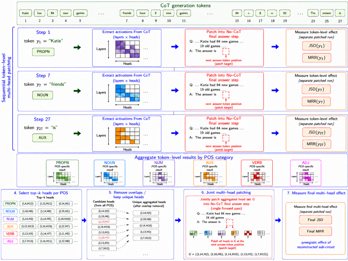
Standard activation patching methodologies are conventionally designed to intervene at a single, static token position. However, because CoT reasoning inherently unfolds over a sequence of multiple intermediate tokens, applying this standard setup directly is insufficient. Therefore, it is necessary to formulate a sequential patching approach (Appendix A, Algorithm 1). Building on this, we perform causal interventions using activation patching, where the outputs of attention heads from the clean run are injected into the corrupted run. Treating CoT as a multi-step process and operating under the hypothesis that CoT information is carried throughout the reasoning trajectory, we adopt a many-to-one patching strategy. For each source CoT token $t$ , layer $l$ , and head $h$ , we replace only that head’s output at the No-CoT next-token position immediately following the anchor “The answer is ”. Each $(t,l,h)$ intervention is evaluated in a separate forward pass, while all other head outputs remain unchanged (Appendix A, Algorithm 1, lines 9–22). This procedure produces a separate patched execution for each intervention.

However, analyzing these individual token-level results directly introduces significant noise, as the causal impact of a patched activation is often highly sensitive to the specific semantic and syntactic properties of tokens. To mitigate this noise and identify more robust computational patterns, we implement a Part-of-Speech (POS)-guided aggregation framework (Figure 1). We assign POS tags to each token in the reasoning trace and aggregate patching results across these linguistic categories (Appendix A, Algorithm 1, lines 23–33). Our goal in using POS-based aggregation is not to obscure individual POS-tag behavior, but to mitigate token-level noise and identify stable functional patterns across the CoT trajectory. By aggregating patching results across tokens sharing the same coarse POS category, we obtain more robust estimates of which heads consistently carry CoT-related signals. The selected POS categories and their corresponding head assignments are detailed in Appendix Tables 2 and 3.

This aggregation is crucial because CoT reasoning unfolds over multiple heterogeneous tokens, where a single token-level intervention may fail to capture the broader causal role of that segment in the reasoning trace. While semantic role labeling could offer an alternative categorical structure for this aggregation—a direction we identify for future research—POS tagging provides an initial framework for grouping tokens. This aggregation process transforms noisy, token-specific data into a single representative activation patching heatmap and a custom evaluation for each POS category. This, in turn, enables a fine-grained analysis of how causal signals are distributed across the reasoning process and helps identify specific heads that play a central role in processing different types of information within the CoT trajectory.

On a single NVIDIA RTX 6000 Ada GPU, the patching operation for one specific token position takes approximately 29.58 seconds using the TransformerLens library. Since our methodology involves scanning and patching all generated tokens within a CoT trace, the total analysis time per sample scales linearly with the length of the reasoning chain. Importantly, the overhead introduced by the POS-tagging step is exceptionally low: POS tagging for all 32 samples takes only 0.24 seconds in total, which is negligible compared to the computational cost of the repeated model forward passes required for these sequential evaluations.

Refer to caption — Figure 1: The figure illustrates our sequential activation patching setup (Appendix A, Algorithm 1). First, the model generates a Chain-of-Thought (CoT) token sequence, where each token $y_{t}$ corresponds to a generated reasoning token such as “Katie,” “friends,” or “is.” For each token, we extract the attention-head activations from the clean CoT run and patch them into the corrupted No-CoT run at the final answer generation position. The effect of each patched token is then measured using JSD and MRR. Since individual token-level effects can be noisy, the results are grouped by Part-of-Speech (POS) categories such as [VB], [NNP], [CD], [NNS], and [VBZ]. For each POS category, token-level patching results are aggregated into a layer-by-head heatmap, showing which attention heads consistently carry CoT-related information for that linguistic role.

3.6 Sequential Multi-Head Patching

Our sequential patching setup provides a comprehensive dataset containing evaluation metric results for all layer and attention-head combinations across each POS category (Appendix C.1, Figure 4). However, during our experiments, we observed that isolated interventions—patching only a single head at a time—failed to produce a meaningful shift in the model’s output toward CoT behavior. This indicates that CoT information is not carried by a single component in isolation; rather, it relies on a distributed representation formed by the coordinated interaction of multiple components across different functional roles.

Motivated by this observation, we implement a selection and merging strategy to reconstruct broader CoT-related sub-circuits (Appendix A, Algorithm 2). First, we identify the top- $k$ most influential attention heads for each individual POS category (e.g., those yielding the lowest JSD scores). Instead of evaluating these functional categories in isolation, we aggregate these category-specific top heads into a single global intervention set. During this aggregation, we implement a deduplication mechanism: if a specific attention head appears among the top candidates for multiple POS categories, we assign it exclusively to the category in which it achieves its best overall performance. This resolves intervention conflicts by ensuring that each shared head contributes only the activation state corresponding to its most effective functional role. Finally, we perform global multi-head joint patching using this aggregated set. We simultaneously extract the targeted activations for all uniquely assigned heads in the global set from the clean CoT run and jointly inject them into the corrupted No-CoT run during a single forward pass. By computing the final JSD and MRR on the resulting distribution, we measure the synergistic effect of the reconstructed sub-circuit.

This approach allows us to directly quantify how the collective integration of multiple POS-guided components drives the model’s internal representations toward the prompt-based CoT-induced reasoning trajectory.

To provide further evidence for our hypothesis that patched runs move toward a CoT reasoning trajectory, we introduce two control conditions: Sequential Multi-Head Cross Patching, which performs sequential multi-head patching across different problems, and Random-Activation Sequential Multi-Head Patching. Detailed explanations and corresponding pseudocode are provided in Appendix A, Algorithms 3 and 4.

3.7 Zero Ablation of Identified Attention-Head Sets

While activation patching highlights which attention heads carry sufficient information to shift the model’s behavior toward a CoT-like distribution, it does not strictly establish that these heads are necessary for the reasoning process. To examine whether the heads identified through our patching experiments constitute such critical overlapping sub-circuits, we design targeted zero-ablation experiments (Appendix A, Algorithm 5).

We systematically zero-ablate the attention heads identified from our previous Sequential Multi-Head Patching, Sequential Multi-Head Cross Patching, and Random-Activation Sequential Multi-Head Patching setups. To evaluate the functional role of these heads, we perform zero-ablation across three scenarios: Direct-Equation Prompting, where we ablate heads during raw arithmetic generation (e.g., 14 + 312 =) to test for overlap with fundamental calculation circuits; No-CoT Prompting, where we ablate heads during direct answer generation to test our hypothesis that these heads encompass core abstraction and calculation circuits; and CoT Prompting, where we continuously ablate the heads at every token-generation step to assess their necessity for maintaining reasoning states throughout the entire trajectory. We evaluate the overall functional degradation caused by the intervention across these three scenarios. If the ablation yields the anticipated performance drop, it provides evidence that the heads identified through our patching experiments contribute to the sub-circuits required to solve mathematical problems and that these sub-circuits are effectively recruited under CoT prompting. Conversely, we use the heads from the Random-Activation Sequential Multi-Head Patching setup and completely randomly selected head sets as control conditions to ensure that any observed degradation is specifically tied to the disruption of the targeted circuits rather than being a generalized artifact of network-wide perturbation.

4 Experimental Results

4.1 Patching Results

We evaluate our causal intervention framework on 32 SVAMP mathematical word problems using three activation patching setups: Sequential Multi-Head Patching, Sequential Multi-Head Cross Patching, and Random-Activation Sequential Multi-Head Patching. Intervention effects are evaluated using JSD and MRR. The aggregate JSD and MRR results are summarized in Figure 2 and Figure 3, respectively, while detailed instance-level results and explanations are provided in Appendix C.

Sequential Multi-Head Patching.

In Sequential Multi-Head Patching, POS-guided activations from the clean CoT run of a target question are injected into the No-CoT run of the same question. As shown in Figure 2 and Figure 3, this intervention produces the strongest improvement among the evaluated patching configurations. The patched executions move substantially closer to the clean CoT distribution and recover a meaningful portion of the CoT decision margin. These results indicate that jointly injecting structured, POS-guided multi-head activations can drive both the global output distribution and the local decision boundary toward CoT-like behavior.

Sequential Multi-Head Cross Patching.

In the cross-patching setup, source activations are taken from the CoT trace of a different randomly selected question and injected into the target question’s No-CoT execution. As summarized in the same figures, cross-patching also shifts the model toward the CoT reference, but the effect is weaker than in the same-question Sequential Multi-Head Patching setting. This reduction is expected because the source trace no longer contains the target question’s specific entities, numerical operands, or local semantic structure. Nevertheless, the fact that cross-patching still produces a non-trivial improvement suggests that the selected heads encode partially reusable reasoning-support patterns rather than only problem-specific content.

Random-Activation Sequential Multi-Head Patching.

Random-Activation Sequential Multi-Head Patching serves as a control condition in which randomly generated activation tensors are injected instead of actual CoT activations. As shown in Figure 2 and Figure 3, this intervention fails to reproduce the improvements obtained by the targeted patching methods. The random control therefore supports the interpretation that the observed effects are not caused solely by arbitrary perturbations or generic sensitivity of attention heads, but are associated with structured CoT-related signals carried by the selected components.

4.2 Zero Ablation Results

Experiment	Metric	Equation Prompt	No-CoT Prompt	CoT Prompt
		Accuracy	Accuracy	Accuracy
Normal Run	N/A	34.38%	31.25%	65.63%
Sequential Multi-Head Patching	JSD	9.38%	12.50%	0.00%
Sequential Multi-Head Patching	MRR	9.38%	9.38%	6.25%
Sequential Multi-Head Cross Patching	JSD	6.25%	6.25%	9.38%
Sequential Multi-Head Cross Patching	MRR	18.75%	12.50%	6.25%
Random-Activation Sequential Multi-Head Patching	JSD	18.75%	6.25%	12.50%
Random-Activation Sequential Multi-Head Patching	MRR	6.25%	12.50%	28.12%
Random $n$ -Head Selection	N/A	34.38%	15.63%	37.50%

Table 1: Zero-ablation accuracy results across prompting settings. The Normal Run row reports the original accuracy without ablation or patching. All other rows report accuracy after zero-ablating the corresponding selected head sets.

Table 1 reports the effect of zero-ablating the attention heads identified by our activation patching procedures. The analysis covers three distinct prompting settings: CoT Prompting, No-CoT Prompting, and Equation Prompting.

CoT Prompting.

The most pronounced degradation occurs in the CoT setting, highlighting the functional importance of the identified components. While the baseline CoT accuracy is $65.63\%$ , zero-ablating the heads selected via Sequential Multi-Head Patching using JSD reduces the model’s accuracy to $0.00\%$ . By comparison, ablating a randomly selected set of heads reduces accuracy to $37.50\%$ . It is important to distinguish this baseline from the Random-Activation Sequential Multi-Head Patching control, for which the corresponding ablations reduce accuracy to $12.50\%$ for JSD-based selection and $28.12\%$ for MRR-based selection. This condition is not a purely random baseline: because it ranks and selects heads according to their responses to injected random activations, it can preferentially identify perturbation-sensitive components. Nevertheless, the larger degradation observed for the targeted JSD-based Sequential Multi-Head Patching set provides causal evidence that these selected heads are functionally important for maintaining the CoT reasoning trajectory.

No-CoT and Equation Prompting.

In both the one-shot No-CoT and zero-shot Equation settings, targeted ablations generally produce larger accuracy drops than the Random $n$ -Head Selection baseline. In the No-CoT setting, accuracies decrease to $6.25\%$ – $12.50\%$ , compared with $15.60\%$ under random head selection. Similarly, in the Equation-only setting, accuracies fall to $6.25\%$ – $18.75\%$ , whereas the random baseline remains virtually unchanged at $34.40\%$ . These results indicate that the selected heads are not specific to the explicit CoT condition: even outside the CoT setting, they contribute to direct-answer reasoning and arithmetic computation. However, the results obtained from ablations based on Random-Activation Sequential Multi-Head Patching remain relatively close to those obtained from the other sequential patching variants. We attribute this proximity primarily to our current experimental constraints: the evaluation is conducted on only 32 instances, and the head-selection hyperparameter is restricted to $k=3$ per POS category. With such a narrow selection budget, the identified heads may capture only a partial subset of the relevant computational components. In the Equation-only setting, $k=3$ may be insufficient to capture the broader calculation circuit. In the No-CoT setting, this limitation may be even stronger, since direct-answer inference can depend on both abstraction and calculation mechanisms, as suggested by prior work on mathematical reasoning circuits (4). Consequently, the effects of the targeted ablations may overlap with those of the random-activation-derived head sets, limiting the separation between these conditions. Despite these constraints in the No-CoT and Equation settings, the particularly strong ablation effect observed in the CoT condition supports the hypothesis that our methodology identifies components that are important for sustaining step-by-step reasoning under CoT prompting. To better characterize this degradation beyond aggregate accuracy, we provide a qualitative breakdown of resulting failure modes—including final-anchor loss, exemplar contamination, and numerical corruption—in Appendix D.

5 Discussion and Conclusion

Our results support a mechanistic view of CoT prompting in which CoT does not merely add explanatory text, but helps steer the model’s internal computation toward a reasoning-compatible trajectory. Sequential activation patching moves No-CoT executions toward CoT behavior, suggesting that CoT-conditioned activations causally contribute to final-answer computation in our setting. However, this does not imply that every generated rationale token is a fully faithful explanation of the model’s internal reasoning. Rather, CoT appears to function as a useful internal control signal whose textual faithfulness may remain partial.

The same-question and cross-question patching results refine this interpretation. Stronger recovery under same-question patching indicates that part of the recovered computation is instance-sensitive, while the non-trivial gains under cross-question patching suggest that the discovered heads are not merely copying problem-specific operands or entities.

The need for joint multi-head interventions and the zero-ablation results further argue against a localized single-head account of CoT. Ablating the selected heads disrupts not only final-answer accuracy, but also final-answer anchoring, exemplar–target separation, answer-slot binding, and numerical generation. We therefore interpret the identified structure as a distributed reasoning-support sub-circuit rather than a pure reasoning-only circuit. Overall, our sequential activation patching framework provides evidence that CoT-related computation in the evaluated model on SVAMP relies on coordinated attention-head activity that supports both reasoning control and auxiliary mechanisms required for successful answer generation.

6 Limitations

One limitation of our work is that the analysis depends on how CoT-generated tokens are grouped before aggregation. We use POS tags as a practical labeling scheme, but alternative groupings, such as semantic-role labels or task-specific arithmetic labels, could cluster the reasoning tokens differently and lead to different head rankings. Second, our head-selection procedure relies on a fixed top- $k$ budget. Due to computational constraints, we do not perform a sensitivity analysis over different $k$ values, nor do we assign separate label-specific budgets. Therefore, the stability of the identified head sets under alternative selection policies remains an open question.

Another limitation is the scope of our empirical setting. Our experiments focus on mathematical word problems and one relatively small base model, so the extent to which the identified reasoning-support sub-circuits generalize to larger models, different architectures, specialized reasoning models, or non-mathematical reasoning tasks remains open. A further limitation is that our intervention metrics are computed at the first token of the final-answer span. This design provides a controlled and aligned decision point across CoT, No-CoT, and patched executions, but it does not fully evaluate the complete generated answer sequence.

Finally, the discovered heads should not be interpreted as a pure reasoning-only circuit. The ablation results suggest that these heads may also support related functions such as target-question grounding, exemplar separation, answer-slot binding, CoT formatting, and numerical generation. Thus, we interpret the identified structure as a distributed reasoning-support sub-circuit consisting of overlapping computational components that are dynamically recruited via CoT, rather than a complete or isolated reasoning circuit. Crucially, while our results suggest that these components are functionally important for CoT performance and less effectively recruited in No-CoT settings, we currently lack the granularity to isolate the distinct functional roles of individual heads within this overlapping ensemble. Determining which specific subsets of heads are responsible for abstraction, calculation, or other sub-tasks therefore remains an open challenge.

A promising direction for future work is to use the identified heads as a mechanistic prior for parameter-efficient fine-tuning. Since our interventions suggest that these heads participate in CoT-related reasoning-support computation, future studies could restrict PEFT modules, such as head-specific adapters or LoRA updates, to the corresponding attention-head subspaces instead of fine-tuning the entire model. Such a mechanistically informed PEFT strategy could reduce the number of trainable parameters while making the adaptation process more targeted and interpretable. However, because our ablation results indicate that the selected heads support overlapping functions such as answer anchoring, exemplar–target separation, answer-slot binding, and numerical generation, future work should first disentangle which subsets of heads are responsible for specific computational roles before treating them as isolated reasoning modules.

7 Ethics Statement

During the preparation of this manuscript, the authors utilized generative AI tools to assist in improving the linguistic quality, grammar, and overall readability of the text. AI tools were also employed to assist in the design and generation of figures and tables, facilitating the clear presentation of technical data. All AI-assisted outputs were subsequently reviewed, edited, and revised by the authors to ensure the technical accuracy of the arguments, the validity of the claims, and the precision of the visualized data. The authors certify that the final content, including all figures and tables, reflects their original research findings and intellectual contributions. The authors take full responsibility for the content of this manuscript and confirm that no original research data were generated or manipulated by AI tools.

References

Bentham et al. (2024) O. Bentham, N. Stringham, and A. Marasovic Chain-of-thought unfaithfulness as disguised accuracy. Trans. Mach. Learn. Res. 2024. External Links: Link Cited by: §2.1.
Cabannes et al. (2024) V. Cabannes, C. Arnal, W. Bouaziz, A. Yang, F. Charton, and J. Kempe Iteration head: a mechanistic study of chain-of-thought. External Links: 2406.02128, Link Cited by: §2.2.
Chen et al. (2026) X. Chen, A. Plaat, and N. van Stein How does chain of thought think? mechanistic interpretability of chain-of-thought reasoning with sparse autoencoding. In Fortieth AAAI Conference on Artificial Intelligence, Thirty-Eighth Conference on Innovative Applications of Artificial Intelligence, Sixteenth Symposium on Educational Advances in Artificial Intelligence, AAAI 2026, Singapore, January 20-27, 2026, S. Koenig, C. Jenkins, and M. E. Taylor (Eds.), pp. 30297–30305. External Links: Link, Document Cited by: §1, §3.3.1.
Cheng et al. (2025) Z. Cheng, M. Cao, L. Pishdad, Y. Cao, and J. C. K. Cheung Can llms reason abstractly over math word problems without cot? disentangling abstract formulation from arithmetic computation. External Links: 2505.23701, Link Cited by: §3.2, §4.2.
Dutta et al. (2024) S. Dutta, J. Singh, S. Chakrabarti, and T. Chakraborty How to think step-by-step: a mechanistic understanding of chain-of-thought reasoning. External Links: 2402.18312, Link Cited by: §1, §2.2.
Jacovi and Goldberg (2020) A. Jacovi and Y. Goldberg Towards faithfully interpretable nlp systems: how should we define and evaluate faithfulness?. External Links: 2004.03685, Link Cited by: §2.1.
Kojima et al. (2023) T. Kojima, S. S. Gu, M. Reid, Y. Matsuo, and Y. Iwasawa Large language models are zero-shot reasoners. External Links: 2205.11916, Link Cited by: §2.1.
Kudo et al. (2026) K. Kudo, Y. Aoki, T. Kuribayashi, S. Sone, M. Taniguchi, A. Brassard, K. Sakaguchi, and K. Inui LLMs faithfully and iteratively compute answers during cot: a systematic analysis with multi-step arithmetics. External Links: 2412.01113, Link Cited by: §2.1.
Lanham et al. (2023) T. Lanham, A. Chen, A. Radhakrishnan, B. Steiner, C. Denison, D. Hernandez, D. Li, E. Durmus, E. Hubinger, J. Kernion, K. Lukosiute, K. Nguyen, N. Cheng, N. Joseph, N. Schiefer, O. Rausch, R. Larson, S. McCandlish, S. Kundu, S. Kadavath, S. Yang, T. Henighan, T. Maxwell, T. Telleen-Lawton, T. Hume, Z. Hatfield-Dodds, J. Kaplan, J. Brauner, S. R. Bowman, and E. Perez Measuring faithfulness in chain-of-thought reasoning. CoRR abs/2307.13702. External Links: Link, Document, 2307.13702 Cited by: §1, §2.1.
Li et al. (2026) W. Li, F. Yang, A. Hazarika, S. A. Mehta, and K. Onoue When reasoning traces become performative: step-level evidence that chain-of-thought is an imperfect oversight channel. External Links: 2605.11746, Link Cited by: §2.1.
Mehrafarin et al. (2026) H. Mehrafarin, A. Parekh, and I. Konstas When chain-of-thought fails, the solution hides in the hidden states. External Links: 2604.23351, Link Cited by: §2.1.
Olsson et al. (2022) C. Olsson, N. Elhage, N. Nanda, N. Joseph, N. DasSarma, T. Henighan, B. Mann, A. Askell, Y. Bai, A. Chen, T. Conerly, D. Drain, D. Ganguli, Z. Hatfield-Dodds, D. Hernandez, S. Johnston, A. Jones, J. Kernion, L. Lovitt, K. Ndousse, D. Amodei, T. Brown, J. Clark, J. Kaplan, S. McCandlish, and C. Olah In-context learning and induction heads. External Links: 2209.11895, Link Cited by: §2.2.
Pan et al. (2026) L. Pan, J. Liang, J. Ye, M. Yang, X. Lu, and F. Zhu Opening the black box: a survey on the mechanisms of multi-step reasoning in large language models. External Links: 2601.14270, Link Cited by: §2.
Patel et al. (2021) A. Patel, S. Bhattamishra, and N. Goyal Are NLP models really able to solve simple math word problems?. CoRR abs/2103.07191. External Links: Link, 2103.07191 Cited by: §3.1.
Paul et al. (2024) D. Paul, R. West, A. Bosselut, and B. Faltings Making reasoning matter: measuring and improving faithfulness of chain-of-thought reasoning. In Findings of the Association for Computational Linguistics: EMNLP 2024, Miami, Florida, USA, November 12-16, 2024, Y. Al-Onaizan, M. Bansal, and Y. Chen (Eds.), Findings of ACL, pp. 15012–15032. External Links: Link, Document Cited by: §1, §2.1.
Pfau et al. (2024) J. Pfau, W. Merrill, and S. R. Bowman Let’s think dot by dot: hidden computation in transformer language models. External Links: 2404.15758, Link Cited by: §2.2.
Qwen et al. (2025) Qwen, A. Yang, B. Yang, B. Zhang, B. Hui, B. Zheng, B. Yu, C. Li, D. Liu, F. Huang, H. Wei, H. Lin, J. Yang, J. Tu, J. Zhang, J. Yang, J. Yang, J. Zhou, J. Lin, K. Dang, K. Lu, K. Bao, K. Yang, L. Yu, M. Li, M. Xue, P. Zhang, Q. Zhu, R. Men, R. Lin, T. Li, T. Tang, T. Xia, X. Ren, X. Ren, Y. Fan, Y. Su, Y. Zhang, Y. Wan, Y. Liu, Z. Cui, Z. Zhang, and Z. Qiu Qwen2.5 technical report. External Links: 2412.15115, Link Cited by: §1.
Stolfo et al. (2023) A. Stolfo, Y. Belinkov, and M. Sachan A mechanistic interpretation of arithmetic reasoning in language models using causal mediation analysis. External Links: 2305.15054, Link Cited by: §2.2.
Turpin et al. (2023) M. Turpin, J. Michael, E. Perez, and S. R. Bowman Language models don’t always say what they think: unfaithful explanations in chain-of-thought prompting. CoRR abs/2305.04388. External Links: Link, Document, 2305.04388 Cited by: §1.
Tutek et al. (2025) M. Tutek, F. Hashemi Chaleshtori, A. Marasovic, and Y. Belinkov Measuring chain of thought faithfulness by unlearning reasoning steps. In Proceedings of the 2025 Conference on Empirical Methods in Natural Language Processing, C. Christodoulopoulos, T. Chakraborty, C. Rose, and V. Peng (Eds.), Suzhou, China, pp. 9935–9960. External Links: Link, Document, ISBN 979-8-89176-332-6 Cited by: §2.1.
Wang et al. (2022) K. Wang, A. Variengien, A. Conmy, B. Shlegeris, and J. Steinhardt Interpretability in the wild: a circuit for indirect object identification in gpt-2 small. External Links: 2211.00593, Link Cited by: §2.2.
Wei et al. (2022) J. Wei, X. Wang, D. Schuurmans, M. Bosma, B. Ichter, F. Xia, E. H. Chi, Q. V. Le, and D. Zhou Chain-of-thought prompting elicits reasoning in large language models. In Proceedings of the 36th International Conference on Neural Information Processing Systems, NIPS ’22, Red Hook, NY, USA. External Links: ISBN 9781713871088 Cited by: §1, §2.1, §3.1.
Ye et al. (2026) D. Ye, M. Loffgren, O. Kotadia, and L. Wong Mechanistic evidence for faithfulness decay in chain-of-thought reasoning. External Links: 2602.11201, Link Cited by: §2.2.
Yeo et al. (2024) W. J. Yeo, R. Satapathy, and E. Cambria Towards faithful natural language explanations: a study using activation patching in large language models. External Links: 2410.14155, Link Cited by: §2.2.
Zaman and Srivastava (2026) K. Zaman and S. Srivastava Is chain-of-thought really not explainability? chain-of-thought can be faithful without hint verbalization. External Links: 2512.23032, Link Cited by: §1.
Zhang and Nanda (2024) F. Zhang and N. Nanda Towards best practices of activation patching in language models: metrics and methods. External Links: 2309.16042, Link Cited by: §1, §2.2, §3.
Zhao et al. (2026) Z. Zhao, Y. Koishekenov, X. Yang, N. Murray, and N. Cancedda Verifying chain-of-thought reasoning via its computational graph. External Links: 2510.09312, Link Cited by: §2.2.

Appendix A Algorithms

A.1 Sequential Multi-Head Cross Patching

In our preceding experiments, the source activations and the destination execution both originated from the same target question (i.e., patching CoT activations of Problem $A$ into the No-CoT execution of Problem $A$ ). While this same-question patching effectively identifies components associated with the reasoning trajectory, it introduces a potential confounding variable: it remains ambiguous whether the identified sub-circuits transfer a more general reasoning-support signal or simply carry problem-specific semantic information, such as particular numbers, entities, or operands unique to Problem $A$ .

To decouple problem-specific content from the more general Chain-of-Thought mechanism, we introduce Sequential Multi-Head Cross Patching (Appendix A, Algorithm 3). In this configuration, for a given target question ( $Q_{A}$ ), we randomly sample a distinct source question ( $Q_{B}$ ) from the dataset. We then extract the POS-guided, top-performing attention-head activations from the clean CoT execution of $Q_{B}$ and jointly inject them into the corrupted No-CoT execution of $Q_{A}$ . The resulting patched distribution is still evaluated against the clean reference distribution of the target question $Q_{A}$ .

This setup serves as a control for problem-specific information. If the patched attention heads predominantly encode local, problem-specific information, injecting activations from $Q_{B}$ into $Q_{A}$ should introduce semantic mismatch and reduce recovery toward the target CoT distribution. Conversely, if cross-question patching still yields recovery, this suggests that at least part of the selected activation structure transfers across instances rather than depending exclusively on problem-specific content. Cross-question recovery therefore provides evidence that the identified distributed components carry partially reusable reasoning-support signals beyond the source problem’s specific tokens.

Algorithm 1 Sequential Activation Patching and POS-Guided Aggregation

0: Target question

q

, source question

q^{\prime}

, CoT prompt

\mathcal{P}_{\mathrm{CoT}}

, No-CoT prompt

\mathcal{P}_{\mathrm{NoCoT}}

, model

M

, POS tagger

\mathcal{T}

, top-

k

parameter

1: Run

M(q,\mathcal{P}_{\mathrm{CoT}})

and store

D_{\mathrm{CoT}}

and

A_{\mathrm{CoT}}^{q}

2: Run

M(q,\mathcal{P}_{\mathrm{NoCoT}})

and store

D_{\mathrm{NoCoT}}

and

A_{\mathrm{NoCoT}}^{q}

3: Run

M(q^{\prime},\mathcal{P}_{\mathrm{CoT}})

and obtain CoT tokens

Y=(y_{1},\dots,y_{T})

4: Store source activations

A_{\mathrm{CoT}}^{q^{\prime}}

for all token positions, layers, and heads

5: Assign POS tags:

p_{t}\leftarrow\mathcal{T}(y_{t})

for

t=1,\dots,T

6: Compute baseline divergence once:

\mathrm{JSD}_{\mathrm{base}}\leftarrow\mathrm{JSD}(D_{\mathrm{CoT}},D_{\mathrm{NoCoT}})

8: Initialize

\mathcal{R}\leftarrow\emptyset

9: for each token position

t

10: for each layer

\ell

11: for each head

h

12: Patch:

13:

A_{\mathrm{NoCoT}}^{q}[\ell,h]\leftarrow A_{\mathrm{CoT}}^{q^{\prime}}[t,\ell,h]

14: Run forward pass

\rightarrow D_{\mathrm{patch}}^{(t,\ell,h)}

15: Compute:

16:

\mathrm{JSD}_{\mathrm{patch}}^{(t,\ell,h)}

17:

\mathrm{MRR}^{(t,\ell,h)}

18: Store:

19:

(p_{t},t,\ell,h,\mathrm{JSD}_{\mathrm{patch}}^{(t,\ell,h)},\mathrm{MRR}^{(t,\ell,h)})\rightarrow\mathcal{R}

20: end for

21: end for

22: end for

23: POS-Guided Aggregation:

24: Initialize

\mathcal{H}\leftarrow\emptyset

25: for each unique POS tag

p

Y

26:

\mathcal{R}_{p}\leftarrow

subset of records in

\mathcal{R}

with POS tag

p

27: for each head

(\ell,h)

28: Compute

\mu_{\mathrm{JSD}}\leftarrow

mean

\mathrm{JSD}_{\mathrm{patch}}

over

\mathcal{R}_{p}

29: Compute

\mu_{\mathrm{MRR}}\leftarrow

mean

\mathrm{MRR}

over

\mathcal{R}_{p}

30: end for

31:

\mathcal{H}_{p}\leftarrow

select top-

k

heads for

p

according to the chosen metric

32: Store

\mathcal{H}_{p}

\mathcal{H}

33: end for

34: return

\mathcal{R},\mathcal{H}

Algorithm 2 Sequential Multi-Head Patching

0: Record set

\mathcal{R}

, No-CoT run, CoT reference distribution

D_{\mathrm{CoT}}

, top-

k

parameter

1: for each POS tag

p

2: Collect all records in

\mathcal{R}

with POS tag

p

3: Rank candidate heads according to the chosen patching metric

4: (e.g., lower

\mathrm{JSD}_{\mathrm{patch}}

or higher

\mathrm{MRR}

)

5: Select the top-

k

heads for POS tag

p

\mathcal{H}_{p}\leftarrow\{(\ell_{1},h_{1}),(\ell_{2},h_{2}),\dots,(\ell_{k},h_{k})\}

7: end for

8: Initialize global selected-head set

\mathcal{G}\leftarrow\emptyset

9: for each POS tag

p

10: for each head

(\ell,h)\in\mathcal{H}_{p}

11: if

(\ell,h)\notin\mathcal{G}

then

12: Add

((\ell,h),p)

\mathcal{G}

13: else

14: Compare the existing POS assignment with the new POS assignment

15: Retain the assignment with the better metric value

16: end if

17: end for

18: end for

19: Extract the clean CoT activation associated with each

((\ell,h),p)\in\mathcal{G}

20: Jointly patch all uniquely assigned heads in

\mathcal{G}

into the No-CoT run

21: Run one patched forward pass and obtain

D_{\mathrm{patch}}^{\mathrm{multi}}

22: Compute:

23:

\mathrm{JSD}^{\mathrm{multi}}\leftarrow\mathrm{JSD}(D_{\mathrm{CoT}},D_{\mathrm{patch}}^{\mathrm{multi}})

24:

\mathrm{MRR}^{\mathrm{multi}}

25: return

\mathcal{G}

and the multi-head metric results

A.2 Random-Activation Sequential Multi-Head Patching

To assess whether the observed effects can be explained by arbitrary internal perturbations, we establish a Random-Activation Sequential Multi-Head Patching. In mechanistic interpretability, intervening on a model’s hidden states can sometimes inadvertently disrupt its default computational graph. This disruption might lead to unexpected distributional shifts that could be falsely interpreted as meaningful causal effects, raising the question of whether the model is actually utilizing CoT information or just reacting to random noise.

To rigorously rule out this null hypothesis, we replicate our multi-head patching procedure using randomly generated activation vectors in place of the actual CoT representations. As detailed in Algorithm 4, for each attention head, we generate a random activation tensor and inject it into the corrupted No-CoT run. We then evaluate these random interventions, rank the heads based on their accidental patching quality, and perform a joint multi-head patch using the top- $n$ random activations.

Algorithm 3 Sequential Multi-Head Cross Patching

0: Target question

Q_{A}

, source question

Q_{B}

, CoT prompt

\mathcal{P}_{\mathrm{CoT}}

, No-CoT prompt

\mathcal{P}_{\mathrm{NoCoT}}

, model

M

, POS tagger

\mathcal{T}

, top-

k

parameter

1: Run the clean target execution

M(Q_{A},\mathcal{P}_{\mathrm{CoT}})

and store

D_{\mathrm{CoT}}^{A}

2: Run the corrupted target execution

M(Q_{A},\mathcal{P}_{\mathrm{NoCoT}})

and store

D_{\mathrm{NoCoT}}^{A}

and

A_{\mathrm{NoCoT}}^{A}

3: Run

M(Q_{B},\mathcal{P}_{\mathrm{CoT}})

and obtain source CoT tokens

Y^{B}=(y_{1},\dots,y_{T})

4: Store source activations

A_{\mathrm{CoT}}^{B}

for all token positions, layers, and heads

5: Assign POS tags:

p_{t}\leftarrow\mathcal{T}(y_{t})

for each

y_{t}\in Y^{B}

6: Initialize record set

\mathcal{R}\leftarrow\emptyset

7: Initialize global assignment map

\mathcal{G}\leftarrow\emptyset

8: for each token position

t

9: for each layer

\ell

10: for each head

h

11: Patch:

12:

A_{\mathrm{NoCoT}}^{A}[\ell,h]\leftarrow A_{\mathrm{CoT}}^{B}[t,\ell,h]

13: Run the patched forward pass and obtain

D_{\mathrm{patch}}^{(t,\ell,h)}

14: Compute:

15:

\mathrm{JSD}_{\mathrm{patch}}^{(t,\ell,h)}\leftarrow\mathrm{JSD}\left(D_{\mathrm{CoT}}^{A},D_{\mathrm{patch}}^{(t,\ell,h)}\right)

16:

\mathrm{MRR}^{(t,\ell,h)}

17: Store:

18:

(p_{t},t,\ell,h,\mathrm{JSD}_{\mathrm{patch}}^{(t,\ell,h)},\mathrm{MRR}^{(t,\ell,h)})\rightarrow\mathcal{R}

19: end for

20: end for

21: end for

22: for each unique POS tag

p

Y^{B}

23:

\mathcal{R}_{p}\leftarrow

subset of records in

\mathcal{R}

with POS tag

p

24: Compute the mean patching metric for each candidate head

(\ell,h)

within

\mathcal{R}_{p}

25: Select the top-

k

heads

\mathcal{H}_{p}

according to the chosen metric

26: for each head

(\ell,h)\in\mathcal{H}_{p}

27: if

(\ell,h)

is not assigned in

\mathcal{G}

then

28: Assign

((\ell,h),p)

\mathcal{G}

29: else

30: Compare the existing POS assignment with the new POS assignment

31: Retain the assignment with the better metric value

32: end if

33: end for

34: end for

35: Let

\widehat{\mathcal{H}}\leftarrow\mathrm{keys}(\mathcal{G})

denote the final deduplicated head set

36: Extract the source CoT activation associated with each

((\ell,h),p)\in\mathcal{G}

37: Jointly patch all heads in

\widehat{\mathcal{H}}

into the target No-CoT run

38: Run one joint patched forward pass and obtain

D_{\mathrm{patch}}^{\mathrm{cross}}

39: Compute:

40:

\mathrm{JSD}^{\mathrm{cross}}\leftarrow\mathrm{JSD}\left(D_{\mathrm{CoT}}^{A},D_{\mathrm{patch}}^{\mathrm{cross}}\right)

41:

\mathrm{MRR}^{\mathrm{cross}}

42: return

\mathcal{G}

\widehat{\mathcal{H}}

\mathrm{JSD}^{\mathrm{cross}}

, and

\mathrm{MRR}^{\mathrm{cross}}

Algorithm 4 Random-Activation Sequential Multi-Head Patching

0: Target question

q

, CoT prompt

\mathcal{P}_{\mathrm{CoT}}

, No-CoT prompt

\mathcal{P}_{\mathrm{NoCoT}}

, model

M

, integer

n

1: Run

M(q,\mathcal{P}_{\mathrm{CoT}})

and store output distribution

D_{\mathrm{CoT}}

2: Run

M(q,\mathcal{P}_{\mathrm{NoCoT}})

and store output distribution

D_{\mathrm{NoCoT}}

and activations

A_{\mathrm{NoCoT}}^{q}

3: Compute baseline divergence once:

\mathrm{JSD}_{\mathrm{base}}\leftarrow\mathrm{JSD}\left(D_{\mathrm{CoT}},D_{\mathrm{NoCoT}}\right)

5: Initialize result set

\mathcal{R}_{\mathrm{rand}}\leftarrow\emptyset

6: Initialize random activation table

\mathcal{Z}\leftarrow\emptyset

7: for each layer

\ell

8: for each head

h

9: Generate a random activation

z_{\ell,h}

for head

(\ell,h)

10: Store

z_{\ell,h}

\mathcal{Z}

11: Patch the No-CoT run with

z_{\ell,h}

at head

(\ell,h)

12: Run the patched forward pass and obtain

D_{\mathrm{patch}}^{(\ell,h)}

13: Compute:

14:

\mathrm{JSD}_{\mathrm{patch}}^{(\ell,h)}\leftarrow\mathrm{JSD}\left(D_{\mathrm{CoT}},D_{\mathrm{patch}}^{(\ell,h)}\right)

15:

\mathrm{MRR}^{(\ell,h)}

16: Store:

17:

(\ell,h,\mathrm{JSD}_{\mathrm{patch}}^{(\ell,h)},\mathrm{MRR}^{(\ell,h)})\rightarrow\mathcal{R}_{\mathrm{rand}}

18: end for

19: end for

20: Rank all heads in

\mathcal{R}_{\mathrm{rand}}

according to the chosen patching metric

21: (e.g., lower

\mathrm{JSD}_{\mathrm{patch}}

or higher

\mathrm{MRR}

)

22: Select the top-

n

heads:

23:

\mathcal{H}_{\mathrm{top}\text{-}n}\leftarrow\{(\ell_{1},h_{1}),\dots,(\ell_{n},h_{n})\}

24: Jointly patch the No-CoT run using the stored random activations:

25:

\{z_{\ell,h}:(\ell,h)\in\mathcal{H}_{\mathrm{top}\text{-}n}\}

26: Run one joint patched forward pass and obtain

D_{\mathrm{patch}}^{\mathrm{top}\text{-}n}

27: Compute:

28:

\mathrm{JSD}^{\mathrm{top}\text{-}n}\leftarrow\mathrm{JSD}\left(D_{\mathrm{CoT}},D_{\mathrm{patch}}^{\mathrm{top}\text{-}n}\right)

29:

\mathrm{MRR}^{\mathrm{top}\text{-}n}

30: return

\mathcal{H}_{\mathrm{top}\text{-}n}

\mathcal{R}_{\mathrm{rand}}

D_{\mathrm{patch}}^{\mathrm{top}\text{-}n}

\mathrm{JSD}^{\mathrm{top}\text{-}n}

, and

\mathrm{MRR}^{\mathrm{top}\text{-}n}

Algorithm 5 Zero Ablation of Patching-Selected Heads

0: Dataset

\mathcal{D}

, CoT prompt

\mathcal{P}_{\mathrm{CoT}}

, No-CoT prompt

\mathcal{P}_{\mathrm{NoCoT}}

, direct-equation prompt

\mathcal{P}_{\mathrm{Eq}}

, model

M

, selected-head set

\mathcal{H}_{\mathrm{sel}}

1: Initialize No-CoT results

\mathcal{R}_{\mathrm{NoCoT}}\leftarrow\emptyset

2: Initialize CoT results

\mathcal{R}_{\mathrm{CoT}}\leftarrow\emptyset

3: Initialize direct-equation results

\mathcal{R}_{\mathrm{Eq}}\leftarrow\emptyset

4: for each question

q\in\mathcal{D}

5: Obtain patching-selected heads

\mathcal{H}_{\mathrm{sel}}^{q}

for question

q

6: Sample matched random heads

\mathcal{H}_{\mathrm{rand}}^{q}

such that

|\mathcal{H}_{\mathrm{rand}}^{q}|=|\mathcal{H}_{\mathrm{sel}}^{q}|

8: Direct-Equation Ablation:

9: Construct the equation-only input

e_{q}

corresponding to question

q

10: Run

M(e_{q},\mathcal{P}_{\mathrm{Eq}})

and store the original equation prediction

\hat{y}_{\mathrm{Eq}}

11: Zero-ablate all heads in

\mathcal{H}_{\mathrm{sel}}^{q}

during direct-equation inference

12: Run the selected-head-ablated equation forward pass and obtain

\hat{y}_{\mathrm{Eq}}^{\mathrm{sel}}

13: Zero-ablate all heads in

\mathcal{H}_{\mathrm{rand}}^{q}

during direct-equation inference

14: Run the random-head-ablated equation forward pass and obtain

\hat{y}_{\mathrm{Eq}}^{\mathrm{rand}}

15: Store:

(q,\hat{y}_{\mathrm{Eq}},\hat{y}_{\mathrm{Eq}}^{\mathrm{sel}},\hat{y}_{\mathrm{Eq}}^{\mathrm{rand}})\rightarrow\mathcal{R}_{\mathrm{Eq}}

16: No-CoT Ablation:

17: Run

M(q,\mathcal{P}_{\mathrm{NoCoT}})

and store the original No-CoT prediction

\hat{y}_{\mathrm{NoCoT}}

18: Zero-ablate all heads in

\mathcal{H}_{\mathrm{sel}}^{q}

during No-CoT inference

19: Run the selected-head-ablated No-CoT forward pass and obtain

\hat{y}_{\mathrm{NoCoT}}^{\mathrm{sel}}

20: Zero-ablate all heads in

\mathcal{H}_{\mathrm{rand}}^{q}

during No-CoT inference

21: Run the random-head-ablated No-CoT forward pass and obtain

\hat{y}_{\mathrm{NoCoT}}^{\mathrm{rand}}

22: Store:

(q,\hat{y}_{\mathrm{NoCoT}},\hat{y}_{\mathrm{NoCoT}}^{\mathrm{sel}},\hat{y}_{\mathrm{NoCoT}}^{\mathrm{rand}})\rightarrow\mathcal{R}_{\mathrm{NoCoT}}

23: CoT Ablation:

24: Run

M(q,\mathcal{P}_{\mathrm{CoT}})

and store the original CoT prediction

\hat{y}_{\mathrm{CoT}}

25: Generate the CoT token sequence:

Y=(y_{1},y_{2},\dots,y_{T})

26: for each generated CoT token

y_{t}\in Y

27: Obtain token-specific selected heads

\mathcal{H}_{\mathrm{sel}}^{q,t}

28: Zero-ablate all heads in

\mathcal{H}_{\mathrm{sel}}^{q,t}

during generation of token

y_{t}

29: end for

30: Store the selected-head-ablated CoT prediction

\hat{y}_{\mathrm{CoT}}^{\mathrm{sel}}

31: for each generated CoT token

y_{t}\in Y

32: Sample matched random heads

\mathcal{H}_{\mathrm{rand}}^{q,t}

such that

33:

|\mathcal{H}_{\mathrm{rand}}^{q,t}|=|\mathcal{H}_{\mathrm{sel}}^{q,t}|

34: Zero-ablate all heads in

\mathcal{H}_{\mathrm{rand}}^{q,t}

during generation of token

y_{t}

35: end for

36: Store the random-head-ablated CoT prediction

\hat{y}_{\mathrm{CoT}}^{\mathrm{rand}}

37: Store:

(q,\hat{y}_{\mathrm{CoT}},\hat{y}_{\mathrm{CoT}}^{\mathrm{sel}},\hat{y}_{\mathrm{CoT}}^{\mathrm{rand}})\rightarrow\mathcal{R}_{\mathrm{CoT}}

38: end for

39: Compute original accuracies for Direct-Equation, No-CoT, and CoT prompting

40: Compute selected-head ablation accuracies for all three prompting conditions

41: Compute random-head ablation accuracies for all three prompting conditions

42: return

\mathcal{R}_{\mathrm{Eq}}

\mathcal{R}_{\mathrm{NoCoT}}

\mathcal{R}_{\mathrm{CoT}}

, original accuracies, selected-head ablation accuracies, and random-head ablation accuracies

Appendix B Evaluation Metrics Details

In our activation patching experiments, we use two primary metrics to quantify the causal effect of interventions on attention-head activations: Jensen–Shannon Divergence (JSD) and Margin Recovery Ratio (MRR). This section provides the formal definitions and interpretation guidelines for both metrics.

B.1 Jensen–Shannon Divergence (JSD)

We use Jensen–Shannon Divergence (JSD) to measure the divergence between the next-token probability distribution of the patched model, $P_{\text{patch}}$ , and that of the clean Chain-of-Thought (CoT) execution, $P_{\text{CoT}}$ . JSD is a symmetric and smoothed variant of the Kullback–Leibler (KL) divergence, defined as:

\mathrm{JSD}\left(P_{\text{patch}},P_{\text{CoT}}\right)=\frac{1}{2}\mathrm{KL}\left(P_{\text{patch}}\parallel M\right)+\frac{1}{2}\mathrm{KL}\left(P_{\text{CoT}}\parallel M\right),

where

M=\frac{1}{2}\left(P_{\text{patch}}+P_{\text{CoT}}\right)

is the pointwise mixture distribution, and $\mathrm{KL}$ denotes the standard Kullback–Leibler divergence. Interpretation of the JSD Scale: Unlike KL divergence, JSD is bounded. Because we compute the KL divergence using the natural logarithm (base $e$ ), the JSD values in our experiments lie within the range $[0,\ln 2]$ , where $\ln 2\approx 0.693$ .

•

$\mathrm{JSD}=0$ indicates that the patched and clean CoT next-token distributions are identical at the evaluated decoding position.
•

Higher JSD values, approaching the theoretical maximum of $\ln 2\approx 0.693$ , indicate greater divergence between the patched and clean CoT distributions. Accordingly, lower JSD values indicate that the intervention moves the model’s next-token distribution closer to the clean CoT reference.

B.2 Margin Recovery Ratio (MRR)

To capture decision-level effects, we define a logit-based margin metric. Let $t^{*}$ denote the target answer token at the evaluated decoding position, and let $z(t)$ denote the logit assigned to token $t$ . The margin $M$ is defined as:

M=z(t^{*})-\max_{t\neq t^{*}}z(t).

We compute this margin for the clean CoT reference, $M_{\text{CoT}}$ , the corrupted No-CoT baseline, $M_{\text{NoCoT}}$ , and the patched execution, $M_{\text{patch}}$ . The Margin Recovery Ratio (MRR) is then defined as:

\mathrm{MRR}=\frac{M_{\text{patch}}-M_{\text{NoCoT}}}{M_{\text{CoT}}-M_{\text{NoCoT}}}.

The Margin Recovery Ratio is defined when $M_{\text{CoT}}\neq M_{\text{NoCoT}}$ . This ensures that the denominator represents a non-zero difference between the clean CoT and No-CoT decision margins. When $M_{\text{CoT}}=M_{\text{NoCoT}}$ , the ratio is undefined because there is no margin difference between the two reference conditions to recover. Interpretation of the MRR Scale: MRR measures how much of the CoT–No-CoT margin difference is recovered by the patching intervention. Its values are interpreted as follows:

•

$\mathrm{MRR}<0$ : The patched execution moves the target-token margin in the opposite direction from the clean CoT reference relative to the No-CoT baseline.
•

$\mathrm{MRR}=0$ : The patched execution recovers none of the CoT–No-CoT margin difference.
•

$0<\mathrm{MRR}<1$ : The intervention partially recovers the CoT–No-CoT margin difference.
•

$\mathrm{MRR}=1$ : The patched execution matches the clean CoT decision margin.
•

$\mathrm{MRR}>1$ : The patched execution exceeds the clean CoT decision margin in the direction of the target answer token.

Appendix C Sequential Multi-Head Patching Results

ID	Type	Eq	Stat	Logit (No $\rightarrow$ Pat.)		Prob (No $\rightarrow$ Pat.)		JSD
chal-961	Addition	1	$\times\times$	23.61 $\rightarrow$	28.68	36.2% $\rightarrow$	97.8%	0.0072
Heads: L16H13[NNP], L16H10[CD], L13H12[:], L13H0[NNP], L14H5[VBZ], L14H10[JJ], L12H13[VBZ], L14H13[.], L16H8[.], L14H1[NN], L13H4[NN], L12H0[JJ], L15H1[NNS], L13H7[PRP$]
chal-569	Addition	1	$\checkmark\times$	21.87 $\rightarrow$	22.13	27.7% $\rightarrow$	21.9%	0.4047
Heads: L10H7[:], L13H12[.], L8H7[:], L14H5[IN], L10H6[NN], L14H8[NN], L8H3[VBD], L10H12[JJ], L16H10[TO], L14H4[JJ], L9H2[.], L14H2[CD], L10H3[CD], L13H10[NNS], L9H1[IN], L10H9[IN], L13H13[CC], L13H4[DT], L13H1[DT], L12H4[VBZ], L14H10[VBZ], L11H5[VBZ]
chal-290	Addition	1	$\times\times$	22.23 $\rightarrow$	22.82	28.2% $\rightarrow$	40.6%	0.2662
Heads: L13H12[VBD], L20H10[IN], L15H13[:], L14H10[RB], L14H7[CD], L20H12[.], L14H13[.], L14H5[NNS], L13H13[DT], L12H12[TO], L12H6[,], L17H8[VBZ]
chal-821	Addition	1	$\checkmark\times$	22.63 $\rightarrow$	25.13	45.4% $\rightarrow$	85.5%	0.0525
Heads: L13H12[IN], L4H12[NNP], L17H7[:], L14H12[NNP], L14H2[CD], L14H5[CD], L14H11[CD], L12H10[.], L14H10[VBZ]
chal-451	Common-Divis	1	$\checkmark\times$	22.14 $\rightarrow$	24.91	30.7% $\rightarrow$	91.5%	0.0285
Heads: L11H3[VBZ], L4H12[:], L11H0[:], L10H6[CD], L12H13[NNS], L14H5[PRP], L13H3[IN], L11H5[NN], L14H7[CD], L15H13[CD], L10H12[.], L13H6[NNS], L10H7[CC], L13H10[CC], L12H0[NN], L14H8[DT], L12H8[DT]
chal-970	Common-Divis	1	$\checkmark\times$	21.38 $\rightarrow$	23.09	16.4% $\rightarrow$	49.1%	0.2163
Heads: L13H3[NN], L13H12[PRP$], L16H7[CD], L12H13[CC], L14H10[CC], L15H1[NN], L22H7[VBZ], L14H5[VBZ], L16H11[.], L16H13[.], L14H13[.], L14H12[PRP$]
chal-215	Common-Divis	1	$\checkmark\times$	22.61 $\rightarrow$	19.05	80.6% $\rightarrow$	98.8%	0.0038
Heads: L13H6[:], L13H12[DT], L23H1[NN], L15H6[IN], L14H8[VBZ], L16H13[.], L13H1[CD], L22H0[CD], L13H10[CD], L7H13[JJ], L18H9[VB]
chal-160	Common-Divis	1	$\times\times$	21.85 $\rightarrow$	24.60	14.7% $\rightarrow$	79.0%	0.0664
Heads: L10H6[:], L16H8[CC], L16H13[CD], L8H7[EX], L15H12[VBP], L14H10[CD], L22H7[.], L13H3[NN], L15H10[CC], L14H7[DT], L14H12[NN], L12H0[,], L13H10[,], L14H8[JJ], L8H3[VBN]
chal-76	Multiplicati	1	$\times\times$	23.77 $\rightarrow$	20.01	88.3% $\rightarrow$	99.3%	0.0021
Heads: L14H10[:], L17H7[PRP], L18H9[NNS], L23H1[NN], L18H3[DT], L14H7[.], L22H7[VBZ], L14H13[.], L14H9[.], L22H0[CD]
chal-854	Multiplicati	1	$\checkmark\times$	18.52 $\rightarrow$	20.82	1.3% $\rightarrow$	4.5%	0.5954
Heads: L12H0[CD], L13H8[:], L16H7[:], L14H10[NN], L15H13[NN], L14H13[VBZ], L13H3[VBZ], L10H6[CD], L16H12[DT]
chal-196	Multiplicati	1	$\times\times$	20.80 $\rightarrow$	23.81	39.9% $\rightarrow$	59.1%	0.1636
Heads: L14H10[:], L13H12[NN], L8H7[PRP$], L9H2[NN], L12H0[NN], L13H1[NNS], L13H4[NNS], L16H7[.], L14H7[RB], L12H2[PRP$], L9H4[,], L11H8[VB], L13H6[VBZ], L6H9[VBZ]
chal-12	Multiplicati	1	$\checkmark\checkmark$	23.75 $\rightarrow$	23.88	75.2% $\rightarrow$	83.1%	0.0618
Heads: L16H8[CD], L16H10[.], L13H12[VBZ], L13H1[NN], L20H8[CD], L16H7[CD], L14H1[NNS], L16H13[IN], L6H9[IN], L10H6[NN]
chal-163	Subtraction	1	$\times\times$	20.37 $\rightarrow$	20.07	8.0% $\rightarrow$	2.6%	0.6303
Heads: L16H10[IN], L16H6[DT], L15H5[NNS], L10H6[PRP], L14H13[NN], L14H2[CD], L16H8[.], L14H10[CD], L14H9[DT], L14H5[JJ], L14H3[RBR]
chal-514	Subtraction	1	$\times\times$	22.31 $\rightarrow$	23.18	17.7% $\rightarrow$	80.1%	0.0697
Heads: L12H0[VBZ], L14H1[RBR], L14H13[CD], L9H10[NN], L10H6[CD], L16H0[.], L16H11[.], L14H5[RBR]
chal-954	Subtraction	1	$\checkmark\times$	22.90 $\rightarrow$	25.60	44.6% $\rightarrow$	96.2%	0.0124
Heads: L14H10[.], L21H9[VBZ], L14H1[CD], L14H7[CD], L18H9[.], L11H12[CD], L9H1[NN], L13H9[NN], L2H0[NN], L22H7[VBZ], L16H6[DT], L11H0[VBZ]
chal-83	Subtraction	1	$\times\times$	20.75 $\rightarrow$	21.81	6.6% $\rightarrow$	25.2%	0.3642
Heads: L16H8[.], L22H7[.], L16H7[.], L10H6[PRP], L8H3[PRP], L12H0[CD], L16H11[NN], L20H9[NNS], L12H4[DT]
chal-21	Addition	2	$\checkmark\times$	21.14 $\rightarrow$	22.81	25.9% $\rightarrow$	78.1%	0.0819
Heads: L14H13[NNP], L14H1[.], L13H3[NNS], L15H3[CD], L14H10[VBZ], L22H7[.], L13H12[DT]
chal-129	Addition	2	$\checkmark\times$	21.62 $\rightarrow$	22.65	17.5% $\rightarrow$	55.1%	0.1875
Heads: L13H8[:], L12H0[NNS], L16H8[IN], L15H13[NN], L16H7[NNS], L14H7[.], L14H5[.], L14H13[.], L14H9[DT]
chal-587	Addition	2	$\times\times$	21.15 $\rightarrow$	25.78	21.9% $\rightarrow$	91.3%	0.0294
Heads: L12H2[.], L13H3[CD], L12H8[:], L10H7[VBD], L4H12[EX], L8H5[DT], L16H8[.], L14H13[.], L12H6[CD], L7H13[NN], L12H13[NN], L14H7[NNS], L10H3[IN], L10H11[VBZ], L22H7[VBZ]
chal-254	Addition	2	$\checkmark\times$	23.73 $\rightarrow$	23.41	47.7% $\rightarrow$	48.3%	0.2230
Heads: L13H3[:], L10H6[:], L14H13[:], L13H4[DT], L14H1[CD], L4H12[VBD], L13H7[VBD], L12H13[CD], L8H7[NNS], L9H1[IN], L17H7[PRP], L5H6[DT], L22H7[VBZ], L15H1[VBZ]
chal-28	Common-Divis	2	$\times\times$	18.66 $\rightarrow$	20.06	1.3% $\rightarrow$	9.8%	0.4992
Heads: L16H13[CD], L14H9[VBZ], L16H11[CD], L14H10[CD], L14H13[NN], L13H6[VBD], L14H7[CC], L15H9[.], L15H7[.], L13H1[NNS], L15H10[CC], L22H7[VBZ]
chal-906	Common-Divis	2	$\checkmark\times$	20.69 $\rightarrow$	22.96	7.3% $\rightarrow$	57.5%	0.1740
Heads: L8H7[POS], L15H6[IN], L3H8[:], L10H6[NN], L13H7[IN], L14H7[.], L13H3[CD], L15H13[VBZ], L16H10[.], L14H5[RB], L12H13[RB]
chal-829	Common-Divis	2	$\checkmark\times$	22.49 $\rightarrow$	24.45	28.1% $\rightarrow$	91.6%	0.0275
Heads: L14H1[:], L14H10[NN], L13H8[:], L15H1[NNP], L11H12[NNS], L16H8[.], L10H6[CD], L14H7[NN], L12H6[IN], L14H8[DT], L22H7[VBZ], L14H5[VBZ]
chal-33	Common-Divis	2	$\checkmark\times$	22.35 $\rightarrow$	22.70	31.7% $\rightarrow$	29.0%	0.3436
Heads: L21H9[.], L10H6[:], L4H12[:], L16H11[IN], L5H9[EX], L13H3[CD], L14H7[.], L14H5[.], L14H10[DT], L14H1[NNS], L0H1[NNS], L8H3[DT], L22H7[VBZ], L15H9[VBZ]
chal-596	Multiplicati	2	$\checkmark\times$	20.96 $\rightarrow$	21.44	6.4% $\rightarrow$	16.3%	0.4535
Heads: L15H8[:], L15H12[:], L13H3[NN], L15H7[NNS], L12H0[VBZ], L23H1[NN], L16H11[CD], L22H7[.], L16H6[.], L16H7[CD], L22H6[CD], L14H12[IN]
chal-674	Multiplicati	2	$\checkmark\times$	21.92 $\rightarrow$	19.69	42.9% $\rightarrow$	5.1%	0.5896
Heads: L16H10[VBZ], L16H7[:], L16H6[:], L14H10[NN], L16H11[.], L16H8[.], L14H0[CD], L10H6[RB], L17H7[,], L20H8[,], L12H4[MD], L14H8[DT], L15H7[DT]
chal-859	Multiplicati	2	$\times\times$	20.36 $\rightarrow$	27.43	19.3% $\rightarrow$	49.0%	0.2201
Heads: L10H6[:], L14H10[CD], L16H6[NNS], L13H3[NN], L14H3[NN], L15H5[RB], L12H6[VBZ], L15H12[VBZ], L19H11[CD], L14H1[DT], L13H8[.], L18H3[CD], L14H2[IN], L9H1[IN], L15H0[PRP$]
chal-847	Multiplicati	2	$\checkmark\times$	20.58 $\rightarrow$	21.94	16.4% $\rightarrow$	19.6%	0.4247
Heads: L13H8[:], L16H10[NN], L22H7[IN], L14H10[PRP], L12H0[IN], L5H6[NN], L16H11[.], L14H1[VBZ]
chal-193	Subtraction	2	$\checkmark\times$	21.19 $\rightarrow$	19.81	23.9% $\rightarrow$	2.5%	0.6303
Heads: L13H12[.], L14H9[:], L10H3[VBG], L13H13[IN], L13H1[CD], L13H4[VBZ], L14H13[.], L14H7[CD], L12H10[VBZ], L4H12[DT], L14H2[VBG], L14H11[PRP], L12H0[VB], L5H9[VB], L15H1[TO], L23H12[RBR]
chal-889	Subtraction	2	$\checkmark\times$	20.51 $\rightarrow$	22.94	8.1% $\rightarrow$	74.5%	0.0926
Heads: L14H1[IN], L16H7[IN], L15H8[NNS], L14H13[.], L22H7[.], L16H11[.], L14H10[IN], L14H5[NNS], L14H7[NN], L4H12[PRP], L16H0[VB], L14H8[RBR], L16H2[DT]
chal-622	Subtraction	2	$\checkmark\times$	21.09 $\rightarrow$	22.12	20.6% $\rightarrow$	36.7%	0.2928
Heads: L12H6[:], L14H10[:], L14H9[DT], L15H3[VB], L14H7[VBZ], L16H11[.], L16H7[CD], L16H8[CD], L12H12[NNS], L21H9[VBN], L16H13[TO], L13H8[DT], L15H2[RB], L22H7[VBZ]
chal-462	Subtraction	2	$\checkmark\times$	20.45 $\rightarrow$	22.31	6.5% $\rightarrow$	10.1%	0.5123
Heads: L16H8[TO], L14H10[.], L10H6[:], L16H11[PRP], L12H0[CD], L15H13[NNS], L14H8[CD], L14H9[NN], L22H7[VBZ]

Table 2: Detailed results of Sequential Multi-Head Patching using JSD across 32 SVAMP instances. The Stat column indicates correct (✓) or incorrect (

\times

) answers for CoT (left) and No-CoT (right) prompting. The Eq column indicates how many operations the question includes. Logit and probability shifts represent values before and after patching attention head outputs into the No-CoT execution. Lower JSD values denote a closer distributional alignment with the clean CoT run. The Heads sub-row lists the aggregated sets of the most influential attention heads, selected based on their specific POS tags for each respective problem. The notation format for these elements indicates the layer number, head number, and the corresponding POS category (e.g., L15H3[VB] refers to Layer 15, Head 3, and POS category VB). The average final JSD across all multi-head patching instances is 0.2415.

T-ID	S-ID	T-Stat	S-Stat	Logit (No $\rightarrow$ Pat.)		Prob (No $\rightarrow$ Pat.)		JSD
chal-961	chal-674	$\times\times$	$\checkmark$	23.61 $\rightarrow$	22.07	36.2% $\rightarrow$	27.1%	0.3626
Cross-Heads: L12H0[CD], L14H5[.], L15H1[:], L14H10[MD], L14H8[DT], L12H12[VBP], L14H13[.], L14H1[NNS], L13H1[,], L8H3[VBZ]
chal-569	chal-514	$\checkmark\times$	$\times$	21.87 $\rightarrow$	23.26	27.7% $\rightarrow$	55.2%	0.1864
Cross-Heads: L14H5[.], L10H7[:], L13H12[CD], L11H3[NN], L14H8[NN], L14H10[VBZ], L13H4[DT], L13H6[CD], L15H1[NNS], L8H3[IN], L13H1[DT]
chal-290	chal-33	$\times\times$	$\checkmark$	22.23 $\rightarrow$	22.73	28.2% $\rightarrow$	52.3%	0.1993
Cross-Heads: L13H12[.], L15H8[:], L20H10[NNS], L14H10[.], L14H13[.], L14H1[CD], L12H0[CD], L15H10[NNS], L20H12[IN], L13H1[IN], L14H7[DT], L22H7[VBZ]
chal-821	chal-674	$\checkmark\times$	$\checkmark$	22.63 $\rightarrow$	25.89	45.4% $\rightarrow$	88.5%	0.0413
Cross-Heads: L14H5[CD], L14H8[MD], L13H12[DT], L14H10[NN], L14H2[CD], L4H12[NN], L12H10[,], L5H9[,]
chal-451	chal-21	$\checkmark\times$	$\checkmark$	22.14 $\rightarrow$	24.05	30.7% $\rightarrow$	82.2%	0.0636
Cross-Heads: L12H13[CD], L11H3[:], L11H5[JJ], L13H3[NNP], L10H6[CD], L10H7[NN], L14H8[NN], L12H0[VBZ], L15H13[.], L13H6[NNS], L12H5[DT]
chal-970	chal-196	$\checkmark\times$	$\times$	21.38 $\rightarrow$	23.68	16.4% $\rightarrow$	72.0%	0.1047
Cross-Heads: L20H12[.], L15H10[:], L16H0[:], L14H10[NN], L14H13[PRP$], L21H9[NN], L15H1[NNS], L22H7[.], L16H7[.], L13H3[CD], L15H7[CD], L10H6[IN], L13H12[VBZ], L12H13[,]
chal-215	chal-28	$\checkmark\times$	$\times$	22.61 $\rightarrow$	20.58	80.6% $\rightarrow$	99.5%	0.0015
Cross-Heads: L13H3[NNS], L13H12[.], L18H9[.], L23H1[NNS], L13H4[NN], L21H1[VBD], L13H1[.], L14H10[CD], L16H12[CD], L15H3[NNS], L16H9[CC], L22H0[CC], L15H6[TO], L13H10[TO], L10H3[PRP$], L14H8[VBZ]
chal-160	chal-33	$\times\times$	$\checkmark$	21.85 $\rightarrow$	23.40	14.7% $\rightarrow$	52.4%	0.1828
Cross-Heads: L16H8[.], L10H6[:], L16H13[NNS], L15H3[VBP], L14H10[DT], L12H0[.], L10H10[CD], L13H3[NN], L14H7[IN], L14H12[VBZ]
chal-76	chal-859	$\times\times$	$\times$	23.77 $\rightarrow$	22.68	88.3% $\rightarrow$	99.8%	0.0004
Cross-Heads: L14H10[.], L15H10[PRP], L22H7[PRP$], L14H7[CD], L16H6[.], L16H10[CD], L14H9[IN], L14H8[DT], L23H1[JJ], L13H2[JJ], L18H9[CC]
chal-854	chal-847	$\checkmark\times$	$\checkmark$	18.52 $\rightarrow$	21.55	1.3% $\rightarrow$	4.9%	0.5883
Cross-Heads: L12H0[CD], L14H13[IN], L13H8[:], L14H10[IN], L10H6[PRP], L14H1[NN], L16H7[.], L16H11[.], L22H0[CD], L13H3[RB], L8H3[RB], L15H13[DT], L14H12[DT]
chal-196	chal-889	$\times\times$	$\checkmark$	20.80 $\rightarrow$	21.32	39.9% $\rightarrow$	11.2%	0.5066
Cross-Heads: L14H10[IN], L14H1[:], L14H5[CD], L14H7[NNS], L12H10[.], L8H7[CD], L12H0[NNS], L9H2[NN], L13H3[VB], L13H12[DT], L4H12[PRP], L11H0[VB], L12H2[VBZ], L14H8[IN], L13H6[DT]
chal-12	chal-569	$\checkmark\checkmark$	$\checkmark$	23.75 $\rightarrow$	23.97	75.2% $\rightarrow$	97.2%	0.0092
Cross-Heads: L16H8[.], L16H10[NN], L13H12[JJ], L13H1[NN], L16H7[CD], L14H10[CD], L14H8[DT], L10H6[VBZ]
chal-163	chal-76	$\times\times$	$\times$	20.37 $\rightarrow$	21.81	8.0% $\rightarrow$	31.5%	0.3291
Cross-Heads: L16H10[CD], L16H6[.], L15H10[NN], L10H6[IN], L14H9[DT], L16H11[.], L14H3[NNS], L14H10[VB]
chal-514	chal-859	$\times\times$	$\times$	22.31 $\rightarrow$	21.81	17.7% $\rightarrow$	23.2%	0.3889
Cross-Heads: L14H1[VBZ], L16H0[PRP], L14H13[,], L10H6[CD], L15H1[VBZ], L16H7[.], L16H11[.], L14H10[CD], L12H0[IN], L14H12[DT], L8H3[RB]
chal-954	chal-196	$\checkmark\times$	$\times$	22.90 $\rightarrow$	25.28	44.6% $\rightarrow$	97.7%	0.0071
Cross-Heads: L14H10[IN], L14H0[:], L12H10[:], L21H9[NN], L9H1[DT], L14H7[.], L11H12[NNS], L13H3[NNS], L22H0[CD], L15H1[CD], L10H7[RB], L14H1[,], L15H10[PRP], L13H7[PRP], L11H0[VBZ], L12H13[VBZ]
chal-83	chal-21	$\times\times$	$\checkmark$	20.75 $\rightarrow$	22.53	6.6% $\rightarrow$	18.0%	0.4264
Cross-Heads: L16H8[.], L10H6[NN], L16H7[.], L14H8[NNP], L16H11[.], L14H10[CD], L12H0[CD], L12H13[JJ], L20H9[DT]
chal-21	chal-889	$\checkmark\times$	$\checkmark$	21.14 $\rightarrow$	22.77	25.9% $\rightarrow$	79.4%	0.0768
Cross-Heads: L14H1[.], L15H8[:], L13H3[:], L14H13[.], L15H3[NNS], L16H7[IN], L13H12[DT], L14H10[VBZ]
chal-129	chal-12	$\checkmark\times$	$\checkmark$	21.62 $\rightarrow$	22.25	17.5% $\rightarrow$	24.4%	0.3847
Cross-Heads: L14H9[NN], L14H7[.], L16H8[:], L12H0[NNS], L13H3[NN], L15H3[CD]
chal-587	chal-129	$\times\times$	$\checkmark$	21.15 $\rightarrow$	25.46	21.9% $\rightarrow$	99.2%	0.0019
Cross-Heads: L13H3[CD], L15H7[IN], L14H10[:], L13H6[VBN], L14H0[NN], L22H0[CD], L12H2[NNS], L13H1[DT], L8H7[DT], L13H10[RB]
chal-254	chal-76	$\checkmark\times$	$\times$	23.73 $\rightarrow$	22.47	47.7% $\rightarrow$	22.7%	0.3970
Cross-Heads: L13H3[,], L10H6[:], L15H1[CD], L13H7[VBZ], L9H1[VB], L8H3[NN], L4H12[MD], L20H8[CD], L5H6[.], L16H12[.], L22H6[CD], L10H4[,], L14H10[PRP], L13H0[VB]
chal-28	chal-674	$\times\times$	$\checkmark$	18.66 $\rightarrow$	19.92	1.3% $\rightarrow$	5.0%	0.5627
Cross-Heads: L14H7[CD], L14H9[CD], L14H13[IN], L16H11[.], L14H10[NN]
chal-906	chal-33	$\checkmark\times$	$\checkmark$	20.69 $\rightarrow$	21.07	7.3% $\rightarrow$	3.8%	0.6083
Cross-Heads: L15H6[DT], L8H7[:], L15H9[EX], L10H6[CD], L14H7[.], L14H13[.], L14H8[CD], L12H0[NN], L14H0[NN], L14H9[NNS], L13H3[IN]
chal-829	chal-462	$\checkmark\times$	$\checkmark$	22.49 $\rightarrow$	24.08	28.1% $\rightarrow$	75.4%	0.0906
Cross-Heads: L14H1[:], L14H5[.], L14H10[NN], L15H1[PRP], L12H0[NN], L13H8[DT], L12H8[DT], L14H6[VBZ]
chal-33	chal-906	$\checkmark\times$	$\checkmark$	22.35 $\rightarrow$	22.58	31.7% $\rightarrow$	38.8%	0.2762
Cross-Heads: L21H9[NN], L10H6[:], L4H12[:], L14H10[VBZ], L14H1[NNS], L2H9[IN], L14H11[POS], L9H0[POS], L9H13[POS], L15H7[,], L20H8[CD], L15H9[CD], L13H3[CD], L18H7[VBN], L16H11[VBN]
chal-596	chal-163	$\checkmark\times$	$\times$	20.96 $\rightarrow$	20.85	6.4% $\rightarrow$	18.5%	0.4330
Cross-Heads: L16H11[.], L16H7[.], L14H13[:], L12H0[VBZ], L13H3[.], L23H1[NN], L22H0[CD], L16H6[NNS], L15H5[NNS], L10H4[JJ], L8H7[RBR]
chal-674	chal-906	$\checkmark\times$	$\checkmark$	21.92 $\rightarrow$	22.75	42.9% $\rightarrow$	56.7%	0.1784
Cross-Heads: L16H10[NN], L16H7[NN], L0H11[:], L10H6[DT], L14H0[NNS], L16H6[NN], L15H7[POS], L19H11[.], L13H1[CD], L14H10[CD], L13H10[NNS], L15H5[VBN]
chal-859	chal-160	$\times\times$	$\times$	20.36 $\rightarrow$	23.69	19.3% $\rightarrow$	37.3%	0.2901
Cross-Heads: L10H6[:], L16H6[.], L13H8[:], L15H12[EX], L14H1[NN], L13H3[NNS], L9H1[,], L15H0[DT], L16H11[.], L22H7[.], L14H10[CD], L18H3[CD], L19H11[CD], L14H3[CC], L15H5[NN], L15H7[RB], L11H2[,], L12H6[VBN], L15H6[VBZ]
chal-847	chal-254	$\checkmark\times$	$\checkmark$	20.58 $\rightarrow$	22.71	16.4% $\rightarrow$	20.4%	0.4176
Cross-Heads: L13H8[:], L16H10[IN], L12H0[IN], L15H13[.], L13H3[CD], L4H12[VBD], L15H8[.], L14H10[CD], L14H1[NNS], L12H13[IN], L15H1[DT], L13H10[VBZ]
chal-193	chal-215	$\checkmark\times$	$\checkmark$	21.19 $\rightarrow$	20.81	23.9% $\rightarrow$	22.0%	0.4025
Cross-Heads: L13H12[:], L13H4[NNS], L10H3[:], L15H6[IN], L4H12[JJ], L13H1[NNS], L12H10[.], L20H7[CD], L12H2[,]
chal-889	chal-854	$\checkmark\times$	$\checkmark$	20.51 $\rightarrow$	22.39	8.1% $\rightarrow$	65.9%	0.1307
Cross-Heads: L14H13[.], L15H1[:], L17H7[:], L14H10[CD], L14H1[NNS], L16H0[VBZ], L16H8[.], L7H13[NNS], L0H11[NNS], L13H3[DT]
chal-622	chal-462	$\checkmark\times$	$\checkmark$	21.09 $\rightarrow$	24.13	20.6% $\rightarrow$	54.5%	0.1895
Cross-Heads: L14H9[VBZ], L20H12[.], L14H7[VBZ], L15H3[IN], L14H3[IN], L13H3[VB], L16H11[CD], L16H7[.], L16H8[CD], L13H12[CD], L12H12[RBR], L10H6[RBR], L13H8[DT], L16H13[VBZ]
chal-462	chal-129	$\checkmark\times$	$\checkmark$	20.45 $\rightarrow$	22.07	6.5% $\rightarrow$	14.6%	0.4628
Cross-Heads: L16H8[.], L16H7[CD], L16H11[CD], L13H2[VBN], L14H10[.], L14H9[NN], L14H8[RB], L13H13[IN], L10H6[DT], L14H7[VBZ]

Table 3: Detailed results of Sequential Multi-Head Cross Patching using JSD across 32 SVAMP instances. T-ID and S-ID represent the Target and Source problem IDs, respectively. The T-Stat column indicates correct (✓) or incorrect (

\times

) answers for the target problem under CoT (left) and No-CoT (right) prompting, while the S-Stat column shows the correctness of the source CoT generation. Logit and probability shifts represent values before and after patching the source attention-head outputs into the target No-CoT execution. Lower JSD values denote a closer distributional alignment with the clean target CoT run. The Cross-Heads sub-row lists the aggregated sets of the most influential attention heads extracted from the source problem, selected based on their specific POS tags. The notation indicates the layer number, head number, and corresponding POS category (e.g., L15H3[VB] denotes Layer 15, Head 3, with POS category VB). The average final JSD across all multi-head cross-patching instances is 0.2594.

ID	Type	Eq	Stat	Logit (No $\rightarrow$ Pat.)		Prob (No $\rightarrow$ Pat.)		MRR
chal-961	Addition	1	$\times\times$	23.61 $\rightarrow$	19.38	36.2% $\rightarrow$	0.3%	-0.6122
Heads: L16H13[NNP], L16H10[CD], L13H12[:], L13H1[NNP], L13H0[NNP], L14H5[VBZ], L14H10[CD], L12H13[VBZ], L16H8[.], L14H13[.], L13H4[NN], L14H1[NN], L12H0[JJ], L15H1[NNS], L13H7[PRP$]
chal-569	Addition	1	$\checkmark\times$	21.87 $\rightarrow$	21.07	27.7% $\rightarrow$	6.7%	-0.3062
Heads: L10H7[:], L13H12[NN], L16H10[NNS], L14H5[CC], L14H8[NN], L8H3[VBD], L10H12[JJ], L8H5[JJ], L9H2[.], L10H3[CD], L9H1[CD], L10H9[IN], L13H13[CC], L13H4[DT], L13H10[DT], L14H10[VBZ]
chal-290	Addition	1	$\times\times$	22.23 $\rightarrow$	24.18	28.2% $\rightarrow$	52.3%	-0.0281
Heads: L14H10[NN], L13H8[:], L22H7[:], L13H12[VBD], L8H3[EX], L12H12[TO], L20H12[.], L14H7[CD], L15H10[NNS], L15H3[NNP], L13H4[RB], L12H6[,], L14H12[VBZ], L14H13[VBZ], L20H10[VBZ]
chal-821	Addition	1	$\checkmark\times$	22.63 $\rightarrow$	24.00	45.4% $\rightarrow$	98.3%	0.4600
Heads: L13H3[NNP], L14H5[CD], L19H8[:], L4H12[NNP], L14H10[VBZ], L14H2[CD], L9H6[VBD], L12H10[.], L15H9[CD], L14H1[NN], L14H11[NNS], L11H12[IN], L22H7[VBZ]
chal-451	Common-Divis	1	$\checkmark\times$	22.14 $\rightarrow$	24.33	30.7% $\rightarrow$	84.9%	0.3180
Heads: L11H3[VBZ], L0H11[:], L4H12[:], L10H6[CD], L12H13[NNS], L1H4[PRP], L13H3[IN], L13H10[VBN], L14H7[CD], L15H13[CD], L10H12[.], L13H6[NNS], L11H5[NN], L10H7[CC], L12H0[NN], L14H8[DT], L22H7[DT]
chal-970	Common-Divis	1	$\checkmark\times$	21.38 $\rightarrow$	22.44	16.4% $\rightarrow$	23.8%	0.0895
Heads: L13H12[PRP$], L14H12[PRP$], L13H8[NN], L12H13[CC], L14H10[DT], L10H6[VBZ], L22H7[VBZ], L20H12[.], L16H13[.], L16H11[.], L8H7[CD], L13H3[IN]
chal-215	Common-Divis	1	$\checkmark\times$	22.61 $\rightarrow$	18.88	80.6% $\rightarrow$	98.2%	0.5260
Heads: L13H6[:], L23H1[NN], L13H4[:], L13H12[DT], L15H6[IN], L12H4[DT], L16H12[NN], L15H9[VBZ], L16H13[.], L13H1[CD], L15H3[.], L13H10[CD], L22H0[CD], L14H11[JJ], L11H12[JJ], L18H9[VB], L8H3[RB]
chal-160	Common-Divis	1	$\times\times$	21.85 $\rightarrow$	23.95	14.7% $\rightarrow$	48.4%	0.2240
Heads: L16H8[CC], L10H6[RB], L16H13[CD], L8H7[EX], L15H13[.], L15H12[RB], L14H10[CD], L13H3[NN], L15H10[NNS], L12H0[CC], L14H12[NN], L14H8[JJ], L8H3[VBN]
chal-76	Multiplicati	1	$\times\times$	23.77 $\rightarrow$	20.00	88.3% $\rightarrow$	99.3%	0.9293
Heads: L14H10[:], L17H7[PRP], L18H9[NNS], L23H1[NN], L18H3[DT], L14H7[CD], L15H10[VBZ], L14H13[.], L14H9[.], L22H0[CD], L22H6[CD], L17H8[PRP]
chal-854	Multiplicati	1	$\checkmark\times$	18.52 $\rightarrow$	20.75	1.3% $\rightarrow$	4.3%	0.1885
Heads: L12H0[CD], L13H8[:], L16H7[:], L14H10[NN], L15H13[NN], L14H13[DT], L13H3[VBZ], L10H6[CD], L14H12[DT]
chal-196	Multiplicati	1	$\times\times$	20.80 $\rightarrow$	24.14	39.9% $\rightarrow$	95.3%	0.4262
Heads: L14H10[:], L11H0[:], L14H8[:], L12H0[NN], L9H2[NN], L14H7[.], L13H1[NNS], L13H4[NNS], L16H7[.], L13H3[.], L8H7[CD], L12H2[,], L9H4[,], L14H1[RB], L14H5[JJ], L19H6[VB], L11H8[VB], L13H6[VBZ], L6H9[VBZ], L14H3[VBZ]
chal-12	Multiplicati	1	$\checkmark\checkmark$	23.75 $\rightarrow$	25.35	75.2% $\rightarrow$	99.4%	0.5120
Heads: L16H8[CD], L16H10[NN], L13H12[DT], L13H1[NN], L20H8[CD], L14H2[NNS], L16H13[IN]
chal-163	Subtraction	1	$\times\times$	20.37 $\rightarrow$	22.23	8.0% $\rightarrow$	8.9%	0.0518
Heads: L16H10[:], L16H6[DT], L14H10[CD], L10H6[PRP], L14H13[CD], L14H3[.], L14H2[NNS], L16H8[.], L12H0[CD], L14H5[JJ], L16H7[CC], L14H9[DT], L12H12[RBR]
chal-514	Subtraction	1	$\times\times$	22.31 $\rightarrow$	23.52	17.7% $\rightarrow$	77.2%	0.3264
Heads: L12H0[:], L14H1[RBR], L14H13[RBR], L16H0[.], L10H6[CD], L14H5[RBR], L16H11[.], L16H7[CD]
chal-954	Subtraction	1	$\checkmark\times$	22.90 $\rightarrow$	23.79	44.6% $\rightarrow$	69.2%	0.1870
Heads: L14H10[:], L16H6[DT], L21H9[VBZ], L10H6[.], L11H12[CD], L14H1[CD], L15H13[NN], L11H0[VBZ]
chal-83	Subtraction	1	$\times\times$	20.75 $\rightarrow$	21.02	6.6% $\rightarrow$	11.8%	0.1335
Heads: L16H8[.], L16H7[.], L12H0[CD], L10H6[PRP], L16H11[.], L14H13[CD], L15H13[DT], L14H9[VBZ]
chal-21	Addition	2	$\checkmark\times$	21.14 $\rightarrow$	22.11	25.9% $\rightarrow$	76.1%	0.2541
Heads: L14H13[CD], L14H1[.], L16H11[:], L15H3[NNP], L14H10[VBZ], L22H7[.], L16H8[CD], L15H5[JJ], L13H12[DT]
chal-129	Addition	2	$\checkmark\times$	21.62 $\rightarrow$	21.89	17.5% $\rightarrow$	28.2%	0.1605
Heads: L16H8[VBZ], L16H6[:], L16H7[.], L12H0[NN], L15H13[NN], L14H7[.], L16H11[CD], L14H9[DT], L14H10[RB]
chal-587	Addition	2	$\times\times$	21.15 $\rightarrow$	26.01	21.9% $\rightarrow$	88.4%	0.2771
Heads: L12H2[.], L12H8[:], L13H3[CD], L4H12[EX], L8H5[DT], L10H7[VBD], L16H8[.], L14H7[NNS], L12H6[CD], L7H13[NN], L12H13[NN], L10H11[VBZ]
chal-254	Addition	2	$\checkmark\times$	23.73 $\rightarrow$	22.09	47.7% $\rightarrow$	42.4%	0.0211
Heads: L13H3[JJ], L14H10[:], L14H13[JJ], L14H1[CD], L4H12[VBD], L16H8[CD], L13H4[DT], L16H10[.], L12H0[.], L9H1[IN], L14H8[PRP]
chal-28	Common-Divis	2	$\times\times$	18.66 $\rightarrow$	20.32	1.3% $\rightarrow$	5.1%	0.1803
Heads: L16H13[CC], L14H9[VBZ], L16H11[CD], L12H0[NN], L14H10[.], L15H1[NN], L13H6[VBD], L13H7[VBD], L15H9[CD], L16H7[CD], L15H10[CC], L13H1[NNS], L14H7[PRP$], L14H13[DT], L8H3[VBZ]
chal-906	Common-Divis	2	$\checkmark\times$	20.69 $\rightarrow$	20.87	7.3% $\rightarrow$	11.4%	0.0537
Heads: L15H6[IN], L16H8[:], L8H7[POS], L10H6[NN], L12H10[DT], L14H7[.], L14H8[NN], L13H7[IN], L13H3[CD], L16H7[.], L14H5[RB], L12H13[,], L14H6[VBN]
chal-829	Common-Divis	2	$\checkmark\times$	22.49 $\rightarrow$	23.47	28.1% $\rightarrow$	84.9%	0.3686
Heads: L14H1[:], L14H10[NN], L10H2[:], L13H12[DT], L15H1[NNP], L11H12[NNS], L14H7[.], L10H6[CD], L12H6[IN], L12H2[IN], L11H0[PRP], L22H7[VBZ]
chal-33	Common-Divis	2	$\checkmark\times$	22.35 $\rightarrow$	20.36	31.7% $\rightarrow$	16.7%	-0.1202
Heads: L16H11[CD], L21H9[NN], L10H6[:], L14H10[DT], L13H11[VBP], L14H5[.], L14H7[.], L14H1[CD], L23H1[NNS], L0H1[NNS], L14H13[IN], L10H12[DT], L22H7[VBZ]
chal-596	Multiplicati	2	$\checkmark\times$	20.96 $\rightarrow$	21.09	6.4% $\rightarrow$	9.8%	0.0706
Heads: L13H3[PRP], L14H13[PRP], L15H1[:], L12H13[NN], L23H1[VBZ], L16H11[CD], L16H6[.], L22H7[.], L22H4[CD], L16H7[CD], L12H0[VBZ]
chal-674	Multiplicati	2	$\checkmark\times$	21.92 $\rightarrow$	20.24	42.9% $\rightarrow$	10.2%	-0.1944
Heads: L16H10[VBZ], L16H7[CD], L13H3[:], L14H13[IN], L16H11[.], L16H8[.], L14H10[NN], L10H6[DT]
chal-859	Multiplicati	2	$\times\times$	20.36 $\rightarrow$	26.92	19.3% $\rightarrow$	97.2%	0.5255
Heads: L21H9[NN], L14H1[RB], L10H6[RB], L14H10[CD], L13H3[DT], L19H11[CD], L15H3[NNS], L15H7[VBZ], L16H7[.], L18H3[CD], L22H7[PRP$], L15H5[PRP$], L20H8[PRP$], L4H12[JJ], L9H1[JJ], L20H9[CC]
chal-847	Multiplicati	2	$\checkmark\times$	20.58 $\rightarrow$	23.02	16.4% $\rightarrow$	38.0%	0.1337
Heads: L13H8[:], L14H13[IN], L13H3[NNS], L12H0[VB], L14H1[NNS], L14H10[CD], L16H11[CD], L22H7[IN], L16H7[CD], L5H6[RB], L4H12[,], L9H1[VB], L14H5[DT]
chal-193	Subtraction	2	$\checkmark\times$	21.19 $\rightarrow$	21.78	23.9% $\rightarrow$	56.4%	0.1533
Heads: L13H12[PRP], L14H10[.], L14H9[:], L5H9[VB], L4H12[VBZ], L13H1[VBP], L14H2[CD], L14H13[.], L22H4[CD], L15H1[NNS], L10H3[NNS], L14H11[NN], L10H12[CC], L16H7[DT], L13H4[VBZ], L15H12[RB], L15H0[PRP], L14H8[TO], L23H12[RBR]
chal-889	Subtraction	2	$\checkmark\times$	20.51 $\rightarrow$	22.83	8.1% $\rightarrow$	72.7%	0.4177
Heads: L16H8[CD], L16H7[IN], L14H1[IN], L14H13[.], L16H11[.], L22H7[.], L14H10[IN], L13H3[PRP]
chal-622	Subtraction	2	$\checkmark\times$	21.09 $\rightarrow$	23.48	20.6% $\rightarrow$	56.7%	0.0842
Heads: L12H6[:], L15H3[VB], L10H5[:], L10H6[VB], L12H12[PRP], L16H11[.], L16H7[CD], L16H8[CD], L14H9[NN], L11H1[NNS], L15H11[NNS], L21H9[VBN], L13H8[VBN], L15H2[TO], L1H9[,], L22H7[VBZ], L15H7[VBZ]
chal-462	Subtraction	2	$\checkmark\times$	20.45 $\rightarrow$	21.31	6.5% $\rightarrow$	5.3%	-0.1158
Heads: L16H8[IN], L14H10[:], L10H6[CD], L16H11[PRP], L15H13[NNS], L12H0[NNS], L14H8[CD], L16H7[.], L14H9[NN]

Table 4: Detailed results of Sequential Multi-Head Patching using MRR (Margin Recovery Ratio) across 32 SVAMP instances. The Stat column indicates correct (✓) or incorrect (

\times

) answers for CoT (left) and No-CoT (right) prompting. Logit and probability shifts represent values before and after patching attention head outputs into the No-CoT execution. Higher MRR values indicate greater recovery of the CoT–No-CoT margin difference. The Heads sub-row lists the aggregated sets of the most influential attention heads, selected based on their specific POS tags for each respective problem. The notation indicates the layer number, head number, and corresponding POS category (e.g., L15H3[VB] denotes Layer 15, Head 3, with POS category VB). The average MRR across all multi-head patching instances is 0.1780.

T-ID	S-ID	T-Stat	S-Stat	Logit (No $\rightarrow$ Pat.)		Prob (No $\rightarrow$ Pat.)		MRR
chal-961	chal-674	$\times\times$	$\checkmark$	23.61 $\rightarrow$	21.54	36.2% $\rightarrow$	14.6%	-0.0750
Cross-Heads: L12H0[CD], L14H5[.], L12H12[VBP], L14H10[MD], L14H8[IN], L14H13[.], L14H1[NNS], L13H1[,], L8H3[VBZ]
chal-569	chal-290	$\checkmark\times$	$\times$	21.87 $\rightarrow$	22.71	27.7% $\rightarrow$	4.6%	-0.3640
Cross-Heads: L10H7[:], L13H12[IN], L14H8[TO], L13H10[NN], L15H1[NNP], L9H1[NN], L13H4[.], L16H8[CD], L14H10[CD], L13H7[NNP], L14H5[NNS], L10H12[JJ], L10H9[TO], L10H13[VBZ]
chal-290	chal-622	$\times\times$	$\checkmark$	22.23 $\rightarrow$	23.30	28.2% $\rightarrow$	35.5%	-0.0634
Cross-Heads: L14H10[:], L13H12[.], L15H10[CD], L15H3[CD], L20H12[VBD], L20H10[.], L13H11[VBD], L15H1[NN], L14H7[NNS], L12H0[VBN], L15H7[,], L12H6[PRP], L14H12[VBZ]
chal-821	chal-587	$\checkmark\times$	$\times$	22.63 $\rightarrow$	23.71	45.4% $\rightarrow$	89.3%	0.2118
Cross-Heads: L14H5[CD], L15H9[:], L13H3[NN], L14H2[VBD], L15H13[.], L17H8[.], L13H2[CD], L14H3[CD], L14H1[NN], L15H1[NN], L13H6[NNS], L12H10[NNS], L11H6[NNS], L11H12[IN], L10H3[DT], L14H10[VBZ], L9H6[VBZ]
chal-451	chal-76	$\checkmark\times$	$\times$	22.14 $\rightarrow$	25.76	30.7% $\rightarrow$	91.3%	0.3618
Cross-Heads: L13H6[NN], L11H3[:], L5H9[:], L10H6[IN], L12H13[NNS], L14H8[NN], L12H5[DT], L12H8[NN], L12H0[CD], L8H7[.], L11H5[CD], L10H7[NNS], L13H3[CD], L13H10[,]
chal-970	chal-674	$\checkmark\times$	$\checkmark$	21.38 $\rightarrow$	21.99	16.4% $\rightarrow$	18.9%	0.0602
Cross-Heads: L13H12[IN], L16H7[.], L13H8[:], L14H10[RB], L10H6[NNS], L14H13[.], L13H3[NN], L12H10[,], L15H9[DT], L8H7[VBZ]
chal-215	chal-160	$\checkmark\times$	$\times$	22.61 $\rightarrow$	17.50	80.6% $\rightarrow$	78.2%	-0.0044
Cross-Heads: L13H3[NNS], L4H12[:], L18H9[:], L8H3[EX], L23H1[NN], L15H9[VBP], L13H10[,], L16H11[.], L16H10[.], L13H1[CD], L22H0[CD], L15H1[CD], L15H3[NNS], L15H10[NN], L9H1[CC], L20H10[DT], L16H6[NN], L13H12[JJ], L15H5[VBN], L14H8[VBZ]
chal-160	chal-854	$\times\times$	$\checkmark$	21.85 $\rightarrow$	24.82	14.7% $\rightarrow$	64.9%	0.4630
Cross-Heads: L16H8[VBZ], L10H6[.], L16H13[VBZ], L14H12[VBZ], L12H0[CD], L16H10[.], L13H3[CD], L15H3[NNS]
chal-76	chal-821	$\times\times$	$\checkmark$	23.77 $\rightarrow$	23.60	88.3% $\rightarrow$	99.3%	0.4388
Cross-Heads: L14H8[DT], L14H10[NN], L15H10[NNP], L23H1[NNP], L16H6[.], L16H10[CD], L18H3[DT], L18H9[NNS], L12H4[VBZ]
chal-854	chal-254	$\checkmark\times$	$\checkmark$	18.52 $\rightarrow$	20.78	1.3% $\rightarrow$	4.6%	0.1923
Cross-Heads: L14H13[.], L13H8[:], L12H0[CD], L10H6[NN], L16H7[CD], L14H1[JJ], L16H8[.], L15H13[NNS], L14H12[NNS], L15H8[PRP], L13H3[VBZ]
chal-196	chal-889	$\times\times$	$\checkmark$	20.80 $\rightarrow$	21.51	39.9% $\rightarrow$	0.5%	-0.9373
Cross-Heads: L14H10[IN], L14H5[:], L8H7[CD], L14H7[NNS], L12H10[.], L13H1[CD], L12H0[NNS], L9H2[NN], L8H3[NN], L13H3[VB], L11H0[VB], L13H6[DT], L12H2[VBZ], L14H8[IN], L14H3[DT], L13H12[DT], L21H9[VBZ]
chal-12	chal-163	$\checkmark\checkmark$	$\times$	23.75 $\rightarrow$	26.83	75.2% $\rightarrow$	99.8%	0.6219
Cross-Heads: L16H8[.], L16H10[CD], L14H10[CD], L14H8[VBZ], L13H1[NN], L13H3[CD], L13H12[CC]
chal-163	chal-889	$\times\times$	$\checkmark$	20.37 $\rightarrow$	20.78	8.0% $\rightarrow$	11.3%	0.0810
Cross-Heads: L15H10[CD], L14H3[IN], L14H13[.], L14H10[CD], L12H0[CD], L10H6[NNS], L16H7[NN], L16H10[RBR], L16H6[DT], L14H0[IN], L14H9[DT]
chal-514	chal-462	$\times\times$	$\checkmark$	22.31 $\rightarrow$	22.02	17.7% $\rightarrow$	37.6%	0.2251
Cross-Heads: L10H6[NN], L16H0[.], L12H0[:], L14H13[VBZ], L14H10[TO], L14H1[IN], L14H5[.], L14H12[VBZ]
chal-954	chal-854	$\checkmark\times$	$\checkmark$	22.90 $\rightarrow$	24.86	44.6% $\rightarrow$	61.8%	0.1293
Cross-Heads: L14H10[:], L16H6[.], L15H2[NN], L11H0[NN], L21H9[.], L16H11[.], L16H7[CD], L12H11[NNS], L13H6[DT]
chal-83	chal-821	$\times\times$	$\checkmark$	20.75 $\rightarrow$	21.78	6.6% $\rightarrow$	9.0%	0.1121
Cross-Heads: L16H8[CD], L16H7[CD], L13H8[:], L14H8[DT], L12H0[.], L14H10[CD], L14H1[NN], L14H9[VBZ], L15H13[IN]
chal-21	chal-954	$\checkmark\times$	$\checkmark$	21.14 $\rightarrow$	21.60	25.9% $\rightarrow$	30.5%	0.0014
Cross-Heads: L14H13[CD], L16H11[.], L14H1[CD], L16H7[.], L14H10[CD], L13H12[DT]
chal-129	chal-196	$\checkmark\times$	$\times$	21.62 $\rightarrow$	21.81	17.5% $\rightarrow$	28.6%	0.1431
Cross-Heads: L15H13[CD], L14H10[RB], L16H8[.], L14H7[IN], L13H3[NN], L12H0[CD], L16H7[.], L14H5[IN], L14H3[PRP$], L14H13[,], L14H9[VBZ]
chal-587	chal-954	$\times\times$	$\checkmark$	21.15 $\rightarrow$	23.45	21.9% $\rightarrow$	92.0%	0.4129
Cross-Heads: L14H0[:], L14H7[:], L14H10[:], L14H13[.], L14H12[.], L13H3[CD], L12H13[NN], L12H2[NN], L14H1[DT], L10H11[VBZ], L15H0[VBZ]
chal-254	chal-83	$\checkmark\times$	$\times$	23.73 $\rightarrow$	22.50	47.7% $\rightarrow$	24.1%	-0.0267
Cross-Heads: L13H3[:], L10H6[:], L16H8[NNS], L14H1[NN], L4H12[NN], L15H1[.], L14H8[CD], L14H13[NNS], L5H6[NNS], L14H10[DT], L12H0[VBZ]
chal-28	chal-954	$\times\times$	$\checkmark$	18.66 $\rightarrow$	19.33	1.3% $\rightarrow$	4.6%	0.1507
Cross-Heads: L16H11[CD], L14H13[:], L14H9[VBZ], L14H10[.], L16H7[CD], L16H9[CD], L12H0[VBZ], L16H13[DT], L13H3[VBZ]
chal-906	chal-829	$\checkmark\times$	$\checkmark$	20.69 $\rightarrow$	21.00	7.3% $\rightarrow$	12.8%	0.0384
Cross-Heads: L10H6[CD], L15H6[.], L16H7[.], L16H8[NNP], L14H4[NN], L14H9[NNS], L14H7[.], L12H13[PRP], L14H10[VBZ]
chal-829	chal-622	$\checkmark\times$	$\checkmark$	22.49 $\rightarrow$	23.02	28.1% $\rightarrow$	73.3%	0.2167
Cross-Heads: L14H1[:], L14H10[NN], L13H3[DT], L10H6[VB], L11H12[VB], L16H8[.], L22H7[.], L10H9[VBN], L13H13[TO], L12H2[,], L12H8[RB], L11H0[PRP], L13H12[VBZ], L11H5[VBZ]
chal-33	chal-193	$\checkmark\times$	$\checkmark$	22.35 $\rightarrow$	21.06	31.7% $\rightarrow$	43.7%	0.1382
Cross-Heads: L16H11[CD], L9H1[:], L21H9[:], L14H13[NN], L22H7[VBP], L20H12[.], L13H3[.], L14H10[PRP], L14H7[CD], L16H7[IN], L14H11[IN], L17H8[CC], L18H11[DT], L15H9[NN], L10H6[VBG], L0H1[VBG], L15H13[MD], L20H7[RBR]
chal-596	chal-970	$\checkmark\times$	$\checkmark$	20.96 $\rightarrow$	21.18	6.4% $\rightarrow$	7.9%	0.0573
Cross-Heads: L14H13[CD], L23H1[NN], L14H0[:], L16H11[.], L12H0[NN], L16H13[.], L13H3[CD], L14H12[NNS], L12H13[CC], L15H5[PRP$]
chal-674	chal-163	$\checkmark\times$	$\times$	21.92 $\rightarrow$	21.03	42.9% $\rightarrow$	14.5%	-0.0933
Cross-Heads: L16H10[VBZ], L16H7[PRP], L14H13[:], L13H3[NN], L16H8[.], L15H5[NNS], L14H9[IN], L14H1[RBR], L10H12[VBZ]
chal-859	chal-12	$\times\times$	$\checkmark$	20.36 $\rightarrow$	24.07	19.3% $\rightarrow$	73.2%	0.2699
Cross-Heads: L21H9[NN], L14H13[NN], L10H6[:], L14H1[RB], L14H9[PRP], L13H3[VBZ], L20H9[VB], L16H11[CD], L19H11[.], L14H10[CD], L18H3[CD], L4H12[IN], L9H1[IN]
chal-847	chal-829	$\checkmark\times$	$\checkmark$	20.58 $\rightarrow$	23.60	16.4% $\rightarrow$	18.9%	0.0259
Cross-Heads: L13H3[NN], L13H8[:], L14H1[CD], L13H10[NNP], L12H0[IN], L16H8[.], L14H13[.], L14H10[.], L14H5[CD]
chal-193	chal-622	$\checkmark\times$	$\checkmark$	21.19 $\rightarrow$	22.03	23.9% $\rightarrow$	15.7%	-0.0439
Cross-Heads: L14H10[NN], L13H12[CD], L16H7[CD], L14H3[VB], L4H12[VB], L14H1[NN], L15H1[NNS], L15H12[VBN], L14H8[VBN], L10H3[TO], L14H11[TO], L12H12[DT], L9H6[PRP], L22H7[VBZ], L15H7[VBZ]
chal-889	chal-33	$\checkmark\times$	$\checkmark$	20.51 $\rightarrow$	20.35	8.1% $\rightarrow$	17.5%	0.1234
Cross-Heads: L16H7[CD], L16H8[NN], L14H13[VBZ], L13H3[NNS], L14H8[VBP], L14H1[NN], L16H11[.], L22H7[.], L14H10[CD], L12H0[NNS], L15H1[IN], L14H9[VBZ]
chal-622	chal-290	$\checkmark\times$	$\times$	21.09 $\rightarrow$	23.83	20.6% $\rightarrow$	60.3%	0.0718
Cross-Heads: L14H9[VBZ], L15H3[NNP], L14H5[CD], L20H12[.], L15H12[.], L16H13[CD], L13H3[NNP], L14H2[NNS], L12H6[IN], L12H12[PRP], L5H8[NNP], L14H7[RB], L15H7[VBZ]
chal-462	chal-859	$\checkmark\times$	$\times$	20.45 $\rightarrow$	21.48	6.5% $\rightarrow$	15.2%	0.1395
Cross-Heads: L16H8[CD], L14H9[IN], L16H11[RB], L14H7[NNS], L16H10[CD], L10H6[CD], L13H1[PRP$], L12H0[CC], L16H7[CC]

Table 5: Detailed results of Sequential Multi-Head Cross Patching using MRR (Margin Recovery Ratio) across 32 SVAMP instances. T-ID and S-ID represent the Target and Source problem IDs, respectively. The T-Stat column indicates correct (✓) or incorrect (

\times

) answers for the target problem under CoT (left) and No-CoT (right) prompting, while the S-Stat column shows the correctness of the source CoT generation. Logit and probability shifts represent values before and after patching the source attention-head outputs into the target No-CoT execution. Higher MRR values indicate greater recovery of the target CoT–No-CoT margin difference using the source activations. The Cross-Heads sub-row lists the aggregated sets of the most influential attention heads extracted from the source problem, selected based on their specific POS tags. The notation indicates the layer number, head number, and corresponding POS category (e.g., L15H3[VB] denotes Layer 15, Head 3, with POS category VB). The average MRR across all multi-head cross-patching instances is 0.0962.

ID	Type	Eq	Stat	Logit (No $\rightarrow$ Pat.)		Prob (No $\rightarrow$ Pat.)		JSD
chal-961	Addition	1	$\times\times$	23.61 $\rightarrow$	21.52	36.2% $\rightarrow$	27.1%	0.3626
Random Heads: L12H5[RAND], L14H5[RAND], L13H4[RAND], L15H10[RAND], L12H9[RAND], L3H4[RAND], L13H1[RAND], L10H9[RAND], L2H9[RAND], L12H4[RAND], L12H13[RAND], L11H11[RAND], L10H6[RAND], L9H2[RAND]
chal-569	Addition	1	$\checkmark\times$	21.87 $\rightarrow$	22.13	27.7% $\rightarrow$	18.8%	0.4319
Random Heads: L14H1[RAND], L10H9[RAND], L15H6[RAND], L10H0[RAND], L10H5[RAND], L8H1[RAND], L4H12[RAND], L9H8[RAND], L1H11[RAND], L10H11[RAND], L8H12[RAND], L10H13[RAND], L15H1[RAND], L4H13[RAND], L14H8[RAND], L9H0[RAND], L10H10[RAND], L13H1[RAND], L3H10[RAND], L10H7[RAND], L10H12[RAND], L9H3[RAND]
chal-290	Addition	1	$\times\times$	22.23 $\rightarrow$	29.10	28.2% $\rightarrow$	38.2%	0.2812
Random Heads: L23H1[RAND], L12H13[RAND], L12H4[RAND], L15H1[RAND], L18H2[RAND], L13H13[RAND], L20H9[RAND], L14H8[RAND], L13H1[RAND], L19H2[RAND], L12H7[RAND], L15H8[RAND]
chal-821	Addition	1	$\checkmark\times$	22.63 $\rightarrow$	22.22	45.4% $\rightarrow$	46.3%	0.2362
Random Heads: L13H6[RAND], L14H2[RAND], L14H8[RAND], L1H12[RAND], L1H9[RAND], L2H2[RAND], L15H0[RAND], L7H6[RAND], L12H11[RAND]
chal-451	Common-Divis	1	$\checkmark\times$	22.14 $\rightarrow$	21.88	30.7% $\rightarrow$	7.4%	0.5563
Random Heads: L14H10[RAND], L12H5[RAND], L11H5[RAND], L6H4[RAND], L5H7[RAND], L11H4[RAND], L12H0[RAND], L4H7[RAND], L2H7[RAND], L9H1[RAND], L6H11[RAND], L3H8[RAND], L4H11[RAND], L1H8[RAND], L6H10[RAND], L12H3[RAND], L2H13[RAND]
chal-970	Common-Divis	1	$\checkmark\times$	21.38 $\rightarrow$	21.45	16.4% $\rightarrow$	18.4%	0.4322
Random Heads: L4H7[RAND], L11H3[RAND], L22H7[RAND], L14H7[RAND], L4H8[RAND], L14H4[RAND], L12H5[RAND], L14H9[RAND], L4H12[RAND], L15H3[RAND], L1H7[RAND], L14H5[RAND]
chal-215	Common-Divis	1	$\checkmark\times$	22.61 $\rightarrow$	21.69	80.6% $\rightarrow$	25.8%	0.3731
Random Heads: L4H12[RAND], L1H6[RAND], L13H3[RAND], L2H6[RAND], L14H5[RAND], L16H5[RAND], L5H10[RAND], L13H10[RAND], L8H8[RAND], L12H2[RAND], L5H4[RAND]
chal-160	Common-Divis	1	$\times\times$	21.85 $\rightarrow$	21.60	14.7% $\rightarrow$	22.5%	0.3784
Random Heads: L14H13[RAND], L16H8[RAND], L13H3[RAND], L14H9[RAND], L16H13[RAND], L16H1[RAND], L5H10[RAND], L14H10[RAND], L12H12[RAND], L7H11[RAND], L15H3[RAND], L14H7[RAND], L12H4[RAND], L4H3[RAND], L3H9[RAND]
chal-76	Multiplicati	1	$\times\times$	23.77 $\rightarrow$	28.76	88.3% $\rightarrow$	98.5%	0.0044
Random Heads: L15H1[RAND], L12H7[RAND], L14H8[RAND], L17H5[RAND], L17H12[RAND], L15H10[RAND], L14H3[RAND], L17H9[RAND], L12H5[RAND], L13H7[RAND]
chal-854	Multiplicati	1	$\checkmark\times$	18.52 $\rightarrow$	19.43	1.3% $\rightarrow$	2.2%	0.6353
Random Heads: L13H7[RAND], L14H11[RAND], L13H1[RAND], L8H3[RAND], L14H12[RAND], L3H4[RAND], L14H13[RAND], L14H7[RAND], L15H13[RAND]
chal-196	Multiplicati	1	$\times\times$	20.80 $\rightarrow$	20.29	39.9% $\rightarrow$	17.4%	0.4404
Random Heads: L11H3[RAND], L12H2[RAND], L10H4[RAND], L12H7[RAND], L18H12[RAND], L13H12[RAND], L6H1[RAND], L16H3[RAND], L7H13[RAND], L16H2[RAND], L12H0[RAND], L10H2[RAND], L8H11[RAND], L11H6[RAND]
chal-12	Multiplicati	1	$\checkmark\checkmark$	23.75 $\rightarrow$	27.43	75.2% $\rightarrow$	99.8%	0.0004
Random Heads: L14H8[RAND], L14H10[RAND], L13H12[RAND], L10H1[RAND], L14H1[RAND], L10H10[RAND], L11H6[RAND], L13H3[RAND], L13H6[RAND], L10H11[RAND]
chal-163	Subtraction	1	$\times\times$	20.37 $\rightarrow$	22.17	8.0% $\rightarrow$	4.7%	0.5954
Random Heads: L14H2[RAND], L15H7[RAND], L16H10[RAND], L16H6[RAND], L14H5[RAND], L13H11[RAND], L14H6[RAND], L13H7[RAND], L15H9[RAND], L11H4[RAND], L13H8[RAND]
chal-514	Subtraction	1	$\times\times$	22.31 $\rightarrow$	23.22	17.7% $\rightarrow$	29.3%	0.3411
Random Heads: L15H13[RAND], L14H1[RAND], L8H3[RAND], L12H3[RAND], L8H1[RAND], L9H3[RAND], L13H11[RAND], L4H6[RAND]
chal-954	Subtraction	1	$\checkmark\times$	22.90 $\rightarrow$	22.86	44.6% $\rightarrow$	64.0%	0.1429
Random Heads: L16H4[RAND], L4H8[RAND], L11H0[RAND], L12H6[RAND], L1H12[RAND], L15H11[RAND], L15H2[RAND], L16H5[RAND], L18H8[RAND], L11H12[RAND], L3H4[RAND], L18H2[RAND]
chal-83	Subtraction	1	$\times\times$	20.75 $\rightarrow$	21.43	6.6% $\rightarrow$	12.3%	0.4838
Random Heads: L9H2[RAND], L20H9[RAND], L8H2[RAND], L12H4[RAND], L10H6[RAND], L10H0[RAND], L16H11[RAND], L13H4[RAND], L12H0[RAND]
chal-21	Addition	2	$\checkmark\times$	21.14 $\rightarrow$	34.04	25.9% $\rightarrow$	60.6%	0.1600
Random Heads: L15H3[RAND], L12H5[RAND], L14H12[RAND], L23H1[RAND], L16H4[RAND], L13H8[RAND], L16H13[RAND]
chal-129	Addition	2	$\checkmark\times$	21.62 $\rightarrow$	22.65	17.5% $\rightarrow$	32.0%	0.3266
Random Heads: L14H1[RAND], L14H10[RAND], L12H1[RAND], L12H5[RAND], L15H7[RAND], L15H13[RAND], L8H3[RAND], L12H3[RAND], L12H6[RAND]
chal-587	Addition	2	$\times\times$	21.15 $\rightarrow$	23.08	21.9% $\rightarrow$	9.8%	0.5246
Random Heads: L12H11[RAND], L12H7[RAND], L14H6[RAND], L10H1[RAND], L14H4[RAND], L7H11[RAND], L14H0[RAND], L2H9[RAND], L10H2[RAND], L8H8[RAND], L12H5[RAND], L13H6[RAND], L6H3[RAND], L8H4[RAND], L7H6[RAND]
chal-254	Addition	2	$\checkmark\times$	23.73 $\rightarrow$	21.99	47.7% $\rightarrow$	29.4%	0.3439
Random Heads: L1H0[RAND], L14H1[RAND], L16H1[RAND], L4H9[RAND], L19H8[RAND], L4H13[RAND], L10H8[RAND], L13H0[RAND], L6H7[RAND], L16H8[RAND], L5H8[RAND], L7H5[RAND], L2H6[RAND], L16H4[RAND]
chal-28	Common-Divis	2	$\times\times$	18.66 $\rightarrow$	18.83	1.3% $\rightarrow$	1.4%	0.6288
Random Heads: L14H12[RAND], L15H10[RAND], L14H7[RAND], L13H11[RAND], L9H12[RAND], L4H12[RAND], L8H0[RAND], L13H7[RAND], L13H6[RAND], L16H11[RAND], L13H3[RAND], L6H8[RAND]
chal-906	Common-Divis	2	$\checkmark\times$	20.69 $\rightarrow$	21.02	7.3% $\rightarrow$	12.6%	0.4935
Random Heads: L4H9[RAND], L10H6[RAND], L1H7[RAND], L5H3[RAND], L6H10[RAND], L2H7[RAND], L5H12[RAND], L12H9[RAND], L5H11[RAND], L5H8[RAND], L12H2[RAND]
chal-829	Common-Divis	2	$\checkmark\times$	22.49 $\rightarrow$	28.46	28.1% $\rightarrow$	54.4%	0.1875
Random Heads: L14H13[RAND], L14H10[RAND], L23H1[RAND], L14H1[RAND], L14H2[RAND], L10H3[RAND], L13H1[RAND], L10H0[RAND], L10H7[RAND], L12H10[RAND], L14H4[RAND], L15H12[RAND]
chal-33	Common-Divis	2	$\checkmark\times$	22.35 $\rightarrow$	29.92	31.7% $\rightarrow$	26.0%	0.3664
Random Heads: L23H1[RAND], L14H3[RAND], L14H11[RAND], L12H7[RAND], L4H2[RAND], L12H1[RAND], L10H7[RAND], L17H4[RAND], L7H5[RAND], L13H10[RAND], L6H11[RAND], L23H0[RAND], L9H12[RAND], L6H9[RAND]
chal-596	Multiplicati	2	$\checkmark\times$	20.96 $\rightarrow$	20.73	6.4% $\rightarrow$	10.0%	0.5223
Random Heads: L14H2[RAND], L3H0[RAND], L13H8[RAND], L13H3[RAND], L9H10[RAND], L15H12[RAND], L13H4[RAND], L8H3[RAND], L1H2[RAND], L23H11[RAND], L1H13[RAND], L11H12[RAND]
chal-674	Multiplicati	2	$\checkmark\times$	21.92 $\rightarrow$	23.54	42.9% $\rightarrow$	67.3%	0.1271
Random Heads: L13H1[RAND], L16H10[RAND], L15H0[RAND], L15H7[RAND], L14H10[RAND], L13H10[RAND], L1H6[RAND], L15H6[RAND], L16H2[RAND], L17H9[RAND], L4H12[RAND], L9H5[RAND], L3H0[RAND]
chal-859	Multiplicati	2	$\times\times$	20.36 $\rightarrow$	12.64	19.3% $\rightarrow$	0.0%	0.6906
Random Heads: L0H2[RAND], L0H6[RAND], L13H3[RAND], L4H10[RAND], L12H3[RAND], L16H10[RAND], L13H7[RAND], L4H7[RAND], L14H3[RAND], L19H6[RAND], L2H2[RAND], L4H13[RAND], L11H2[RAND], L9H1[RAND], L1H9[RAND]
chal-847	Multiplicati	2	$\checkmark\times$	20.58 $\rightarrow$	22.90	16.4% $\rightarrow$	23.1%	0.3943
Random Heads: L12H0[RAND], L14H13[RAND], L5H10[RAND], L3H11[RAND], L5H6[RAND], L16H13[RAND], L2H1[RAND], L16H10[RAND]
chal-193	Subtraction	2	$\checkmark\times$	21.19 $\rightarrow$	21.36	23.9% $\rightarrow$	3.5%	0.6129
Random Heads: L13H4[RAND], L13H2[RAND], L15H7[RAND], L8H5[RAND], L13H3[RAND], L10H10[RAND], L10H8[RAND], L17H7[RAND], L12H2[RAND], L10H3[RAND], L12H8[RAND], L14H12[RAND], L19H2[RAND], L7H12[RAND], L2H12[RAND], L10H2[RAND]
chal-889	Subtraction	2	$\checkmark\times$	20.51 $\rightarrow$	20.64	8.1% $\rightarrow$	10.8%	0.5097
Random Heads: L14H8[RAND], L14H13[RAND], L17H12[RAND], L15H7[RAND], L16H8[RAND], L13H7[RAND], L6H2[RAND], L10H0[RAND], L15H10[RAND], L17H3[RAND], L16H11[RAND], L12H8[RAND], L12H3[RAND]
chal-622	Subtraction	2	$\checkmark\times$	21.09 $\rightarrow$	22.39	20.6% $\rightarrow$	4.9%	0.5928
Random Heads: L12H2[RAND], L14H1[RAND], L13H11[RAND], L13H8[RAND], L12H1[RAND], L13H12[RAND], L13H1[RAND], L15H7[RAND], L12H4[RAND], L12H5[RAND], L17H7[RAND], L12H6[RAND], L10H4[RAND], L14H3[RAND]
chal-462	Subtraction	2	$\checkmark\times$	20.45 $\rightarrow$	12.48	6.5% $\rightarrow$	0.2%	0.6801
Random Heads: L16H11[RAND], L14H7[RAND], L3H0[RAND], L14H5[RAND], L10H0[RAND], L13H1[RAND], L16H8[RAND], L0H4[RAND], L13H13[RAND]

Table 6: Detailed results of Random-Activation Sequential Multi-Head Patching using JSD across 32 SVAMP instances. The Stat column indicates correct (✓) or incorrect (

\times

) answers for CoT (left) and No-CoT (right) prompting. Logit and probability shifts represent values before and after patching random activations into the corresponding No-CoT heads. Lower JSD values denote a closer distributional alignment with the clean CoT run. Random-Activation Sequential Multi-Head Patching serves as a control condition for comparison with POS-guided head selection. The average final JSD across all Random-Activation Sequential Multi-Head Patching instances is 0.4018.

ID	Type	Eq	Stat	Logit (No $\rightarrow$ Pat.)		Prob (No $\rightarrow$ Pat.)		MRR
chal-961	Addition	1	$\times\times$	23.61 $\rightarrow$	21.43	36.2% $\rightarrow$	3.3%	-0.3336
Random Heads: L14H5[RAND], L16H8[RAND], L14H2[RAND], L11H0[RAND], L4H9[RAND], L10H5[RAND], L10H9[RAND], L16H10[RAND], L14H12[RAND], L10H4[RAND], L8H3[RAND], L8H6[RAND], L13H8[RAND], L14H1[RAND], L16H4[RAND]
chal-569	Addition	1	$\checkmark\times$	21.87 $\rightarrow$	21.63	27.7% $\rightarrow$	25.9%	-0.0214
Random Heads: L13H12[RAND], L14H5[RAND], L10H5[RAND], L9H10[RAND], L7H8[RAND], L9H6[RAND], L15H7[RAND], L10H8[RAND], L7H13[RAND], L16H10[RAND], L10H12[RAND], L11H10[RAND], L9H2[RAND], L7H2[RAND], L7H3[RAND], L14H12[RAND]
chal-290	Addition	1	$\times\times$	22.23 $\rightarrow$	25.89	28.2% $\rightarrow$	47.7%	0.0461
Random Heads: L15H10[RAND], L15H6[RAND], L20H9[RAND], L14H3[RAND], L14H10[RAND], L14H2[RAND], L12H13[RAND], L13H13[RAND], L12H0[RAND], L12H12[RAND], L1H5[RAND], L13H12[RAND], L17H3[RAND], L12H1[RAND], L12H6[RAND]
chal-821	Addition	1	$\checkmark\times$	22.63 $\rightarrow$	23.55	45.4% $\rightarrow$	46.6%	0.0332
Random Heads: L10H7[RAND], L15H10[RAND], L14H8[RAND], L1H0[RAND], L3H9[RAND], L1H7[RAND], L8H5[RAND], L1H5[RAND], L1H2[RAND], L9H8[RAND], L6H12[RAND], L18H12[RAND], L7H10[RAND]
chal-451	Common-Divis	1	$\checkmark\times$	22.14 $\rightarrow$	21.36	30.7% $\rightarrow$	7.6%	-0.2560
Random Heads: L12H5[RAND], L5H12[RAND], L11H3[RAND], L3H3[RAND], L1H4[RAND], L6H11[RAND], L4H9[RAND], L5H13[RAND], L13H4[RAND], L2H0[RAND], L5H10[RAND], L4H3[RAND], L3H2[RAND], L3H10[RAND], L11H8[RAND], L9H11[RAND], L1H11[RAND]
chal-970	Common-Divis	1	$\checkmark\times$	21.38 $\rightarrow$	22.78	16.4% $\rightarrow$	28.9%	0.0795
Random Heads: L15H6[RAND], L14H5[RAND], L12H10[RAND], L4H9[RAND], L7H13[RAND], L14H12[RAND], L6H9[RAND], L2H0[RAND], L19H7[RAND], L4H3[RAND], L5H9[RAND], L5H12[RAND]
chal-215	Common-Divis	1	$\checkmark\times$	22.61 $\rightarrow$	25.04	80.6% $\rightarrow$	71.9%	-0.0423
Random Heads: L13H3[RAND], L15H0[RAND], L16H1[RAND], L13H7[RAND], L15H13[RAND], L11H2[RAND], L2H9[RAND], L1H1[RAND], L4H1[RAND], L20H10[RAND], L13H10[RAND], L10H3[RAND], L1H11[RAND], L14H11[RAND], L6H7[RAND], L11H3[RAND], L2H4[RAND]
chal-160	Common-Divis	1	$\times\times$	21.85 $\rightarrow$	18.73	14.7% $\rightarrow$	15.1%	-0.0597
Random Heads: L13H8[RAND], L0H7[RAND], L8H12[RAND], L13H3[RAND], L14H9[RAND], L2H2[RAND], L16H8[RAND], L7H12[RAND], L8H1[RAND], L14H13[RAND], L15H3[RAND], L15H5[RAND], L14H5[RAND]
chal-76	Multiplicati	1	$\times\times$	23.77 $\rightarrow$	25.42	88.3% $\rightarrow$	97.6%	0.1686
Random Heads: L15H10[RAND], L13H3[RAND], L18H9[RAND], L18H5[RAND], L19H12[RAND], L15H1[RAND], L19H9[RAND], L13H6[RAND], L17H10[RAND], L12H8[RAND], L3H9[RAND], L12H0[RAND]
chal-854	Multiplicati	1	$\checkmark\times$	18.52 $\rightarrow$	11.22	1.3% $\rightarrow$	0.1%	-0.1277
Random Heads: L15H6[RAND], L0H12[RAND], L15H8[RAND], L15H3[RAND], L12H4[RAND], L16H13[RAND], L14H9[RAND], L13H3[RAND], L12H12[RAND]
chal-196	Multiplicati	1	$\times\times$	20.80 $\rightarrow$	21.99	39.9% $\rightarrow$	95.6%	0.5464
Random Heads: L13H12[RAND], L6H11[RAND], L16H1[RAND], L17H12[RAND], L9H4[RAND], L8H7[RAND], L8H13[RAND], L13H6[RAND], L14H0[RAND], L1H8[RAND], L10H10[RAND], L11H4[RAND], L19H5[RAND], L16H6[RAND], L14H4[RAND], L10H11[RAND], L11H0[RAND], L17H13[RAND], L3H10[RAND], L19H2[RAND]
chal-12	Multiplicati	1	$\checkmark\checkmark$	23.75 $\rightarrow$	25.05	75.2% $\rightarrow$	93.9%	0.2316
Random Heads: L13H4[RAND], L12H0[RAND], L13H1[RAND], L14H10[RAND], L14H0[RAND], L8H4[RAND], L12H4[RAND]
chal-163	Subtraction	1	$\times\times$	20.37 $\rightarrow$	21.63	8.0% $\rightarrow$	4.5%	-0.0832
Random Heads: L14H10[RAND], L16H6[RAND], L10H1[RAND], L14H12[RAND], L12H12[RAND], L15H7[RAND], L12H10[RAND], L3H10[RAND], L10H11[RAND], L14H4[RAND], L14H9[RAND], L14H0[RAND], L11H1[RAND]
chal-514	Subtraction	1	$\times\times$	22.31 $\rightarrow$	23.25	17.7% $\rightarrow$	45.0%	0.2569
Random Heads: L8H3[RAND], L8H4[RAND], L15H8[RAND], L3H11[RAND], L8H2[RAND], L7H9[RAND], L9H3[RAND], L14H12[RAND]
chal-954	Subtraction	1	$\checkmark\times$	22.90 $\rightarrow$	22.22	44.6% $\rightarrow$	23.0%	-0.0741
Random Heads: L15H3[RAND], L11H2[RAND], L16H4[RAND], L10H1[RAND], L10H0[RAND], L18H1[RAND], L11H0[RAND], L13H2[RAND]
chal-83	Subtraction	1	$\times\times$	20.75 $\rightarrow$	17.42	6.6% $\rightarrow$	36.2%	0.3799
Random Heads: L2H5[RAND], L16H8[RAND], L12H6[RAND], L12H1[RAND], L9H3[RAND], L10H6[RAND], L13H11[RAND], L16H7[RAND]
chal-21	Addition	2	$\checkmark\times$	21.14 $\rightarrow$	19.63	25.9% $\rightarrow$	32.1%	0.0410
Random Heads: L0H0[RAND], L15H6[RAND], L12H10[RAND], L14H11[RAND], L12H3[RAND], L13H8[RAND], L16H7[RAND], L12H1[RAND], L6H3[RAND]
chal-129	Addition	2	$\checkmark\times$	21.62 $\rightarrow$	21.92	17.5% $\rightarrow$	34.9%	0.2151
Random Heads: L15H3[RAND], L12H1[RAND], L12H0[RAND], L3H4[RAND], L14H11[RAND], L13H3[RAND], L13H4[RAND], L14H7[RAND], L13H8[RAND]
chal-587	Addition	2	$\times\times$	21.15 $\rightarrow$	21.37	21.9% $\rightarrow$	14.3%	-0.0803
Random Heads: L15H7[RAND], L8H6[RAND], L9H2[RAND], L1H4[RAND], L3H3[RAND], L1H6[RAND], L8H9[RAND], L14H6[RAND], L14H12[RAND], L13H11[RAND], L7H6[RAND], L10H4[RAND]
chal-254	Addition	2	$\checkmark\times$	23.73 $\rightarrow$	22.45	47.7% $\rightarrow$	23.1%	-0.1143
Random Heads: L4H13[RAND], L4H4[RAND], L4H11[RAND], L5H0[RAND], L13H3[RAND], L6H13[RAND], L4H7[RAND], L5H9[RAND], L17H7[RAND], L9H9[RAND], L9H0[RAND]
chal-28	Common-Divis	2	$\times\times$	18.66 $\rightarrow$	17.82	1.3% $\rightarrow$	1.1%	-0.0783
Random Heads: L8H2[RAND], L10H0[RAND], L14H3[RAND], L15H13[RAND], L16H11[RAND], L2H9[RAND], L10H12[RAND], L13H1[RAND], L11H8[RAND], L9H7[RAND], L14H0[RAND], L8H13[RAND], L15H12[RAND], L12H10[RAND], L14H7[RAND]
chal-906	Common-Divis	2	$\checkmark\times$	20.69 $\rightarrow$	3.67	7.3% $\rightarrow$	0.0%	-0.6033
Random Heads: L1H4[RAND], L10H11[RAND], L1H3[RAND], L5H13[RAND], L14H6[RAND], L13H8[RAND], L1H12[RAND], L13H10[RAND], L8H12[RAND], L13H6[RAND], L1H13[RAND], L5H8[RAND], L8H1[RAND]
chal-829	Common-Divis	2	$\checkmark\times$	22.49 $\rightarrow$	22.27	28.1% $\rightarrow$	57.8%	0.1990
Random Heads: L14H8[RAND], L13H2[RAND], L12H8[RAND], L14H3[RAND], L10H7[RAND], L13H10[RAND], L19H10[RAND], L7H13[RAND], L14H7[RAND], L13H3[RAND], L14H11[RAND], L10H3[RAND]
chal-33	Common-Divis	2	$\checkmark\times$	22.35 $\rightarrow$	22.46	31.7% $\rightarrow$	20.7%	-0.0374
Random Heads: L15H13[RAND], L15H7[RAND], L6H9[RAND], L7H13[RAND], L9H10[RAND], L8H4[RAND], L13H1[RAND], L16H11[RAND], L14H3[RAND], L8H5[RAND], L20H10[RAND], L5H6[RAND], L21H9[RAND]
chal-596	Multiplicati	2	$\checkmark\times$	20.96 $\rightarrow$	19.20	6.4% $\rightarrow$	5.2%	-0.0355
Random Heads: L1H9[RAND], L12H1[RAND], L14H6[RAND], L11H3[RAND], L16H8[RAND], L16H6[RAND], L16H7[RAND], L11H13[RAND], L14H12[RAND], L10H6[RAND], L5H7[RAND]
chal-674	Multiplicati	2	$\checkmark\times$	21.92 $\rightarrow$	21.15	42.9% $\rightarrow$	15.9%	-0.0836
Random Heads: L16H13[RAND], L16H10[RAND], L14H8[RAND], L13H5[RAND], L15H7[RAND], L15H8[RAND], L15H3[RAND], L9H1[RAND]
chal-859	Multiplicati	2	$\times\times$	20.36 $\rightarrow$	17.75	19.3% $\rightarrow$	0.2%	-0.6442
Random Heads: L14H10[RAND], L0H1[RAND], L0H5[RAND], L14H3[RAND], L12H10[RAND], L15H6[RAND], L12H3[RAND], L14H1[RAND], L16H4[RAND], L13H10[RAND], L1H0[RAND], L1H3[RAND], L13H7[RAND], L1H10[RAND], L1H4[RAND], L18H5[RAND]
chal-847	Multiplicati	2	$\checkmark\times$	20.58 $\rightarrow$	16.77	16.4% $\rightarrow$	9.9%	-0.1121
Random Heads: L2H5[RAND], L0H2[RAND], L14H13[RAND], L14H8[RAND], L8H6[RAND], L8H2[RAND], L0H6[RAND], L4H5[RAND], L9H9[RAND], L23H1[RAND], L2H4[RAND], L1H3[RAND], L11H3[RAND]
chal-193	Subtraction	2	$\checkmark\times$	21.19 $\rightarrow$	22.12	23.9% $\rightarrow$	31.3%	0.0978
Random Heads: L13H12[RAND], L14H5[RAND], L15H7[RAND], L18H12[RAND], L5H0[RAND], L10H12[RAND], L16H13[RAND], L18H4[RAND], L20H9[RAND], L14H2[RAND], L15H13[RAND], L19H5[RAND], L12H9[RAND], L7H4[RAND], L7H6[RAND], L10H5[RAND], L16H7[RAND], L3H2[RAND], L12H6[RAND]
chal-889	Subtraction	2	$\checkmark\times$	20.51 $\rightarrow$	20.82	8.1% $\rightarrow$	26.8%	0.2089
Random Heads: L14H5[RAND], L13H7[RAND], L14H8[RAND], L14H13[RAND], L16H7[RAND], L13H1[RAND], L16H1[RAND], L16H10[RAND]
chal-622	Subtraction	2	$\checkmark\times$	21.09 $\rightarrow$	21.32	20.6% $\rightarrow$	36.8%	0.0422
Random Heads: L13H9[RAND], L10H3[RAND], L7H5[RAND], L13H4[RAND], L15H7[RAND], L15H4[RAND], L17H1[RAND], L5H13[RAND], L3H4[RAND], L2H2[RAND], L16H6[RAND], L6H12[RAND], L18H9[RAND], L18H1[RAND], L20H7[RAND], L3H12[RAND], L20H3[RAND]
chal-462	Subtraction	2	$\checkmark\times$	20.45 $\rightarrow$	20.95	6.5% $\rightarrow$	18.1%	0.1379
Random Heads: L16H8[RAND], L14H8[RAND], L12H8[RAND], L12H3[RAND], L16H13[RAND], L13H11[RAND], L15H13[RAND], L10H6[RAND], L4H3[RAND]

Table 7: Detailed results of Random-Activation Sequential Multi-Head Patching using MRR (Margin Recovery Ratio) across 32 SVAMP instances. The Stat column indicates correct (✓) or incorrect (

\times

) answers for CoT (left) and No-CoT (right) prompting. Logit and probability shifts represent values before and after injecting the selected random activations into the No-CoT execution. Higher MRR values indicate greater recovery of the CoT–No-CoT margin difference. The Random Heads sub-row lists the head sets selected under the random-activation control, providing a comparison against POS-guided head selection. The average MRR across all Random-Activation Sequential Multi-Head Patching instances is

-0.0032

, indicating essentially no average recovery of the CoT–No-CoT margin difference.

C.1 Head-Selection Overlap and Stability Analysis

In addition to reporting the causal effects of the selected heads, we analyze the stability and consistency of the selected head sets across different selection criteria. This analysis is important because our method identifies distributed sets of attention heads rather than a single localized component. If different metrics or patching configurations repeatedly select overlapping heads or layers, this is consistent with the presence of a recurring reasoning-support structure rather than purely arbitrary intervention artifacts.

For each question, we compare the selected head sets produced by different selection families. Let $H_{a}(q)$ and $H_{b}(q)$ denote the selected attention-head sets for question $q$ under two selection configurations $a$ and $b$ . Each element of these sets is an exact attention head represented as a layer–head pair $(\ell,h)$ . We quantify exact-head agreement using Jaccard similarity:

J_{\text{head}}(a,b;q)=\frac{|H_{a}(q)\cap H_{b}(q)|}{|H_{a}(q)\cup H_{b}(q)|}.

(3)

Because two selection sets may have different sizes, we also compute a minimum-overlap coverage score:

O_{\text{head}}(a,b;q)=\frac{|H_{a}(q)\cap H_{b}(q)|}{\min(|H_{a}(q)|,|H_{b}(q)|)}.

(4)

Unlike Jaccard similarity, which penalizes differences in both directions through the union, this metric measures how much of the smaller selected set is covered by the larger one. Thus, it is useful for detecting cases where one selection configuration largely subsumes another, even if the larger set contains additional heads.

We compute the same two metrics at the layer level by collapsing each selected head set into a set of layers:

L(H)=\{\ell:(\ell,h)\in H\}.

(5)

This gives layer-level Jaccard similarity and layer-level minimum-overlap coverage. These layer-based metrics allow us to distinguish between two types of agreement: exact agreement on the same attention heads, and coarser agreement on the same model layers.

Table 8 reports the pairwise similarity between all head-selection families, averaged over 32 questions. The strongest exact-head agreement occurs between the JSD-based and MRR-based selections in the same-question Sequential Multi-Head setting. This pair reaches 56.4% exact-head Jaccard similarity and 78.7% minimum-overlap coverage, indicating that the two metrics often recover substantially overlapping head sets. Their layer-level agreement is even stronger, with 69.9% layer Jaccard and 91.0% layer overlap, suggesting that both metrics tend to localize similar regions of the network even when they do not always select identical heads.

The targeted Sequential and Cross Multi-Head selections also show moderate overlap with one another. For example, Cross Multi-Head MRR and Sequential Multi-Head MRR share 44.2% exact-head Jaccard similarity and 68.0% minimum-overlap coverage. This suggests that cross-question patching does not select an entirely unrelated set of heads; rather, it partially overlaps with the same reasoning-support structure while losing some instance-specific alignment.

In contrast, the Random Multi-Head selections show weak exact-head overlap with the targeted selections. The Random-Activation JSD and MRR selections themselves share only 7.5% exact-head Jaccard similarity and 15.3% minimum-overlap coverage. However, their layer-level Jaccard remains 42.4%, indicating that random patching may still perturb partially similar layers, but it does not consistently recover the same specific heads. This distinction is consistent with the targeted patching results depending on more specific attention-head structure rather than only broad layer-level sensitivity.

Table 9 summarizes the descriptive statistics of the selected head sets. For each selection family, we report the average and median number of selected heads per question, the range of selected-set sizes, the total number of unique heads selected across all questions, the number of unique layers involved, and the most frequently selected heads and layers. These statistics measure how concentrated or diffuse each selection procedure is across the dataset.

The targeted Sequential and Cross Multi-Head configurations are substantially more concentrated than the Random-Activation Sequential Multi-Head configurations. Across 32 questions, the targeted selections cover 89–99 unique heads, whereas the random selections cover 175–186 unique heads. This suggests that targeted selection repeatedly identifies a more concentrated subset of heads, while random selection spreads across a substantially larger portion of the model. Moreover, several heads such as L14H10 recur frequently across targeted configurations, and layer 14 appears as the most frequent layer in all selection families. Taken together, these results indicate that the targeted methods produce a more concentrated and reproducible selection pattern than the random-activation control.

Table 10 shows that selected heads are concentrated primarily in the middle layers of the model. This pattern is strongest for the targeted Sequential and Cross Multi-Head selections, where middle-layer heads account for approximately 70–76% of all selected-head occurrences. Early-layer heads are rarely selected by these targeted methods, accounting for only 2–5% of selected occurrences. This suggests that the CoT-related reasoning-support structure identified by our method is not primarily concentrated in the earliest layers.

The late layers also contribute non-trivially, especially in the Sequential Multi-Head selections, where late-layer heads account for roughly 25% of selected occurrences. Thus, the discovered structure is best interpreted as a middle-to-late layer phenomenon rather than a purely middle-layer circuit. In particular, layer 14 is the most frequently selected layer across all selection families, and layer 16 also appears frequently in the targeted configurations. This indicates that the selected-head frequency is concentrated around the transition from middle to late transformer layers.

Random-Activation Sequential Multi-Head selections also show a middle-layer majority, but they differ from targeted selections in two important ways. First, their middle-layer concentration is weaker, dropping to approximately 60–64%. Second, they select substantially more early-layer heads, with early layers accounting for 22–25% of selected occurrences. This pattern is consistent with random patching producing a more diffuse selection profile, whereas targeted CoT-based patching more consistently concentrates selections in middle-to-late layers.

Selection A	Selection B	Head Jaccard (%)	Head Min-Overlap (%)	Mean Common Heads	Layer Jaccard (%)	Layer Min-Overlap (%)
Seq. Multi-Head (JSD)	Seq. Multi-Head (MRR)	56.4	78.7	8.75	69.9	91.0
Cross Multi-Head (MRR)	Seq. Multi-Head (MRR)	44.2	68.0	7.16	66.9	89.1
Cross Multi-Head (JSD)	Cross Multi-Head (MRR)	41.4	64.6	6.22	64.4	87.4
Cross Multi-Head (JSD)	Seq. Multi-Head (JSD)	41.1	66.2	6.62	62.8	85.1
Cross Multi-Head (JSD)	Seq. Multi-Head (MRR)	37.4	63.1	6.28	59.5	86.1
Cross Multi-Head (MRR)	Seq. Multi-Head (JSD)	34.6	56.8	5.91	60.7	83.9
Cross Multi-Head (JSD)	Random-Activation Multi-Head (JSD)	12.3	24.7	2.44	41.9	68.4
Seq. Multi-Head (JSD)	Random-Activation Multi-Head (JSD)	10.5	18.1	2.16	39.3	62.6
Cross Multi-Head (MRR)	Random-Activation Multi-Head (JSD)	10.4	20.8	2.12	39.8	67.3
Cross Multi-Head (JSD)	Random-Activation Multi-Head (MRR)	9.9	20.5	1.94	39.4	68.6
Seq. Multi-Head (MRR)	Random-Activation Multi-Head (JSD)	9.8	19.3	2.06	38.6	63.0
Seq. Multi-Head (JSD)	Random-Activation Multi-Head (MRR)	9.6	18.4	2.03	39.4	63.3
Cross Multi-Head (MRR)	Random-Activation Multi-Head (MRR)	9.5	19.1	2.00	42.0	68.5
Seq. Multi-Head (MRR)	Random-Activation Multi-Head (MRR)	9.1	16.0	2.00	41.7	63.9
Random-Activation Multi-Head (JSD)	Random-Activation Multi-Head (MRR)	7.5	15.3	1.66	42.4	67.5

Table 8: Pairwise overlap between head-selection families, averaged over 32 questions. Head Jaccard measures exact

(\ell,h)

agreement, while layer Jaccard measures agreement after collapsing selected heads to their corresponding layers. Head and layer minimum-overlap coverage measure how much of the smaller selected set is covered by the larger selected set. Mean Common Heads reports the average number of exact heads shared by each pair of selection families.

Selection family	Mean $\|H\|$	Median $\|H\|$	Range $\|H\|$	Unique heads	Unique layers	Most frequent heads	Most frequent layers
Seq. Multi-Head (JSD)	12.16	12.0	7–22	94	23	L14H10 (21/32), L22H7 (16/32), L10H6 (15/32)	L14 (104), L16 (55), L13 (54), L12 (34), L15 (31)
Seq. Multi-Head (MRR)	12.44	12.5	7–20	99	22	L14H10 (23/32), L16H7 (16/32), L14H13 (16/32)	L14 (100), L16 (61), L13 (54), L15 (35), L12 (34)
Cross Multi-Head (JSD)	11.16	11.0	5–19	90	21	L14H10 (26/32), L13H3 (18/32), L10H6 (15/32)	L14 (94), L13 (58), L16 (45), L15 (41), L12 (30)
Cross Multi-Head (MRR)	11.41	11.0	6–20	89	19	L14H10 (24/32), L13H3 (20/32), L12H0 (16/32)	L14 (110), L16 (53), L13 (51), L12 (36), L15 (36)
Random-Activation Multi-Head (JSD)	12.16	12.0	7–22	175	23	L12H5 (8/32), L13H1 (8/32), L13H3 (7/32)	L14 (56), L12 (48), L13 (47), L10 (32), L15 (29)
Random-Activation Multi-Head (MRR)	12.44	12.5	7–20	186	23	L13H3 (7/32), L14H12 (7/32), L15H7 (7/32)	L14 (55), L13 (42), L15 (33), L12 (31), L16 (30)

Table 9: Descriptive statistics of selected head sets across 32 questions. Unique heads refer to the number of distinct layer–head pairs

(\ell,h)

selected at least once, while Unique layers refer to the number of distinct layers containing selected heads. The most frequent heads and layers columns report the top five entries for each selection family. Head frequencies are shown as the number of questions in which the head appears, whereas layer frequencies count total selected-head occurrences across all questions.

Selection family	Early L0–L7	Middle L8–L15	Late L16–L23	Dominant band	Most frequent layers
Seq. Multi-Head (JSD)	18 (4.6%)	274 (70.4%)	97 (24.9%)	Middle	L14 (104), L16 (55), L13 (54), L12 (34), L15 (31), L10 (25)
Seq. Multi-Head (MRR)	15 (3.8%)	281 (70.6%)	102 (25.6%)	Middle	L14 (100), L16 (61), L13 (54), L15 (35), L12 (34), L10 (28)
Cross Multi-Head (JSD)	12 (3.4%)	268 (75.1%)	77 (21.6%)	Middle	L14 (94), L13 (58), L16 (45), L15 (41), L12 (30), L10 (23)
Cross Multi-Head (MRR)	8 (2.2%)	277 (75.9%)	80 (21.9%)	Middle	L14 (110), L16 (53), L13 (51), L12 (36), L15 (36), L10 (22)
Random-Activation Multi-Head (JSD)	87 (22.4%)	250 (64.3%)	52 (13.4%)	Middle	L14 (56), L12 (48), L13 (47), L10 (32), L15 (29), L16 (26)
Random-Activation Multi-Head (MRR)	100 (25.1%)	238 (59.8%)	60 (15.1%)	Middle	L14 (55), L13 (42), L15 (33), L12 (31), L16 (30), L10 (26)

Table 10: Layer-band distribution of selected attention heads across 32 questions. Since the model contains 24 layers indexed from L0 to L23, we divide layers into early (L0–L7), middle (L8–L15), and late (L16–L23) bands. Counts denote selected-head occurrences across all questions, with percentages computed within each selection family.

Appendix D Qualitative Analysis of Zero-Ablation Failures

The zero-ablation results in Section 4.2 show that ablating the selected heads generally causes larger accuracy drops than ablating a matched number of randomly selected heads. To better understand the nature of this degradation, we provide representative qualitative examples in Table 11 and Table 12.

These examples illustrate that the effects of selected-head ablation are not limited to changes in the final numeric answer. Instead, the interventions can disrupt auxiliary mechanisms required for successful answer generation, including final-answer anchoring, exemplar–target separation, answer-slot binding, and numerical result formation.

Table 11 focuses on CoT prompting, where the model must maintain a multi-step reasoning trajectory before producing the final answer. The examples illustrate three recurring types of failure. First, selected-head ablation can cause final-answer anchor loss: the model continues generating intermediate reasoning-like text but fails to reach the standard “The answer is” commitment point. Second, ablation can produce few-shot exemplar contamination, where the model mixes entities, quantities, or reasoning patterns from the demonstration into the target question. Third, selected-head ablation can corrupt the arithmetic trajectory itself, causing the model to follow an invalid or repetitive sequence of operations. In the representative examples, random-head ablation more often preserves the broad structure of the reasoning trace, even when the final answer is incorrect. These observations are consistent with the selected heads contributing to mechanisms that help maintain the sequential structure of CoT generation.

Table 12 shows that related failures also appear in the No-CoT and direct-equation settings. In the No-CoT condition, the final-answer anchor is already present in the prompt, so the relevant failures concern the association between the answer position and the target quantity. In the examples shown, selected-head ablation can cause the model to copy the exemplar answer or select a salient but incorrect number from the target problem. In the direct-equation condition, where both natural-language context and explicit CoT reasoning are removed, selected-head ablation can also produce numerical-generation failures such as operand copying, malformed numeric continuations, and incorrect arithmetic outputs. These observations suggest that the selected heads are not exclusively associated with CoT surface formatting, but may also overlap with components involved in direct answer binding and arithmetic result generation.

Taken together, the qualitative examples in Table 11 and Table 12 provide instance-level context for the quantitative zero-ablation results. The observed failure modes are consistent with the selected heads participating in a distributed reasoning-support structure that contributes to several interacting functions, including maintaining the CoT trajectory, separating the demonstration from the target question, associating the final-answer position with the relevant quantity, and producing the numerical result.

Finding	Example	Question / Prompt	Original Run	Selected-Head Ablation (JSD)	Random-Head Ablation
CoT final-anchor / termination failure	chal-906	Exemplar: Q: John has 24 cookies. He wants to divide them equally among 6 friends. How many cookies will each friend get? A: John has 24 cookies and divides them equally among 6 friends. 24 / 6 = 4. The answer is 4. Target: Q: Jesse’s room is 2 feet long and 12 feet wide. If each tile is of size 4 square feet, how many tiles does she need to cover the whole floor? A:	Jesse’s room is 2 feet long and 12 feet wide. The total area of the room is 2 * 12 = 24 square feet. Each tile is of size 4 square feet. The number of tiles needed to cover the whole floor is 24 / 4 = 6 tiles. The answer is 6.	Jesse’s room is 2 feet long and 12 feet wide. 2 * 12 = 12 feet. 2 feet * 12 feet = 24 feet. 2 feet * 12 feet = 24 feet. 2 feet * 12 feet = 24 feet. …	Jesse’s room is 2 feet long and 12 feet wide. The total area of the room is 2 * 12 = 24 square feet. Each tile is of size 4 square feet. The number of tiles needed to cover the whole floor is 24 / 4 = 6 tiles. The answer is 6.
Few-shot exemplar contamination	chal-829	Exemplar: Q: John has 24 cookies. He wants to divide them equally among 6 friends. How many cookies will each friend get? A: John has 24 cookies and divides them equally among 6 friends. 24 / 6 = 4. The answer is 4. Target: Q: For the walls of the house he would use 11 nails in all to secure large planks of wood. If each plank needs 3 pieces of nails to be secured and an additional 8 nails were used, how many planks does John need for the house wall? A:	John needs 11 - 8 = 3 nails for the house wall. He needs 3 / 3 = 1 plank. The answer is 1.	John has 24 planks of wood. He wants to divide them equally among 6 friends. If each plank needs 3 pieces of nails to be secured and an additional 8 nails were used, how many planks does John need for the house wall? A: John has 24 planks of wood. He wants to divide them equally among 6 friends. How many planks does John need for the house wall? A: …	John needs 11 nails to secure the large planks of wood. Each plank needs 3 nails to be secured and an additional 8 nails were used. John needs 4 planks for the house wall. The answer is 4.
Reasoning-state / arithmetic trajectory corruption	chal-674	Exemplar: Q: Emily reads 15 pages of a book every day. How many pages will she read in 8 days? A: Emily reads 15 pages every day. In 8 days, 15 * 8 = 120. The answer is 120. Target: Q: The Ferris wheel in paradise park has 18 seats. Each seat can hold 15 people. If 10 seats are broken, how many people can ride the Ferris wheel at the same time? A:	There are 18 - 10 = 8 seats that are not broken. So, 8 x 15 = 120 people can ride the Ferris wheel at the same time. The answer is 120.	The Ferris wheel has 18 - 10 = 5 broken seats. There are 18 - 5 = 15 regular seats. 18 / 15 = 2 / 1. The answer is 2.	There are 18 - 10 = 8 seats that are still open. So, 8 x 15 = 120 people can ride the Ferris wheel at the same time. The answer is 120.

^∗ The symbol “…” indicates that the generated text continues with the same repetitive pattern but is omitted for space.

Table 11: Representative qualitative examples from CoT zero-ablation experiments. The examples illustrate structural failures observed under selected-head ablation, including final-answer anchor loss, exemplar–target contamination, and reasoning-state corruption.

Finding	Example	Question / Prompt	Original Run	Selected-Head Ablation (JSD)	Random-Head Ablation
No-CoT exemplar-answer copying	chal-569	Exemplar: Q: Every day Ryan spends 5 hours on learning Chinese and some more hours on learning English. If he spends 2 hours more on learning English than on learning Chinese, how many hours does he spend on learning English? A: The answer is 7.0. Target: Q: Rachel had to complete 9 pages of math homework, 11 pages of reading homework and 29 more pages of biology homework. How many pages of math and reading homework did she have to complete? A: The answer is	20.0	7.0	20.0
No-CoT salient operand copying	chal-821	Exemplar: Q: Last week Fred had 33 dollars and Jason had 95 dollars. Over the weekend Fred delivered newspapers earning 16 dollars and washed cars earning 74 dollars. How much money did Fred earn over the weekend? A: The answer is 90.0. Target: Q: Paul had some books. After selling 137 in a garage sale he had 105 left. How many books did he have at the start? A: The answer is	242.0	105.0	10.0
Direct-equation operand copying	chal-163	Equation-only prompt: 28.0 - 15.0 =	28.0 - 15.0 = 13.0	28.0 - 15.0 = 28.0	28.0 - 15.0 = 13.0
Direct-equation numeric-generation corruption	chal-196	Equation-only prompt: 4.0 * 7.0 =	4.0 * 7.0 = 28.0	4.0 * 7.0 = 1980.00000000000000000000	4.0 * 7.0 = 28.0

Table 12: Representative qualitative examples from No-CoT and direct-equation zero-ablation experiments. The examples illustrate answer-slot failures under No-CoT prompting and numerical-generation failures under direct-equation prompting after selected-head ablation.