Analysis and Control of Hepatitis B Virus Spread with Harmonic Mean Incidence and Vertical Transmission: A Compartmental Modeling Approach

Mustaq Ahmad, Archana Singh Bhadauria and Rachana Pathak

abstract

Hepatitis B (HBV) is a potentially fatal liver infection that remains a primary widespread disease around the globe, despite the availability of vaccinations, owing to ongoing obstacles such as vertical transmission and delayed treatment. In the present study, a compartmental mathematical model that accounts for the effects of vertical transmission and harmonic mean type incidence is put forward for the analysis of the transmission dynamics of HBV. The model’s threshold behavior is investigated through the basic reproduction number $\mathcal{R}_{0}$ , and the qualitative dynamics around the disease-free and endemic equilibria are examined to establish conditions for their asymptotic local and global stability. To identify key epidemiological drivers, the global sensitivity analysis of the system is performed through the incorporation of Latin Hypercube Sampling (LHS) and Partial Rank Correlation Coefficient (PRCC) methodologies. We formulate the optimal control problem using Pontryagin’s maximum principle. Effective strategies for diminishing the prevalence of HBV are emphasized through numerical simulations. Numerical simulations demonstrated that optimized control measures play a significant role in reducing the number of infected individuals and increasing the recovered population. In addition, we have characterized three distinct strategies for reducing infection and observed that each has limitations in eliminating infections. However, the simultaneous administration of treatment and vaccination is useful and effective for the reduction of HBV infection.

Keywords: Epidemic model, Harmonic Mean Incidence, Vertical Transmission Incidence, PRCC/LHS, Control and Optimization

2010 Mathematics Subject Classification: 34D20, 92D30, 49J15.

1 Introduction

Hepatitis B virus (HBV) is a substantial global health burden, impacting millions and resulting in thousands of cases of life-threatening liver disease annually. HBV is classified as a hepatotropic DNA virus that can cause a variety of liver-related complications, from acute hepatitis B to chronic infections that may progress to cirrhosis or hepatocellular carcinoma (HCC). The spectrum of HBV infection includes not only overt cases but also occult hepatitis B infection (OBI), where individuals may present low HBV DNA levels despite being hepatitis B surface antigen (HBsAg) negative. Such cases have the potential to reactivate, leading to acute hepatitis B. HBV transmission primarily occurs through percutaneous or mucosal exposure to infectious blood or body fluids. This transmission occurs via routes including sexual contact, injection drug use, and perinatal exposure, with the latter being the most significant contributor to chronic infections. The prevalence of HBV infection varies widely by geographical region, and chronic infection is notably more likely to develop in individuals infected during infancy, with 80%-90% of such cases leading to chronicity. Chronic HBV infection poses an increased risk for serious liver complications, including cirrhosis and liver cancer, necessitating ongoing medical care. Approximately 25% of individuals who become chronically infected during childhood and 15% of those infected later will die prematurely from liver-related diseases. Moreover, chronic infection can be influenced by host factors, including genetic variations such as single-nucleotide polymorphisms (SNPs) that have been linked to various clinical outcomes related to HBV, including spontaneous clearance and reactivation. Infectious disease models had been at the core of scientific studies in the last century, and researchers have used them for various diseases, such as tuberculosis, human immunodeficiency virus (HIV), hepatitis B, influenza, and the recent one COVID-19 [5, 7, 9, 11, 28]. Hepatitis B virus (HBV) infection is a disease of global health. According to the data of the World Health Organization (WHO), more than 2 billion people have been infected with HBV at some time in their lives. Of these, about 350 million remain infected chronically and become carriers of the virus. Every year, there are over 4 million acute clinical cases of HBV, and about 25 percent of carriers. HBV-related conditions, including chronic hepatitis, cirrhosis, and hepatocellular carcinoma, are responsible for more than a million deaths annually (WHO, 204) [31]. In 2022, only 13 percent of those living with chronic hepatitis B had been clinically diagnosed, and 3% had received proper treatment. Achieving the elimination targets, which aim for 90% diagnostic coverage and 80% treatment coverage, will require major improvements in testing strategies, simplified clinical pathways, and expanded access to care. Infectious diseases of this nature have long posed significant challenges to global public health.

Numerous epidemic mathematical models have been developed by mathematicians and biologists to study the transmission dynamics of infectious diseases within populations [16, 14, 20, 21, 33, 34, 35]. Several modeling approaches have been proposed specifically for Hepatitis B dynamics [26, 37]. Fundamental component in such mathematical models is the incidence rate, as it tells us how susceptible and infectious populations interact. For infections that spread through close physical contact, including HIV and HBV etc., nonlinear incidence functions often provide a more realistic framework than traditional bilinear forms [12, 17, 27]. The interactions between HBV and host immune responses are critical, as they are not only responsible for liver injury but also play a role in the progression to cirrhosis and hepatocellular carcinoma (HCC) when the virus persists. The study of HBV transmission dynamics with a harmonic-mean-type incidence function, incorporating vertical transmission, provides a nuanced framework for modeling the spread and control of disease dynamics. This approach is often used to account for scenarios in which the transmission rate does not increase linearly with population size, potentially reflecting limitations in the transmission rate due to factors such as saturation effects in high-prevalence populations. The harmonic mean uses the reciprocals of incidence rates, giving greater weight to lower rates compared to larger ones. This approach ensures that lower incidence rates, which may better reflect the transmission dynamics of a disease during specific periods, have a more significant impact on the overall harmonic mean. Integrating the harmonic mean incidence rate into epidemic models provides a more precise depiction of temporal variations in disease transmission. This refinement enhances model realism and improves its effectiveness in analyzing and forecasting epidemic dynamics.

Treatment and vaccination help to reduce the infection in the population and eventually to curb the epidemic in the population. But in reality, medical aids such as drugs, vaccines, therapies, hospital beds, counseling, etc., are always scarce. Now, to develop a better-performing mathematical model that can replicate the real-world phenomena and predict future trends of the epidemic in the population, many authors have applied treatment functions to their mathematical models. In order to suffice the limited medical resources, Wang & Ruan in [29] introduced the linear treatment function T(I), where $T(I)=\begin{cases}r,&\text{if }I>0\\ 0,&\text{if }I=0\\ \end{cases}$ and later, Wang in [30] redefined this idea by introducing a piecewise linear treatment function, $T(I)=\begin{cases}kI,&\text{if }0\leq I\leq I_{0}\\ kI_{0},&\text{if }I\geq I_{0}\\ \end{cases}$ . Zhang and Liu [36] introduced a continuously differentiable treatment function $T(I)=\frac{rI}{1+\alpha I}$ to describe the saturation phenomenon of the limited medical resources. Here, T(I) is an increasing function of I, and $\frac{r}{\alpha}$ denotes the maximal supply of medical supplies per unit time. Similarly, the Holling type II treatment function is a nonlinear response function often used to model the effects of treatment or therapy in epidemiological studies [9, 10]. This function is characterized by saturation, reflecting the reality that treatment efficacy cannot increase indefinitely with disease progression. Its application in modeling Hepatitis B dynamics has garnered attention due to its biological plausibility and ability to capture complex dynamics. Jayanta Kumar Ghosh et al. [9] have used the modified treatment function $T(I,u)=\frac{ruI}{1+buI}$ . This function increases with $I$ and $u$ , and the maximum availability of medical resources is given by $\frac{r}{b}$ , where b represents the delayed treatment parameter, with r denoting the cure rate, and T decreases as b increases. It is essential to note that our study differs from some of the other relevant papers referenced in this publication because we have incorporated harmonic mean incidence along with a modified Holling type II treatment function in our epidemiological model and employed various approaches provided in the works mentioned [9, 13, 14, 35] to assess the stability or instability of the equilibrium points. In addition to that, we have used the LHS/PRCC technique to identify the parameters which are influencing most the transmission dynamics of disease in the model. It should be emphasized that this study will address both the most effective strategy to control the diseases and the qualitative analysis of the model. In addition, numerical simulations are conducted in different scenarios, and different strategies are developed to assess the beneficial effects of control measures.

2 Mathematical Model for the Dynamics of HBV Transmission

In this work, we develop an SACR-type compartmental framework that integrates vaccination, a modified Holling type II treatment mechanism, and a harmonic-mean incidence structure, incorporating vertical transmission. This formulation captures both direct transmission through contact and the contribution of chronically infected mothers to new infections during childbirth. In addition, the model accounts for the influence of latent (acute) infections on overall infectiousness.

The total population at time $t$ is denoted by

N(t)=S(t)+A(t)+C(t)+R(t),

and is divided into the following epidemiological groups:

•

Susceptible ( $S$ ): individuals who can get the infection.
•

Acute or latent ( $A$ ): newly infected people who are not fully infectious yet.
•

Chronic ( $C$ ): long-term infected individuals who can spread the virus.
•

Recovered ( $R$ ): individuals who have immunity due to vaccination or recovery.

We make the following assumptions to build the model:

1.

Birth and natural death rates are constant. In the absence of infection, they balance each other.
2.

People mix uniformly in the population, so every individual has an equal chance of contacting others.
3.

Infection occurs at rate $\beta$ . A susceptible person may get infected after contact with someone in the $A$ or $C$ class.
4.

Susceptible individuals receive vaccination at a rate $\delta$ , and vaccinated persons move into the recovered class.
5.

Acute infections are treated using a Holling type II function. Here, $u$ represents the treatment effort, $r$ is the maximum cure rate, and $b$ controls the saturation in treatment. Successfully treated acute individuals enter the recovered class.
6.

Acute individuals progress to the chronic class at a rate $\sigma$ , so the average duration in the acute class is $1/\sigma$ .
7.

Mothers in the chronic class may pass the infection to their newborns. This vertical transmission adds newborns directly into the acute class.

These assumptions help us capture the main features of HBV transmission. The harmonic-mean incidence reflects changes in transmission pressure when the number of infectious individuals varies. The treatment function accounts for real-life limits in medical resources. Together, these components make the model more realistic and useful for studying the spread of HBV and improving control strategies.

The SACR model describes the transmission of the disease through four coupled nonlinear ordinary differential equations, which are given below:

$\displaystyle\frac{dS}{dt}$	$\displaystyle=\lambda(1-\alpha C)-\beta\frac{2AS}{A+S}-\beta\gamma\frac{2CS}{C+S}-(\delta+\mu)S$	(1)
$\displaystyle\frac{dA}{dt}$	$\displaystyle=\beta\frac{2AS}{A+S}+\beta\gamma\frac{2CS}{C+S}-\frac{ruA}{1+buA}-(\sigma+\mu)A$	(2)
$\displaystyle\frac{dC}{dt}$	$\displaystyle=\sigma A+(\alpha\lambda-\theta-\tau-\mu)C$	(3)
$\displaystyle\frac{dR}{dt}$	$\displaystyle=\delta S+\frac{ruA}{1+buA}+\theta C-\mu R$	(4)

The associated initial conditions are described as:

S(0)\geq 0,A(0)\geq 0,C(0)\geq 0\text{ and }R(0)\geq 0.

where $\lambda$ is the recruitment rate, $\mu$ is the rate of natural death, $\beta$ is the rate of transmission of infection, $\sigma$ is the progression rate from acute to chronic, and $\theta$ is the treatment rate. The flow chart of the above model is

Refer to caption — Figure 1: Schematic diagram showing the transmission process of HBV in the SACR model

Table 1: Parameter values and their biological meanings used in the HBV model

Parameter	Description	Value
$\lambda$	Recruitment rate of susceptible population	6.56 person $day^{-1}$
$\alpha$	Percentage of prenatal period infected population	0.003 $day^{-1}$
$\beta$	Transmission rate of susceptible to infected class	0.0095 $day^{-1}$
$\gamma$	Reduction factor in the infection transmission rate of chronic cases	0.42 $day^{-1}$
$\delta$	Rate of vaccination of susceptible class	0.02 $day^{-1}$
$\mu$	Natural death rate	0.0221 $day^{-1}$
$\sigma$	Rate of transmission from acute to chronic class	0.33 $day^{-1}$
$\theta$	Rate of treatment of chronic class	0.012 $day^{-1}$
$\tau$	Death due to chronic infection	0.0026 $day^{-1}$
$r$	Cure rate of acutely infected population due to treatment	1.5 person $day^{-1}$
$u$	Rate of treatment of acute class	0.39 $person^{-1}$
$b$	Saturation constant as delayed parameter of treatment	0.5

2.1 Positivity and Boundedness of Model

The total population N(t) of the system given above is:

	$\displaystyle N(t)$	$\displaystyle=S(t)+A(t)+C(t)+R(t),$
	$\displaystyle\Rightarrow\frac{dN}{dt}$	$\displaystyle=\frac{dS}{dt}+\frac{dA}{dt}+\frac{dC}{dt}+\frac{dR}{dt},$
	$\displaystyle\Rightarrow\frac{dN}{dt}$	$\displaystyle=\lambda-\mu N-\tau C,$
	$\displaystyle\Rightarrow\frac{dN}{dt}$	$\displaystyle\leq\lambda-\mu N.$

Thus, we have:

N\leq\frac{\lambda}{\mu}.

Assume the biologically feasible region $\Omega$ as under

\Omega=\{S,A,C,R\}:S+A+C+R=N\leq\frac{\lambda}{\mu},\text{where},\,S\geq 0,\,A\geq 0,\,C\geq 0,\,R\geq 0\}.

The above expression implies that the domain $\Omega$ remains positively invariant. This property confirms the well-defined nature of the model and its relevance from both biological and epidemiological perspectives [15].

3 Disease Free Equilibrium Point (DFE)

By equating all equations of the system (1) to zero and substituting $A=C=0$ , we obtain DFE $E^{0}$ as:

E^{0}=(S^{0},A^{0},C^{0},R^{0})

E^{0}=\left(\frac{\lambda}{\delta+\mu},0,0,\frac{\delta\lambda}{\mu(\delta+\mu)}\right).

4 Calculation of the Reproduction Number $R_{0}$

The reproduction number [7, 6, 28], denoted by $\mathcal{R}_{0}$ , represents the level of virus transmission or spread. The steps to determine $\mathcal{R}_{0}$ provided by P. van den Driessche and James Watmough [28] are as follows:

The following pair of differential equations gives the rate of change of the infected subpopulation over time:

	$\displaystyle\frac{dA}{dt}$	$\displaystyle=\beta\frac{2AS}{A+S}+\beta\gamma\frac{2CS}{C+S}-\frac{ruA}{1+buA}-(\sigma+u)A$
	$\displaystyle\frac{dC}{dt}$	$\displaystyle=\sigma A+(\alpha\lambda-\theta-\tau-\mu)C$

The above equations can be expressed in vector form as follows:

\displaystyle\frac{d}{dt}\begin{pmatrix}x\end{pmatrix}

\displaystyle=\mathcal{F}-\mathcal{V},

where

\mathbf{x}=\begin{pmatrix}A\\ C\end{pmatrix},\quad\mathcal{F}=\begin{pmatrix}\beta\frac{2AS}{A+S}+\beta\gamma\frac{2CS}{C+S}\\ 0\end{pmatrix},\quad\mathcal{V}=\begin{pmatrix}\frac{ruA}{1+buA}+(\sigma+\mu)A\\ (\theta+\tau+\mu-\alpha\lambda)C-\sigma A\end{pmatrix}.

The Jacobian matrices obtained from the linearization of the above equations are:

D\mathcal{F}=\begin{pmatrix}2\beta\left(\frac{S}{A+S}\right)^{2}&2\beta\gamma\left(\frac{S}{C+S}\right)^{2}\\ 0&0\end{pmatrix},\quad D\mathcal{V}=\begin{pmatrix}\frac{ru}{(1+buA)^{2}}+\sigma+\mu&0\\ -\sigma&\theta+\tau+\mu-\alpha\lambda\end{pmatrix}.

Evaluating these Jacobian matrices at the disease-free equilibrium (DFE) point $E^{0}$ , we get:

F=D\mathcal{F}\big|_{E^{0}}=\begin{pmatrix}2\beta&2\beta\gamma\\ 0&0\end{pmatrix},\quad V=D\mathcal{V}\big|_{E^{0}}=\begin{pmatrix}ru+\sigma+\mu&0\\ -\sigma&\theta+\tau+\mu-\alpha\lambda\end{pmatrix}.

The next generation matrix $\mathcal{G}$ is given by:

\mathcal{G}=FV^{-1}=\begin{pmatrix}\frac{2\beta(\theta+\tau+\mu-\alpha\lambda+\gamma\sigma)}{(ru+\sigma+\mu)(\theta+\tau+\mu-\alpha\lambda)}&0\\ 0&0\end{pmatrix}.

The eigenvalues of the matrix $\mathcal{G}$ are found by solving the characteristic equation:

|\mathcal{G}-xI|=0.

The eigenvalues are $x_{1}=0$ and $x_{2}=\frac{2\beta(\theta+\tau+\mu-\alpha\lambda+\gamma\sigma)}{(ru+\sigma+\mu)(\theta+\tau+\mu-\alpha\lambda)}$ .

The reproduction number, $\mathcal{R}_{0}$ , is obtained as the leading eigenvalue of the matrix $\mathcal{G}$ :

\mathcal{R}_{0}=\frac{2\beta(\theta+\tau+\mu-\alpha\lambda+\gamma\sigma)}{(ru+\sigma+\mu)(\theta+\tau+\mu-\alpha\lambda)}.

Thus, the reproduction number is:

	$\displaystyle\mathcal{R}_{0}$	$\displaystyle=\frac{2\beta}{ru+\sigma+\mu}+\frac{2\beta\sigma\gamma}{(ru+\sigma+\mu)(\theta+\tau+\mu-\alpha\lambda)}$
	$\displaystyle\mathcal{R}_{0}$	$\displaystyle={\mathcal{R}_{0}}_{A}+{\mathcal{R}_{0}}_{C}$

where, ${\mathcal{R}_{0}}_{A}=\frac{2\beta}{ru+\sigma+\mu}$ and ${\mathcal{R}_{0}}_{C}=\frac{2\beta\sigma\gamma}{(ru+\sigma+\mu)(\theta+\tau+\mu-\alpha\lambda)}$ .

5 Existence of Endemic Equilibrium: Isocline Method

In this section, we put to use the isocline method [32] to prove the existence of an endemic equilibrium( $E^{*}$ ), where $E^{*}$ is the solution to a system of equations

	$\displaystyle\lambda(1-\alpha C)-\beta\frac{2AS}{A+S}-\beta\gamma\frac{2CS}{C+S}-(\delta+\mu)S=0$		(5)
	$\displaystyle\beta\frac{2AS}{A+S}+\beta\gamma\frac{2CS}{C+S}-\frac{ruA}{1+buA}-(\sigma+\mu)A=0$		(6)
	$\displaystyle\sigma A+(\alpha\lambda-\theta-\tau-\mu)C=0$		(7)
	$\displaystyle\delta S+\frac{ruA}{1+buA}+\theta C-\mu R=0$		(8)

From the above equation(7), we have

A=\frac{1}{\sigma}(\theta+\tau+\mu-\alpha\lambda)C=\frac{\gamma_{2}C}{\sigma}

where $\gamma_{2}=\theta+\tau+\mu-\alpha\lambda$ .

From equation (5), we obtain

\chi(S,C)=\lambda(1-\alpha C)-2\beta\left(\frac{\gamma_{2}CS}{\gamma_{2}C+\sigma S}+\frac{\gamma SC}{S+C}\right)-(\delta+\mu)S=0

From equation (6), we obtain

\eta(S,C)=2\beta\left(\frac{\gamma_{2}CS}{\gamma_{2}C+\sigma S}+\frac{\gamma SC}{S+C}\right)-\frac{(\sigma+\mu)\gamma_{2}C}{\sigma}-\frac{ru\gamma_{2}C}{\sigma+bu\gamma_{2}C}=0

Substituting $C=0$ in equations (9) and (10), we get $\chi(S_{a},0)=0$ and $\eta(S_{b},0)=0$ , and thus we obtain

S_{a}=\frac{\lambda}{\delta+\mu},\quad S_{b}=\frac{1}{{R_{0}}}

For equation (9), with $C\neq 0$ , we evaluate

\frac{dS}{dC}=-\frac{\partial\chi/\partial C}{\partial\chi/\partial S}=\frac{\alpha\lambda+2\beta\left(\frac{\sigma\gamma_{2}}{(\gamma_{2}C+\sigma S)^{2}}+\frac{\gamma}{(S+C)^{2}}\right)S^{2}}{2\beta\left(\left(\frac{\gamma_{2}}{\gamma_{2}C+\sigma S}\right)^{2}+\frac{\gamma}{(S+C)^{2}}\right)C^{2}+(\delta+\mu)}>0.

Thus, we can conclude that the isocline given by equation (9) is a monotonically increasing function of C.

Further from equation (10), with $C\neq 0$ , we evaluate

\frac{dS}{dC}=-\frac{\partial\eta/\partial C}{\partial\eta/\partial S}=-\left[\frac{2\beta\left(\frac{\sigma\gamma_{2}S^{2}}{(\gamma_{2}C+\sigma S)^{2}}+\frac{\gamma S^{2}}{(S+C)^{2}}\right)-\left(\frac{(\sigma+\mu)\gamma_{2}}{\sigma}+\frac{\sigma ru\gamma_{2}}{(\sigma+bu\gamma_{2}C)^{2}}\right)}{2\beta\left(\left(\frac{\gamma_{2}C}{\gamma_{2}C+\sigma S}\right)^{2}+\frac{\gamma C^{2}}{(S+C)^{2}}\right)}\right]

Therefore, $\frac{dS}{dC}<0$ if

2\beta\left(\frac{\sigma\gamma_{2}S^{2}}{(\gamma_{2}C+\sigma S)^{2}}+\frac{\gamma S^{2}}{(S+C)^{2}}\right)>\left(\frac{(\sigma+\mu)\gamma_{2}}{\sigma}+\frac{\sigma ru\gamma_{2}}{(\sigma+bu\gamma_{2}C)^{2}}\right)

Here, we can conclude that the isocline given by equation (10) is a monotonically increasing function of C if equation (11) holds. These conditions suggest that the two isoclines (9) and (10) intersect at a single, unique point where the above inequalities are satisfied. Thus, from the above discussion, we can infer that the endemic equilibrium exists if the conditions mentioned above hold.

6 Stability Analysis of the Mathematical Model

In the study of dynamical systems, stability can be visualized geometrically by examining how trajectories in a phase space (or state space) behave over time in relation to equilibrium points. Equilibrium points (or fixed points) represent steady states in which the system remains if it is not perturbed. For an epidemiological model, these could represent steady states of infection levels, such as a disease-free equilibrium (DFE) or an endemic equilibrium (EE).

6.1 Local Stability Analysis of HBV Mathematical Model

Local stability around an equilibrium point means that trajectories starting near the equilibrium will move back toward it if slightly perturbed. Geometrically, in phase space, this means that nearby trajectories spiral or converge toward the equilibrium. To investigate the local stability around both equilibrium points (the disease-free equilibrium and the endemic equilibrium), we determine the Jacobian matrix and analyze its eigenvalues.

Theorem 1.

If ${\mathcal{R}_{0}}<1$ , then the DFE $E^{0}$ of the system (1) is locally asymptotically stable.

Proof.

The Jacobian matrix of the model at DFE $E^{0}=\left(\frac{\lambda}{\delta+\mu},0,0,\frac{\lambda\delta}{\mu(\delta+\mu)}\right)$ is

J_{E^{0}}=\begin{bmatrix}-(\delta+\mu)&-2\beta&-\lambda\alpha-2\beta\gamma&0\\ 0&2\beta-\sigma-\mu-ru&2\beta\gamma&0\\ 0&\sigma&\alpha\lambda-\theta-\tau-\mu&0\\ \sigma&ru&\theta&-\mu\end{bmatrix}

Here, this Jacobian has eigenvalues - $\mu$ , - $(\delta+\mu)$ , and the remaining two eigenvalues are obtained from the reduced Jacobian matrix

J_{E^{0}}=\begin{bmatrix}2\beta-\sigma-\mu-ru&2\beta\gamma\\ \sigma&\alpha\lambda-\theta-\tau-\mu\\ \end{bmatrix}

whose characteristic equation is

m^{2}+pm+q=0

where

	$\displaystyle p$	$\displaystyle=(\sigma+\mu+ru-2\beta)+(\theta+\tau+\mu-\alpha\lambda)$
		$\displaystyle=(\theta+\tau+\mu-\alpha\lambda)+(\sigma+\mu+ru)(1-\frac{2\beta}{\sigma+\mu+ru})$
		$\displaystyle=(\theta+\tau+\mu-\alpha\lambda)+(\sigma+\mu+ru)(1-\mathcal{R}_{0A})$
	$\displaystyle q$	$\displaystyle=(\sigma+\mu+ru-2\beta)(\theta+\tau+\mu-\alpha\lambda)-2\beta\gamma\sigma$
		$\displaystyle=(\sigma+\mu+ru)(1-\mathcal{R}_{0A})(\theta+\tau+\mu-\alpha\lambda)-2\beta\gamma\sigma$
		$\displaystyle=(\sigma+\mu+ru)(1-\mathcal{R}_{0A})(\theta+\tau+\mu-\alpha\lambda)\left(1-\frac{\mathcal{R}_{0C}}{1-\mathcal{R}_{0A}}\right)$
		$\displaystyle=(\sigma+\mu+ru)(1-\mathcal{R}_{0A})(\theta+\tau+\mu-\alpha\lambda)\left(\frac{1-\mathcal{R}_{0}}{1-\mathcal{R}_{0A}}\right).$

From the above equation, we observe that $p>0$ if $\mathcal{R}_{0A}<1$ and $q>0$ if ${\mathcal{R}_{0}}_{A}<1$ & ${\mathcal{R}_{0}}<1$ .

Therefore, when ${\mathcal{R}_{0}}<1$ , all eigenvalues have negative real parts. This implies that the system is locally asymptotically stable whenever ${\mathcal{R}_{0}}<1$ . ∎

Theorem 2.

If $\mathcal{R}_{0}>1$ then the endemic equilibrium point $E^{*}$ = ( $S^{*},A^{*},C^{*},R^{*}$ ) is locally asymptotically stable.

Proof.

The Jacobian of the given system is

\hskip-28.45274ptJ=\begin{bmatrix}-\left(2\beta\left(\frac{A^{*}}{A^{*}+S^{*}}\right)^{2}+2\beta\gamma\left(\frac{C^{*}}{C^{*}+S^{*}}\right)^{2}+(\delta+\mu)\right)&-2\beta\left(\frac{S^{*}}{A^{*}+S^{*}}\right)^{2}&-\left(2\beta\gamma\left(\frac{S^{*}}{C^{*}+S^{*}}\right)^{2}+\alpha\lambda\right)&0\\ 2\beta\left(\frac{A^{*}}{A^{*}+S^{*}}\right)^{2}+2\beta\gamma\left(\frac{C^{*}}{C^{*}+S^{*}}\right)^{2}&2\beta\left(\frac{S^{*}}{A^{*}+S^{*}}\right)^{2}-\frac{ru}{(1+buA^{*})^{2}}-(\sigma+\mu)&2\beta\gamma\left(\frac{S^{*}}{C^{*}+S^{*}}\right)^{2}&0\\ 0&\sigma&\alpha\lambda-\theta-\tau-\mu&0\\ \delta&\frac{ru}{(1+buA^{*})^{2}}&\theta&-\mu\\ \end{bmatrix}

It is easy to see that one eigenvalue of the Jacobian matrix $J$ , evaluated at the disease–present equilibrium $E^{*}$ , is negative; in fact, $x_{1}=-\mu<0$ . To study the remaining three eigenvalues, we consider the following reduced matrix:

J_{1}^{|\ast|}=\begin{bmatrix}-l_{1}&-2\beta P_{1}&-l_{2}\\ l_{1}-q_{3}&l_{3}&2\beta\gamma P_{2}\\ 0&\sigma&-q_{2}\\ \end{bmatrix}

where

	$\displaystyle l_{1}$	$\displaystyle=2\beta\left(\frac{A^{}}{A^{}+S^{}}\right)^{2}+2\beta\gamma\left(\frac{C^{}}{C^{}+S^{}}\right)^{2}+(\delta+\mu),$
	$\displaystyle l_{2}$	$\displaystyle=\alpha\lambda+2\beta\gamma\left(\frac{S^{}}{C^{}+S^{*}}\right)^{2},$
	$\displaystyle l_{3}$	$\displaystyle=2\beta\left(\frac{S^{}}{A^{}+S^{}}\right)^{2}-\frac{ru}{(1+buA^{})^{2}}-(\sigma+\mu),$
	$\displaystyle q_{2}$	$\displaystyle=\theta+\tau+\mu-\lambda\alpha,$
	$\displaystyle q_{3}$	$\displaystyle=\delta+\mu,$
	$\displaystyle q_{4}$	$\displaystyle=\sigma+\mu,$
	$\displaystyle P_{1}$	$\displaystyle=\left(\frac{S^{}}{A^{}+S^{*}}\right)^{2},$
	$\displaystyle P_{2}$	$\displaystyle=\left(\frac{S^{}}{C^{}+S^{*}}\right)^{2}.$

Applying elementary row operations, we obtain

J_{2}^{|\ast|}=\begin{bmatrix}-l_{1}&-2\beta P_{1}&-l_{2}\\ 0&-Z_{1}&Z_{2}\\ 0&0&-Z_{3}\\ \end{bmatrix}

where,

	$\displaystyle Z_{1}$	$\displaystyle=l_{1}l_{3}-2\beta P_{1}(l_{1}-q_{3}),$
	$\displaystyle Z_{2}$	$\displaystyle=2\beta\gamma P_{2}l_{1}-l_{2}(l_{1}-q_{3}),$
	$\displaystyle Z_{3}$	$\displaystyle=\sigma Z_{2}-q_{2}Z_{1}$

The eigenvalues of $J_{2}^{|\ast|}$ takes the following form:

	$\displaystyle x_{2}$	$\displaystyle=-l_{1}<0,$
	$\displaystyle x_{3}$	$\displaystyle=-Z_{1}<0$
	$\displaystyle x_{4}$	$\displaystyle=-Z_{3}<0$

Clearly, the second eigenvalue $x_{2}$ has a negative real part. Moreover, the last two eigenvalues also possess negative real components, provided that ${\mathcal{R}_{0}}_{C}>1$ and ${\mathcal{R}_{0}}_{A}<\frac{Z_{2}}{\gamma Z_{1}}$ , as well as $Z_{1}>0$ and $Z_{2}>0$ . Under these circumstances, all eigenvalues exhibit a negative real component, signifying that our system is locally asymptotically stable. ∎

6.2 Global Stability Analysis of HBV Mathematical Model

Global stability implies that any trajectory, regardless of where it starts, will eventually converge to the equilibrium point. This can be visualized as a valley with a single lowest point, where every path or slope eventually leads to the same equilibrium. In this section, we used the M-matrix method to prove the global asymptotic stability of the disease-free equilibrium. Furthermore, we applied the geometric approach, which extends the Lyapunov theory [18], to establish the global asymptotic stability of the endemic equilibrium.

6.2.1 Global Stability Analysis at Disease-Free Equilibrium

This section offers a brief analysis of the Castillo-Chavez method [4] to demonstrate the global stability of the model at the disease-free equilibrium (DFE) point [5, 14]. Following this approach, we first restructure the model into a subsystem with two equations:

	$\displaystyle\frac{d\mathcal{X}_{1}}{dt}$	$\displaystyle=G(\mathcal{X}_{1},\mathcal{X}_{2}),$		(12)
	$\displaystyle\frac{d\mathcal{X}_{2}}{dt}$	$\displaystyle=H(\mathcal{X}_{1},\mathcal{X}_{2}).$		(13)

In the above subsystem (12-13), $\mathcal{X}_{1}$ and $\mathcal{X}_{2}$ represent the uninfected and infected populations, respectively. Here, $\mathcal{X}_{1}=(S,R)\in\mathbb{R}^{2}$ corresponds to uninfected individuals, while $\mathcal{X}_{2}=(A,C)\in\mathbb{R}^{2}$ includes individuals in different stages of infection, such as acute infection and chronic carrier states. The disease-free equilibrium (DFE) denoted as $E^{0}$ , is given by $E^{0}=(\mathcal{X}_{1}^{0},0)$ . To prove the global stability of the DFE, the following two conditions must hold:

1. If $\frac{d\mathcal{X}_{1}}{dt}=G(\mathcal{X}_{1},0)$ , then the state $\mathcal{X}_{1}$ is globally asymptotically stable.

2. $H(\mathcal{X}_{1},\mathcal{X}_{2})=B\mathcal{X}_{2}-\tilde{H}(\mathcal{X}_{1},\mathcal{X}_{2})$ must hold, where $H(\mathcal{X}_{1},\mathcal{X}_{2})\geq 0$ for all $(\mathcal{X}_{1},\mathcal{X}_{2})\in\Omega$ .

In this condition, $B=D_{\mathcal{X}_{2}}H(\mathcal{X}_{1}^{0},0)$ is an M matrix, which means that all off-diagonal elements are positive. The region $\Omega$ represents the feasible domain. Given these conditions, we present the following lemma:

Lemma 1.: For $R_{0}<1$ , the equilibrium point $E^{0}=(\mathcal{X}_{1}^{0},0)$ of our system is globally asymptotically stable if the above conditions are satisfied.

Theorem 3.

If $R_{0}<1$ , then the model is globally asymptotically stable at DFE $E^{0}$ . However, if $R_{0}>1$ , the model is considered unstable.

Proof.

We assume the uninfected and infected populations are represented by $X_{1}=(S,R)$ and $X_{2}=(A,C)$ , respectively. Now we define $E^{0}=(X_{1}^{0},0)$ , that is,

X_{1}^{0}=\left(S^{0},R^{0}\right)=\left(\frac{\lambda}{\delta+\mu},\frac{\lambda\delta}{\beta+\delta+\mu}\right).

By implementing the proposed model, we have

\frac{dX_{1}}{dt}=G(X_{1},X_{2}),

and for $S=S^{0}$ , $R=R^{0}$ , we get

\frac{dX_{1}^{0}}{dt}=G(X_{1}^{0},0),

i.e., $X_{2}=0\Rightarrow(A,C)=(0,0)$

G(X_{1}^{0},0)=\begin{bmatrix}\lambda-(\delta+\mu)S^{0}\\ \delta S^{0}-\mu R^{0}\end{bmatrix}=0.

Thus, by the theorem above as $t\to\infty$ , $X_{1}\to X_{1}^{0}$ , so $X_{1}=X_{1}^{0}$ is stable globally asymptotically.

We now proceed to prove the second scenario, which is

BX_{2}-\hat{H}(X_{1},X_{2})=H(X_{1},X_{2}),

where, $\hat{H}(X_{1},X_{2})>0$ for $(X_{1},X_{2})\in\Omega$ . Let $BX_{2}-H(X_{1},X_{2})=\hat{H}(X_{1},X_{2})$ , where $B=D_{X_{2}}H(X_{1}^{0},0)$ is a Metzler matrix (M-matrix).

Metzler Matrix $B$

B=\begin{bmatrix}2\beta-(\sigma+\mu+ru)&2\beta\gamma\\ \sigma&\alpha\lambda-(\theta+\tau+\mu)\end{bmatrix}

Define the function $\hat{H}(X_{1},X_{2})$ as:

	$\displaystyle\hat{H}(X_{1},X_{2})$	$\displaystyle=\begin{bmatrix}2\beta-(\sigma+\mu+ru)&2\beta\\ \sigma&\alpha\lambda-(\theta+\tau+\mu)\end{bmatrix}\begin{bmatrix}A\\ C\end{bmatrix}-\begin{bmatrix}2\beta\left(\frac{AS}{A+S}\right)+2\beta\gamma\left(\frac{CS}{C+S}\right)-\frac{ruA}{1+buA}-(\sigma+\mu)A\\ (\alpha\lambda-\theta-\tau-\mu)C+\sigma A\end{bmatrix}$
		$\displaystyle=\begin{bmatrix}2\beta\left(1-\frac{AS}{A+S}\right)+2\beta\gamma\left(1-\frac{CS}{C+S}\right)+ruA\left(\frac{1}{1+buA}-1\right)\\ 0\end{bmatrix}$

Here,

0\leq\hat{H}(X_{1},X_{2}),\quad\text{if}\quad\frac{AS}{A+S}\leq 1,\quad\frac{CS}{C+S}\leq 1,\frac{1}{1+buA}\geq 1.

Since conditions (1) and (2) are satisfied, it follows from Lemma 1 that the disease-free equilibrium (DFE) $E^{0}$ is globally asymptotically stable. Moreover, the matrix $B$ is an M-matrix. ∎

6.2.2 Global Stability Analysis at Endemic Equilibrium point

For the global stability of our model at the endemic equilibrium point $E^{*}$ , the geometrical approach [19] is used. Thus, we analyze the sufficient condition under which $E^{*}$ is globally asymptotically stable. Let us, consider the differential equation

\dot{x}=f(x),

where the open set $D\subset\mathbb{R}^{n}$ is simply connected, and $f:D\rightarrow\mathbb{R}^{n}$ is a function such that $f\in C^{1}(D)$ . Assuming that $f(x^{*})=0$ is the solution of equation (14), for $x(t,x_{0})$ , the following are true:

1. There exists a compact absorbing set $K\in D$ .

2. System (14) has a unique equilibrium.

The solution $x^{*}$ is considered globally asymptotically stable in $D$ , if it is locally asymptotically stable and all trajectories in $D$ approach the equilibrium $x^{*}$ . For $n\geq 2$ , a condition that prevents the existence of non-constant periodic solutions of equation (14) is known as the Bendixson criterion. The classical Bendixson criterion $\operatorname{div}f(x)<0$ for $n=2$ is robust under $C^{1}$ [19]. Additionally, for equation (14) a point $x_{0}\in D$ is wandering if there is a neighbourhood $G$ of $x_{0}$ and $\epsilon>0$ such that $G\cap x(t,G)$ is empty for all $t>\epsilon$ . This establishes the following global stability principle for an autonomous system of any finite dimension.

Lemma 2.: If the Bendixson criterion and conditions (1)–(2) hold for equation (14) meaning that the system remains robust under $C^{1}$ local perturbation of $f$ at all non-equilibrium, non-wandering points for equation (14)), then $x^{*}$ is globally asymptotically stable in $D$ , provided it is stable.

Proof. Define a matrix-valued function $M$ on $D$ by

M(x)=\begin{pmatrix}n\\ 2\end{pmatrix}\times\begin{pmatrix}n\\ 2\end{pmatrix}.

Furthermore, assume that $M^{-1}$ exists and is continuous for $x\in K$ . Now define

\bar{q}=\limsup_{t\to\infty}\frac{1}{t}\int_{0}^{t}\mu\left(B\left(x(s,x_{0})\right)\right)ds,

where $J^{[2]}$ is the second additive compound matrix [22] of $J$ , that is, $J(x)=Df(x)$ and $B=M_{f}M^{-1}+MJ^{[2]}M^{-1}$ . Let $\mu(B)$ denote the Lozinski measure of the matrix $B$ with respect to the norm $\|\cdot\|$ in $\mathbb{R}^{n}$ [19] defined by

\mu(B)=\lim_{x\to 0}\frac{|I+Bx|-1}{x}.

This, if $\bar{q}<0$ , in this case, the existence of an orbit results in a simple closed rectifiable curve, such as a periodic orbit or a heteroclinic cycle.

Lemma 3: Let $D$ be simply connected and let conditions (1)–(2) be satisfied. Then the unique equilibrium $x^{*}$ of equation (14) is globally asymptotically stable in $D$ , if $\bar{q}<0$ .

Next, we apply these techniques to establish the global stability of the proposed model at the endemic equilibrium.

Theorem 4.

: If $R_{0}>1$ , then the model is globally asymptotically stable at EE points $E^{*}=(S^{*},A^{*},C^{*},R^{*})$ and is otherwise unstable.

Proof.

Jacobian matrix $J$ of the model is:

J=\begin{bmatrix}a_{11}&a_{12}&a_{13}&a_{14}\\ a_{21}&a_{22}&a_{23}&a_{24}\\ a_{31}&a_{32}&a_{33}&a_{34}\\ a_{41}&a_{42}&a_{43}&a_{44}\\ \end{bmatrix}

The third additive compound matrix is expressed as follows:

J^{[3]}=\begin{bmatrix}a_{11}+a_{22}+a_{33}&a_{34}&-a_{24}&a_{14}\\ a_{43}&a_{11}+a_{22}+a_{44}&a_{23}&-a_{13}\\ -a_{42}&a_{32}&a_{11}+a_{33}+a_{44}&a_{12}\\ -a_{41}&-a_{31}&a_{21}&a_{22}+a_{33}+a_{44}\\ \end{bmatrix}

where the Jacobian of the system is:

\hskip-56.9055ptJ=\begin{bmatrix}-\left(2\beta\left(\frac{A^{*}}{A^{*}+S^{*}}\right)^{2}+2\beta\gamma\left(\frac{C^{*}}{C^{*}+S^{*}}\right)^{2}+q_{3}\right)&-2\beta\left(\frac{S^{*}}{A^{*}+S^{*}}\right)^{2}&-\left(2\beta\gamma\left(\frac{S^{*}}{C^{*}+S^{*}}\right)^{2}+\alpha\lambda\right)&0\\ 2\beta\left(\frac{A^{*}}{A^{*}+S^{*}}\right)^{2}+2\beta\gamma\left(\frac{C^{*}}{C^{*}+S^{*}}\right)^{2}&2\beta\left(\frac{S^{*}}{A^{*}+S^{*}}\right)^{2}-\frac{ru}{(1+buA^{*})^{2}}-q_{4}&2\gamma\left(\frac{S^{*}}{C^{*}+S^{*}}\right)^{2}&0\\ 0&\sigma&-q_{2}&0\\ \delta&\frac{ru}{(1+buA^{*})^{2}}&\theta&-\mu\\ \end{bmatrix}

Corresponding additive compound matrix $J^{[3]}$ can be written as:

J^{[3]}=\begin{bmatrix}B_{11}&0&0&0\\ \theta&B_{22}&2\gamma\left(\frac{S^{*}}{S^{*}+C^{*}}\right)^{2}&\left(2\beta\gamma\left(\frac{S^{*}}{C^{*}+S^{*}}\right)^{2}+\alpha\lambda\right)\\ -\frac{ru}{(1+buA^{*})^{2}}&\sigma&B_{33}&-2\beta\left(\frac{S^{*}}{S^{*}+A^{*}}\right)^{2}\\ \delta&0&2\beta\left(\frac{A^{*}}{A^{*}+S^{*}}\right)^{2}+2\beta\gamma\left(\frac{C^{*}}{C^{*}+S^{*}}\right)^{2}&B_{44}\\ \end{bmatrix}

where,

	$\displaystyle B_{11}$	$\displaystyle=-(a_{11}+a_{22}+a_{33})$
		$\displaystyle=-\left\{2\beta\left(\frac{A^{}}{A^{}+S^{}}\right)^{2}+2\beta\gamma\left(\frac{C^{}}{C^{}+S^{}}\right)^{2}-2\beta\left(\frac{S^{}}{S^{}+A^{}}\right)^{2}+\frac{ru}{(1+buA^{})^{2}}+q_{2}+q_{3}+q_{4}\right\}$
	$\displaystyle B_{22}$	$\displaystyle=-(a_{11}+a_{22}+a_{44})$
		$\displaystyle=-\left\{2\beta\left(\frac{A^{}}{A^{}+S^{}}\right)^{2}+2\beta\gamma\left(\frac{C^{}}{C^{}+S^{}}\right)^{2}+\frac{ru}{(1+buA^{})^{2}}-2\beta\left(\frac{S^{}}{A^{}+S^{}}\right)^{2}+q_{3}+q_{4}+\mu\right\}$
	$\displaystyle B_{33}$	$\displaystyle=-(a_{11}+a_{33}+a_{44})$
		$\displaystyle=-\left\{2\beta\left(\frac{A^{}}{A^{}+S^{}}\right)^{2}+2\beta\gamma\left(\frac{C^{}}{C^{}+S^{}}\right)^{2}+q_{2}+q_{3}+\mu\right\}$
	$\displaystyle B_{44}$	$\displaystyle=-(a_{22}+a_{33}+a_{44})$
		$\displaystyle=-\left\{-2\beta\left(\frac{S^{}}{S^{}+A^{}}\right)^{2}+\frac{ru}{(1+buA^{})^{2}}+q_{2}+q_{4}+\mu\right\}$

We assume the function $Q=\text{diag}(S,A,C,R)$ then $Q^{-1}=\left[\frac{1}{S}\;\frac{1}{A}\;\frac{1}{C}\;\frac{1}{R}\right]$ and derivative of $Q$ w.r.t time yields:

Q_{f}=\text{diag}\left(\dot{S},\dot{A},\dot{C},\dot{R}\right)

Q_{f}Q^{-1}=\text{diag}\left(\frac{\dot{S}}{S},\frac{\dot{A}}{A},\frac{\dot{C}}{C},\frac{\dot{R}}{R}\right)\quad

and

QJ^{[3]}Q^{-1}=\begin{bmatrix}B_{11}&0&0&0\\ \frac{A^{*}}{S^{*}}\theta&B_{22}&2\gamma\frac{A^{*}}{C^{*}}\left(\frac{S^{*}}{S^{*}+C^{*}}\right)^{2}&\frac{A^{*}}{R^{*}}\left(2\beta\gamma\left(\frac{S^{*}}{C^{*}+S^{*}}\right)^{2}+\alpha\lambda\right)\\ -\frac{C^{*}}{S^{*}}\frac{ru}{(1+buA^{*})^{2}}&\frac{C^{*}}{A^{*}}\sigma&B_{33}&-2\beta\frac{C^{*}}{R^{*}}\left(\frac{S^{*}}{S^{*}+A^{*}}\right)^{2}\\ \frac{R^{*}}{S^{*}}\delta&0&\ 2\beta\frac{R^{*}}{C^{*}}\left(\left(\frac{A^{*}}{A^{*}+S^{*}}\right)^{2}+\gamma\left(\frac{C^{*}}{C^{*}+S^{*}}\right)^{2}\right)&B_{44}\\ \end{bmatrix}

Now, a direct computation shows that $B=Q_{f}Q^{-1}+Q_{f}J^{[3]}Q^{-1}$ , which becomes

B=\begin{bmatrix}b_{11}&0&0&0\\ b_{21}&b_{22}&b_{23}&b_{24}\\ b_{31}&b_{32}&b_{33}&b_{34}\\ b_{41}&0&b_{43}&b_{44}\\ \end{bmatrix}

where,

	$\displaystyle b_{11}$	$\displaystyle=\frac{\dot{S}}{S}-\left[2\beta\left(\frac{A^{}}{A^{}+S^{}}\right)^{2}+2\beta\gamma\left(\frac{C^{}}{C^{}+S^{}}\right)^{2}+\frac{ru}{(1+buA^{})^{2}}-2\beta\left(\frac{S^{}}{S^{}+A^{}}\right)^{2}+(q_{2}+q_{3}+q_{4})\right]$
	$\displaystyle b_{21}$	$\displaystyle=\frac{A^{}}{S^{}}\theta,$
	$\displaystyle\quad b_{22}$	$\displaystyle=\frac{\dot{A}}{A}-\left[2\beta\left(\frac{A^{}}{A^{}+S^{}}\right)^{2}+2\beta\gamma\left(\frac{C^{}}{C^{}+S^{}}\right)^{2}-2\beta\left(\frac{S^{}}{S^{}+A^{}}\right)^{2}+\frac{ru}{(1+buA^{})^{2}}+q_{2}+q_{4}+\mu\right],$
	$\displaystyle b_{23}$	$\displaystyle=2\gamma\frac{A^{}}{C^{}}\left(\frac{S^{}}{S^{}+C^{*}}\right)^{2},$
	$\displaystyle\quad b_{24}$	$\displaystyle=\frac{A^{}}{R^{}}\left(\alpha\lambda+2\beta\left(\frac{S^{}}{S^{}+A^{*}}\right)^{2}\right),$
	$\displaystyle b_{31}$	$\displaystyle=-\frac{C^{}}{S^{}}\frac{ru}{(1+buA^{*})^{2}},$
	$\displaystyle\quad b_{32}$	$\displaystyle=\frac{C^{}}{A^{}}\sigma,$
	$\displaystyle b_{33}$	$\displaystyle=\frac{\dot{C}}{C}-\left[2\beta\left(\frac{A^{}}{A^{}+S^{}}\right)^{2}+2\beta\gamma\left(\frac{C^{}}{C^{}+S^{}}\right)^{2}+q_{2}+q_{3}+\mu\right],$
	$\displaystyle\quad b_{34}$	$\displaystyle=-2\beta\frac{C^{}}{R^{}}\left(\frac{S^{}}{S^{}+A^{*}}\right)^{2},$
	$\displaystyle b_{41}$	$\displaystyle=\frac{\dot{R}}{R}-\left[-2\beta\left(\frac{S^{}}{S^{}+A^{}}\right)^{2}+\frac{ru}{(1+buA^{})^{2}}+q_{2}+q_{4}+\mu\right]$

Consequently,

\displaystyle\begin{cases}h_{1}(t)&=b_{11}+\sum_{i=2}^{4}|b_{1i}|\\ h_{1}(t)&=b_{11}+|b_{12}|+|b_{13}|+|b_{14}|\\ &=\frac{\dot{S}}{S}-\Bigg[2\beta\left(\frac{A^{*}}{A^{*}+S^{*}}\right)^{2}+2\beta\gamma\left(\frac{C^{*}}{C^{*}+S^{*}}\right)^{2}+\frac{ru}{(1+buA^{*})^{2}}+q_{2}+q_{3}+q_{4}\\ &\qquad-2\beta\left(\frac{S^{*}}{S^{*}+A^{*}}\right)^{2}\Bigg]\\ &\leq\frac{\dot{S}}{S}-(q_{2}+q_{3}+\mu),\end{cases}

\displaystyle\begin{cases}h_{2}(t)&=b_{22}+\sum_{i=1,i\neq 2}^{4}|b_{2i}|\\ h_{2}(t)&=b_{22}+|b_{21}|+|b_{23}|+|b_{24}|\\ &=\frac{\dot{A}}{A}-\Bigg[2\beta\left(\ frac{A^{*}}{A^{*}+S^{*}}\right)^{2}+2\beta\gamma\left(\frac{C^{*}}{C^{*}+S^{*}}\right)^{2}-2\beta\left(\frac{S^{*}}{S^{*}+A^{*}}\right)^{2}\\ &\qquad+\frac{ru}{(1+buA^{*})^{2}}+q_{3}+q_{4}+\mu\Bigg]\\ &\quad+\frac{A^{*}}{S^{*}}\theta+2\gamma\frac{A^{*}}{C^{*}}\left(\frac{S^{*}}{C^{*}+S^{*}}\right)^{2}+\frac{A^{*}}{R^{*}}\left(\alpha\lambda+2\beta\gamma\left(\frac{S^{*}}{C^{*}+S^{*}}\right)^{2}\right)\\ &\leq\frac{\dot{A}}{A}-(q_{2}+q_{3}+\mu),\end{cases}

\displaystyle\begin{cases}h_{3}(t)&=b_{33}+\sum_{i=1,i\neq 3}^{4}|b_{3i}|\\ h_{3}(t)&=b_{33}+|b_{31}|+|b_{32}|+|b_{34}|\\ &=\frac{\dot{C}}{C}-\Bigg[2\beta\left(\frac{A^{*}}{A^{*}+S^{*}}\right)^{2}+2\beta\gamma\left(\frac{C^{*}}{C^{*}+S^{*}}\right)^{2}+q_{2}+q_{3}+\mu\Bigg]\\ &\quad+\frac{C^{*}}{S^{*}}\frac{ru}{(1+buA^{*})^{2}}+\frac{C^{*}}{A^{*}}\sigma+2\beta\frac{C^{*}}{R^{*}}\left(\frac{S^{*}}{S^{*}+A^{*}}\right)^{2}\\ &\leq\frac{\dot{C}}{C}-(q_{2}+q_{3}+\mu),\end{cases}

similarly,

\displaystyle\begin{cases}h_{4}(t)&=b_{44}+\sum_{i=1}^{3}|b_{4i}|\\ h_{4}(t)&=b_{44}+|b_{41}|+|b_{42}|+|b_{43}|\\ &=\frac{\dot{R}}{R}-\Bigg[-2\beta\left(\frac{S^{*}}{S^{*}+A^{*}}\right)^{2}+\frac{ru}{(1+buA^{*})^{2}}+q_{2}+q_{4}+\mu\Bigg]\\ &\quad+\frac{R^{*}}{S^{*}}\delta+2\beta\frac{R^{*}}{C^{*}}\Bigg[\left(\frac{A^{*}}{A^{*}+S^{*}}\right)^{2}+\gamma\left(\frac{C^{*}}{C^{*}+S^{*}}\right)^{2}\Bigg]\\ &\leq\frac{\dot{R}}{R}-(q_{1}+q_{4}+\mu).\end{cases}

Let $(b_{1},b_{2},b_{3},b_{4})$ be a vector in $\mathbb{R}^{4}$ . The Lozinski measure $\mu(B)$ is defined as $\mu(B)=h_{i}$ , $i=1,2,3,4$ . Upon the integration of the Lozinski measure $\mu(B)$ , we apply limits as $t\to\infty$ , yielding the following sets of equations:

	$\displaystyle\limsup_{t\to\infty}sup{\frac{1}{t}}\int_{0}^{t}h_{1}(t)dt$	$\displaystyle\leq\frac{1}{t}log\frac{S(t)}{S(0)}-(q_{2}+q_{3}+q_{4})$
		$\displaystyle<-(q_{2}+q_{3}+q_{4}),$

	$\displaystyle\limsup_{t\to\infty}sup\frac{1}{t}\int_{0}^{t}h_{2}(t)dt$	$\displaystyle\leq\frac{1}{t}log\frac{A(t)}{A(0)}-(q_{3}+q_{4}+\mu)$
		$\displaystyle<-(q_{3}+q_{4}+\mu),$

	$\displaystyle\limsup_{t\to\infty}sup{\frac{1}{t}}\int_{0}^{t}h_{3}(t)dt$	$\displaystyle\leq\frac{1}{t}log\frac{C(t)}{C(0)}-(q_{2}+q_{3}+\mu)$
		$\displaystyle<-(q_{2}+q_{3}+\mu),$

	$\displaystyle\limsup_{t\to\infty}sup\frac{1}{t}\int_{0}^{t}h_{4}(t)dt$	$\displaystyle\leq\frac{1}{t}log\frac{R(t)}{R(0)}-(q_{2}+q_{4}+\mu)$
		$\displaystyle<-(q_{2}+q_{4}+\mu).$

From the above discussions, we can conclude that

\displaystyle\bar{q}=\limsup_{t\to\infty}sup\frac{1}{t}\int_{0}^{t}\mu(B)dt<0.

Thus, the endemic equilibrium point (EE), $E^{*}$ , is deemed to be globally asymptotically stable. ∎

7 Optimal Control Problem

Optimal control techniques offer powerful mathematical tools for designing strategies to control the spread of infectious diseases, such as HBV (Hepatitis B Virus), within a community. In this study, we employ optimal control theory [3, 9, 10, 14, 33] to develop an effective strategy for reducing HBV infection rates across the population. Our primary objectives are to augment the count of recovered persons, $R(t)$ , while concurrently diminishing the susceptible population $S(t)$ and the individuals afflicted with acute $A(t)$ and chronic $C(t)$ hepatitis B. To achieve these objectives, we utilize time-dependent control variables: vaccination $u_{1}(t)$ for susceptible individuals and treatment $u_{2}(t)$ for the infected population. This can be formalized with a cost functional that penalizes infection prevalence and intervention costs, optimized over time to determine the most effective deployment of resources.

The objective function is given by:

J(u_{1},u_{2})=\int_{0}^{T}\{k_{1}S+k_{2}C+\frac{1}{2}(w_{1}u_{1}^{2}+w_{2}u_{2}^{2})\}dt

subject to the control system:

	$\displaystyle\frac{dS}{dt}$	$\displaystyle=\lambda(1-\alpha C)-\beta\frac{2AS}{A+S}-\beta\gamma\frac{2CS}{C+S}-(u_{1}+\mu)S$
	$\displaystyle\frac{dA}{dt}$	$\displaystyle=\beta\frac{2AS}{A+S}+\beta\gamma\frac{2CS}{C+S}-\frac{ruA}{1+buA}-(\sigma+\mu)A$
	$\displaystyle\frac{dC}{dt}$	$\displaystyle=\sigma A+(\alpha\lambda-u_{2}-\tau-\mu)C$
	$\displaystyle\frac{dR}{dt}$	$\displaystyle=u_{1}S+\frac{ruA}{1+buA}+u_{2}C-\mu R$

The initial conditions are:

0\leq S(0),\quad 0\leq A(0),\quad 0\leq C(0),\quad 0\leq R(0).

In the objective functional, $k_{1}$ and $k_{2}$ represent the weight constants for the susceptible and chronic populations, respectively; $w_{1}$ and $w_{2}$ are the weight constants for vaccination and treatment, respectively.

Goal: To obtain an optimal pair $(u_{1}^{*},u_{2}^{*})$ such that $J(u_{1}^{*},u_{2}^{*})=\min J(u_{1},u_{2})$ where

\mathcal{U}=\{(u_{1},u_{2})\in L^{1}(0,T)|(u_{1}(t),u_{2}(t))\in[0,u_{1max}]\times[0,u_{2max}],\forall t\in[0,T]\}

Using the control variables, Pontryagin’s maximum principle [33] transforms the system into an optimal control problem by introducing the following Hamiltonian function to be minimized:

H(t,x,U,\Lambda)=f(t,x,U)+\Lambda g(t,x,U),

which is equal to

	$\displaystyle H$	$\displaystyle=k_{1}S+k_{2}C+\frac{1}{2}w_{1}u_{1}^{2}+\frac{1}{2}w_{2}u_{2}^{2}+\Lambda_{1}\left[\lambda(1-\alpha C)-\beta\frac{2AS}{A+S}-\beta\gamma\frac{2CS}{C+S}-(u_{1}+\mu)S\right]$
		$\displaystyle\quad+\Lambda_{2}\left[\beta\frac{2AS}{A+S}+\beta\gamma\frac{2CS}{C+S}-\frac{ruA}{1+buA}-(\sigma+\mu)A\right]$
		$\displaystyle\quad+\Lambda_{3}\left[\sigma A+(\alpha\lambda-u_{2}-\tau-\mu)C\right]$
		$\displaystyle\quad+\Lambda_{4}\left[u_{1}S+\frac{ruA}{1+buA}+u_{2}C-\mu R\right],$

where $\Lambda_{i},i=1,2,3,4$ are the Lagrangian multipliers of the optimization problem. It should satisfy Pontryagin’s Maximum Principle [33] as follows:

\frac{d\Lambda_{1}}{dt}=-\frac{\partial H}{\partial S},\quad\frac{d\Lambda_{2}}{dt}=-\frac{\partial H}{\partial A},\quad\frac{d\Lambda_{3}}{dt}=-\frac{\partial H}{\partial C},\quad\frac{d\Lambda_{4}}{dt}=-\frac{\partial H}{\partial R}

with the transversality condition

\Lambda_{1}(T)=0,\quad\Lambda_{2}(T)=0,\quad\Lambda_{3}(T)=0,\quad\Lambda_{4}(T)=0.

The optimal conditions(co-state(adjoint) equations) are given by:

\frac{\partial H}{\partial u_{1}}=0,\quad\frac{\partial H}{\partial u_{2}}=0\quad.

Now, the co-state equations are:

	$\displaystyle\frac{d\Lambda_{1}}{dt}$	$\displaystyle=\Lambda_{1}\left(2\beta\left(\frac{A}{A+S}\right)^{2}+2\beta\gamma\left(\frac{C}{C+S}\right)^{2}-(u_{1}+\mu)\right)$
		$\displaystyle\quad-\Lambda_{2}\left(2\beta\left(\frac{A}{A+S}\right)^{2}+2\beta\gamma\left(\frac{C}{C+S}\right)^{2}\right)-\Lambda_{4}u_{1}-k_{1},$
	$\displaystyle\frac{d\Lambda_{2}}{dt}$	$\displaystyle=\Lambda_{1}2\beta\left(\frac{S}{A+S}\right)^{2}+\Lambda_{2}\left(\frac{ru}{(1+buA)^{2}}+(\sigma+\mu)-2\beta\left(\frac{S}{A+S}\right)^{2}\right)-\Lambda_{3}\sigma-\Lambda_{4}\frac{ru}{(1+buA)^{2}},$
	$\displaystyle\frac{d\Lambda_{3}}{dt}$	$\displaystyle=\Lambda_{1}\left(\alpha\lambda+2\beta\gamma\left(\frac{S}{C+S}\right)^{2}\right)-\Lambda_{2}2\beta\gamma\left(\frac{S}{C+S}\right)^{2}+\Lambda_{3}(u_{2}+\tau+\mu-\alpha\lambda)-\Lambda_{4}u_{2}-k_{2},$
		$\displaystyle\quad-\Lambda_{4}u_{2}-k_{2},$
	$\displaystyle\frac{d\Lambda_{4}}{dt}$	$\displaystyle=\Lambda_{4}\mu$

Again, we write our Hamiltonian function as

H=\frac{1}{2}w_{1}u_{1}^{2}+\frac{1}{2}w_{2}u_{2}^{2}-\Lambda_{1}u_{1}S-\Lambda_{3}u_{2}C+\Lambda_{4}u_{1}S+\Lambda_{4}u_{2}C+\text{terms free from }u_{1},u_{2}

Utilizing the optimality conditions $\frac{\partial H}{\partial u_{1}}=0$ , $\frac{\partial H}{\partial u_{2}}=0$ , we get:

w_{1}u_{1}-\Lambda_{1}S+\Lambda_{4}S=0

and

w_{2}u_{2}-\Lambda_{3}C+\Lambda_{4}C=0

which implies that

u_{1}=\frac{(\Lambda_{1}-\Lambda_{4})S}{w_{1}}

and

u_{2}=\frac{(\Lambda_{3}-\Lambda_{4})C}{w_{2}}

So, the optimal controls required can be written in terms of the maximum and minimum values:

u_{1}^{*}=\max\left\{\min\left(\frac{1}{w_{1}}S(\Lambda_{1}-\Lambda_{2}),0\right),1\right\}

and

u_{2}^{*}=\max\left\{\min\left(\frac{1}{w_{2}}C(\Lambda_{3}-\Lambda_{4}),0\right),1\right\}.

8 Numerical Simulation for the Mathematical Model

8.1 Global Sensitivity Analysis

Global Sensitivity Analysis (GSA) assesses how variations in model inputs influence model outputs throughout the entire range of possible input values. In epidemiological models, GSA helps identify the parameters that most significantly affect disease dynamics, such as transmission rates, recovery rates, and initial population sizes. This understanding is crucial for model calibration, interpretation of uncertainties, and prioritizing data collection. GSA provides a robust analysis of the consistency of the behavior of the model across different parameter values, improving the reliability of the model and quantifying the contribution of parameter uncertainty to the overall uncertainty in model predictions. For this analysis, we applied Latin Hypercube Sampling (LHS) together with the Partial Rank Correlation Coefficient (PRCC). Latin Hypercube Sampling (LHS) is a statistical method for efficiently generating a sample of parameter values from a multidimensional parameter space [2, 3]. LHS ensures that the entire range of each parameter is evenly sampled, thereby enhancing the sample’s representativeness and improving efficiency over simple random sampling. The PRCC method is used to measure how strongly each parameter is associated with the model output, as well as the direction of that influence. A positive PRCC indicates a direct relationship between the parameter and the output, whereas a negative PRCC suggests an inverse relationship. A magnitude close to 1 indicates a strong relationship, while values near zero indicate little or no effect. PRCC is especially useful for nonlinear and nonmonotonic models, as it uses ranks rather than raw values, making it less sensitive to nonlinear relationships. PRCC values can be plotted over time to analyze how parameters influence changes across different stages of disease progression, providing insights into which parameters are most impactful at each stage. We employed the PRCC technique to demonstrate the strong impact of model parameters on the reproduction number, $\mathcal{R}_{o}$ . The results of the sensitivity analysis are illustrated in Figures 3 and 3, and the corresponding PRCC values with their p-values are listed in Table 2. From Figures 3 and 3, it is clear that the parameter $\beta$ has the strongest influence on the model output, as it shows the highest positive PRCC value.

The parameters $\alpha$ and $\lambda$ also display notable positive correlations, indicating that increases in these parameters tend to raise $\mathcal{R}_{0}$ . This implies that reducing these parameters through appropriate intervention strategies can help lower infection levels.

In contrast, the parameter $\tau$ has the most significant negative PRCC value, followed by $\mu$ and $\theta$ . These negative correlations suggest that increasing these parameters contributes to a reduction in $\mathcal{R}_{0}$ and, therefore, can help suppress the spread of the infection.

Table 2: PRCC values and corresponding p-values for

\mathcal{R}_{0}

with respect to the model parameters

Parameter	PRCC Value	p-value
$\beta$	0.3916	0.0001
$\sigma$	-0.0099	0.9223
$\gamma$	-0.0144	0.8867
$\theta$	-0.0472	0.6404
$\tau$	-0.8720	0.0000
$\mu$	-0.0577	0.5682
$\alpha$	0.3528	0.0003
$\lambda$	0.2574	0.0099
$r$	0.1102	0.2745
$u$	-0.0253	0.8024

In light of the above findings, we have generated 2D contour & 3D surface profiles of significant parameters against $\mathcal{R}_{0}$ .

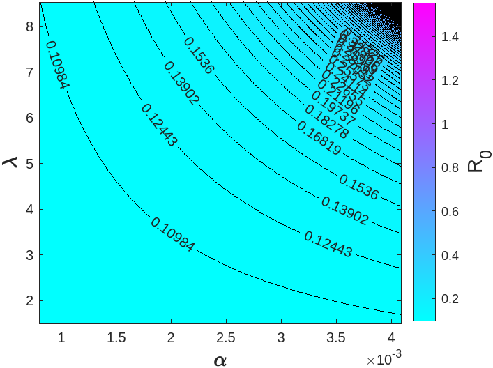
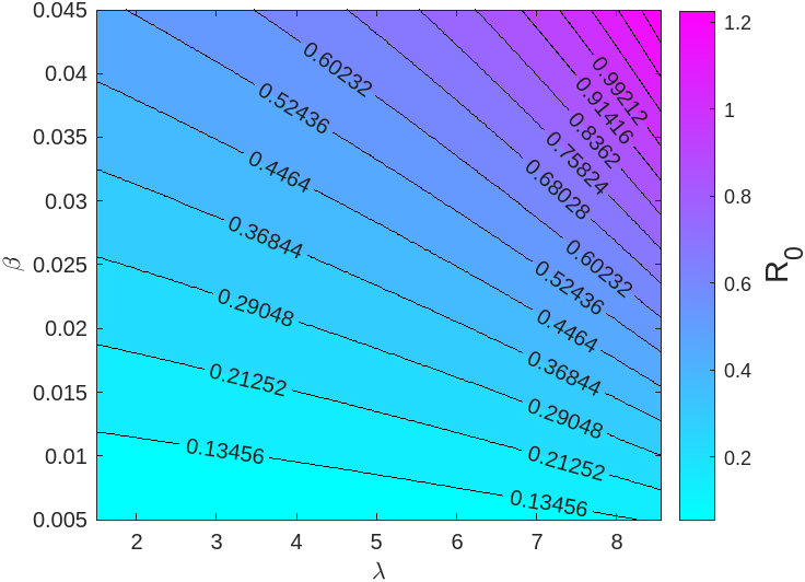
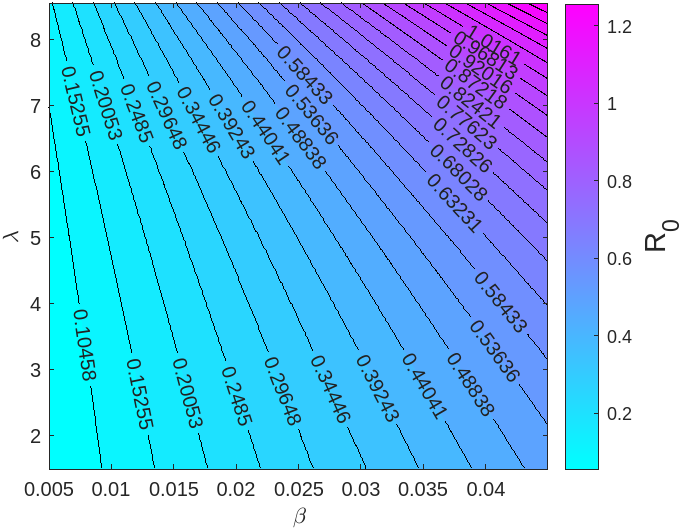
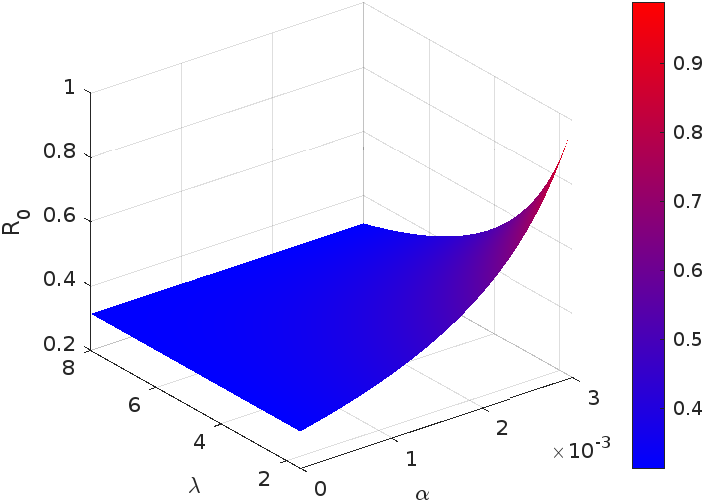
To understand how Hepatitis B might either die out or remain a long-term issue in a population, we used two different sets of parameters—Set A and Set B. Set A, with parameter set { $\lambda=6.56$ , $\alpha=0.003$ , $\beta=0.0095$ , $\gamma=0.42$ , $\delta=0.02$ , $\mu=0.0221$ , $\sigma=0.33$ , $\theta=0.012$ , $\tau=0.0026$ , r = 1.5, u = 0.39, b = 0.5}, was chosen to represent conditions that could lead to the extinction of the disease. Meanwhile, Set B, with parameter values { $\lambda=6.56$ , $\alpha=0.003$ , $\beta=0.0091$ , $\gamma=0.42$ , $\delta=0.02$ , $\mu=0.0121$ , $\sigma=0.33$ , $\theta=0.012$ , $\tau=0.0026$ , r = 0.09005, u = 0.19, b = 0.007}, reflects scenarios where the disease is more likely to persist in the community.

Both sets of parameters were simulated with the same initial population states: $(S(0),A(0),C(0),R(0))=(1000,320,50,10)$ , subjecting the process to run for 800 time units, using MATLAB’s ode45 solver. The results are illustrated in Fig. 6 and Fig. 7, which describe the temporal dynamics of the susceptible, acute, chronic, and recovered populations.

In Fig.6, the blue trajectories corresponding to Set A (where $R_{0}<1$ ), illustrate a consistent reduction in the infection. With time passing, the acute and chronic compartments reach zero, with the susceptible and recovered populations dominating in the long term. This direction is suggestive of effective disease eradication under the given conditions.

Conversely, the red trajectories, computed using Set B ( $R_{0}>1$ ), illustrate recurrent levels of acute and chronic infection over the long term, suggestive of the repeated occurrence of the disease. Here, every compartment, i.e., recovered, chronic, acute, and susceptible, has nonzero equilibrium values, reflecting the long-term presence of infected cases in the population.

Together, these findings point to a foundational epidemiological principle: if $R_{0}<1$ , the disease is fated for eventual eradication with a residual population of only recovered and susceptible members. If $R_{0}>1$ , the infection will persist, leaving behind a residual burden on the population in the form of both acute and chronic diseases.

We also examined the time-dependent reproduction number, $\mathcal{R}_{0}(t)$ , for each intervention strategy; see Fig. 7. When both vaccination and treatment controls were implemented in tandem, $\mathcal{R}_{0}(t)$ remained below the critical threshold of one for a significant portion of the time horizon. This is a promising outcome, indicating that such a strategy could feasibly lead to long-term control or even elimination of the virus.

8.2 Simulation of Optimal Control Analysis

We carry out numerical simulations of the proposed HBV model, both with and without the control strategies [2] to illustrate their impact. To obtain the solutions, we use the forward-backward sweep method, which is a standard numerical approach for solving optimal control problems. In this scheme, the state equations are solved forward in time using the control functions, and the adjoint equations are solved backward in time to update the co-state variables. The control values $u_{1}(t)$ and $u_{2}(t)$ are updated by minimizing the Hamiltonian at each time step. Optimal control is achieved when the control profile converges according to Pontryagin’s principle. The weight constants and balancing constants are considered as $k_{1}$ = 1, $k_{2}$ = 10, $w_{1}$ = 15, and $w_{2}$ = 5. In the following figures, the red dashed lines illustrate the dynamics of different population compartments under control measures, whilst the blue lines signify population behavior in the absence of interventions. We graphically show the influence and efficacy of the control measures proposed by different sets of strategies. By incorporating these two control variables, we investigated three strategies for eradicating HBV infection. The impact and efficacy of each strategy for eliminating the disease are depicted graphically.

Scenario 1: Use of Single Control Parameters

Strategy 1: Implementing Vaccination ( $u_{1}(t)$ ) Control Only

In this strategy, we use a single control parameter to curb the transmission of HBV and observe its effect on the population. So we use the control parameter $u_{1}(t)$ as an optimized parameter and $u_{2}(t)$ as an unoptimized parameter and compare the model dynamics when there is no control at all. In this situation, we observe a significant decrease in infections in both acute and chronic populations; see Fig. 8.

Strategy 2: Implementing Treatment ( $u_{2}(t)$ ) Control Only

In this strategy, we again use one control parameter to curb HBV transmission and observe the effect on the population. So we use the control parameter $u_{2}(t)$ as an optimized parameter and $u_{1}(t)$ as an unoptimized parameter and compare the model dynamics when there is no control at all. In this case, we observe a significant decrease in infections in both acute and chronic populations; see Fig. 9.

Scenario 2: Use of Coupled Control Parameters

Strategy 3: Implementing both Vaccination ( $u_{1}(t)$ ) & Treatment ( $u_{2}(t)$ ) Controls

In this strategy, we use two control parameters to control the transmission of HBV and see the influence on population dynamics. So we use the control parameters $u_{1}(t)$ and $u_{2}(t)$ both as optimized parameters and compare the model dynamics when there is no control at all. We get very good results in controlling infection in both acute and chronic populations, see Fig. 10.

Results and Discussion

Our findings underscore the substantial impact that optimal control measures can have on the spread of Hepatitis B. In the absence of any intervention, both acute and chronic infections remained consistently elevated throughout the simulation period. Introducing a control strategy focused solely on reducing susceptibility through $u_{1}(t)$ , representing vaccination, led to a noticeable reduction in the number of susceptible individuals, alongside a modest increase in the recovered population. This suggests that preventive strategies alone can begin to alter the trajectory of the epidemic.

In contrast, applying control exclusively to the chronically infected population via $u_{2}(t)$ , representing treatment, resulted in a more immediate decline in chronic infections. However, this approach had a limited effect on the susceptible and recovered groups, indicating a narrower but more targeted outcome. The most significant reduction in the overall disease burden was achieved by employing both control strategies simultaneously. Under this combined approach, the infected compartments declined sharply while the recovered population rose considerably, highlighting the importance of integrated prevention and treatment efforts.

During the early phase of the simulation, control efforts were applied with the greatest intensity, suggesting that prompt intervention is critical for limiting transmission. As infection levels declined over time, the optimal control inputs decreased gradually. This trend mirrors real-world public health strategies, where early and aggressive responses are essential to suppress outbreaks.

Additionally, as illustrated in Fig. 11, implementing either vaccination control $u_{1}(t)$ or treatment control $u_{2}(t)$ individually led to a notable decline in the infected population. But when we were implementing both the control measures simultaneously, the reduction in the infectious population was surprisingly very high, and the recovered population was greater than any other single intervention. Moreover, we observed reduced peak infection levels and a smaller final outbreak size across all compartments, reinforcing the effectiveness of a combined intervention approach.

9 Conclusion and Recommendations

In this work, we constructed and analyzed a mathematical model to study the transmission dynamics of Hepatitis B virus (HBV) infection, incorporating the roles of vaccination and treatment interventions. The model accounts for key epidemiological processes such as vertical transmission, chronic infection, and nonlinear treatment effects. Through rigorous analytical methods, we derived the basic reproduction number, $\mathcal{R}_{0}$ , and demonstrated that the disease-free equilibrium is both locally and globally asymptotically stable when $\mathcal{R}_{0}<1$ . Conversely, the infection persists when $\mathcal{R}_{0}>1$ , in line with expectations from classical epidemic theory [31].

A global sensitivity analysis employing Latin Hypercube Sampling (LHS) and Partial Rank Correlation Coefficients (PRCC) identified the transmission rates ( $\alpha$ & $\beta$ ) and the disease-induced death rate ( $\tau$ ) as the most impactful parameters influencing HBV prevalence. These findings suggest that effective strategies focused on reducing contact transmission and improving patient survival through timely treatment could substantially limit disease spread.

To evaluate the impact of intervention strategies, we applied Pontryagin’s Maximum Principle [23] and derived the optimality conditions for control measures involving vaccination and treatment. Numerical simulations confirmed that combining both controls is more effective than applying either strategy in isolation, significantly reducing the infected population and increasing recovery rates.

Recommendations

Based on the theoretical and computational results, we offer the following recommendations for HBV control and public health decision-making:

1.

Promote Integrated Vaccination and Treatment Campaigns
The model underscores the effectiveness of jointly administering vaccination and treatment. Policy frameworks should support programs that ensure coordinated delivery of both interventions, maximizing their synergistic effect.
2.

Reduce Contact Transmission in High-Risk Populations
Given the high sensitivity of the model to the contact rates $\alpha$ and $\beta$ , public health strategies should emphasize behavioral change, awareness campaigns, and targeted interventions in populations at increased risk of exposure [24].
3.

Expand and Sustain Vaccination Programs
The significant role of vaccination in lowering $\mathcal{R}_{0}$ justifies continued investment in expanding vaccine coverage, particularly in newborns and unvaccinated adults[1]. Immunization programs should include outreach components for hard-to-reach and vulnerable groups.
4.

Improve Access to Early Diagnosis and Treatment
To effectively reduce disease-induced mortality ( $\tau$ ) and enhance recovery, early diagnosis and equitable access to antiviral therapy must be prioritized, especially in settings with limited healthcare infrastructure [25].
5.

Incorporate Mathematical Modeling into Public Health Policy
This study illustrates the utility of optimal control and epidemiological modeling in informing the timing and allocation of interventions. Public health agencies are encouraged to integrate model-based tools into HBV elimination strategies[8].
6.

Invest in Surveillance and Model Refinement
Accurate and ongoing data collection is essential for calibrating models and assessing interventions. Enhancing health data infrastructure and supporting surveillance systems will facilitate more adaptive and responsive policymaking.

The current model forms a foundational structure that can be extended in future studies to include additional epidemiological complexities such as age stratification, co-infection dynamics, spatial heterogeneity, and behavioral changes. These extensions are essential to better inform policy and support long-term HBV elimination goals at national and global levels[31].

Authors contributions

All authors have contributed equally.

Data availability

This manuscript has no associated data.

Declarations

Conflict of interests

There is no conflict of interest regarding this work.

References

[1] S. A. Al-Busafi and A. Alwassief (2024) Global perspectives on the hepatitis b vaccination: challenges, achievements, and the road to elimination by 2030. Vaccines 12 (3), pp. 288. Cited by: item 3.
[2] H. Alrabaiah, M. A. Safi, M. H. DarAssi, B. Al-Hdaibat, S. Ullah, M. A. Khan, and S. A. A. Shah (2020) Optimal control analysis of hepatitis b virus with treatment and vaccination. Results in Physics 19, pp. 103599. Cited by: §8.1, §8.2.
[3] L. K. Beay and N. Anggriani (2022) Dynamical analysis of a modified epidemic model with saturated incidence rate and incomplete treatment. Axioms 11 (6), pp. 256. Cited by: §7, §8.1.
[4] C. Castillo-Chavez, S. Blower, P. van den Driessche, D. Kirschner, and A. Yakubu (2002) Mathematical approaches for emerging and reemerging infectious diseases: models, methods, and theory. Vol. 126, Springer Science & Business Media. Cited by: §6.2.1.
[5] C. Castillo-Chavez (2002) On the computation of r. and its role on global stability carlos castillo-chavez∗, zhilan feng, and wenzhang huang. Mathematical approaches for emerging and reemerging infectious diseases: an introduction 1, pp. 229. Cited by: §1, §6.2.1.
[6] O. Diekmann, J. A. P. Heesterbeek, and J. A. J. Metz (1990) On the definition and the computation of the basic reproduction ratio r 0 in models for infectious diseases in heterogeneous populations. Journal of mathematical biology 28, pp. 365–382. Cited by: §4.
[7] O. Diekmann and J. A. P. Heesterbeek (2000) Mathematical epidemiology of infectious diseases: model building, analysis and interpretation. Vol. 5, John Wiley & Sons. Cited by: §1, §4.
[8] P. J. Easterbrook, N. Luhmann, S. Bajis, M. S. Min, M. Newman, O. Lesi, and M. C. Doherty (2024) WHO 2024 hepatitis b guidelines: an opportunity to transform care. The lancet Gastroenterology & hepatology 9 (6), pp. 493–495. Cited by: item 5.
[9] J. K. Ghosh, U. Ghosh, M. Biswas, and S. Sarkar (2019) Qualitative analysis and optimal control strategy of an sir model with saturated incidence and treatment. Differential Equations and Dynamical Systems, pp. 1–15. Cited by: §1, §1, §7.
[10] A.B. Gumel and S.M. Moghadas (2003) A qualitative study of a vaccination model with non-linear incidence. Applied Mathematics and Computation 143 (2), pp. 409–419. External Links: ISSN 0096-3003, Document, Link Cited by: §1, §7.
[11] H. W. Hethcote (2000) The mathematics of infectious diseases. SIAM review 42 (4), pp. 599–653. Cited by: §1.
[12] A. Khan, R. Zarin, G. Hussain, A. H. Usman, U. W. Humphries, and J. Gomez-Aguilar (2021) Modeling and sensitivity analysis of hbv epidemic model with convex incidence rate. Results in Physics 22, pp. 103836. Cited by: §1.
[13] A. Khan, R. Zarin, M. Inc, G. Zaman, and B. Almohsen (2020) Stability analysis of leishmania epidemic model with harmonic mean type incidence rate. The European Physical Journal Plus 135 (6), pp. 528. Cited by: §1.
[14] T. Khan, G. Zaman, and M. I. Chohan (2017) The transmission dynamic and optimal control of acute and chronic hepatitis b. Journal of biological dynamics 11 (1), pp. 172–189. Cited by: §1, §1, §6.2.1, §7.
[15] T. Khan, G. Zaman, and A. Saleh Alshomrani (2018) Spreading dynamic of acute and carrier hepatitis b with nonlinear incidence. PloS one 13 (4), pp. e0191914. Cited by: §2.1.
[16] T. Khan and G. Zaman (2016) Classification of different hepatitis b infected individuals with saturated incidence rate. SpringerPlus 5 (1), pp. 1082. Cited by: §1.
[17] J. Li and Z. Ma (2002) Qualitative analyses of sis epidemic model with vaccination and varying total population size. Mathematical and Computer Modelling 35 (11-12), pp. 1235–1243. Cited by: §1.
[18] M. Y. Li and J. S. Muldowney (1995) Global stability for the seir model in epidemiology. Mathematical biosciences 125 (2), pp. 155–164. Cited by: §6.2.
[19] M. Y. Li and J. S. Muldowney (1996) A geometric approach to global-stability problems. SIAM Journal on Mathematical Analysis 27 (4), pp. 1070–1083. Cited by: §6.2.2, §6.2.2, §6.2.2.
[20] P. Liu, A. Din, and R. Zarin (2022) Numerical dynamics and fractional modeling of hepatitis b virus model with non-singular and non-local kernels. Results in Physics 39, pp. 105757. Cited by: §1.
[21] R. H. Martin Jr (1974) Logarithmic norms and projections applied to linear differential systems. Journal of Mathematical Analysis and Applications 45 (2), pp. 432–454. Cited by: §1.
[22] J. S. Muldowney (1990) Compound matrices and ordinary differential equations. The Rocky Mountain Journal of Mathematics, pp. 857–872. Cited by: §6.2.2.
[23] L.S. Pontryagin et al. (1962) The mathematical theory of optimal processes. Pergamon Press. Cited by: §9.
[24] C.W. Shepard, E.P. Simard, L. Finelli, et al. (2006) Hepatitis b virus infection: epidemiology and vaccination. Epidemiologic Reviews 28, pp. 112–125. Cited by: item 2.
[25] N.A. Terrault, A.S. Lok, B.J. McMahon, et al. (2018) Update on prevention, diagnosis, and treatment of chronic hepatitis b: aasld 2018 hepatitis b guidance. Hepatology 67 (4), pp. 1560–1599. Cited by: item 4.
[26] S. Thornley, C. Bullen, and M. Roberts (2008) Hepatitis b in a high prevalence new zealand population: a mathematical model applied to infection control policy. Journal of Theoretical Biology 254 (3), pp. 599–603. Cited by: §1.
[27] S. Umdekar, P. K. Sharma, and S. Sharma (2023) An seir model with modified saturated incidence rate and holling type ii treatment function. Computational and Mathematical Biophysics 11 (1), pp. 20220146. Cited by: §1.
[28] P. Van den Driessche and J. Watmough (2002) Reproduction numbers and sub-threshold endemic equilibria for compartmental models of disease transmission. Mathematical biosciences 180 (1-2), pp. 29–48. Cited by: §1, §4.
[29] W. Wang and S. Ruan (2004) Bifurcations in an epidemic model with constant removal rate of the infectives. Journal of Mathematical Analysis and Applications 291 (2), pp. 775–793. Cited by: §1.
[30] W. Wang (2006) Backward bifurcation of an epidemic model with treatment. Mathematical biosciences 201 (1-2), pp. 58–71. Cited by: §1.
[31] WHO (2024) Global hepatitis report 2024: action for access in low-and middle-income countries. World Health Organization Geneva, Switzerland. Cited by: §1, §9, §9.
[32] S. Yadav, A. S. Bhadauria, and V. S. Verma (2023) Study of an siqr model with optimal control techniques: a mathematical approach. Results in Control and Optimization 13, pp. 100327. Cited by: §5.
[33] G. Zaman, Y. H. Kang, and I. H. Jung (2008) Stability analysis and optimal vaccination of an sir epidemic model. BioSystems 93 (3), pp. 240–249. Cited by: §1, §7, §7, §7.
[34] R. Zarin, I. Ahmed, P. Kumam, A. Zeb, and A. Din (2021) Fractional modeling and optimal control analysis of rabies virus under the convex incidence rate. Results in Physics 28, pp. 104665. Cited by: §1.
[35] R. Zarin, A. Khan, M. Inc, U. W. Humphries, and T. Karite (2021) Dynamics of five grade leishmania epidemic model using fractional operator with mittag–leffler kernel. Chaos, Solitons & Fractals 147, pp. 110985. Cited by: §1, §1.
[36] X. Zhang and X. Liu (2008) Backward bifurcation of an epidemic model with saturated treatment function. Journal of mathematical analysis and applications 348 (1), pp. 433–443. Cited by: §1.
[37] L. Zou, W. Zhang, and S. Ruan (2010) Modeling the transmission dynamics and control of hepatitis b virus in china. Journal of theoretical biology 262 (2), pp. 330–338. Cited by: §1.

Analysis and Control of Hepatitis B Virus Spread with Harmonic Mean Incidence and Vertical Transmission: A Compartmental Modeling Approach

abstract

1 Introduction

2 Mathematical Model for the Dynamics of HBV Transmission

2.1 Positivity and Boundedness of Model

3 Disease Free Equilibrium Point (DFE)

4 Calculation of the Reproduction Number R0R_{0}

5 Existence of Endemic Equilibrium: Isocline Method

6 Stability Analysis of the Mathematical Model

6.1 Local Stability Analysis of HBV Mathematical Model

Theorem 1.

Proof.

Theorem 2.

Proof.

6.2 Global Stability Analysis of HBV Mathematical Model

6.2.1 Global Stability Analysis at Disease-Free Equilibrium

Theorem 3.

Proof.

Metzler Matrix BB

6.2.2 Global Stability Analysis at Endemic Equilibrium point

Theorem 4.

Proof.

7 Optimal Control Problem

8 Numerical Simulation for the Mathematical Model

8.1 Global Sensitivity Analysis

8.2 Simulation of Optimal Control Analysis

Scenario 1: Use of Single Control Parameters

Strategy 1: Implementing Vaccination (u1​(t)u_{1}(t)) Control Only

Strategy 2: Implementing Treatment (u2​(t)u_{2}(t)) Control Only

Scenario 2: Use of Coupled Control Parameters

Strategy 3: Implementing both Vaccination (u1​(t)u_{1}(t)) & Treatment (u2​(t)u_{2}(t)) Controls

Results and Discussion

9 Conclusion and Recommendations

Recommendations

Authors contributions

Data availability

Declarations

Conflict of interests

References

4 Calculation of the Reproduction Number $R_{0}$

Metzler Matrix $B$

Strategy 1: Implementing Vaccination ( $u_{1}(t)$ ) Control Only

Strategy 2: Implementing Treatment ( $u_{2}(t)$ ) Control Only

Strategy 3: Implementing both Vaccination ( $u_{1}(t)$ ) & Treatment ( $u_{2}(t)$ ) Controls