Programmable Doppler real-space pattern formation in cold atoms
Abstract
Red-detuned Doppler cooling decelerates atomic motion toward zero velocity, whereas blue-detuned light produces acceleration that separates a cold cloud into finite-velocity packets. Here we combine these complementary dynamics in a programmable split-stop protocol for real-space pattern formation. During each stage, a blue-detuned pulse splits existing packets and drives them apart, while a subsequent red-detuned pulse returns their center-of-mass velocities close to zero, results in spatially resolved stationary packets. Repeating this process recursively multiplies the number of packets in real space. We model the dynamics using stochastic photon-jump simulations that include absorption and spontaneous-emission recoil in one and two dimensions. Using experimentally realistic parameters for the transition of , we demonstrate an 8-packet one-dimensional array and a 64-packet two-dimensional square array.
I Introduction
A momentum-space crystal in cold atom is an atomic distribution in which the population occupies different velocity class, forming a discrete crystal like structure in momentum space. Its formation can be understood from the Doppler force produced by a pair of counter-propagating blue-detuned beams. For an atom moving along one beam, the co-propagating light is Doppler shifted towards resonance, whereas the counter-propagating light is shifted further from resonance. The resulting imbalance in the scattering rates accelerates the atom along its initial direction of motion. Consequently, an initially cold ensemble separates into two oppositely moving subclouds whose velocities become bunched around characteristic finite values. Therefore, the blue-detuned acceleration cause velocity bunching that generates discrete momentum packets arranged according to the geometry of the applied laser beams.
Momentum-space crystal in cold atom were first observed using narrow-line cooling of strontium 8; 7. In three-dimensional molasses, the momentum packets and spatial distributions resembling the lattice points of cubic or face-centered-cubic crystals, with their formations controlled by the detuning, saturation, and interaction time 7. Subsequent work revisited this phenomenon also in strontium samples 13. More recent experiments demonstrated momentum-space crystals in fermionic 87Sr and compared their formation on narrow- and broad-line transitions 4.
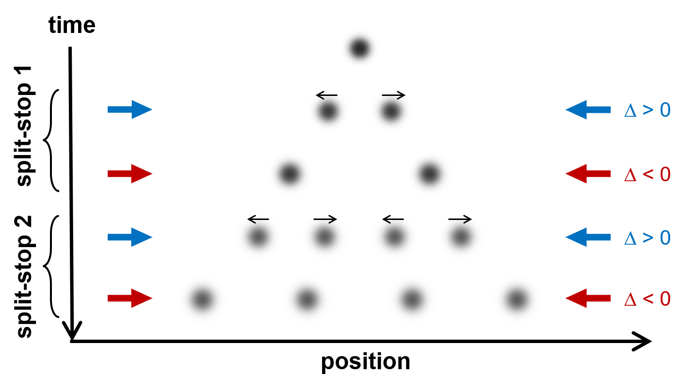
Building on this blue-detuned splitting mechanism, we introduce the split-stop protocol illustrated in Fig. 1. Starting from an initially cold atomic cloud, a blue-detuned pulse first divides the cloud into two oppositely moving subpackets. Rather than retaining these finite-velocity packets, a subsequent red-detuned pulse decelerates them and brings their center-of-mass velocities close to zero 2. The detuning is then returned to the blue side, causing each nearly stationary subpackets to split again, after which another red-detuned pulse stops the newly formed packets. Ideally, each split-stop cycle driven by one pair of counter-propagating beams doubles the number of spatially resolved packets along that axis. Each split-stop cycle drives an expansion and subsequent contraction of the packet distribution in momentum space, repeatedly returning the subpackets’ center of mass velocity close to zero without forming a persistent momentum-space crystal. Each such momentum-space “breath” multiplies the number of spatially separated subpackets, thereby constructing a progressively extended real-space pattern. By programming the pulse durations, detunings, and saturation parameters, we demonstrate the formation of extended one and two-dimensional cold-atom packet arrays.
II 1D Pattern Formation
II.1 model
We investigate the 1D atomic motion under counter-propagating laser beams. The scattering rate of a two-level atom experiencing a single beam traveling in (subscript with ) is given by
| (1) |
where is detuning-weighted saturation parameters
| (2) |
The sign is beam direction is the single-beam saturation parameter with being saturation intensity, is natural linewidth, is the detuning with being the time-dependent laser detuning and being the Doppler shift. To obtain eq.1 and 2, we employ an incoherent two-level rate-equation description inspired from literature 9; 12; 14. The counter-propagating beams are assumed to be mutually incoherent. The internal atomic state is assumed to follow the instantaneous optical steady state adiabatically. To simplify our study, the magnetic field and gravity effect are neglected.
The simulation is implemented using a stochastic photon-jump process. At each timestep , the total effective scattering rate is
| (3) |
For each atom, the number of complete scattering cycles occurring during that timestep is sampled from a Poisson distribution. Thus, a timestep may contain zero, one, or multiple scattering cycles. The timestep is chosen sufficiently small that the parameters and atomic dynamics changes are small. Each sampled scattering cycle consists of absorption from one of the two laser beams followed by spontaneous emission. Each effective scattering event is represented as a complete scattering cycle consisting of an absorption from one of the two laser beams followed by spontaneous emission. If a scattering event occurs, the probability that absorption is from beam is
| (4) |
A second uniformly distributed random number is therefore used to select the absorbing beam. Absorption from the beam gives the atom a momentum recoil whereas absorption from the beam gives .
The probabilities in Eq. (4) describe two limiting regimes: effective single-beam addressing and simultaneous two-beam addressing. At sufficiently large atomic velocities, the Doppler shift brings one beam much closer to resonance while shifting the counter-propagating beam further away from resonance. For example, when , one obtains , and the dynamics approach the single-beam-addressing limit. In contrast, near for two beams of equal intensity and detuning, and therefore , so that both beams contribute comparably to the atomic dynamics. Large saturation parameters broaden the detuning range over which and are comparable, allowing simultaneous two-beam addressing to happen over a wider range of atomic velocities.
Following the absorption recoil, the spontaneous-emission recoil is sampled independently. In the strictly one-dimensional recoil model, the atom receives a spontaneous-emission recoil of either or , each with probability . Since the absorption recoil is also , the total momentum change associated with a single effective scattering cycle can therefore take the values , , or .
We then evolve the trajectories of an ensemble of atoms to the target time, with the saturation parameter and detuning varied according to the designed pulse sequence.
II.2 Pattern formation
We first demonstrate the protocol by generating a finite one-dimensional array of eight spatially resolved atomic packets.
The laser protocol is specified by two time-dependent control parameters: the normalized detuning and the single-beam saturation parameter , which is identical for the two counterpropagating beams. Appropriate choices of these controls produce either blue-detuned packet splitting or red-detuned packet stopping. We construct the protocol from successive time segments with boundaries Within each segment, the parameters are linearly swept between start and end points of the segment. The endpoint values of adjacent segments need not coincide. For segment , we define the normalized local time
| (5) |
The complete control sequence is then
| (6a) | ||||
| (6b) | ||||
Here, and are the initial and final normalized detunings of segment , respectively, and is the saturation parameter of the pair of counterpropagating beam.
We initialize a one-dimensional ensemble of atoms with a Gaussian spatial distribution of width and a temperature of . These parameters are representative of experimentally demonstrated narrow-line red-MOT conditions for using the transition, which is also used throughout our simulations 11; 6. The atomic trajectories are propagated using a fixed timestep of .
h

As shown in Fig. 2, the protocol comprises three stages that successively increase the number of packets from , , and . Each stage consists of a blue-detuned splitting subsequence followed by a red-detuned stopping subsequence. Both subsequences employ a hold–ramp–hold structure: the detuning is first held constant, then swept linearly, and finally held at its terminal value. The saturation parameter remains constant within each subsequence but may change between the splitting and stopping subsequences and between successive stages.
At , the ensemble consists of a single Gaussian cloud. Stage 1 begins with a blue-detuned seed pulse at , which preferentially accelerates the slower atoms in opposite directions. As their Doppler shifts increase, the detuning is swept linearly to over , thereby tracking the accelerating atoms and driving the two subpackets to higher velocities. The detuning is then held at for . This terminal hold bunches the atoms around their final velocities while allowing the two subpackets additional time to separate spatially. The velocity separation is largest at the end of this blue-detuned hold, as shown by snapshot A in Fig. 2(b).
The stopping subsequence begins by jumping the detuning to , which is held for to address the rapidly moving atoms. The detuning is subsequently swept towards resonance, reaching after . This sweep follows the decreasing Doppler shift of the decelerating atoms and maintains the stopping force as their velocities approach zero. Because the packets are nearly stationary at the end of the ramp, only a short terminal hold is required. As illustrated by snapshot B, the velocity distribution is once again centred near zero, while two well-separated spatial subpackets have formed.
The same split-stop principle is applied in stages 2 and 3 to produce four and eight packets, respectively. The saturation parameters of the splitting and stopping subsequences are numerically optimized to maximize the contrast between neighboring packets while maintaining narrow packet widths. The later stages require longer sweeps and holds because the ensemble already spans several millimeters, so the oppositely moving groups must travel farther to become fully separated. At the end of the complete sequence, , the ensemble forms eight well-resolved spatial packets. The variance of the final velocity distribution corresponds to an effective one-dimensional kinetic temperature of approximately .
III 2D Pattern Formation
III.1 model
The two-dimensional model is a direct vector extension of the 1D model built above. We consider four laser beams propagating along . The two counter-propagating pairs may have independently programmed detunings and and single-beam saturation parameters and . For beam , we define
| (7) |
where for the beams and for the beams. Scattering rate from beam is
| (8) |
Total scattering rate is . At each timestep, the number of scattering cycles experienced by each atom is randomly sampled from a Poisson distribution with mean . For each cycle, the absorbing beam is selected with probability
| (9) |
and contributes an atomic momentum kick . Spontaneous emission is sampled isotropically in three dimensions by drawing uniformly from and uniformly from , giving
| (10) |
The in-plane momentum change for one scattering cycle is therefore
| (11) |
III.2 Pattern formation
We will present a demonstration the formation of an square array of 64 spatially resolved atomic packets.
We consider simultaneous addressing by the two counterpropagating beam pairs along and , with identical detuning and saturation parameters,
| (12) |
Both beam pairs are therefore governed by the same sequence parameterization introduced in eq. 5, 6a, and 6b.

During a blue-detuned splitting subsequence, the Doppler force amplifies atoms according to the initial signs of the velocity components. For example, an atom with preferentially scatters from the beam, further increasing , whereas an atom with is preferentially driven in the opposite direction. An analogous process occurs along . The initial ensemble consequently separates into four velocity groups associated with the quadrants
| (13) |
Although each scattering event involves absorption from only one of the four beams, the accumulation of many events transfers momentum along both axes and drives the four groups toward the diagonal directions.
The subsequent red-detuned subsequence reverses this to produce a standard molasses. Along each axis, atoms preferentially scatter from the beam opposing their motion, bringing the four velocity groups back toward , leaving four approximately stationary and spatially separated packets. Each complete split-stop stage therefore increases the number of stationary packets by a factor of four.
Applying this operation recursively produces the hierarchy
| (14) |
corresponding to , , , and finally spatial packets as shown in Fig.3. Similar to the 1D protocol, the saturation parameters of the blue-detuned splitting and red-detuned stopping subsequences are optimized numerically within the chosen experimental bounds to maximize packet separation and contrast while limiting packet broadening. At the end of the complete sequence, , the ensemble has an effective two-dimensional kinetic temperature of approximately .
An alternative strategy is to control the and beam pairs independently, producing the sequential hierarchy . This axis-by-axis protocol provides greater control over the pattern geometry at the cost of a longer formation time. In the example considered here, producing 64 packets requires , compared with for simultaneous control. Details of the axis-by-axis protocol are provided in Appendix.C.
IV Conclusion
We introduce a split-stop protocol for recursively multiplying spatially resolved cold-atom packets. Using a stochastic photon-jump model in one and two dimensions, we simulate experimentally realistic implementations on the transition of , demonstrating an eight-packet 1D array and a 64-packet 2D square array.
Several directions naturally follow from this work. First, alternative beam configurations and addressing sequences could generate a wider range of packet geometries. Although the resulting patterns are neither single-atom resolved nor held in confining potentials, this approach may provide a comparatively coarse and simple method for preparing structured atomic density distributions without spatially patterned light.5; 10; 1; 3. Second, optimal-control methods could be used to design nonlinear detuning and intensity profiles that reduce the total sequence duration while maximizing packet contrast and minimizing packet width. Finally, although our example uses the narrow transition of strontium, the protocol could be extended to other atomic species, such as Ytterbium.
Appendix A 1D sequence parameters
| Stage 1: | Stage 2: | Stage 3: | |||||||||||||||
|---|---|---|---|---|---|---|---|---|---|---|---|---|---|---|---|---|---|
| 1 | 0.0 | 0.4 | 0.8 | 0.8 | 8.8 | 7 | 10.5 | 12.2 | 1.9 | 1.9 | 10.7 | 13 | 26.3 | 27.7 | 1.7 | 1.7 | 4.5 |
| 2 | 0.4 | 2.9 | 0.8 | 11.3 | 8.8 | 8 | 12.2 | 15.2 | 1.9 | 19.9 | 10.7 | 14 | 27.7 | 38.1 | 1.7 | 29.9 | 4.5 |
| 3 | 2.9 | 5.5 | 11.3 | 11.3 | 8.8 | 9 | 15.2 | 16.7 | 19.9 | 19.9 | 10.7 | 15 | 38.1 | 40.1 | 29.9 | 29.9 | 4.5 |
| 4 | 5.5 | 6.0 | -25.3 | -25.3 | 12.5 | 10 | 16.7 | 17.0 | -35.5 | -35.5 | 7.2 | 16 | 40.1 | 41.1 | -39.6 | -39.6 | 8.2 |
| 5 | 6.0 | 10.4 | -25.3 | -1.2 | 12.5 | 11 | 17.0 | 26.1 | -35.5 | -3.0 | 7.2 | 17 | 41.1 | 51.3 | -39.6 | -2.9 | 8.2 |
| 6 | 10.4 | 10.5 | -1.2 | -1.2 | 12.5 | 12 | 26.1 | 26.3 | -3.0 | -3.0 | 7.2 | 18 | 51.3 | 51.5 | -2.9 | -2.9 | 8.2 |
Appendix B 2D sequence parameters
The control parameters used to generate Fig. 3 are listed in Table 2. The same controls are applied simultaneously to the counterpropagating beam pairs along and .
| Stage 1: | Stage 2: | Stage 3: | |||||||||||||||
|---|---|---|---|---|---|---|---|---|---|---|---|---|---|---|---|---|---|
| 1 | 0.0 | 0.5 | 0.8 | 0.8 | 8.8 | 7 | 13.6 | 15.8 | 1.9 | 1.9 | 10.7 | 13 | 34.2 | 36.0 | 1.7 | 1.7 | 4.5 |
| 2 | 0.5 | 3.7 | 0.8 | 11.3 | 8.8 | 8 | 15.8 | 19.7 | 1.9 | 19.9 | 10.7 | 14 | 36.0 | 49.5 | 1.7 | 29.9 | 4.5 |
| 3 | 3.7 | 7.1 | 11.3 | 11.3 | 8.8 | 9 | 19.7 | 21.7 | 19.9 | 19.9 | 10.7 | 15 | 49.5 | 52.1 | 29.9 | 29.9 | 4.5 |
| 4 | 7.1 | 7.8 | -25.3 | -25.3 | 12.5 | 10 | 21.7 | 22.1 | -35.5 | -35.5 | 7.2 | 16 | 52.1 | 53.4 | -39.6 | -39.6 | 8.2 |
| 5 | 7.8 | 13.5 | -25.3 | -1.2 | 12.5 | 11 | 22.1 | 33.9 | -35.5 | -3.0 | 7.2 | 17 | 53.4 | 66.7 | -39.6 | -2.9 | 8.2 |
| 6 | 13.5 | 13.6 | -1.2 | -1.2 | 12.5 | 12 | 33.9 | 34.2 | -3.0 | -3.0 | 7.2 | 18 | 66.7 | 67.0 | -2.9 | -2.9 | 8.2 |
Appendix C 2D axis-by-axis addressing
An alternative strategy is to address the and beam pairs sequentially, as illustrated in Fig. 4. During each split-stop operation, one beam pair actively divides the cloud along its axis, while the orthogonal pair is held at a red-detuned molasses that suppresses expansion in the other direction. Alternating the addressed axis therefore produces the hierarchy spatial packets. This axis-by-axis protocol provides independent control over the two directions and therefore offers greater flexibility in determining the pattern geometry. The trade-off is a longer sequence: each operation doubles the number of packets, whereas simultaneous addressing of both axes can increase the packet number by a factor of four in a single split-stop stage.

The axis-by-axis protocol uses the same piecewise-linear segment definitions in eq. 5–6b, but the two counterpropagating beam pairs are programmed independently. For each axis , we divide the complete protocol into contiguous segments with boundaries and define
The controls applied to beam pair are
| (15a) | ||||
| (15b) | ||||
The red-detuned periods are included explicitly as segments with and . The complete and sequences are listed in Tables 3 and 4, respectively.
| 1 | 0.0 | 0.4 | 0.8 | 0.8 | 8.8 | 8 | 23.2 | 25.1 | 1.9 | 1.9 | 10.7 | 15 | 58.0 | 59.5 | 1.7 | 1.7 | 4.5 |
|---|---|---|---|---|---|---|---|---|---|---|---|---|---|---|---|---|---|
| 2 | 0.4 | 3.2 | 0.8 | 11.3 | 8.8 | 9 | 25.1 | 28.4 | 1.9 | 19.9 | 10.7 | 16 | 59.5 | 70.9 | 1.7 | 29.9 | 4.5 |
| 3 | 3.2 | 6.1 | 11.3 | 11.3 | 8.8 | 10 | 28.4 | 30.1 | 19.9 | 19.9 | 10.7 | 17 | 70.9 | 73.1 | 29.9 | 29.9 | 4.5 |
| 4 | 6.1 | 6.7 | -25.3 | -25.3 | 12.5 | 11 | 30.1 | 30.4 | -35.5 | -35.5 | 7.2 | 18 | 73.1 | 74.2 | -39.6 | -39.6 | 8.2 |
| 5 | 6.7 | 11.5 | -25.3 | -1.2 | 12.5 | 12 | 30.4 | 40.4 | -35.5 | -3.0 | 7.2 | 19 | 74.2 | 85.4 | -39.6 | -2.9 | 8.2 |
| 6 | 11.5 | 11.6 | -1.2 | -1.2 | 12.5 | 13 | 40.4 | 40.6 | -3.0 | -3.0 | 7.2 | 20 | 85.4 | 85.6 | -2.9 | -2.9 | 8.2 |
| 7 | 11.6 | 23.2 | -4.0 | -4.0 | 1.5 | 14 | 40.6 | 58.0 | -4.0 | -4.0 | 1.5 | 21 | 85.6 | 113.2 | -4.0 | -4.0 | 1.5 |
| 1 | 0.0 | 11.6 | -4.0 | -4.0 | 1.5 | 8 | 23.2 | 40.6 | -4.0 | -4.0 | 1.5 | 15 | 58.0 | 85.6 | -4.0 | -4.0 | 1.5 |
|---|---|---|---|---|---|---|---|---|---|---|---|---|---|---|---|---|---|
| 2 | 11.6 | 12.0 | 0.8 | 0.8 | 8.8 | 9 | 40.6 | 42.5 | 1.9 | 1.9 | 10.7 | 16 | 85.6 | 87.1 | 1.7 | 1.7 | 4.5 |
| 3 | 12.0 | 14.8 | 0.8 | 11.3 | 8.8 | 10 | 42.5 | 45.8 | 1.9 | 19.9 | 10.7 | 17 | 87.1 | 98.5 | 1.7 | 29.9 | 4.5 |
| 4 | 14.8 | 17.7 | 11.3 | 11.3 | 8.8 | 11 | 45.8 | 47.5 | 19.9 | 19.9 | 10.7 | 18 | 98.5 | 100.7 | 29.9 | 29.9 | 4.5 |
| 5 | 17.7 | 18.3 | -25.3 | -25.3 | 12.5 | 12 | 47.5 | 47.8 | -35.5 | -35.5 | 7.2 | 19 | 100.7 | 101.8 | -39.6 | -39.6 | 8.2 |
| 6 | 18.3 | 23.1 | -25.3 | -1.2 | 12.5 | 13 | 47.8 | 57.8 | -35.5 | -3.0 | 7.2 | 20 | 101.8 | 113.0 | -39.6 | -2.9 | 8.2 |
| 7 | 23.1 | 23.2 | -1.2 | -1.2 | 12.5 | 14 | 57.8 | 58.0 | -3.0 | -3.0 | 7.2 | 21 | 113.0 | 113.2 | -2.9 | -2.9 | 8.2 |
References
- An atom-by-atom assembler of defect-free arbitrary two-dimensional atomic arrays. Science 354 (6315), pp. 1021–1023. External Links: Document Cited by: §IV.
- Three-dimensional viscous confinement and cooling of atoms by resonance radiation pressure. Phys. Rev. Lett. 55, pp. 48–51. External Links: Document Cited by: §I.
- Atom-by-atom assembly of defect-free one-dimensional cold atom arrays. Science 354 (6315), pp. 1024–1027. External Links: Document Cited by: §IV.
- Momentum-space crystal in narrow-line cooling of Sr. Chinese Physics B 28 (1), pp. 013701. External Links: Document Cited by: §I.
- Experimental demonstration of painting arbitrary and dynamic potentials for Bose–Einstein condensates. New Journal of Physics 11 (4), pp. 043030. External Links: Document Cited by: §IV.
- Magneto-optical trapping and cooling of strontium atoms down to the photon recoil temperature. Physical Review Letters 82 (6), pp. 1116–1119. External Links: Document Cited by: §II.2.
- Narrow line cooling and momentum-space crystals. Physical Review A 70 (6), pp. 063413. External Links: Document Cited by: §I.
- Narrow line cooling: finite photon recoil dynamics. Physical Review Letters 93 (7), pp. 073003. External Links: Document Cited by: §I.
- Resonance-radiation pressure on atoms in symmetrical light fields. Optics Letters 10 (4), pp. 179–181. External Links: Document Cited by: §II.1.
- Single-atom trapping in holographic 2D arrays of microtraps with arbitrary geometries. Physical Review X 4 (2), pp. 021034. External Links: Document Cited by: §IV.
- Progress toward ultra-cold Sr for the AION project—a red MOT and an optical-heterodyne diagnostic tool for injection-locked laser diodes. AVS Quantum Science 6 (1), pp. 014408. External Links: Document Cited by: §II.2.
- Radiation pressure on a two-level atom: an exact analytical approach. Journal of the Optical Society of America B 35 (1), pp. 127–132. External Links: Document Cited by: §II.1.
- Degenerate quantum gases of strontium. Ph.D. Thesis, University of Innsbruck, Innsbruck, Austria. External Links: Link Cited by: §I.
- A high-flux source of cold strontium with a loading rate of atoms/s for open release. AVS Quantum Science 8 (3), pp. 033201. External Links: Document Cited by: §II.1.