Extraction of DVCS amplitudes off the nucleon

The theory-agnostic model is constructed without any physical assumptions. It is utilized to independently extract the real and imaginary parts of the CFFs, relying solely on the statistical power of the experimental data. Such an agnostic method enables an unbiased extraction and was previously employed in Ref. 99 on a subset of the data analyzed in the current study.

The Ansätze for the real and imaginary parts of a generic CFF, $\mathcal{F}$, are parameterized by two independent ANNs, each featuring a single hidden layer composed of $n$ neurons. The input to each network is a 6-dimensional vector containing the scaled kinematic variables and their logarithmic transformations:

The scaling is introduced to improve training stability and performance. Specifically, the components are linearly scaled to approximately the range $(-1,1)$ before being fed into the network:

where $v\in\{\xi,\log_{10}\xi,|t|,\log_{10}|t|,Q^{2},\log_{10}Q^{2}\}$. The values of $v_{\mathrm{min}}$ and $v_{\mathrm{max}}$ are summarized in Table 1.

We utilize both linear kinematic variables and their logarithmic counterparts to accurately capture the dynamics of CFFs across both small and large values of $\xi$, $t$, and $Q^{2}$. For instance, capturing the small-$\xi$ behavior ($\xi<0.01$) would require an overly complex and flexible network if the inputs depended only linearly on this variable. Conversely, relying solely on a logarithmic transformation would present a similar problem in describing the large-$\xi$ behavior ($\xi>0.5$).

In matrix notation, the pre-scaled outputs of the networks are given by:

The matrices ${W}_{\mathrm{in}}\in\mathbb{R}^{n\times 6}$ and ${W}_{\mathrm{out}}\in\mathbb{R}^{1\times n}$ denote the weights of the hidden (inner) and output layers, respectively, while $\vec{b}_{\mathrm{in}}\in\mathbb{R}^{n}$ and $b_{\mathrm{out}}\in\mathbb{R}$ denote the corresponding biases. The activation function applied element-wise within the hidden layer is the sigmoid linear unit (SiLU), defined as:

which is depicted in Fig. 2.

A linear scaling is applied to the final output of the network. Assuming the normalized network yields a value roughly within $(-1,1)$, it is mapped back to the physical output domain of the CFF multiplied by $\xi$, $(O_{\mathrm{min}},O_{\mathrm{max}})=(-5,5)$:

The free parameters of the Ansatz, namely, the weights and biases, are optimized during the training phase, as detailed in Sect. 4.7. Prior to training, the weights are randomly initialized from a normal distribution $\mathcal{N}(\mu=0,\sigma=2.5)$ to break the initial symmetry between the nodes. Simultaneously, the biases are initialized to zero to ensure the initial pre-activations remain zero-centered, preventing premature saturation. Together, these choices enable stable and effective gradient-based optimization.

In the case of the theory-augmented model, we impose the following theory-driven constraints:

• •

  dispersion relations: exploiting dispersion relations eliminates the need to independently parameterize the real and imaginary parts of the CFFs $\mathcal{H}^{++}$, $\mathcal{E}^{++}$, $\widetilde{\mathcal{H}}^{++}$, and $\widetilde{\mathcal{E}}^{++}$ (which would otherwise require eight 3D functions). Instead, it suffices to model the imaginary parts and a single subtraction constant, reducing the problem to four 3D functions and one 2D function. Because the dispersion relations for the remaining two CFFs ($\mathcal{H}^{+-}$ and $\mathcal{H}^{0+}$) are currently unknown, we constrain their real and imaginary parts separately.

Furthermore, we impose several additional constraints guided by the standard modeling of GPDs, their connections to PDFs and EFFs, and their ultimate impact on CFFs:

• •

  the imaginary parts of the CFFs receive distinct contributions from valence quarks, sea quarks, and gluons. These contributions are characterized by the power-law form $\xi^{\alpha}(1-\xi)^{\beta}$, which vanishes at $\xi=1$ and may exhibit a singularity as $\xi\to 0$. The exponent $\alpha$ differs significantly between the valence and sea/gluon sectors, yielding distinct $\xi$-dependent profiles for each contribution to the CFFs.

• •

  kinematic dependencies on both $Q^{2}$ and $t$ are introduced into the exponent $\alpha$, reflecting the evolution of the PDFs and the Regge behaviour, respectively.

• •

  an dipole-like falloff with respect to $-t$ is enforced, mirroring the well-established relationship between GPDs and EFFs for the nucleon.

These physical considerations motivate the following Ansatz for the pre-scaled imaginary parts of the CFFs:

where $\Lambda_{\mathrm{Im}}$ is fitted to the data, and

with $Q^{2}_{0}=2\,\mathrm{GeV}^{2}$.

We employ $n_{\mathrm{net}}=2$ independent networks to describe the residual shape of the CFFs beyond the assumed power-law forms, which roughly correspond to the valence and sea/gluon sectors. Our Ansatz is scalable, allowing a higher value for $n_{\mathrm{net}}$ to be adopted if required by the data.

The inputs to the networks are two-dimensional vectors,

whose elements rely on the previously defined scaling transformations using the parameters summarized in Table 1. Unlike in the theory-agnostic model, we do not use both linear and logarithmic variables. This is because the present model is inherently constrained at the endpoints. In particular, the imaginary parts of the CFFs vanish identically as $\xi\to 1$.

In matrix notation, the ANNs are defined by the following equations:

Here, for simplicity, we assume that each network consists of the same number of hidden neurons, $n$. For the shape networks ($k\in\{1,\dots,n_{\mathrm{net}}\}$), the matrices $W^{(\mathrm{Im},k)}_{\mathrm{in}}\in\mathbb{R}^{n\times 2}$ and $W^{(\mathrm{Im},k)}_{\mathrm{out}}\in\mathbb{R}^{1\times n}$ denote the weights of the hidden and output layers, respectively, with $\vec{b}^{(\mathrm{Im},k)}_{\mathrm{in}}\in\mathbb{R}^{n}$ and $b^{(\mathrm{Im},k)}_{\mathrm{out}}\in\mathbb{R}$ representing the corresponding biases. Similarly, the parameters for the network related to the $t$-dependence are given by $W^{(\mathrm{Im},t)}_{\mathrm{in}}\in\mathbb{R}^{n\times 2}$, $W^{(\mathrm{Im},t)}_{\mathrm{out}}\in\mathbb{R}^{1\times n}$, $\vec{b}^{(\mathrm{Im},t)}_{\mathrm{in}}\in\mathbb{R}^{n}$, and $b^{(\mathrm{Im},t)}_{\mathrm{out}}\in\mathbb{R}$.

While the shape networks utilize the SiLU activation function, the network used to describe the $t$-dependence employs a sigmoid activation function:

This choice provides a more stable training environment by naturally bounding the output to the $(0,1)$ range (see Fig. 2). Constraining the outer biases $b^{(\mathrm{Im},t)}_{\mathrm{out}}$ and weights $W^{(\mathrm{Im},t)}_{\mathrm{out}}$ to be strictly positive guarantees that the Ansatz does not diverge as $-t\to\infty$. The linear output scaling used to map $\overline{O}^{(\mathrm{Im})}$ back to the physical domain remains identical to that of the theory-agnostic model, see Eq. (21).

The real parts of the CFFs $\mathcal{H}^{+-}$ and $\mathcal{H}^{0+}$ are parameterized exactly like the imaginary parts, with the exception of setting the exponents $\beta_{k}=0$. This removes the requirement for the functions to vanish at $\xi=1$. Unlike the imaginary parts, which are kinematically restricted to vanish at this boundary in the direct channel, the real parts are not bound by this restriction due to their analytic continuation into crossed channels (see for instance Ref. 108).

Finally, the subtraction constant, which depends exclusively on $t$ and $Q^{2}$, is parameterized as the product of a $Q^{2}$-dependent parameter describing the magnitude at $t=0$ and, as previously, a dipole-like structure describing the falloff in $-t$:

The neural network $\mathrm{ANN}^{(\mathrm{SC},t)}(x_{\mathrm{1D}})$ takes only the scaled logarithmic $Q^{2}$ variable as input,

and in matrix notation it is defined by the following equation:

Here, $n$ again represents the number of hidden neurons. The matrices $W^{(\mathrm{SC},t)}_{\mathrm{in}}\in\mathbb{R}^{n\times 1}$ and $W^{(\mathrm{SC},t)}_{\mathrm{out}}\in\mathbb{R}^{1\times n}$ denote the weights of the hidden and output layers, respectively, with $\vec{b}^{(\mathrm{SC},t)}_{\mathrm{in}}\in\mathbb{R}^{n}$ and $b^{(\mathrm{SC},t)}_{\mathrm{out}}\in\mathbb{R}$ representing the corresponding biases.

The magnitude at $t=0$ explicitly mimics the $Q^{2}$ evolution and is defined as:

where $\Lambda_{\mathrm{QCD}}=0.2\,\mathrm{GeV}$ is the QCD scale parameter, $Q_{0}^{2}=2\,\mathrm{GeV}^{2}$ is the reference scale, and $p_{i}$ are free parameters controlling the effective $Q^{2}$ evolution.

Prior to the optimization phase, all free parameters of the theory-augmented Ansatz are initialized using specific statistical distributions. The baseline powers governing the dominant power-law behaviour are initialized from uniform distributions, with $\alpha_{1,0}\sim\mathcal{U}(a=0,b=0.5)$ for the first network term, $\alpha_{2,0}\sim\mathcal{U}(-0.5,0)$ for the second, and $\beta_{k}\sim\mathcal{N}(0.5,0.1)$ for both $k\in\{1,2\}$. Determining appropriate initial values for $\beta_{k}$ poses a challenge because excessively high values force the distributions to vanish too rapidly as $\xi\to 1$, affecting the uncertainty estimation in that region. The remaining parameters dictating the kinematic evolution of the baseline powers ($\alpha_{k,t}$ and $\alpha_{k,Q^{2}}$) are drawn from a narrow normal distribution, $\mathcal{N}(0,0.1)$, to introduce small initial perturbations centered around zero. The mass scale parameter $\Lambda_{\mathrm{Im}}^{2}$ is initialized from $\mathcal{N}(1,0.1)$.

For the neural networks describing the residual shape of the CFFs ($\mathrm{ANN}^{(\mathrm{Im},k)}$ with $k\in\{1,2\}$), the weights $W^{(\mathrm{Im},k)}_{\mathrm{in}}$ and $W^{(\mathrm{Im},k)}_{\mathrm{out}}$ are drawn from $\mathcal{N}(0,0.5)$, while their global output biases are initialized from a standard normal distribution as $b^{(\mathrm{Im},k)}_{\mathrm{out}}\sim\mathcal{N}(0,1)$. To model the global $t$-dependence and mimic standard dipole/tripole behaviour, the weights $W^{(\mathrm{Im},t)}_{\mathrm{in}}$ and $W^{(\mathrm{Im},t)}_{\mathrm{out}}$ of $\mathrm{ANN}^{(\mathrm{Im},t)}$ are initialized from $\mathcal{N}(0,0.5)$, with its global output bias drawn as $b^{(\mathrm{Im},t)}_{\mathrm{out}}\sim\mathcal{N}(3,0.1)$. To break symmetry without introducing unnecessary early saturation, the inner biases ($\vec{b}^{(\mathrm{Im},k)}_{\mathrm{in}}$ and $\vec{b}^{(\mathrm{Im},t)}_{\mathrm{in}}$) for the hidden neurons in all three networks are strictly initialized to zero.

Finally, the coefficients defining the subtraction constant are initialized according to distinct distributions to reflect their physical roles. The constant amplitude parameter $\mathcal{S}_{0}$ and the amplitude weights $\mathcal{S}_{i}$ are drawn from a uniform distribution, $\mathcal{U}(-10,10)$. To strictly ensure an asymptotically vanishing behaviour at high $Q^{2}$, the parameters $p_{i}$ are forced to be negative and are initialized from a uniform distribution $\mathcal{U}(-5,-1)$. The subtraction constant’s mass scale parameter $\Lambda_{\mathrm{SC}}^{2}$ is drawn from $\mathcal{N}(1,0.1)$. Analogous to the imaginary part, the $t$-dependence network $\mathrm{ANN}^{(\mathrm{SC},t)}$ for the subtraction constant has its weights $W^{(\mathrm{SC},t)}_{\mathrm{in}}$ and $W^{(\mathrm{SC},t)}_{\mathrm{out}}$ initialized from $\mathcal{N}(0,0.5)$, its inner biases $\vec{b}^{(\mathrm{SC},t)}_{\mathrm{in}}$ strictly set to zero, and its global output bias $b^{(\mathrm{SC},t)}_{\mathrm{out}}$ initialized from $\mathcal{N}(3,0.1)$.

Uncertainties are propagated from the experimental data using the standard replication method. Specifically, we perform the fit $101$ times. The first fit, referred to as “the central replica”, is performed on the original, unmodified data to obtain the central values of the model parameters. The remaining $100$ fits (replicas) are then performed on artificially fluctuated pseudodata. For the $i$-th replica, the value of the $j$-th point belonging to dataset $k$ is generated according to:

Here, $v_{j/k}$, $\sigma_{\mathrm{stat},j/k}$, $\sigma_{\mathrm{sys},j/k}$, and $\sigma_{\mathrm{norm},j/k}$ represent the central value, statistical uncertainty, systematic uncertainty, and normalization uncertainty of a given experimental point, respectively. The normalization uncertainty is typically associated with luminosity or polarization measurements.

The terms $\smash{\mathcal{N}^{(i)}_{j/k}(0,1)}$ and $\smash{\mathcal{N}^{(i)}_{k}(0,1)}$ denote random numbers drawn from a standard normal distribution. Crucially, $\smash{\mathcal{N}^{(i)}_{j/k}}$ is sampled independently for every single point, while $\smash{\mathcal{N}^{(i)}_{k}}$ is sampled only once per dataset for a given replica. This ensures that all points within a specific dataset shift coherently in response to the normalization uncertainty, correctly capturing its fully correlated nature. We treat the remaining systematic uncertainties as uncorrelated point-to-point, as the experimental publications generally do not provide sufficient covariance information to model them otherwise. Consequently, the total uncertainty associated with a given point, which enters the evaluation of $\chi^{2}_{\mathrm{data}}(\theta_{i})$ (see Eq. (36)), is given by:

where we explicitly expose the index $k$ associated with the dataset.

In the presented plots, the uncertainty bands represent the $68\%$ confidence interval. These bands are evaluated from the ensemble of $100$ replicas (excluding the central replica) using the quantile method, specifically by determining the interval bounded by the $16$th and $84$th percentiles.

In the global analysis of DVCS, the available experimental data are distributed highly unevenly across the kinematic phase space. Specifically, the low-$\xi$ regime covered by HERA is sparse compared to regions with higher $\xi$ covered by JLAB, which are densely populated by high-precision points. Additionally, the data overwhelmingly populate low $Q^{2}$ regions compared to high $Q^{2}$ ones. Standard optimization routines that minimize an unweighted $\chi^{2}$ loss function inherently prioritize regions with the highest data density. Consequently, the fit may fail to adequately capture the functional behaviour in sparse regions, treating them as statistically insignificant.

To mitigate this and ensure that sparse data, particularly at small $\xi$, remain “visible” during the optimization phase, we employ an inverse density weighting procedure. The procedure is executed over a two-dimensional grid spanning the kinematic variables $\xi$ and $Q^{2}$. Specifically, the phase space is discretized using uniform linear bins for both variables. The variable $\xi$ is partitioned into $200$ bins spanning the range $0<\xi<1$, while $Q^{2}$ is divided into $36$ bins covering the interval $1~\mathrm{GeV}^{2}<Q^{2}<10~\mathrm{GeV}^{2}$.

To evaluate the weights for the $N_{\mathrm{data}}$ experimental points used in the extraction, we first map them onto the aforementioned grid. Next, we define the “raw” weight for the $j$-th data point falling into the $i$-th bin as:

where $N_{\mathrm{unique},i}$ is the number of strictly unique $(\xi,Q^{2})$ coordinate pairs registered in the $i$-th bin (note that many experimental points may be characterised by the same values of $\xi$ and $Q^{2}$). The final, normalized weight $w_{j}$ assigned to the $j$-th data point is then calculated as:

By ensuring that $\sum_{j}w_{j}=N_{\mathrm{data}}$, the weighting procedure preserves the standard statistical interpretation of the loss function.

Note that in the limit of infinitely many bins (or infinitesimal bin sizes), each populated bin isolates exactly one unique kinematic setting, meaning $N_{\mathrm{unique},i}=1$ for all populated bins. In this limit, every data point receives a raw weight of $1$, and the procedure naturally and strictly recovers the standard unweighted scenario where $w_{j}=1$. This behaviour demonstrates that by changing the binning resolution, we can seamlessly control the strength of the $(\xi,Q^{2})$ density reweighting. The distribution of weights used in the current analysis is shown in Fig. 3.

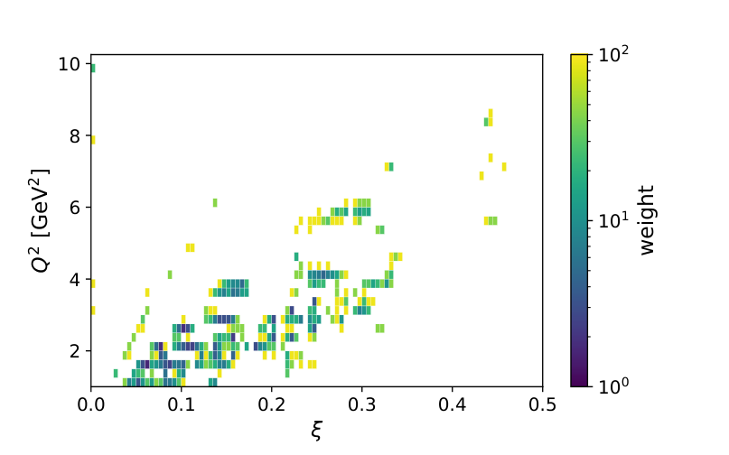
During the minimization procedure, the weights are incorporated into the goodness-of-fit function as follows:

Here, $\theta_{i}$ denotes a complete set of trainable parameters for the $i$-th replica, $v_{j}(\theta_{i})$ denotes the model predictions, while the $N_{\mathrm{data}}$ experimental data points are characterized by their measured values $v^{(\mathrm{exp})}_{j}$ and associated uncertainties $\sigma^{(\mathrm{exp})}_{j}$. In the following, we will also use the unweighted estimator, simply defined as:

The weighting procedure introduces an increase in $\chi^{2}_{\mathrm{data},\mathrm{uw}}$ of approximately $1\%$ compared to a fully unweighted extraction. The effect of this procedure is demonstrated in Fig. 4. For the theory-agnostic model, the impact is moderate, as expected. We primarily observe a reduction in the artificially inflated uncertainties associated with the unweighted extraction, an issue that could otherwise only be mitigated by using an unrealistically long training cycle and large networks. For the theory-augmented model, however, the effect is striking: the weighting procedure successfully prevents both bias and the inflation of uncertainties. It is also worth noting that the results for both models are in better agreement when the weighting procedure is used.

A fundamental challenge in employing artificial neural networks is managing the bias-variance trade-off. Due to their immense structural flexibility, ANNs inherently exhibit low bias but suffer from high variance, making them highly susceptible to overfitting the experimental data and capturing statistical noise. While traditional regularization techniques, such as standard L1 and L2 weight decay, effectively reduce variance by penalizing the magnitude of the network weights, they indiscriminately pull all parameters toward zero, resulting in underestimated and therefore unreliable uncertainties in domains not covered by data.

To systematically address this, we employ a technique known as anchored ensembling. Instead of penalizing the absolute magnitude of the trainable weights, we penalize their deviation from a set of fixed, randomly initialized anchor values. For each replica, we instantiate a set of corresponding prior networks alongside the trainable networks, keeping the parameters of these prior networks frozen. The total loss function optimized during the training of the $i$-th replica is thus modified to include an anchoring penalty:

where the data term, $\chi^{2}_{\mathrm{data}}(\theta_{i})$, was defined in Eq. (36). The anchoring penalty is defined as

Here, $\theta_{i}$ denotes the complete set of $N_{\mathrm{par}}$ trainable parameters for the model, $\theta^{(\mathrm{prior})}_{i}$ represents the fixed parameters of the random prior, and $\lambda$ is a hyperparameter that controls the strength of the regularization.

In summary, by assigning a distinct random prior anchor to each replica, the individual networks are encouraged to explore different regions of the loss landscape, ensuring a diverse ensemble. In kinematic regions that are well constrained by experimental data, the data term dominates the optimization and the dependence on the particular anchor becomes weak, leading the replicas to converge toward similar solutions. In sparsely populated regions, on the other hand, the anchoring term prevents the ensemble from collapsing onto a single arbitrary extrapolation, allowing the spread among replicas to reflect the reduced constraining power of the data.

Implementing the presented framework requires a strict, sequential tuning procedure to prevent hyperparameter coupling. To achieve this, we first fix the intrinsic capacity of the models by tuning the number of hidden neurons, ensuring that the networks possess sufficient flexibility to describe the underlying physics. After the network topology is established, we tune the anchoring hyperparameter, $\lambda$, to properly scale the ensemble variance relative to the experimental data.

Because directly fitting the model to experimental data is computationally expensive, we tune the hyperparameters using a generated set of CFF pseudodata. This pseudodata is constructed through the following procedure:

1. 1.

   for each kinematic point $(\xi,t,Q^{2})$ in the experimental dataset, we perform a local extraction (see, e.g., Ref. 57) to determine the CFFs and their associated uncertainties.

2. 2.

   for these same kinematic points, we compute the corresponding CFF values using the GK model and leading-order (LO) coefficient functions.

3. 3.

   we then smear these GK model CFFs according to the uncertainties obtained in the first step.

We utilize the GK model predictions, rather than the locally extracted central values, because local extraction is unreliable for datasets lacking an explicit $\phi$ dependence, such as the HERMES and HERA data. In such cases, estimating the correlations between the extracted CFFs is exceedingly challenging. Furthermore, since many observables are primarily sensitive to the square of the CFFs, the signs of the locally extracted CFFs remain largely unconstrained and can be entirely random.

We begin by determining the optimal number of hidden neurons. At this stage, we set the anchoring hyperparameter to $\lambda=0$, thereby disabling the influence of the prior distributions. Our goal is to identify the minimum number of neurons required to prevent the model from being too rigid to accurately describe the data. Conversely, we want to avoid excessive flexibility: overly complex models not only become computationally expensive but also require significantly heavier regularization to prevent overfitting, which can introduce unwanted numerical noise.

The dependence of the post-training loss $\chi^{2}_{\mathrm{data},\mathrm{uw}}(\theta_{0})$ on the number of neurons is illustrated in Fig. 5 for both models. For simplicity, in the theory-augmented case, we use the same number of neurons across all constituent networks, as well as an identical number of terms in the subtraction constant ansatz. For instance, $n=5$ indicates five hidden neurons in $\mathrm{ANN}^{(\mathrm{Im},k)}(\vec{x}_{\mathrm{2D}})$, where $k=1,2$, and $\mathrm{ANN}^{(\mathrm{Im},t)}(\vec{x}_{\mathrm{2D}})$, alongside five terms in the sum displayed in Eq. (31). As shown in the figure, insufficient network capacity restricts the model’s ability to accurately describe the data, manifesting as a systematic bias. In the theory-agnostic case, however, highly complex models suffer from overfitting. Consequently, we set $n=10$ for the theory-agnostic model and $n=5$ for the theory-augmented model.

Having determined the optimal network capacities, a process that inherently involves a degree of arbitrariness, we proceed to tune the anchoring hyperparameter $\lambda$. Figure 5 illustrates the dependence of the post-training loss $\chi^{2}_{\mathrm{data},\mathrm{uw}}(\theta_{0})$ on $\lambda$ for both architectures. As expected, if $\lambda$ is set too large, the optimization is dominated by the regularization penalty, driving the model too strongly toward the random prior and reintroducing a systematic bias. To balance this trade-off, ensuring ensemble diversity without sacrificing fit quality, we set $\lambda=0.01$ for the theory-agnostic model and $\lambda=0.1$ for the theory-augmented model.

The minimisation utilizes the Adam algorithm 86. To mitigate the computational and temporal costs of the minimization process, we accelerate convergence using a three-stage procedure (a technique known as warm-starting):

1. 1.

   first, we initialize a fully unconstrained model. The weights, biases, and any additional parameters (such as powers in the theory-augmented model) are randomly selected, as detailed in Secs. 4.1 and 4.2 introducing the models.

2. 2.

   second, using this unconstrained model, we perform a preliminary fit to pseudodata for the CFFs based on the GK model (these are the same pseudodata used to fix the hyperparameters, see Sect. 4.5). The rapid fit is terminated once $\chi^{2}_{\mathrm{data}}(\theta_{0})<25$ (with the very last iteration being discarded), ensuring that our initial ensemble of replicas forms a broad band around the CFFs predicted by the GK model.

3. 3.

   finally, using the parameters obtained from this intermediate step, we resume the fitting process, this time utilizing the actual experimental data.

This procedure is illustrated in Fig. 6, which displays the results for the fully unconstrained model, the model constrained by the preliminary fit to pseudo-data, and the final model constrained by the experimental data. Had we fitted the experimental data directly from a fully unconstrained model (i.e., omitting the intermediate step), the initial goodness-of-fit value would be on the order of $\chi^{2}_{\mathrm{data}}(\theta_{0})\sim 10^{7}$, significantly prolonging convergence. Instead, our intermediate step reduces the starting point for the final fit to approximately $\chi^{2}_{\mathrm{data}}(\theta_{0})\sim 10^{3}$.

Only for the theory-augmented model, the prefit procedure encounters difficulties at large $\xi$ due to a strong non-linear dependence of CFFs on the powers $\beta_{k}$ in the term $(1-x)^{\beta_{k}}$. Specifically, to ensure a broad uncertainty band as $\xi\to 1$, the values of $\beta_{k}$ must be small. Although they are initialized appropriately, the gradient-based training algorithm used in the prefit tends to increase these parameters on average due to the scarcity of data at large $\xi$. This artificial behaviour, however, does not impact the final extraction.

The minimization algorithm employs a batching strategy and is initialized with a learning rate of $0.05$. To dynamically refine the optimization, this rate is halved if the fit fails to improve for $20$ consecutive iterations. Additionally, we set the optimizer hyperparameters to $\beta_{1}=0.9$ and $\beta_{2}=0.9$, which dictate the exponential decay rates for the first and second moment estimates (tracking the moving averages of the gradient and the squared gradient, respectively). This specific configuration ensures stable and rapid convergence. The typical evolution of the losses $\chi^{2}_{\mathrm{data}}(\theta_{0})$ and $\chi^{2}_{\mathrm{data},\mathrm{uw}}(\theta_{0})$ as a function of the training epoch during the fit to experimental data is shown in Fig. 7 for both models.

In this analysis, we extract DVCS CFFs from experimental data separately for proton and neutron targets. A meaningful joint extraction for both targets can only be performed at the GPD level, unless one employs a more involved parameterization of CFFs that incorporates flavour separation, an approach inherently more susceptible to model dependencies. For a similar reason, we do not include the existing TCS data 38 in the current fit. Including these data would necessitate adopting specific relations between the DVCS and TCS amplitudes, thereby forcing us to perform the extraction at a fixed perturbative order in $\alpha_{s}$. Nevertheless, a comparison with the existing TCS data is presented at the end of this section.

For the fitting procedure, we restrict our analysis to data that satisfy the following kinematic cuts:

These kinematic criteria are modified with respect to our previous works and those by other phenomenology groups (see, for instance, Refs. 90). Namely, compared to Refs. 99, we relaxed the cuts from $Q^{2}>1.5~\mathrm{GeV}^{2}$ and $-t/Q^{2}<0.2$. In doing so, we have made the extraction more sensitive to both genuine and kinematic higher-twist effects. This approach is reasonable because, in this analysis, we explicitly include the kinematically suppressed helicity-flip $\mathcal{H}^{0+}$ and $\mathcal{H}^{+-}$ amplitudes, and we aim to match the extraction to the precision of the current understanding of DVCS in the language of GPDs 27.

The DVCS data considered in this study are summarized in Table 2 for both proton and neutron targets. This table also specifies the number of data points that passed the imposed kinematic cuts, as well as the post-fit $\chi^{2}_{\mathrm{data},\mathrm{uw}}(\theta_{0})$ values obtained for the central replicas of both models. For the proton target, the total $\chi^{2}_{\mathrm{data},\mathrm{uw}}(\theta_{0})$ is $1.29$ for the theory-agnostic model and $1.36$ for the theory-augmented model. The corresponding values for the neutron target are $0.76$ and $0.70$. For datasets common to both the present and our previous analysis 99, the resulting goodness-of-fit values are in good agreement. However, for the newly included data, particularly those from Ref. 79; 43, we generally observe higher $\chi^{2}_{\mathrm{data},\mathrm{uw}}(\theta_{0})$ values. Given that the theory-agnostic model minimises the risk of an inadequate Ansatz, this discrepancy points to either the presence of neglected theoretical contributions or residual systematic issues within the data themselves.

A collection of plots comparing our fit results with the experimental data is presented in Figs. 8 and 9 for the proton and neutron targets, respectively. In cases such as the HERMES dataset, which in Fig. 8 is presented as a function of $x_{B}$, the mean values of the other kinematic variables ($t$ and $Q^{2}$) vary from point to point. Therefore, a binned presentation is used instead of continuous lines and bands. In such cases, the mean values associated with the given datasets, displayed on top of each plot, are calculated as unweighted means over the data points and are provided only for guidance.

We exclude two datasets from the fitting procedure. We plot them against the obtained results in Fig. 10. The COMPASS data 11 are excluded because they are provided as cross sections integrated over broad kinematic bins, necessitating a corresponding treatment during the fit. At present, incorporating such multidimensional integration would significantly slow down the computation. Addressing this numerical challenge is deferred to future work, although Fig. 10 demonstrates that these data offer valuable constraining power.

The other dataset removed from our analysis is the CLAS dataset published in 2018 79, but only for unpolarized cross sections (cross-section differences measured with various beam polarization states are kept in the fit). The reason for removing such a large portion of data is the bias it introduces into the fit. Currently, we are unable to describe these data, even in a local extraction. In Fig. 10, we show one of the problematic kinematic bins where the discrepancy is visually evident. Specifically, data points with very small uncertainties fall below the BH baseline for $\phi\sim\pi$.

For the proton, the distributions of the extracted CFFs $\mathcal{H}^{++}_{p}$, $\mathcal{E}^{++}_{p}$, $\widetilde{\mathcal{H}}^{++}_{p}$, and $\widetilde{\mathcal{E}}^{++}_{p}$ are shown in Figs. 11 and 12 for their real and imaginary parts, respectively²² 2 Hereafter, the subscripts $p$ and $n$ denote CFFs extracted for the proton and neutron targets, respectively.. The corresponding distributions for the helicity-flip CFFs $\mathcal{H}^{0+}_{p}$ and $\mathcal{H}^{+-}_{p}$ are presented in Figs. 13 and 14. For the neutron, the extracted CFFs $\mathcal{H}^{++}_{n}$, $\mathcal{E}^{++}_{n}$, $\widetilde{\mathcal{H}}^{++}_{n}$, and $\widetilde{\mathcal{E}}^{++}_{n}$ are shown in Figs. 15 and 16. The differences $\mathcal{H}^{++}_{p}-\mathcal{H}^{++}_{n}$ and $\mathcal{E}^{++}_{p}-\mathcal{E}^{++}_{n}$ are presented and discussed in detail in Sect. 5.5.

Overall, for both proton and neutron targets, we observe good agreement between the results obtained from the two models. As expected, the uncertainties yielded by the theory-augmented model are typically smaller, particularly in regions poorly constrained by experimental data. The only exception is the real part of the poorly constrained CFF $\widetilde{\mathcal{E}}^{++}$, which exhibits larger uncertainties in the theory-augmented approach. One possible explanation is that evaluating the real part requires integrating the corresponding imaginary part over the full range of $\xi$. This integration inherently propagates uncertainties from unmeasured kinematic regions into the error band of the real part, an effect that appears to be particularly severe in this case.

In the plots, we also include a comparison with the GK GPD model, which was used to evaluate the CFFs utilizing either LO or NLO coefficient functions. This model only includes the GPDs $H$, $E$, $\widetilde{H}$, and $\widetilde{E}$, and lacks a model for the D-term. We also use this model with its built-in forward evolution in $\mu^{2}$. Looking specifically at the dominant CFF $\mathcal{H}^{++}$, we observe that the model exhibits better agreement with our extraction when evaluated using NLO coefficient functions. This highlights the importance of higher-order corrections in the extraction of GPDs.

The helicity-flip CFFs $\mathcal{H}^{0+}$ and $\mathcal{H}^{+-}$ are generally consistent with zero, with the possible exception of a negative signal for $\mathcal{H}^{0+}$ at high $\xi$. The emergence of such a negative value is particularly interesting given the strong sensitivity of this amplitude to higher-twist effects. From the evaluation performed in Ref. 27 and based on the GK model, the sign of the real and imaginary parts of $\mathcal{H}^{0+}$ seems to depend heavily on the kinematics and the power truncation. A non-vanishing $\mathcal{H}^{0+}$ may indicate the increasing relevance of higher-twist effects, suggesting a breakdown of the strict leading-twist approximation and emphasizing the need to systematically include such corrections in future phenomenological studies of GPDs. When discussing higher-twist corrections, it is important to emphasize that CFFs are not constrained to vanish in the limit $t\to 0$ 34.

The distribution of the subtraction constant extracted from the proton data is shown in Fig. 17. For the theory-agnostic model, this quantity is evaluated using the dispersion relation after the fit, with the real and imaginary parts of the CFF $\mathcal{H}^{++}$ constrained independently by the DVCS data. In contrast, in the theory-augmented model the dispersion relation is imposed directly in the fit, such that the subtraction constant is constrained simultaneously with the imaginary part of $\mathcal{H}^{++}$. Analogous results obtained from the analysis of neutron data are shown in Fig. 18.

Consistent with the CFF results, we observe that the uncertainties associated with the theory-agnostic model are larger. For this model, we evaluate the dispersion relation as a function of $\xi$ to serve as a consistency check for its validity in the present extraction. The asymptotic value of the subtraction constant at $t=0$ and $Q^{2}\to\infty$ is of particular importance because of its direct relation to the energy-momentum form factor $C$ (see, e.g., Ref. 61). In our analysis, we extract $\Delta_{0}=-0.69^{+6.92}_{-3.13}$ with the theory-augmented model. This value is consistent with our previous extraction 61, which was similarly based on a global data analysis, but restricted to measurements published prior to 2016. Qualitatively, however, the inclusion of recent data does not significantly alter the extraction of the subtraction constant, primarily because these data lack strong sensitivity to the real part.

For the neutron data, the uncertainties in the extracted values of the asymptotic term within the subtraction constant are predictably larger than those for the proton. However, this increase is surprisingly mild, and the uncertainties do not scale as poorly as one would naively expect based solely on the limited number of available data points. Specifically, we obtain $-0.86^{+7.25}_{-5.59}$ with the theory-augmented model. This disproportionate sensitivity of the neutron data to the subtraction constant may stem from three primary physical advantages. First, the suppression of the BH background in neutron scattering significantly enhances the relative strength of the pure GPD signal compared to proton extractions. Second, assuming flavour symmetry for the D-term and therefore the subtraction constant (i.e., $\mathcal{S}_{p}\approx\mathcal{S}_{n}$), its relative contribution to the neutron amplitude is amplified, because the imaginary part of the CFF is, on average, larger for the proton ($\mathrm{Im}\mathcal{H}^{++}_{p}>\mathrm{Im}\mathcal{H}^{++}_{n}$). Finally, neutron observables are naturally more sensitive to the GPD $E$, which independently encodes D-term contributions. All these factors motivate further measurements on the neutron.

From the previous section, we are now in a position to compare our extraction of the subtraction constant defined in Eq. (14) with results obtained from ab initio methods, in particular lattice QCD. There are no lattice-QCD data today related to the subtraction constant per se. However, the subtraction constant can be computed using lattice-QCD extractions of the generalized form factors. Indeed, combining the approximate expressions for the quark and gluon subtraction constants at NLO and NLP (but without corrections of the type $t/Q^{2}\alpha_{s}$ or $M^{2}/Q^{2}\alpha_{s}$) given respectively in Refs. 65 and 95; 94, we get:

where $\mathbb{Q}^{2}=Q^{2}+t$, $C_{F}=4/3$, $T_{F}=1/2$ and $c_{0}\simeq 0.860$. We have considered only the first moments $d_{1}(t)$ in the expansion of the underlying Polyakov-Weiss $D$-term 104 on a Gegenbauer $C^{3/2}$ basis for quarks and $C^{5/2}$ for gluons 61:

$A^{q}_{1,0}(t)$ and $B^{q}_{1,0}(t)$ are two of the Energy-Momentum Form Factors defined as³³ 3 Note that the Polyakov-Weiss $D$-term $D(z,t)$ has nothing to do with the EMT Form Factor $D(t)$. The notation is unfortunate but standard in the literature.: