Thermodynamics, topology and non-Abelian instability of the five-dimensional Einstein–Yang–Mills black hole with exponential entropy correction
Aram Bahroz Brzo11
1
aram.brzo@univsul.edu.iqa, Peshwaz Abdulkareem Abdoul22
2
peshwaz.abdoul@chu.edu.iqb, Behnam Pourhassan33
3
b.pourhassan@du.ac.irc,d and İzzet Sakallı44
4
izzet.sakalli@emu.edu.tre
aPhysics Department, College of Education, University of Sulaimani, Sulaimani 46001, Kurdistan Region, Iraq
bPhysics Department, College of Science, Charmo University, Chamchamal, Sulaimani, Kurdistan Region, Iraq
cSchool of Physics, Damghan University, P. O. Box 3671641167, Damghan, Iran
dCenter for Theoretical Physics, Khazar University, 41 Mehseti Street, Baku, AZ1096, Azerbaijan
ePhysics Department, Eastern Mediterranean University, Famagusta 99628, North Cyprus via Mersin 10, Türkiye
Keywords: five-dimensional black holes; Einstein–Yang–Mills theory; Wu–Yang ansatz; exponential entropy correction; thermodynamic topology; quasinormal modes; non-Abelian instability
Abstract
The five-dimensional Einstein–Yang–Mills black hole obtained from the higher-dimensional Wu–Yang ansatz carries a logarithmic non-Abelian contribution to the metric function, which makes it an analytically tractable setting for studying how gauge charge reshapes horizon thermodynamics beyond four dimensions. We derive closed-form expressions for the mass–radius relation, the Hawking temperature, the entropy, the Yang–Mills potential and the first law, and we record the curvature invariants, which show that the logarithm sharpens the central singularity rather than smoothing it. A non-perturbative exponential entropy correction is then added, and the corrected heat capacity, Helmholtz free energy and Gibbs-like potential are obtained analytically. The geometry is extremal at and the heat capacity diverges at , a Davies-type point. The correction moves that point inward, . Using the generalized off-shell free energy we find a conserved topological charge carried by a stable–unstable defect pair whose inner member alone responds to the correction. We then solve the spherically symmetric magnetic Yang–Mills perturbation sector, which probes the gauge field itself rather than a test scalar. Two independent numerical schemes agree to better than and give a purely imaginary unstable mode whose growth rate falls monotonically from at to at , passing through the Davies scale without any feature. Because the effective potential decays as , with a coefficient above the critical value , the sector supports an infinite geometric tower of unstable modes accumulating at with the charge-independent ratio , which we confirm numerically.
1 Introduction
Einstein–Yang–Mills (EYM) theory is the most direct nonlinear extension of Einstein gravity coupled to a gauge sector. Yang–Mills fields are non-Abelian, so their generators fail to commute and the gauge sector self-interacts even without external sources. That single feature separates EYM gravity from Einstein–Maxwell theory and controls much of what follows for black-hole physics, gravitational collapse and horizon thermodynamics [63, 7, 10, 50].
The early history is instructive. Yasskin showed that Einstein–Maxwell solutions can be embedded in EYM theory whenever the gauge group admits an invariant metric [63], which built a bridge between the Abelian and non-Abelian sectors. Bartnik and McKinnon then found globally regular particle-like solutions with no Maxwell counterpart [7], and Bizoń introduced colored black holes, whose branch structure and stability differ sharply from Reissner–Nordström [10]. Existence proofs followed from Smoller, Wasserman and Yau [50]. Stability turned out to be the delicate part: the colored solutions were shown to be unstable [51, 11], and the argument was later extended to arbitrary gauge groups [12]. Instability is thus the rule rather than the exception in this class of solutions, a point we return to in Sec. 6.
Higher-dimensional gravity developed in parallel. String theory, supergravity and braneworld constructions all pushed in that direction. Tangherlini generalized the Schwarzschild geometry to arbitrary dimension [56], and higher-dimensional horizons now appear throughout gauge/gravity duality, black-brane physics and extended thermodynamics [60]. Higher-dimensional Hawking emission is itself sensitive to the nonlinearity of the matter sector [43], and the same sensitivity carries over to the bumblebee and other Lorentz-violating extensions in dimension greater than four [58]. It is natural to ask what a non-Abelian gauge field does to a horizon in five dimensions.
Mazharimousavi and Halilsoy answered part of that question by constructing exact higher-dimensional EYM black holes from a higher-dimensional Wu–Yang ansatz [42]. In five dimensions the metric function closes in a short form containing a logarithm of the areal radius. The logarithm is the whole point. It is not the Maxwell scaling one would expect in five dimensions, and it gives the horizon and its thermodynamics a structure of their own [41]. The solution has continued to attract attention in studies of quantum-corrected thermodynamics [57], and related Einstein–Power–Yang–Mills geometries have been examined through tunneling and orbital observables [55].
Black-hole thermodynamics supplies the language. The four laws were set out by Bardeen, Carter and Hawking [5], Bekenstein tied entropy to horizon area [8], and Hawking gave the temperature its physical meaning [29, 30]. Beyond Einstein gravity the entropy is read off from Wald’s Noether charge [59, 33]. The same machinery has been applied to horizons dressed by matter sectors of various kinds, from Lorentz-violating backgrounds [54] to regular geometries surrounded by dark matter and string clouds [2]. Quantum corrections to that entropy come in two families. Logarithmic terms arise at one loop and are well understood [48]. Non-perturbative exponential terms are the more recent development [21, 20, 46, 47]: they are negligible for large horizons and can dominate for small ones, which makes them attractive whenever the near-extremal sector is the physically interesting one [14, 16, 18, 13, 15, 17]. Exponentially modified entropies have also been extracted from tunneling calculations with generalized uncertainty corrections [52, 53]. The five-dimensional EYM black hole has an extremal radius available in closed form, so it is a clean place to ask what such corrections do to the heat capacity, the free energy and the phase portrait.
Thermodynamic topology is the second ingredient. The phase structure is encoded in the zeros of a vector field built from a generalized off-shell free energy, and each zero carries a winding number contributing to a total topological charge [23, 61, 62, 4, 3]. The classification is global, which is what makes it more informative than the local sign of the heat capacity, and it has been applied to non-extensive and quantum-corrected settings alike [25, 26, 18, 13, 15, 17]. The five-dimensional EYM geometry is simple enough to be handled by hand and still rich enough to produce a nontrivial defect structure.
Quasinormal modes (QNMs) supply the dynamical probe, with complex frequencies fixed by ingoing behavior at the horizon and outgoing behavior far away [44, 36, 9, 38]. Higher-dimensional applications are standard, including gauge-invariant treatments of gravitational perturbations [34, 32] and higher-order WKB spectra of -dimensional Schwarzschild geometries [39]. Regge–Wheeler master equations have likewise been adapted to quantum-corrected backgrounds carrying topological charge [1]. For the specific five-dimensional EYM black hole studied here, Guo and Miao already computed the scalar spectrum and its dependence on the Yang–Mills charge [28], and the eikonal relation to unstable null geodesics was worked out shortly afterwards [27]. We therefore do not repeat the scalar calculation.
What is missing is a dynamical test of the gauge field itself. A probe scalar on a fixed background says nothing about whether the Yang–Mills configuration holds together, and the four-dimensional experience [51, 11, 12] suggests it may not. We therefore study the spherically symmetric magnetic Yang–Mills perturbation sector, following the five-dimensional framework of Okuyama and Maeda [45]. We derive the master equation and effective potential for the logarithmic geometry, solve the resulting eigenvalue problem with two independent numerical methods, and compare the instability rate against the thermodynamic scales and . Along the way we find that the asymptotic form of the effective potential forces an infinite tower of unstable modes, a structural feature that does not seem to have been noted for this solution.
The aim of this work is therefore not to revisit a known geometry but to place four things side by side for the same background: exact classical thermodynamics, a non-perturbative entropy correction, a global topological classification, and the intrinsic stability of the non-Abelian sector.
Section 2 presents the solution and its curvature invariants. Section 3 covers the classical thermodynamics. The exponential entropy correction and the shifted Davies transition occupy Sec. 4, and Sec. 5 builds the topological description. Section 6 solves the magnetic Yang–Mills sector, and Sec. 7 collects the discussion and conclusions. We work in units where and keep the five-dimensional Newton constant explicit.
2 Geometry of the five-dimensional Einstein–Yang–Mills black hole
The five-dimensional EYM action reads [63, 42, 57]
| (2.1) |
where is the Ricci scalar and is the Yang–Mills invariant built from the non-Abelian field strength
| (2.2) |
Here is the gauge potential, the coupling constant and the structure constants of the gauge group [63, 42]. In the higher-dimensional Wu–Yang construction the gauge field is purely magnetic, which reduces the field equations to a spherically symmetric system that can be integrated exactly [42, 41].
For the static line element
| (2.3) |
with the metric on the unit three-sphere, the exact solution is [42, 41, 57]
| (2.4) |
where is the integration constant and the Yang–Mills magnetic charge. Setting returns the Schwarzschild–Tangherlini geometry. The logarithm is what distinguishes the non-Abelian solution from its Maxwell counterpart in five dimensions [42].
The event horizon follows from , which fixes
| (2.5) |
and eliminating in favor of gives the form used throughout,
| (2.6) |
With the Tangherlini normalization [56, 60], the mass–radius relation becomes
| (2.7) |
Equation (2.7) carries the entire thermodynamic analysis that follows.
Before turning to thermodynamics it is worth recording what the curvature does. Direct computation from Eq. (2.3) gives
| (2.8) |
so the Ricci scalar is sourced entirely by the gauge field and vanishes in the Tangherlini limit, as it must, since the five-dimensional Yang–Mills stress tensor is not traceless. For the Kretschmann invariant we find the compact result
| (2.9) |
which reduces to the known when . Since logarithmically as , the leading behavior is
| (2.10) |
The origin therefore remains a curvature singularity, and the non-Abelian charge strengthens the divergence by a squared logarithm relative to Tangherlini rather than smoothing it. No regular core is generated by the Wu–Yang gauge field, which is worth stating explicitly because the logarithm in Eq. (2.4) is sometimes read as a softening of the short-distance behavior.
3 Classical thermodynamics
The Hawking temperature follows from the surface gravity. Since for the metric (2.3), the standard relation applies without modification, and Eq. (2.6) yields
| (3.1) |
The result is short enough to read off directly: the Yang–Mills charge lowers the temperature, and the horizon becomes degenerate when the numerator vanishes. Setting gives the extremal radius
| (3.2) |
in closed form, which is unusual among higher-curvature and regular black-hole models. Substituting Eq. (3.2) into Eq. (2.7),
| (3.3) |
The Bekenstein–Hawking entropy is the horizon area over [8, 60]. In five dimensions , so
| (3.4) |
Differentiating Eq. (2.7) at fixed charge,
| (3.5) |
and combining Eqs. (3.1) and (3.4) reproduces exactly the same expression, so
| (3.6) |
The first law holds identically, which is a useful consistency check on the normalization of Eq. (2.7). The conjugate Yang–Mills potential follows from Eq. (2.7) at fixed , equivalently at fixed ,
| (3.7) |
and measures how the mass responds to a change in non-Abelian charge.
The heat capacity at fixed charge is obtained from Eqs. (3.1) and (3.5),
| (3.8) |
Two radii organize the local stability. The factor makes vanish at the extremal point , and the factor makes it diverge at
| (3.9) |
where the temperature reaches its maximum. This is a Davies-type transition point [22]. Across it the sign of flips: the branch is locally stable, and the large-horizon branch is locally unstable, as expected for an asymptotically flat geometry. The physical reading of such divergences has been revisited recently and need not signal a genuine phase transition [6], which is one reason for supplementing the local analysis with the topological description of Sec. 5.
The Helmholtz free energy at fixed charge is
| (3.10) |
with marking the thermodynamically favored branch. Because the system carries a non-Abelian charge, it is also useful to remove the Yang–Mills work term and define the Gibbs-like potential
| (3.11) |
where the sign of the logarithmic term has flipped relative to Eq. (3.10) because contributes . Equation (3.11) is the appropriate potential in the ensemble where , rather than , is held fixed.
4 Exponential entropy correction
To reach the small-horizon regime we add a non-perturbative correction written as a function of the classical entropy itself [20, 46, 47],
| (4.1) |
where sets the strength of the correction and the suppression scale. Differentiating,
| (4.2) |
which makes the structure transparent. For large the exponential is crushed and ; only near extremality, where the horizon is small, does the correction matter.
We neglect back-reaction, so the mass function is unchanged and the corrected temperature follows from Eqs. (3.5) and (4.2),
| (4.3) |
As this collapses to Eq. (3.1). Its derivative is
| (4.4) |
and the corrected heat capacity is
| (4.5) |
where the prefactor is just , since the factor cancels between and . Positive marks a locally stable branch, negative an unstable one, zeros mark extremal or branch-ending states, and poles are candidate second-order transitions. The corrected free energies follow immediately,
| (4.6) |
with and untouched by the correction because back-reaction has been dropped.
The Davies-type transition of the corrected theory sits at the extremum of , equivalently at the pole of . Introducing
| (4.7) |
the condition becomes the transcendental equation
| (4.8) |
For the right-hand side vanishes and is recovered. Expanding about that point for weak correction gives
| (4.9) |
so for positive and the transition moves inward. Numerically, at , and one has , and Eq. (4.9) tracks the exact root of Eq. (4.8) to within at , degrading to about at as the quadratic term takes hold. Table 1 lists the exact roots, the corrected temperature at the transition, and the relative shift . Figure 1 shows the corrected temperature, both branches of the corrected heat capacity, and the displacement of the transition radius with .
| Eq. (4.9) | ||||
|---|---|---|---|---|
| 0 | 1.732051 | 0.0612588 | 1.732051 | |
| 1 | 1.696134 | 0.0617732 | 1.697861 | |
| 2 | 1.656968 | 0.0623890 | 1.663671 | |
| 3 | 1.615229 | 0.0631337 | 1.629482 | |
| 4 | 1.572021 | 0.0640406 | 1.595292 | |
| 5 | 1.528617 | 0.0651485 | 1.561102 |

5 Thermodynamic topology
For the global picture we follow the defect construction of Refs. [23, 61, 62, 4, 3] and define the generalized off-shell free energy
| (5.1) |
with an auxiliary inverse-temperature parameter. The associated vector field is
| (5.2) |
where compactifies the thermodynamic parameter space. The second component vanishes only at , so the defects sit on that line and their radial positions solve . Using Eqs. (3.5) and (4.2) and solving for gives the defect curve
| (5.3) |
Comparison with Eq. (4.3) shows that identically: the defect curve is the corrected temperature, and the zeros at a given are the horizon radii whose corrected temperature equals the auxiliary parameter. This identification is what ties the topological data to the local stability analysis of Sec. 4 without further input.
The same two factors organize the topology as organized the heat capacity. The combination appears in the temperature, in the mass derivative, in the corrected heat capacity and in Eq. (5.3), so the extremal point is simultaneously the zero-temperature state, the zero of both heat capacities and a distinguished endpoint of the defect curve. The combination controls the pole, so sets the transition scale. The Yang–Mills charge is thus not merely an extra conserved quantity; it fixes the scale of both the local and the global phase structure.
Each isolated zero carries the winding number
| (5.4) |
with a small contour around the -th zero, and the total topological charge is .
At the representative value the defect curve is crossed twice, once on its rising branch and once on the falling one. Table 2 collects the positions and winding numbers. The inner defect carries and lies in the locally stable region, the outer defect carries and lies in the unstable region, and the total charge is
| (5.5) |
for every correction strength examined. The correction acts on one member of the pair only. As runs from to the inner defect moves from to , a shift of about , while the outer defect stays at to six decimal places. The reason is visible in Eq. (5.3): at the outer zero one has , so and the correction is numerically absent. The exponential term is a near-horizon effect and behaves like one.
Figure 2 shows the defect curves and the displacement of the inner zero, and Fig. 3 shows the normalized vector field with the arrows coloured by , so that the winding appears directly as the number of times the hue wraps around each defect.
| 0 | 1.195657 | 3.686025 | 0 | 1.732051 | ||
| 1 | 1.181656 | 3.686025 | 0 | 1.696134 | ||
| 2 | 1.167819 | 3.686025 | 0 | 1.656968 | ||
| 3 | 1.154184 | 3.686025 | 0 | 1.615229 | ||
| 4 | 1.140782 | 3.686025 | 0 | 1.572021 | ||
| 5 | 1.127639 | 3.686025 | 0 | 1.528617 |

6 The magnetic Yang–Mills perturbation sector
The scalar quasinormal spectrum of this geometry is already known. Guo and Miao solved the Klein–Gordon equation on the five-dimensional EYM background and mapped the charge dependence of the frequencies [28], and the eikonal correspondence with the unstable circular null geodesic was established for the higher-dimensional family shortly afterwards [27]. We do not repeat the scalar effective potential, the WKB expansion [39, 40, 37] or the photon-sphere analysis.
A probe scalar, however, answers a different question from the one we want. It propagates on a frozen background and is blind to whether the Yang–Mills configuration that sources that background is itself stable. In four dimensions the answer for colored black holes was negative [51, 11, 12], so the question is worth asking in five. We therefore perturb the gauge field directly.
6.1 Master equation and effective potential
Okuyama and Maeda formulated the spherically symmetric magnetic perturbation sector for the five-dimensional Einstein–Yang–Mills system [45]. At vanishing cosmological constant their analytic magnetic solution has a vanishing static Yang–Mills function, , and a logarithmic mass function, which is precisely the geometry of Eq. (2.6). Perturbing about with , the linearized Einstein equations return the metric perturbations algebraically in terms of ; substituting them back into the linearized Yang–Mills equation removes the metric perturbations entirely. With the master variable and tortoise coordinate
| (6.1) |
the system reduces to a single Schrödinger-type equation
| (6.2) |
with the effective potential, for the asymptotically flat case and with the Yang–Mills charge scale restored,
| (6.3) |
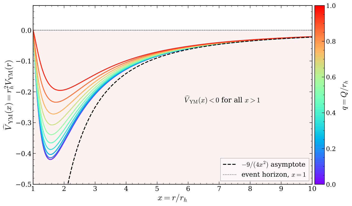
Equation (6.3) vanishes at the horizon, where . Far away it approaches
| (6.4) |
which is negative. The potential is therefore not positive definite, and no positivity argument can establish stability, exactly as found in the original five-dimensional analysis [45]. A direct eigenvalue calculation is unavoidable, and as Sec. 6.4 shows, the coefficient in Eq. (6.4) does considerably more than block a positivity proof.
6.2 Dimensionless form and boundary conditions
For the numerical work we set
| (6.5) |
so that the nonextremal branch is and the extremal configuration is approached as , equivalently . The metric function and effective potential become
| (6.6) |
and the master equation reads
| (6.7) |
Figure 4 plots across the nonextremal range. The potential is negative everywhere outside the horizon for every charge examined. Increasing makes the well shallower and pushes its minimum outward, but never lifts the potential above zero, and the asymptotic tail (6.4) is independent of altogether.
With the convention the quasinormal boundary conditions are at the horizon and at infinity. The negativity of singles out a simple subclass, the purely imaginary modes. Writing
| (6.8) |
Eq. (6.7) turns into the bound-state problem
| (6.9) |
whose boundary conditions are exponential decay at both ends, near the horizon and at large radius. Negative eigenvalues of the Schrödinger operator in Eq. (6.9) are therefore in one-to-one correspondence with unstable modes, and a positive imaginary part of means exponential growth in time.
6.3 Numerical spectrum
We solve Eq. (6.9) by two independent methods and use their agreement as the error estimate.
The first is direct diagonalization. We integrate the background from on a uniform tortoise grid, discretize the one-dimensional Schrödinger operator to second order in the grid spacing, impose Dirichlet conditions on the numerically decayed master function at both ends, and diagonalize the resulting symmetric tridiagonal matrix. Negative eigenvalues convert to growth rates through .
The second is a Riccati shooting scheme, which avoids the exponential range problem that afflicts naive two-point shooting over a long tortoise interval. Setting , Eq. (6.9) becomes
| (6.10) |
The horizon is a fixed point of Eq. (6.10) at , so the inner boundary condition must be started from its first-order expansion. With and one finds
| (6.11) |
while at large the decaying solution gives . Integrating inward and outward and matching at fixes . Because the fundamental mode has no node, stays finite throughout and the scheme is well conditioned.
Table 3 reports the fundamental growth rate from both methods across the nonextremal range. The two schemes agree to or better at every charge, and the residual is dominated by the second-order truncation of the finite-difference operator, as confirmed by Richardson extrapolation in the grid spacing. The lowest eigenvalue is also insensitive to the computational domain: shifting the outer boundary from to leaves unchanged in the sixth decimal place.
The spectrum is unstable everywhere on the nonextremal branch. At the thermodynamically distinguished radius , that is ,
| (6.12) |
and the growth rate falls monotonically with charge, from in the limit, where the potential reduces to its Schwarzschild–Tangherlini form, to at . The decrease is gentle: over the whole nonextremal range the rate drops by less than a quarter. This weakening toward extremality should not be read as stability at extremality. It says only that the dimensionless growth rate diminishes as , and the exact extremal point lies outside the reach of the present scheme because the surface gravity vanishes there and the tortoise coordinate degenerates.
The comparison with the thermodynamics is the point of Fig. 5(a). The Davies scale is where diverges and the local stability of the horizon reverses. The instability rate notices nothing. It varies smoothly through that charge, with no kink, no divergence and no change of slope beyond the smooth trend already present on either side. Within this perturbation sector the Davies-type transition carries no dynamical signature.
| (finite difference) | (shooting) | difference | |
|---|---|---|---|
| 0.41475258 | 0.41475247 | ||
| 0.41460925 | 0.41460914 | ||
| 0.41417731 | 0.41417720 | ||
| 0.41242008 | 0.41241997 | ||
| 0.40938223 | 0.40938213 | ||
| 0.40488359 | 0.40488350 | ||
| 0.39863427 | 0.39863419 | ||
| 0.39232194 | 0.39232187 | ||
| 0.38492835 | 0.38492830 | ||
| 0.37883389 | 0.37883384 | ||
| 0.36349146 | 0.36349142 | ||
| 0.34252255 | 0.34252252 | ||
| 0.32936329 | 0.32936327 | ||
| 0.31751959 | 0.31751957 |
6.4 An accumulating tower of unstable modes
The fundamental mode is not the whole spectrum. The asymptotic form (6.4) is an attractive inverse-square tail, with , and the bound-state problem for such a tail is governed by the sign of . Writing the tail as with gives and
| (6.13) |
which is real. This is the classic supercritical case [19, 24]: the effective radial exponent becomes imaginary, the operator is unbounded below in the absence of a short-distance cutoff, and the discrete spectrum accumulates geometrically at zero energy. The horizon supplies the cutoff here, so the fundamental mode is finite and well defined, but the tower above it is not truncated. The eigenvalues satisfy at large , hence
| (6.14) |
The ratio is fixed by the coefficient of the tail alone. Since that coefficient is for every , the accumulation rate is independent of the Yang–Mills charge even though the individual are not.
Table 4 tests this. At three representative charges the first four growth rates were computed on domains extended to , which is required because each successive overtone is spatially an order of magnitude broader than the last. The successive ratios approach Eq. (6.14) from above, reaching , and by at , and respectively, in agreement with the predicted to the accuracy the domain permits. Pushing the outer boundary to resolves a fifth mode at and gives the next ratio as . Figure 5(b) displays the tower and the convergence of the ratios.
Two remarks are in order. First, only is a domain-independent number; the higher members are physical but require progressively larger domains to resolve, and any truncation of the exterior region artificially terminates the tower. Second, the accumulation does not make the instability worse in any practical sense. The growth is dominated by , and the overtones are slower by an order of magnitude at each step. Their significance is structural: the magnetic sector of this geometry has no gap above the fundamental unstable mode, which is a property of the long-range tail rather than of the horizon.
| 0.4141778 | 0.0748221 | 0.0086664 | 0.0009412 | 0.1807 | 0.1158 | 0.1086 | |
| 0.3923223 | 0.0864727 | 0.0106115 | 0.0011546 | 0.2204 | 0.1227 | 0.1088 | |
| 0.3425227 | 0.1122088 | 0.0191906 | 0.0021407 | 0.3276 | 0.1710 | 0.1116 |

6.5 Scope of the calculation
Two limitations should be stated plainly. The calculation perturbs the magnetic Yang–Mills configuration and eliminates the accompanying metric perturbations through the linearized field equations, so it is a genuine stability test of the gauge sector rather than a probe-field spectrum. It is not, however, the full quasinormal spectrum of the higher-dimensional Wu–Yang system. A complete treatment would decompose tensor, vector, scalar and internal-gauge perturbations of the configuration in the Kodama–Ishibashi formalism [34, 35, 32], which is a considerably heavier problem and is left for future work. Other sectors could in principle carry different stability properties, though the four-dimensional precedent [51, 11, 12] does not encourage optimism.
The second limitation concerns the entropy correction. Section 4 treats as a modification of the entropy at fixed metric, so the perturbation problem solved here is the classical one. A self-consistent treatment would correct the field equations and hence the potential (6.3) itself [16], and only then could the effect of on be quantified. Since the correction is exponentially confined to the near-horizon region while is set by the well between the horizon and , we expect the effect to be small but do not claim it.
7 Discussion and conclusions
We have assembled a description of the five-dimensional Einstein–Yang–Mills black hole of Mazharimousavi and Halilsoy [42] that carries exact thermodynamics, a non-perturbative entropy correction, a global topological classification, and a direct test of the stability of the non-Abelian sector.
At the classical level the analysis closes in elementary functions. The horizon condition gives the mass–radius relation (2.7), the temperature collapses to the compact form (3.1), the extremal radius is and the extremal mass follows in closed form. The area law supplies the entropy, the first law is satisfied identically, and the conjugate Yang–Mills potential (3.7) completes the set. Two corrections to the existing literature emerged along the way. The Gibbs-like potential is Eq. (3.11), in which the logarithmic term changes sign relative to the Helmholtz free energy, and the corrected heat capacity carries the prefactor of Eq. (4.5). We also recorded the curvature invariants, Eqs. (2.8) and (2.9), which show that the logarithm in the metric function strengthens rather than regulates the central singularity.
The classical heat capacity diverges at , a Davies-type point [22] whose interpretation has been reconsidered recently [6]. Adding the exponential correction (4.1) moves that point inward, and the weak-correction expansion (4.9) gives the displacement in closed form. At the shift reaches almost by . This behavior parallels what has been found in logarithmic nonlinear electrodynamics backgrounds [18], dilaton gravity [13], AdS–Rindler geometries [15] and Lifshitz black holes [17]: the exponential term reorganizes the small-horizon sector and leaves the large-horizon thermodynamics intact.
The topological description makes that statement precise. The defect equation (5.3) turns out to be the corrected temperature itself, which ties the winding-number classification directly to the local analysis. At fixed we find a defect pair with and and total charge , unchanged for every correction strength examined, in line with the general expectation that the topological number depends on the asymptotic thermodynamics at small and large horizon radius rather than on the details in between [61, 62]. What the correction does is move the stable member of the pair while leaving the unstable member fixed to six decimal places, because the exponential is suppressed by eleven orders of magnitude at the outer defect. Non-perturbative quantum corrections deform the near-horizon thermodynamics and preserve the global classification, which matches the pattern reported for other entropy-corrected systems [18, 13, 15, 17, 25, 26].
The dynamical results are the part that does not follow from the thermodynamics. Perturbing the magnetic Yang–Mills configuration itself, in the framework of Okuyama and Maeda [45], we found a purely imaginary unstable mode across the whole nonextremal range, with falling monotonically from at vanishing charge to at . Two independent numerical schemes agree to better than . The mode passes through the Davies scale without any feature, so within this sector a divergence of the heat capacity is not accompanied by a divergent or even an anomalous dynamical timescale. That is worth contrasting with holographic settings where quasinormal frequencies do track thermodynamic transitions in the dual theory [38, 31]: the correspondence between thermodynamic singularities and dynamical response is evidently more delicate for intrinsic gauge-field perturbations than for probe fields.
The tower of Sec. 6.4 was not anticipated. Because the effective potential decays as and the coefficient exceeds the critical value for an inverse-square tail, the sector supports infinitely many unstable modes accumulating at with the ratio . Our numerics reproduce that constant at three different charges, as they must, since it depends on the tail coefficient and nothing else. The magnetic sector therefore has no spectral gap above its fundamental instability, and the absence of a gap is a property of the asymptotic region rather than of the horizon.
These results place the geometry in context. Hendi and Nemati studied five-dimensional Yang–Mills massive gravity and reported van der Waals behavior together with scalar WKB frequencies [31], but for planar horizons in the extended phase space; our setting is spherical, with a logarithmic metric function, exponential entropy corrections and a topological classification. Guo and Miao showed that the logarithm removes the divergence of the Hawking temperature while preserving a charge-dependent scalar spectrum [28, 27]; the magnetic sector studied here answers the different question of whether the solution holds together, and the answer is that it does not. Pu and Yang found that regular EYM frequencies approach the Schwarzschild values at large charge [49], whereas the purely imaginary mode found here persists across the entire charge range. Analyzing gauge-field perturbations directly, rather than relying on scalar probes, changes the conclusion.
A number of extensions follow naturally. Restoring a cosmological constant would open the EYM–AdS phase structure, with Hawking–Page and van der Waals behavior and a holographic reading of the entropy correction [31, 3]. Moving to Einstein–Yang–Mills–Gauss–Bonnet theory [41] would show how higher-curvature terms interact with the non-Abelian charge and the exponential correction. A side-by-side comparison of logarithmic and exponential corrections in the same background would clarify which scheme is appropriate in which regime [20, 47]. The complete perturbation problem remains open, as does the behavior of at exact extremality, which needs numerical techniques adapted to vanishing surface gravity. Finally, a self-consistent treatment in which the exponential correction back-reacts on the metric [16] would let the entropy correction and the instability rate be computed within a single scheme, which is the natural next step for this system.
Acknowledgments
İ. S. thanks EMU, TÜBİTAK, ANKOS and SCOAP3 for their support. He also acknowledges COST Actions CA22113, CA21106, CA23130, CA21136 and CA23115 for their contributions to networking. The authors thank the anonymous referees for comments that improved the manuscript.
Data Availability Statement
The data supporting the findings of this study are contained within the article. The numerical scripts used to generate the tables and figures, covering the symbolic verification of the thermodynamic relations, the defect and transition-radius roots, and the finite-difference and Riccati eigenvalue solvers, are available from the corresponding author on reasonable request.
References
- [1] (2026) Quantum-modified Regge-Wheeler Formalism for Black Holes with Phantom Global Monopoles: Potential Profiles and Quasinormal Modes. Int. J. Geom. Meth. Mod. Phys. 23, pp. 2550257. External Links: Document, Link Cited by: §1.
- [2] (2026) Thermodynamics of Charged Bardeen-AdS Black Hole with Perfect Fluid Dark Matter and Cloud of Strings. Nucl. Phys. B 1029, pp. 117531. External Links: Document, Link Cited by: §1.
- [3] (2024) Topology of Born-Infeld-AdS Black Hole Phase Transitions: Bulk and CFT Sides. Annals Phys. 465, pp. 169679. External Links: Document, Link Cited by: §1, §5, §7.
- [4] (2023) Topological Classification and Black Hole Thermodynamics. Phys. Dark Univ. 42, pp. 101361. External Links: Document, Link Cited by: §1, §5.
- [5] (1973) The Four Laws of Black Hole Mechanics. Commun. Math. Phys. 31, pp. 161. External Links: Document, Link Cited by: §1.
- [6] (2024) Physical Reinterpretation of Heat Capacity Discontinuities for Static Black Holes. Phys. Rev. D 110, pp. 124035. External Links: Document, Link Cited by: §3, §7.
- [7] (1988) Particle-like Solutions of the Einstein-Yang-Mills Equations. Phys. Rev. Lett. 61, pp. 141. External Links: Document, Link Cited by: §1, §1.
- [8] (1973) Black Holes and Entropy. Phys. Rev. D 7, pp. 2333. External Links: Document, Link Cited by: §1, §3.
- [9] (2009) Quasinormal Modes of Black Holes and Black Branes. Class. Quant. Grav. 26, pp. 163001. External Links: Document, Link Cited by: §1.
- [10] (1990) Colored Black Holes. Phys. Rev. Lett. 64, pp. 2844. External Links: Document, Link Cited by: §1, §1.
- [11] (1991) Stability of Einstein-Yang-Mills Black Holes. Phys. Lett. B 259, pp. 53. External Links: Document, Link Cited by: §1, §1, §6.5, §6.
- [12] (1996) Instability Proof for Einstein-Yang-Mills Solitons and Black Holes with Arbitrary Gauge Groups. J. Math. Phys. 37, pp. 1414. External Links: Document, Link Cited by: §1, §1, §6.5, §6.
- [13] (2026) Exact Black-Hole Solutions in Dilaton Gravity: Thermodynamics, Stability, Topology, and Dynamical Probes. Nucl. Phys. B 1029, pp. 117588. External Links: Document, Link Cited by: §1, §1, §7, §7.
- [14] (2025) Quantum-Corrected Thermodynamics of AdS-Rindler Black Holes. East Eur. J. Phys. 4, pp. 75. External Links: Document, Link Cited by: §1.
- [15] (2026) Entropy-driven Reorganization of Thermodynamic Topology in AdS-Rindler Black Holes. Phys. Lett. B 879, pp. 140642. External Links: Document, Link Cited by: §1, §1, §7, §7.
- [16] (2026) Exponential Corrected Metric of the 3D BTZ Black Hole. Can. J. Phys. 104, pp. 1. External Links: Document, Link Cited by: §1, §6.5, §7.
- [17] (2026) Planck-Scale Deformation of Thermodynamic Topology and Stability in Lifshitz Black Holes. Class. Quant. Grav. 43, pp. 145019. External Links: Document, Link Cited by: §1, §1, §7, §7.
- [18] (2026) Stability and Thermodynamic Topology of Logarithmic Nonlinear Electrodynamics Black Holes with Exponential Entropy Corrections. Phys. Lett. B 877, pp. 140490. External Links: Document, Link Cited by: §1, §1, §7, §7.
- [19] (1950) Singular Potentials. Phys. Rev. 80, pp. 797. External Links: Document, Link Cited by: §6.4.
- [20] (2020) Exponential Corrections to Black Hole Entropy. Phys. Rev. Lett. 125, pp. 041302. External Links: Document, Link Cited by: §1, §4, §7.
- [21] (1995) Quantum Corrections to Black Hole Entropy in String Theory. Phys. Lett. B 347, pp. 222. External Links: Document, Link Cited by: §1.
- [22] (1989) Thermodynamic Phase Transitions of Kerr-Newman Black Holes in de Sitter Space. Class. Quant. Grav. 6, pp. 1909. External Links: Document, Link Cited by: §3, §7.
- [23] (2000) Topological Tensor Current of -Branes in the -Mapping Theory. J. Math. Phys. 41, pp. 4379. External Links: Document, Link Cited by: §1, §5.
- [24] (1971) Singular Potentials. Rev. Mod. Phys. 43, pp. 36. External Links: Document, Link Cited by: §6.4.
- [25] (2025) Thermodynamic Topology and Phase Space Analysis of AdS Black Holes through Non-extensive Entropy Perspectives. Eur. Phys. J. C 85, pp. 305. External Links: Document, Link Cited by: §1, §7.
- [26] (2025) Thermodynamic Topology, Photon Spheres, and Evidence for the Weak Gravity Conjecture in Charged Black Holes with Perfect Fluid within Rastall Theory. Phys. Lett. B 869, pp. 139862. External Links: Document, Link Cited by: §1, §7.
- [27] (2020) Null Geodesics, Quasinormal Modes, and the Correspondence with Shadows in High-dimensional Einstein-Yang-Mills Spacetimes. Phys. Rev. D 102, pp. 084057. External Links: Document, Link Cited by: §1, §6, §7.
- [28] (2020) Scalar Quasinormal Modes of Black Holes in Einstein-Yang-Mills Gravity. Phys. Rev. D 102, pp. 064049. External Links: Document, Link Cited by: §1, §6, §7.
- [29] (1975) Particle Creation by Black Holes. Commun. Math. Phys. 43, pp. 199. External Links: Document, Link Cited by: §1.
- [30] (1976) Black Holes and Thermodynamics. Phys. Rev. D 13, pp. 191. External Links: Document, Link Cited by: §1.
- [31] (2019) Thermodynamics, Shadow and Quasinormal Modes of Black Holes in Five-dimensional Yang-Mills Massive Gravity. Note: arXiv:1912.06824 [gr-qc] External Links: 1912.06824, Link Cited by: §7, §7, §7.
- [32] (2011) Perturbations and Stability of Static Black Holes in Higher Dimensions. Prog. Theor. Phys. Suppl. 189, pp. 165. External Links: Document, Link Cited by: §1, §6.5.
- [33] (1994) Some Properties of Noether Charge and a Proposal for Dynamical Black Hole Entropy. Phys. Rev. D 50, pp. 846. External Links: Document, Link Cited by: §1.
- [34] (2003) A Master Equation for Gravitational Perturbations of Maximally Symmetric Black Holes in Higher Dimensions. Prog. Theor. Phys. 110, pp. 701. External Links: Document, Link Cited by: §1, §6.5.
- [35] (2004) Master Equations for Perturbations of Generalized Static Black Holes with Charge in Higher Dimensions. Prog. Theor. Phys. 111, pp. 29. External Links: Document, Link Cited by: §6.5.
- [36] (1999) Quasi-normal Modes of Stars and Black Holes. Living Rev. Rel. 2, pp. 2. External Links: Document, Link Cited by: §1.
- [37] (2019) Higher Order WKB Formula for Quasinormal Modes and Grey-body Factors: Recipes for Quick and Accurate Calculations. Class. Quant. Grav. 36, pp. 155002. External Links: Document, Link Cited by: §6.
- [38] (2011) Quasinormal Modes of Black Holes: From Astrophysics to String Theory. Rev. Mod. Phys. 83, pp. 793. External Links: Document, Link Cited by: §1, §7.
- [39] (2003) Quasinormal Behavior of the -dimensional Schwarzschild Black Hole and the Higher Order WKB Approach. Phys. Rev. D 68, pp. 024018. External Links: Document, Link Cited by: §1, §6.
- [40] (2017) Quasinormal Modes of Black Holes: The Improved WKB Approach. Phys. Rev. D 96, pp. 024011. External Links: Document, Link Cited by: §6.
- [41] (2007) 5D Black Hole Solution in Einstein-Yang-Mills-Gauss-Bonnet Theory. Phys. Rev. D 76, pp. 087501. External Links: Document, Link Cited by: §1, §2, §2, §7.
- [42] (2008) Einstein-Yang-Mills Black Hole Solution in Higher Dimensions by the Wu-Yang Ansatz. Phys. Lett. B 659, pp. 471. External Links: Document, Link Cited by: §1, §2, §2, §2, §2, §7.
- [43] (2009) Effect of the Born-Infeld Parameter in Higher Dimensional Hawking Radiation. Phys. Lett. B 672, pp. 177. External Links: Document, Link Cited by: §1.
- [44] (1999) Quasinormal Modes: The Characteristic Sound of Black Holes and Neutron Stars. Class. Quant. Grav. 16, pp. R159. External Links: Document, Link Cited by: §1.
- [45] (2003) Five-dimensional Black Hole and Particle Solution with a Non-Abelian Gauge Field. Phys. Rev. D 67, pp. 104012. External Links: Document, Link Cited by: §1, §6.1, §6.1, §7.
- [46] (2021) Quantum Corrections to the Thermodynamics of Black Branes. JHEP 10, pp. 050. External Links: Document, Link Cited by: §1, §4.
- [47] (2024) Non-perturbative Correction on the Black Hole Geometry. Phys. Dark Univ. 44, pp. 101444. External Links: Document, Link Cited by: §1, §4, §7.
- [48] (2025) Thermal Fluctuation Effects on Shear Viscosity to Entropy Ratio in Five-dimensional Kerr-Newman Black Holes. Eur. Phys. J. C 85, pp. 206. External Links: Document, Link Cited by: §1.
- [49] (2023) Quasinormal Ringing of Regular Einstein-Yang-Mills Black Hole. EPL 144, pp. 44001. External Links: Document, Link Cited by: §7.
- [50] (1993) Existence of Black Hole Solutions for the Einstein-Yang/Mills Equations. Commun. Math. Phys. 154, pp. 377. External Links: Document, Link Cited by: §1, §1.
- [51] (1990) Instability of a Colored Black Hole Solution. Phys. Lett. B 243, pp. 33. External Links: Document, Link Cited by: §1, §1, §6.5, §6.
- [52] (2026) Multi-spin Particle Tunneling and Black Hole Thermodynamics: GUP-corrected Zitterbewegung and Exponentially Modified Entropy. Phys. Lett. B 875, pp. 140282. External Links: Document, Link Cited by: §1.
- [53] (2026) Unified Analysis of Fermionic Tunneling, Barrow-Exponential Entropy Corrections, and Plasma Lensing in Carrollian Reissner-Nordström Spacetime. Annalen Phys. 538, pp. e00588. External Links: Document, Link Cited by: §1.
- [54] (2025) Exploring Lorentz-violating Effects of the Kalb-Ramond Field on Charged Black Hole Thermodynamics and Photon Dynamics. Phys. Rev. D 111, pp. 064049. External Links: Document, Link Cited by: §1.
- [55] (2025) Quantum Tunneling and Aschenbach Effect in Nonlinear Einstein-Power-Yang-Mills AdS Black Holes. Chin. Phys. C 49, pp. 105101. External Links: Document, Link Cited by: §1.
- [56] (1963) Schwarzschild Field in Dimensions and the Dimensionality of Space Problem. Nuovo Cim. 27, pp. 636. External Links: Document, Link Cited by: §1, §2.
- [57] (2025) Black Hole Thermodynamics and Stability in Einstein-Yang-Mills Gravity with Quantum Fluctuation-Induced Corrections. Prog. Theor. Exp. Phys. 2025, pp. 083E02. External Links: Document, Link Cited by: §1, §2, §2.
- [58] (2023) Some Observable Physical Properties of the Higher Dimensional dS/AdS Black Holes in Einstein-Bumblebee Gravity Theory. Eur. Phys. J. C 83, pp. 668. External Links: Document, Link Cited by: §1.
- [59] (1993) Black Hole Entropy is Noether Charge. Phys. Rev. D 48, pp. R3427. External Links: Document, Link Cited by: §1.
- [60] (2001) The Thermodynamics of Black Holes. Living Rev. Rel. 4, pp. 6. External Links: Document, Link Cited by: §1, §2, §3.
- [61] (2022) Black Hole Solutions as Topological Thermodynamic Defects. Phys. Rev. Lett. 129, pp. 191101. External Links: Document, Link Cited by: §1, §5, §7.
- [62] (2022) Topology of Black Hole Thermodynamics. Phys. Rev. D 105, pp. 104003. External Links: Document, Link Cited by: §1, §5, §7.
- [63] (1975) Solutions for Gravity Coupled to Massless Gauge Fields. Phys. Rev. D 12, pp. 2212. External Links: Document, Link Cited by: §1, §1, §2, §2.