Partition the Support, Reconstruct the
Residual: Training-Free Sparse Attention for Video Generation and World Models

Pardis Taghavi Reza Langari Gaurav Pandey Affiliation: Texas A&M University Email: {ptgh,rlangari,gpandey}@tamu.edu

Abstract

Training-free block-sparse attention can accelerate video transformers, but row-wise attention concentration does not by itself specify an executable sparse operator. Queries sharing a block route may have poorly overlapping supports, while retained attention mass alone does not determine the post-softmax error from skipped interactions. We show that partition geometry affects both pooled support and the predictability of the remaining residual from the sparse output. We introduce SparsePR, which combines Response-Coupled Partitioning with Probe-Fitted Residual Reconstruction. Sampled-query key responses form paired K/V groups, whose centroids induce query-response coordinates for shared routing. A small set of exact query rows then calibrates a call-specific affine correction from the sparse output within the output subspace observed in the probe residuals. Across four heterogeneous video generation and world models, SparsePR consistently reduces attention-reconstruction error. Ablations show that probe fitting accounts for most of this reduction, while response-coupled partitioning lowers hard-drop error and improves reconstruction under a finite probe budget. SparsePR preserves generation quality at 22.0–26.0% realized executed-pair density while achieving 1.48×–2.61× end-to-end speedups. Project page

1 Introduction

Video generation models (13; 30; 37) and video world models for physical world prediction (21; 22) process long spatiotemporal token sequences, making quadratic self-attention a major inference bottleneck at high resolution and long duration. Pretrained video DiTs often exhibit structured, head-dependent attention concentration (3; 26; 19), motivating training-free sparse attention for accelerating pretrained models. Prior methods exploit spatiotemporal structure, estimate important blocks online, reorder tokens into executable layouts, or approximate skipped interactions (41; 32; 33; 39; 35; 36; 44; 15). Yet row-wise attention concentration does not determine the support needed when queries share executable block routes, and retained attention mass does not determine the post-softmax error from skipped interactions. These issues are particularly relevant in video world models, where conditioning and prediction regimes can induce different attention structures. An executable sparse operator must therefore account for both shared-route support and the output error from skipped interactions, rather than treating sparsity as a row-wise property alone.

We analyze this challenge by separating the choices that define an executable block-sparse attention computation. The query partition determines which rows share a routing decision, the paired K/V partition determines which tokens are selected together at block granularity, the routing policy selects the cells evaluated exactly, and the skipped-interaction rule specifies how the remaining pairs affect the output. Our analysis reveals three dependencies across the evaluated models. First, per-query concentration does not determine shared-route support. Under the semantic partition, Wan2.2 requires a median support of $6.2\%$ per query to retain $90\%$ of the attention mass, but $22.9\%$ when eight grouped queries share one route. In contrast, Cosmos-Predict2.5 exhibits denser support at the individual-row level. High shared-route density can therefore arise either from weak support agreement within a query group or intrinsic row density. Second, retained attention mass does not determine post-softmax accuracy. Under renormalized hard drop, the residual depends on both the omitted mass and the difference between the outputs induced by the omitted and retained supports. Routes with comparable retained mass can therefore produce different output errors. Cosmos3-Nano exhibits this sensitivity in our sparse runs, motivating direct measurement of post-softmax error rather than inferring output behavior from retained mass or exact-pair density. Third, under matched sparse execution, partition choice changes how much of the remaining residual can be represented by an affine function of the sparse output. Partition geometry therefore affects both the support required for shared execution and the structure of the residual left for reconstruction.

Refer to caption — Figure 1: Qualitative Results. Cosmos2.5-14B mdoel.

Motivated by these observations, we introduce SparsePR, a training-free sparse-attention framework that combines Response-Coupled Partitioning with Probe-Fitted Residual Reconstruction. Response-Coupled Partitioning constructs paired K/V and query partitions through a single asymmetric pass over response coordinates derived from the current attention call. Sampled queries define key-response coordinates for paired K/V grouping, and the resulting key-group centroids define query-response coordinates for shared routing. Probe-Fitted Residual Reconstruction evaluates a small set of query rows exactly and fits a call-specific affine map from the sparse output to the corresponding post-softmax residual. The fitted map estimates residual on unprobed rows. All partitioning and residual calibration are performed online without offline training. Unlike prior methods that couple query and key groups for routing or approximate skipped interactions from block-level approximations (19; 44; 15; 14), SparsePR combines current-call response partitioning with exact row calibrated post-softmax residual reconstruction.

We make three contributions. First, we characterize dependencies that shape executable block-sparse attention across four video models. Per-query concentration does not determine shared-route support, high retained attention mass does not guarantee low post-softmax error, and partition choice changes how much of the residual can be represented by an affine function of the sparse output. Second, we introduce SparsePR, which combines Response-Coupled Partitioning with Probe-Fitted Residual Reconstruction in an online, training-free sparse-attention framework. Third, we evaluate SparsePR across four models using exact-pair accounting that includes probe rows and end-to-end timing that includes online overheads. SparsePR closely matches dense benchmark quality while achieving $1.48\times$ to $2.61\times$ end-to-end speedups.

Figure 2: Overview of SparsePR. Response-Coupled Partitioning builds executable K/V and query groups, and Probe-Fitted Residual Reconstruction uses exact probe rows to correct the sparse output.

2 Related Work

Sparse Attention for Video Generative Models and Video World Models.

Training-free sparse attention for video DiTs reduces inference cost through structured sparse patterns, online block selection, or current-call support estimation. Sliding Tile Attention, SVG, Sparse-vDiT, Radial Attention, LVSA, and VORTA exploit spatial, temporal, layer, or head structures (41; 32; 3; 17; 8; 26). AdaSpa, SpargeAttention, and XAttention estimate important blocks from the current attention call (33; 39; 35), while HASTE and ScalingAttention reduce repeated support-estimation cost through temporal mask reuse or offline topology priors (42; 43). VSA and VEDA learn sparse execution through end-to-end training or distillation, while VMoBA supports both sparse training and training-free inference (40; 9; 31). Exact dense kernels such as FlashAttention are complementary because they preserve dense attention support (6). In autoregressive video models, sparse attention has also been used for causal K/V cache compression and approximate retrieval (24). Our setting considers full-sequence attention and studies how partitioning and skipped-interaction treatment determine executable density and post-softmax error.

Token Partitioning for Executable Block Sparsity.

Earlier methods for general Transformers organized tokens through LSH, online $k$ -means, query clustering, asymmetric clustering, and learned permutations (12; 23; 29; 7; 28). For video DiTs, SVG2 clusters query and key activations and permutes the resulting groups into contiguous layouts (36). DraftAttention and DFSAttn use coarse attention guidance or hierarchical ordering to expose executable block structure (25; 10). AdaCluster uses different similarity criteria for queries and keys, while SVOO iteratively alternates query-aware key clustering and key-aware query clustering (27; 19). Response-Coupled Partitioning instead uses a single asymmetric coupling pass. Key responses under sampled queries define paired K/V groups, nd the resulting key-group centroids induce query coordinates without alternating partition refinement.

Attention Approximation and Residual Reconstruction.

Attention approximations use random features, landmarks, or sparse and low-rank approximations (5; 34; 2). Sparse attention methods for visual generation instead approximate or recover contributions from skipped interactions. Re-ttention reuses softmax statistics across denoising steps, Rectified SpaAttn applies pooled corrections, PSA retains multiresolution K/V representations, and SVG-EAR compensates skipped semantic blocks using K/V centroids and error-aware routing (4; 18; 16; 44). PISA and Sol-Attn approximate omitted contributions using blockwise Taylor expansions and routing proxy scores, respectively (15; 14). SparsePR instead uses a small set of exact exact query rows to fit a map from the sparse output to the residual, without temporal reuse or offline training.

3 Sparse Attention Formulation and Observations

Block-sparse attention makes sparsity executable by grouping tokens and evaluating selected query–key group pairs. The resulting operator is determined by partition construction, route selection, and the treatment of skipped interactions. These choices introduce distinct sources of approximation error. We formalize this operator and identify three structural dependencies that motivate SparsePR.

Dense and block-sparse attention.

For one attention head, let $Q\in\mathbb{R}^{N_{q}\times d}$ , $K\in\mathbb{R}^{N_{k}\times d}$ , and $V\in\mathbb{R}^{N_{k}\times d_{v}}$ . Dense attention computes

A=\operatorname{softmax}\!\left(\frac{QK^{\top}}{\sqrt{d}}\right),\qquad O^{\mathrm{dense}}=AV.

(1)

A block-sparse operator partitions queries into $\mathcal{G}^{Q}=\{G_{a}^{Q}\}_{a=1}^{C_{q}}$ and K/V tokens into $\mathcal{G}^{KV}=\{G_{b}^{KV}\}_{b=1}^{C_{k}}$ . Each pair $G_{a}^{Q}\times G_{b}^{KV}$ defines a cell. Let $z_{ab}\in\{0,1\}$ indicate whether the cell is evaluated exactly. To account for unequal group sizes, the routing density over query–key pairs is

\rho_{\mathrm{route}}=\frac{1}{N_{q}N_{k}}\sum_{a=1}^{C_{q}}\sum_{b=1}^{C_{k}}z_{ab}\lvert G_{a}^{Q}\rvert\lvert G_{b}^{KV}\rvert.

(2)

Under renormalized hard drop, every query $i\in G_{a}^{Q}$ uses the same retained K/V groups. Let $K_{a}$ and $V_{a}$ collect the key and value rows from groups $G_{b}^{KV}$ with $z_{ab}=1$ . The sparse output is

O_{i}^{\mathrm{sp}}=\operatorname{softmax}\!\left(\frac{q_{i}K_{a}^{\top}}{\sqrt{d}}\right)V_{a}.

(3)

Collecting these rows gives $O^{\mathrm{sp}}$ , with post-softmax residual

R=O^{\mathrm{dense}}-O^{\mathrm{sp}}.

Here, $\rho_{\mathrm{route}}$ counts pairs evaluated by sparse routing. Total executed-pair density additionally includes exact probe rows, as defined in Section 4.3.

3.1 Structural Observations on Sparse Attention

We use semantic clustering as a reference partition, applying k-means separately to the current query and key activations, with each value token inheriting the assignment of its paired key (36). We use this partition to examine support expansion under shared routing, post-softmax error under renormalized hard drop, and the affine representability of the residual from the sparse output.

O1: Per-Query Sparsity Does Not Determine Shared-Route Support.

For a target retained mass $\alpha\in(0,1]$ , let $D_{i}(\alpha)$ denote the smallest set of highest-weight key indices whose cumulative dense attention mass for query $i$ is at least $\alpha$ . For $m$ queries $i_{1},\ldots,i_{m}\in G_{a}^{Q}$ , define

\tau_{i}(\alpha)=\frac{\lvert D_{i}(\alpha)\rvert}{N_{k}},\qquad\gamma_{a}^{(m)}(\alpha)=\frac{\left\lvert\bigcup_{r=1}^{m}D_{i_{r}}(\alpha)\right\rvert}{N_{k}}.

Here, $\tau_{i}(\alpha)$ measures row-wise support density, while $\gamma_{a}^{(m)}(\alpha)$ measures pooled support density. Because the union is formed over individual key indices, this diagnostic isolates query-side support disagreement before further expansion from selecting K/V groups. Under the semantic partition, Fig. 3(a) compares per-query and pooled support at $\alpha=0.9$ . Vertical displacement above the diagonal measures support expansion from limited overlap among key supports. Wan2.2 is the clearest example: its median support increases from $6.2\%$ per query to $22.9\%$ after pooling. Cosmos-Predict2.5 is broad at the row level, with median support increasing from $56.5\%$ to $77.7\%$ after pooling. HunyuanVideo remains sparse at both levels, while Cosmos3-Nano occupies an intermediate regime. Pooled support therefore depends on both row-wise concentration and support overlap within query groups, showing why per-query sparsity alone does not characterize shared routing.

Figure 3: Structural observations under the semantic reference partition. (a) Per-query versus eight-query pooled support at

90\%

attention mass. Vertical displacement above the diagonal indicates support expansion under pooling. (b) p99 normalized attention-output error versus realized retained attention mass. Comparable retained mass can produce different post-softmax errors across models.

O2: Retained Attention Mass Alone Does Not Determine Output Error.

For $i\in G_{a}^{Q}$ , let $U_{a}$ denote the omitted key indices and $p_{U,i}=\sum_{j\in U_{a}}A_{ij}$ be omitted mass. Let $O_{U,i}$ denote the output obtained by renormalizing the dense attention weights over $\mathcal{U}_{a}$ . The residual then satisfies:

R_{i}=O_{i}^{\mathrm{dense}}-O_{i}^{\mathrm{sp}}=p_{U,i}\left(O_{U,i}-O_{i}^{\mathrm{sp}}\right).

(4)

Thus, high retained mass makes $p_{U,i}$ small, but does not constrain $\lVert O_{U,i}-O_{i}^{\mathrm{sp}}\rVert_{2}$ . Queries with similar retained mass can therefore have different residual norms. Figure 3(b) shows that error generally decreases as retained mass increases, but model-dependent variation remains at comparable mass levels. High retained attention mass alone is insufficient to characterize post-softmax error.

O3: Partition Geometry Changes Residual Representability

Residual magnitude alone does not indicate how well the hard-drop residual can be represented by an affine function of the sparse output. Let $g$ index a choice of query and K/V partitions, with sparse output $O_{g}^{\mathrm{sp}}$ and corresponding post-softmax residual $R_{g}$ . Define the affine feature matrix

X_{g}=[\mathbf{1},\,O_{g}^{\mathrm{sp}}],

and let $P_{X_{g}}$ denote the orthogonal projector onto $\operatorname{col}(X_{g})$ . The residual decomposes as

R_{g}=\underbrace{P_{X_{g}}R_{g}}_{\text{affine-explainable component}}+\underbrace{(I-P_{X_{g}})R_{g}}_{\text{affine-orthogonal residual}}.

(5)

For $X_{g}$ , the projected term is the best least-squares approximation of $R_{g}$ by an affine function of $O_{g}^{\mathrm{sp}}$ , while the orthogonal term lies outside this feature space. Computing this decomposition requires the full dense residual, and it serves as an oracle diagnostic rather than part of sparse execution.

We compare the semantic and response-coupled partitions from Section 4.1 under matched group counts, routing, renormalized hard drop, and realized pair density. We report the fraction of residual energy captured by the affine feature space, $\lVert P_{X_{g}}R_{g}\rVert_{F}^{2}/\lVert R_{g}\rVert_{F}^{2}$ , and the affine-orthogonal energy, $\lVert(I-P_{X_{g}})R_{g}\rVert_{F}^{2}$ . Across the four models, response-coupled partitioning increases the affine-explainable fraction by $3.2$ to $14.9$ percentage points and reduces affine-orthogonal energy to $0.285\times$ – $0.653\times$ the semantic-partition baseline. The higher explainable fraction indicates greater relative alignment with the affine feature space, while the lower orthogonal energy shows that the absolute residual outside this space also decreases. Thus, at matched sparse execution, partition geometry changes both affine representability and the residual energy left outside the feature space.

4 Method

Motivated by the observations, SparsePR combines two online, training-free components. Response-Coupled Partitioning constructs executable query and K/V groups from current-call response geometry, while Probe-Fitted Residual Reconstruction uses a set of query rows to calibrate a call-specific affine correction for the sparse output. Together, they address the shared-support and residual-error effects identified in Section 3. We then describe sparse execution and exact-pair accounting.

4.1 Response-Coupled Partitioning

An executable partition should group queries with routing behavior and paired K/V indices whose keys induce similar response profiles. Proximity in the activation space does not guarantee either property. Nearby queries can require different K/V supports, while nearby keys can respond differently under the same queries. We construct partitions in low-dimensional response coordinates derived from the current attention call. The construction is coupled and asymmetric: sampled queries define the coordinates for K/V grouping, and the resulting groups define the query coordinates.

Key-response coordinates for paired K/V groups.

We group paired K/V tokens according to their key responses under sampled queries. Let $Q_{s}\in\mathbb{R}^{M_{s}\times d}$ contain $M_{s}$ query rows sampled from the current attention call. We define the key-response metric

M_{K}=\frac{1}{M_{s}}Q_{s}^{\top}Q_{s}.

For any two keys $k_{j}$ and $k_{\ell}$ ,

(k_{j}-k_{\ell})^{\top}M_{K}(k_{j}-k_{\ell})=\frac{1}{M_{s}}\left\|Q_{s}(k_{j}-k_{\ell})\right\|_{2}^{2}.

Thus, keys are close under $M_{K}$ when they have similar response profiles across sampled queries. These responses correspond to pre-softmax logit profiles up to the $1/\sqrt{d}$ attention scale. Let $F_{K}\in\mathbb{R}^{d\times r_{K}}$ contain the leading $r_{K}$ eigenvectors of $M_{K}$ , scaled by the square root of their eigenvalues after the retained eigenvalues are normalized to unit mean. We represent key $k_{j}$ by

\phi_{K}(k_{j})=F_{K}^{\top}k_{j}\in\mathbb{R}^{r_{K}}.

(6)

Euclidean distance in this coordinate space corresponds to a normalized rank- $r_{K}$ approximation of the $M_{K}$ . Applying $k$ -means to $\phi_{K}(k_{j})$ yields the paired K/V groups $\mathcal{G}^{KV}$ , with each value inheriting its key’s assignment.

Query response coordinates from K/V groups.

The resulting K/V groups define the response space used to compare queries. We compute each group’s centroid in the original key space, center the centroids by their uniform mean and stack them as the rows of $\widetilde{K}$ . We then form the query-response metric $M_{Q}=\widetilde{K}^{\top}\widetilde{K}/(C_{k}d)$ . Under this metric, two queries are close when they produce similar relative pre-softmax logit profiles over the nonwmpty K/V groups. Applying the same eigenvalue-weighted construction to the leading $r_{Q}$ eigendirections of $M_{Q}$ gives $F_{Q}\in\mathbb{R}^{d\times r_{Q}}$ . We define the query-response coordinate as

\phi_{Q}(q_{i})=\frac{F_{Q}^{\top}q_{i}}{\max\!\left(\sqrt{\lVert F_{Q}^{\top}q_{i}\rVert_{2}^{2}/r_{Q}},\epsilon\right)}\in\mathbb{R}^{r_{Q}},

(7)

where $\epsilon$ is a numerical stabilizer. The row-wise RMS normalization makes $k$ -means primarily compare response direction rather than scale. Clustering $\phi_{Q}(q_{i})$ yields the query partition $\mathcal{G}^{Q}$ used for shared routing. Together with the preceding K/V stage, this forms a coupled, single-pass construction without alternating refinement between the K/V and query partitions.

4.2 Probe-Fitted Residual Reconstruction

For each attention call, Probe-Fitted Residual Reconstruction uses $M\ll N_{q}$ exact query rows to calibrate a residual estimator. Motivated by the affine diagnostic in Section 3.1, we model the residual as an affine function of the sparse output:

x_{i}=O_{i}^{\mathrm{sp}}\in\mathbb{R}^{d_{v}},\qquad R_{i}\approx b+x_{i}B.

Exact probe calibration.

We select $M$ probe indices $\mathcal{P}\subseteq\{1,\ldots,N_{q}\}$ , stratified across the query groups. Exact attention on each probe yields $R_{p}=O_{p}^{\mathrm{dense}}-O_{p}^{\mathrm{sp}}$ . Let $X_{\mathcal{P}},R_{\mathcal{P}}\in\mathbb{R}^{M\times d_{v}}$ stack the probe features and residuals, and let $W$ contain query-group coverage weights. We standardize $X_{\mathcal{P}}$ and center $R_{\mathcal{P}}$ using the weighted probe statistics, yielding $\bar{X}_{\mathcal{P}}$ and $\bar{R}_{\mathcal{P}}$ . We estimate

B_{\lambda}=\arg\min_{B}\left\|W^{1/2}\left(\bar{R}_{\mathcal{P}}-\bar{X}_{\mathcal{P}}B\right)\right\|_{F}^{2}+\lambda\lVert B\rVert_{F}^{2}.

(8)

Coverage weights account for the query population represented by each probe, while ridge regularization stabilizes the fit from the limited probe set. Probe selection, weighting, and standardization are further detailed in the supplementary material.

Output subspace from probe residuals.

With $M$ probes, the affine map may extrapolate into output directions poorly constrained by the observed residuals. We therefore let $\Psi_{r}\in\mathbb{R}^{d_{v}\times r}$ contain the leading $r$ right singular vectors of the weighted, centered exact probe-residual matrix $W^{1/2}\bar{R}_{\mathcal{P}}$ . For an unprobed query, let $\bar{x}_{i}$ denote $x_{i}$ standardized using the probe statistics. We predict

\widehat{R}_{i}=\mu_{R}+\bar{x}_{i}B_{\lambda}\Psi_{r}\Psi_{r}^{\top}.

(9)

Because the basis is computed from centered residuals, $\mu_{R}$ is added separately, while $\Psi_{r}\Psi_{r}^{\top}$ restricts the feature-dependent term to output directions observed in the exact probe residuals. This restriction does not assume that the complete residual matrix is globally low rank. The final output is

\widehat{O}_{i}=\begin{cases}O_{i}^{\mathrm{dense}},&i\in\mathcal{P},\\[2.84526pt] O_{i}^{\mathrm{sp}}+\widehat{R}_{i},&i\notin\mathcal{P}.\end{cases}

(10)

4.3 Sparse Execution and Exact-Pair Accounting

We permute $Q$ , $K$ , and $V$ into contiguous group-major layouts, with each value token following its paired key. Cell selection uses a query–key pair budget and charges each cell its true cost, $\lvert G_{a}^{Q}\rvert\lvert G_{b}^{KV}\rvert$ . The selected cells and ragged group offsets are passed to FlashInfer’s variable-block sparse-attention primitive 38, which evaluates the selected interactions exactly and renormalizes each query row over its retained K/V groups, as in Eq. equation 3. The output is then restored to the original query order. For grouped-query attention, K/V partition and routing metadata are shared across associated query heads. Exact probe rows are evaluated against all keys after sparse attention. Because these evaluations are additional to the routed sparse operator, the total executed-pair density is $\rho_{\mathrm{exec}}=\rho_{\mathrm{route}}+M/N_{q}$ . The router reserves the probe cost before selecting sparse cells. Because complete query–K/V cells are indivisible, realized density may differ slightly from the target, so we report the realized value for each configuration. Executed pair density counts exact query–key interactions, whereas reported latency includes partition construction, routing, permutation, sparse attention, probe evaluation, residual fitting, correction, and output restoration.

5 Experiments

Implementation details. All experiments use BF16 on a single NVIDIA H100 GPU. Response-Coupled Partitioning uses feature ranks $r_{K}=48$ and $r_{Q}=64$ . Probe-Fitted Residual Reconstruction uses $M=64$ exact rows per query head, output rank $r=16$ , and ridge coefficient $\lambda=0.1$ . The total executed-pair target, including probe rows, is $22\%$ for HunyuanVideo, Wan2.2, and Cosmos-Predict2.5, and $26\%$ for Cosmos3-Nano. Other hyperparameters are shared across models. Timing includes the online costs described in Section 4.3. Additional implementation details and timing protocols are provided in the supplementary material.

Models and benchmarks. We evaluate HunyuanVideo-13B on VBench for text-to-video generation, Wan2.2-I2V-A14B on VBench++ 11 for image-to-video generation, and Cosmos-Predict2.5-14B and Cosmos3-Nano-16B for physical-world generation and prediction. For the Cosmos models, we report VBench++ visual-quality metrics and PBench 20 physical-world metrics under each model’s default conditioning protocol.

Evaluation protocol. Dense and sparse runs use the same conditioning inputs, preprocessing, random seeds, sampling schedule, inference steps, guidance settings, resolution, and frame count. Reproduced baselines use the same samples, and results reported by prior work are marked with $\dagger$ .

Metrics. We report four metric groups. Dense-reference fidelity uses PSNR, SSIM, and LPIPS over temporally aligned frames. Generation quality uses ImgQual and subject consistency from VBench or VBench++. Physical-world performance uses the PBench Quality score. Efficiency uses realized executed-pair density, end-to-end FLOPs, and end-to-end generation speedup.

5.1 Quality–Efficiency Trade-offs

Table 1 compares dense-reference fidelity, benchmark quality, and efficiency across four models.

Table 1: Quality–efficiency comparison across content-generation and physical video world models.

		Dense-Reference Fidelity			VBench / VBench++		PBench	Efficiency
Model	Method	PSNR $\uparrow$	SSIM $\uparrow$	LPIPS $\downarrow$	ImgQual $\uparrow$	SubCons $\uparrow$	Quality $\uparrow$	Density $\downarrow$	PFLOPs $\downarrow$	E2E Speedup $\uparrow$
Content-generation video models
HunyuanVideo 13B, 720p Text-to-Video	Dense	–	–	–	0.850	0.976	–	100%	612.38	1.00 $\times$
	SpargeAttn^† 39	24.589	0.796	0.232	–	0.908	–	40.09%	389.76	1.38 $\times$
	SVG2^† 36	30.452	0.910	0.117	0.852	0.927	–	25.45%	299.02	2.30 $\times$
	SVOO^† 19	24.879	0.843	0.224	0.6793	0.9799	–	–	–	2.17 $\times$
	SVG-EAR^† 44	31.043	0.928	0.092	0.845	0.903	–	22.17%	281.86	1.93 $\times$
	SparsePR	31.844	0.932	0.087	0.850	0.976	–	21.92%	255.95	2.61 $\times$
Wan2.2-I2V-A14B 14B active, 720p Image-to-Video	Dense	–	–	–	0.689	0.974	–	100%	658.46	1.00 $\times$
	SpargeAttn^† 39	27.140	0.883	0.116	0.680	0.958	–	30.15%	396.83	1.58 $\times$
	SVG2^† 36	26.562	0.861	0.138	0.668	0.959	–	31.28%	393.95	1.59 $\times$
	SVOO^† 19	29.678	0.913	0.095	0.7337	0.9731	–	–	–	1.61 $\times$
	SVG-EAR^† 44	29.759	0.918	0.093	0.680	0.959	–	23.64%	378.88	1.61 $\times$
	SparsePR	30.658	0.907	0.044	0.687	0.973	–	21.97%	328.70	1.80 $\times$
Physical video world models
Cosmos-Predict2.5 14B, 720p Image-to-World	Dense	–	–	–	0.714	0.976	77.76	100%	526.87	1.00 $\times$
	SVG2 36	20.075	0.624	0.330	0.678	0.896	76.14	28.81%	286.51	1.24 $\times$
	SVOO 19	22.066	0.685	0.289	0.701	0.909	76.03	37.63%	315.38	1.03 $\times$
	SVG-EAR 44	25.549	0.908	0.062	0.710	0.976	77.78	29.75%	289.69	1.10 $\times$
	SparsePR	26.328	0.942	0.068	0.714	0.976	77.75	22.14%	253.61	1.51 $\times$
Cosmos3-Nano 16B, 720p Image-to-World	Dense	–	–	–	0.700	0.950	77.31	100.00%	90.01	1.00 $\times$
	SVG2 36	22.458	0.735	0.216	0.677	0.915	75.03	37.29%	57.69	1.16 $\times$
	SVOO 19	16.642	0.573	0.381	0.707	0.962	77.59	67.32%	69.51	1.02 $\times$
	SVG-EAR 44	21.167	0.709	0.261	0.658	0.872	72.85	37.18%	57.64	1.10 $\times$
	SparsePR	24.417	0.801	0.176	0.699	0.949	77.30	25.96%	43.22	1.48 $\times$

^†Reported by prior work. Reproduced under matched hardware, sequence shape, and timing protocols.

Qualitative comparison. Figure 1 compares matched dense and SparsePR outputs. Additional comparisons are provided in the supplementary material.

5.2 Ablations

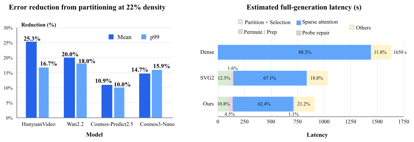
Partition and reconstruction. Table 2 compares partition variants and probe-fitted reconstruction. The key-response K/V variant changes only the K/V partition, while the response-coupled variant also derives the query partition from K/V centroids. For repair comparisons, probe indices and estimator settings are fixed, and errors are reported only on unprobed rows. Response-coupled partitioning reduces both mean and p99 error relative to semantic partitioning on all four models. Probe fitting provides the larger reduction, and benefits more from the response-coupled partition. Figure 4(a) summarizes the fixed-density comparison.

Table 2: Partition and Reconstruction ablation at matched routed-pair density. Entries report mean/p99 normalized attention-output error; lower is better.

Configuration	HunyuanVideo	Wan2.2	Cosmos- Predict2.5	Cosmos3-Nano
Partition construction, repair disabled
Semantic partition	0.0887 / 0.7136	0.1634 / 1.7338	0.7903 / 7.5318	0.3590 / 3.3557
Key-response K/V partition	0.0851 / 0.8121	0.1560 / 1.6591	0.7686 / 7.2700	0.3409 / 3.1738
Response-coupled partition	0.0736 / 0.6967	0.1489 / 1.6479	0.7617 / 7.2271	0.3315 / 3.1502
Partition–repair interaction
Semantic partition + probe repair	0.0527 / 0.3562	0.1041 / 0.8186	0.2622 / 0.8260	0.1720 / 0.8648
SparsePR	0.0330 / 0.2285	0.0707 / 0.4305	0.0954 / 0.5769	0.0822 / 0.4951

Density sweep. Table 3 evaluates Cosmos3-Nano across five executed-pair budgets. SparsePR achieves lowest mean and p99 error at every density, showing gains across operating points.

Table 3: Cosmos3-Nano sensitivity to total executed-pair density

\rho

. Entries report mean/p99.

Method $\bm{\rho=12\%}$ $\bm{\rho=17\%}$ $\bm{\rho=22\%}$ $\bm{\rho=28\%}$ $\bm{\rho=35\%}$ Semantic + hard drop 0.5469 / 4.9925 0.4347 / 4.0098 0.3590 / 3.3557 0.2929 / 2.7780 0.2354 / 2.2662 Response-coupled + hard drop 0.5061 / 4.6345 0.4016 / 3.7486 0.3315 / 3.1502 0.2701 / 2.6168 0.2170 / 2.1421 Semantic + probe repair 0.1484 / 0.8377 0.1140 / 0.6680 0.1720 / 0.8648 0.0764 / 0.4835 0.0627 / 0.4183 SparsePR 0.1274 / 0.7245 0.0990 / 0.5771 0.0822 / 0.4951 0.0681 / 0.4222 0.0567 / 0.3669

Probe and estimator design. With response-coupled partitioning fixed, Table 4 compares probe selection and output-subspace regularization. Query-group-stratified probes achieve lowest mean and p99 error. Probe-residual subspace projection provides a small consistent gain over ridge alone.

Table 4: Probe-selection and estimator ablations with the response partitiotn,

M=64

r=16

Configuration	HunyuanVideo	Wan2.2	Cosmos- Predict2.5	Cosmos3-Nano
Probe selection
Random probes	0.0382 / 0.2361	0.0775 / 0.4533	0.0977 / 0.5873	0.0852 / 0.5024
Uniform spatiotemporal probes	0.0402 / 0.2486	0.0820 / 0.4316	0.1068 / 0.6283	0.0898 / 0.5359
Query-group-stratified probes	0.0329 / 0.2271	0.0708 / 0.4307	0.0953 / 0.5768	0.0818 / 0.4907
Estimator design with query-group-stratified probes
Ridge only	0.0340 / 0.2332	0.0734 / 0.4530	0.0995 / 0.5882	0.0837 / 0.5041
Ridge + probe-residual subspace	0.0329 / 0.2271	0.0708 / 0.4307	0.0953 / 0.5768	0.0818 / 0.4907

5.3 Runtime Analysis

Figure 4(b) decomposes estimated full-generation latency on Wan2.2. SparsePR reduces latency from $1650$ s to $917$ s, corresponding to a $1.80\times$ speedup, compared with $1038$ s and $1.59\times$ for SVG2. Probe-Fitted Residual Reconstruction accounts for only $1.1\%$ of latency. Thus, the primary fidelity gain from probe fitting adds little end-to-end overhead.

Acknowledgments

This work used ACES at Texas A&M University through allocation CIS250376 from the Advanced Cyberinfrastructure Coordination Ecosystem: Services & Support (ACCESS) program, which is supported by U.S. National Science Foundation grants #2138259, #2138286, #2138307, #2137603, and #2138296 1.

6 Conclusion

We studied training-free block-sparse attention as an executable operator in which partitioning shapes both shared support and the residual left by skipped interactions. SparsePR addresses these effects with Response-Coupled Partitioning and Probe-Fitted Residual Reconstruction, combining response-based grouping with call-specific residual correction. Across four video generation and world models, SparsePR reduces attention-reconstruction error, with probe fitting providing the largest fidelity gain and response-coupled partitioning further improving reconstruction. SparsePR closely matches dense benchmark quality while achieving $1.48\times$ to $2.61\times$ end-to-end speedups at 22% to 26% realized executed-pair density. These results show that effective sparse execution depends on both partition geometry and reconstruction of skipped interactions.

References

Boerner et al. (2023) T. J. Boerner, S. Deems, T. R. Furlani, S. L. Knuth, and J. Towns ACCESS: advancing innovation: NSF’s advanced cyberinfrastructure coordination ecosystem: services & support. In Practice and Experience in Advanced Research Computing (PEARC ’23), pp. 173–176. External Links: Document Cited by: Acknowledgments.
Chen et al. (2021) B. Chen, T. Dao, E. Winsor, Z. Song, A. Rudra, and C. Ré Scatterbrain: unifying sparse and low-rank attention. Advances in Neural Information Processing Systems 34, pp. 17413–17426. Cited by: §2.
Chen et al. (2026a) P. Chen, X. Zeng, M. Zhao, M. Shen, W. Cheng, G. Yu, and T. Chen Sparse-vdit: unleashing the power of sparse attention to accelerate video diffusion transformers. In Proceedings of the AAAI Conference on Artificial Intelligence, Vol. 40, pp. 2957–2965. Cited by: §1, §2.
Chen et al. (2026b) R. Chen, K. Mills, L. Jiang, C. Gao, and D. Niu Re-ttention: ultra sparse visual generation via attention statistical reshape. Advances in Neural Information Processing Systems 38, pp. 58029–58055. Cited by: §2.
Choromanski et al. (2020) K. Choromanski, V. Likhosherstov, D. Dohan, X. Song, A. Gane, T. Sarlos, P. Hawkins, J. Davis, A. Mohiuddin, L. Kaiser, et al. Rethinking attention with performers. arXiv preprint arXiv:2009.14794. Cited by: §2.
Dao et al. (2022) T. Dao, D. Fu, S. Ermon, A. Rudra, and C. Ré Flashattention: fast and memory-efficient exact attention with io-awareness. Advances in neural information processing systems 35, pp. 16344–16359. Cited by: §2.
Daras et al. (2020) G. Daras, N. Kitaev, A. Odena, and A. G. Dimakis Smyrf-efficient attention using asymmetric clustering. Advances in Neural Information Processing Systems 33, pp. 6476–6489. Cited by: §2.
Glorian et al. (2026) G. Glorian, I. Lamprou, Z. Zhang, Y. Yuan, and H. Liu LVSA: training-free sparse attention for long video diffusion. arXiv preprint arXiv:2605.31057. Cited by: §2.
Han et al. (2026) S. Han, H. Yang, X. Hu, X. Mei, Y. Jiang, and X. Qi Veda: scalable video diffusion via distilled sparse attention. arXiv preprint arXiv:2605.30325. Cited by: §2.
Hu et al. (2026) J. Hu, Z. Gao, Y. He, and K. Yuan DFSAttn: dynamic fine-grained sparse attention for efficient video generation. arXiv preprint arXiv:2605.23445. Cited by: §2.
Huang et al. (2025) Z. Huang, F. Zhang, X. Xu, Y. He, J. Yu, Z. Dong, Q. Ma, N. Chanpaisit, C. Si, Y. Jiang, et al. Vbench++: comprehensive and versatile benchmark suite for video generative models. IEEE Transactions on Pattern Analysis and Machine Intelligence. Cited by: §5.
Kitaev et al. (2020) N. Kitaev, Ł. Kaiser, and A. Levskaya Reformer: the efficient transformer. arXiv preprint arXiv:2001.04451. Cited by: §2.
Kong et al. (2024) W. Kong, Q. Tian, Z. Zhang, R. Min, et al. HunyuanVideo: a systematic framework for large video generative models. arXiv preprint arXiv:2412.03603. Cited by: §1.
Li et al. (2026a) H. Li, Y. Li, J. Chen, T. Ye, H. Liu, J. Yu, D. Wang, R. Zhang, Z. Xie, E. Xie, et al. Sol-attn: accelerating video generation inference via on-the-fly attention sparsification. arXiv preprint arXiv:2607.24027. Cited by: §1, §2.
Li et al. (2026b) H. Li, S. Shao, W. Zhong, Z. Zhou, L. Bai, H. Xiong, and Z. Xie Pisa: piecewise sparse attention is wiser for efficient diffusion transformers. arXiv preprint arXiv:2602.01077. Cited by: §1, §1, §2.
Li et al. (2025) X. Li, Y. Gu, X. Lin, W. Wang, and B. Zhuang PSA: pyramid sparse attention for efficient video understanding and generation. arXiv preprint arXiv:2512.04025. Cited by: §2.
Li et al. (2026c) X. Li, M. Li, T. Cai, H. Xi, S. Yang, Y. Lin, L. Zhang, S. Yang, J. Hu, K. Peng, et al. Radial attention: $O(n\log n)$ sparse attention with energy decay for long video generation. Advances in Neural Information Processing Systems 38, pp. 16822–16852. Cited by: §2.
Liu et al. (2025) X. Liu, Z. Li, J. Zhang, M. Chen, and Q. Gu Rectified spaattn: revisiting attention sparsity for efficient video generation. arXiv preprint arXiv:2511.19835. Cited by: §2.
Luo et al. (2026) J. Luo, J. Chen, J. Wang, C. Wang, H. Zhu, Q. Sun, C. Gao, Z. Chen, and J. Li Attention sparsity is input-stable: training-free sparse attention for video generation via offline sparsity profiling and online qk co-clustering. arXiv preprint arXiv:2603.18636. Cited by: §1, §1, §2, Table 1, Table 1, Table 1, Table 1.
NVIDIA (2025a) NVIDIA PBench: a physical ai benchmark for world models. External Links: Link Cited by: §5.
NVIDIA (2025b) NVIDIA World simulation with video foundation models for physical ai. arXiv preprint arXiv:2511.00062. Cited by: §1.
NVIDIA (2026) NVIDIA Cosmos 3: omnimodal world models for physical ai. arXiv preprint arXiv:2606.02800. External Links: Link Cited by: §1.
Roy et al. (2021) A. Roy, M. Saffar, A. Vaswani, and D. Grangier Efficient content-based sparse attention with routing transformers. Transactions of the Association for Computational Linguistics 9, pp. 53–68. Cited by: §2.
Samuel et al. (2026) D. Samuel, I. Tzachor, M. Levy, M. Green, G. Chechik, and R. Ben-Ari Fast autoregressive video diffusion and world models with temporal cache compression and sparse attention. arXiv preprint arXiv:2602.01801. Cited by: §2.
Shen et al. (2025) X. Shen, C. Han, Y. Zhou, Y. Xie, Y. Gong, Q. Wang, Y. Wang, Y. Wang, P. Zhao, and J. Gu Draftattention: fast video diffusion via low-resolution attention guidance. arXiv preprint arXiv:2505.14708. Cited by: §2.
Sun et al. (2026) W. Sun, R. Tu, Y. Ding, J. Liao, Z. Jin, S. Liu, and D. Tao Vorta: efficient video diffusion via routing sparse attention. Advances in Neural Information Processing Systems 38, pp. 7837–7863. Cited by: §1, §2.
Tan et al. (2026) H. Tan, S. Wang, Y. Qiao, J. Zhang, Y. Bai, P. Gong, Z. Jin, and C. Li AdaCluster: adaptive query-key clustering for sparse attention in video generation. In Proceedings of the IEEE/CVF Conference on Computer Vision and Pattern Recognition, pp. 43249–43259. Cited by: §2.
Tay et al. (2020) Y. Tay, D. Bahri, L. Yang, D. Metzler, and D. Juan Sparse sinkhorn attention. In International conference on machine learning, pp. 9438–9447. Cited by: §2.
Vyas et al. (2020) A. Vyas, A. Katharopoulos, and F. Fleuret Fast transformers with clustered attention. Advances in Neural Information Processing Systems 33, pp. 21665–21674. Cited by: §2.
Wan et al. (2025) T. Wan, A. Wang, B. Ai, B. Wen, C. Mao, C. Xie, D. Chen, F. Yu, H. Zhao, J. Yang, J. Zeng, J. Wang, J. Zhang, J. Zhou, J. Wang, J. Chen, K. Zhu, K. Zhao, K. Yan, L. Huang, M. Feng, N. Zhang, P. Li, P. Wu, R. Chu, R. Feng, S. Zhang, S. Sun, T. Fang, T. Wang, T. Gui, T. Weng, T. Shen, W. Lin, W. Wang, W. Wang, W. Zhou, W. Wang, W. Shen, W. Yu, X. Shi, X. Huang, X. Xu, Y. Kou, Y. Lv, Y. Li, Y. Liu, Y. Wang, Y. Zhang, Y. Huang, Y. Li, Y. Wu, Y. Liu, Y. Pan, Y. Zheng, Y. Hong, Y. Shi, Y. Feng, Z. Jiang, Z. Han, Z. Wu, and Z. Liu Wan: open and advanced large-scale video generative models. arXiv preprint arXiv:2503.20314. Cited by: §1.
Wu et al. (2025) J. Wu, L. Hou, H. Yang, X. Tao, Y. Tian, P. Wan, D. Zhang, and Y. Tong Vmoba: mixture-of-block attention for video diffusion models. arXiv preprint arXiv:2506.23858. Cited by: §2.
Xi et al. (2025) H. Xi, S. Yang, Y. Zhao, C. Xu, M. Li, X. Li, Y. Lin, H. Cai, J. Zhang, D. Li, et al. Sparse videogen: accelerating video diffusion transformers with spatial-temporal sparsity. arXiv preprint arXiv:2502.01776. Cited by: §1, §2.
Xia et al. (2025) Y. Xia, S. Ling, F. Fu, Y. Wang, H. Li, X. Xiao, and B. Cui Training-free and adaptive sparse attention for efficient long video generation. In Proceedings of the IEEE/CVF International Conference on Computer Vision, pp. 15982–15993. Cited by: §1, §2.
Xiong et al. (2021) Y. Xiong, Z. Zeng, R. Chakraborty, M. Tan, G. Fung, Y. Li, and V. Singh Nyströmformer: a nyström-based algorithm for approximating self-attention. In Proceedings of the AAAI conference on artificial intelligence, Vol. 35, pp. 14138–14148. Cited by: §2.
Xu et al. (2025) R. Xu, G. Xiao, H. Huang, J. Guo, and S. Han Xattention: block sparse attention with antidiagonal scoring. arXiv preprint arXiv:2503.16428. Cited by: §1, §2.
Yang et al. (2026) S. Yang, H. Xi, Y. Zhao, M. Li, J. Zhang, H. Cai, Y. Lin, X. Li, C. Xu, K. Peng, et al. Sparse videogen2: accelerate video generation with sparse attention via semantic-aware permutation. Advances in Neural Information Processing Systems 38, pp. 96965–96991. Cited by: §1, §2, §3.1, Table 1, Table 1, Table 1, Table 1.
Yang et al. (2024) Z. Yang, J. Teng, W. Zheng, M. Ding, S. Huang, J. Xu, Y. Yang, W. Hong, X. Zhang, G. Feng, et al. CogVideoX: text-to-video diffusion models with an expert transformer. arXiv preprint arXiv:2408.06072. Cited by: §1.
Ye et al. (2025) Z. Ye, L. Chen, R. Lai, W. Lin, Y. Zhang, S. Wang, T. Chen, B. Kasikci, V. Grover, A. Krishnamurthy, et al. Flashinfer: efficient and customizable attention engine for llm inference serving. Proceedings of Machine Learning and Systems 7. Cited by: §4.3.
Zhang et al. (2025a) J. Zhang, C. Xiang, H. Huang, J. Wei, H. Xi, J. Zhu, and J. Chen Spargeattention: accurate and training-free sparse attention accelerating any model inference. arXiv preprint arXiv:2502.18137. Cited by: §1, §2, Table 1, Table 1.
Zhang et al. (2026) P. Zhang, Y. Chen, H. Huang, W. Lin, Z. Liu, I. Stoica, E. Xing, and H. Zhang Faster video diffusion with trainable sparse attention. Advances in Neural Information Processing Systems 38, pp. 152509–152534. Cited by: §2.
Zhang et al. (2025b) P. Zhang, Y. Chen, R. Su, H. Ding, I. Stoica, Z. Liu, and H. Zhang Fast video generation with sliding tile attention. arXiv preprint arXiv:2502.04507. Cited by: §1, §2.
Zheng et al. (2026) X. Zheng, Y. Ma, J. Xu, X. Zheng, R. Ji, and F. Chao HASTE: training-free video diffusion acceleration via head-wise adaptive sparse attention. arXiv preprint arXiv:2605.14513. Cited by: §2.
Zhou et al. (2026a) R. Zhou, X. Wu, K. He, G. Han, B. Liu, Q. Chen, W. Xu, Q. Zhao, and C. Song ScalingAttention: discovering intrinsic sparse attention topology for video diffusion transformers. arXiv preprint arXiv:2606.23019. Cited by: §2.
Zhou et al. (2026b) X. Zhou, Q. Mang, S. Yang, H. Xi, J. Zhang, H. Mao, J. E. Gonzalez, K. Keutzer, I. Stoica, and A. Cheung SVG-ear: parameter-free linear compensation for sparse video generation via error-aware routing. arXiv preprint arXiv:2603.08982. Cited by: §1, §1, §2, Table 1, Table 1, Table 1, Table 1.

Appendix A Probe-Fitted Residual Reconstruction Details

This appendix derives the exact hard-drop residual and details the call-specific estimator used by Probe-Fitted Residual Reconstruction. The final estimator uses only the sparse output as its regression feature. Query-response coordinates are used for query partitioning and probe selection, but not for residual regression.

A.1 Hard-Drop Residual and Affine Model

For one query row $i$ , let $\mathcal{S}_{i}$ and $\mathcal{U}_{i}$ denote its retained and omitted key-index sets. Define the attention logit

\ell_{ij}=\frac{q_{i}^{\top}k_{j}}{\sqrt{d}}.

(A.1)

The retained and omitted partition sums and value numerators are

	$\displaystyle Z_{S,i}$	$\displaystyle=\sum_{j\in\mathcal{S}_{i}}\exp(\ell_{ij}),$	$\displaystyle N_{S,i}$	$\displaystyle=\sum_{j\in\mathcal{S}_{i}}\exp(\ell_{ij})v_{j},$
	$\displaystyle Z_{U,i}$	$\displaystyle=\sum_{j\in\mathcal{U}_{i}}\exp(\ell_{ij}),$	$\displaystyle N_{U,i}$	$\displaystyle=\sum_{j\in\mathcal{U}_{i}}\exp(\ell_{ij})v_{j}.$		(A.2)

Dense attention and renormalized hard drop therefore compute

O_{i}^{\mathrm{dense}}=\frac{N_{S,i}+N_{U,i}}{Z_{S,i}+Z_{U,i}},\qquad O_{i}^{\mathrm{sp}}=\frac{N_{S,i}}{Z_{S,i}}.

(A.3)

Let

p_{U,i}=\frac{Z_{U,i}}{Z_{S,i}+Z_{U,i}},\qquad O_{U,i}=\frac{N_{U,i}}{Z_{U,i}}\quad(p_{U,i}>0)

(A.4)

denote the omitted dense-softmax mass and the output obtained by renormalizing over the omitted support. Then

O_{i}^{\mathrm{dense}}=(1-p_{U,i})O_{i}^{\mathrm{sp}}+p_{U,i}O_{U,i},

(A.5)

and the exact post-softmax residual is

\boxed{R_{i}=O_{i}^{\mathrm{dense}}-O_{i}^{\mathrm{sp}}=p_{U,i}\left(O_{U,i}-O_{i}^{\mathrm{sp}}\right).}

(A.6)

The sparse output is observable during sparse execution, whereas $p_{U,i}$ and $O_{U,i}$ depend on omitted interactions. We therefore fit a call-specific affine model from the sparse output to the measured residual,

x_{i}=O_{i}^{\mathrm{sp}}\in\mathbb{R}^{d_{v}},\qquad R_{i}\approx b+x_{i}B.

(A.7)

This is an empirical local model for one active attention call, not an assumption that the omitted statistics are uniquely determined by $O_{i}^{\mathrm{sp}}$ . The oracle analysis in the main paper measures how much of the residual can be represented by this affine family under different partitions.

A.2 Query-Group-Stratified Exact Probe Selection

The affine map depends on the current input, head, layer, routing pattern, and denoising step. We therefore estimate it from exact rows of the active attention call rather than from an offline dataset. For each query head, we evaluate $M=64\ll N_{q}$ probe rows against all keys. The probe contribution to executed-pair density is $M/N_{q}$ . Across the evaluated sequence lengths, this fraction ranges from $0.054\%$ to $0.145\%$ .

Probe selection uses the query partition and the query-response coordinates from Response-Coupled Partitioning, without inspecting the dense residual. For each nonempty query group $G_{a}^{Q}$ , define

c_{a}=\frac{1}{|G_{a}^{Q}|}\sum_{i\in G_{a}^{Q}}\phi_{Q}(q_{i}),\qquad d_{i}=\left\|\phi_{Q}(q_{i})-c_{a}\right\|_{2}.

(A.8)

Rows within each group are ordered by increasing $d_{i}$ , with ties broken by the original row index. A round-robin traversal first draws from distinct nonempty groups and then takes additional rows from their radial orderings until the probe budget is exhausted.

Algorithm A.1 Query-Group-Stratified Exact Probe Selection

1: Query groups

\mathcal{G}^{Q}

; query-response coordinates

{\phi_{Q}(q_{i})}_{i=1}^{N_{q}}

; probe budget

M

2: Probe set

\mathcal{P}

\mathcal{P}\leftarrow\varnothing

\mathcal{A}\leftarrow{a:,|G_{a}^{Q}|>0}

in deterministic group order

5: for all

a\in\mathcal{A}

c_{a}\leftarrow|G_{a}^{Q}|^{-1}\sum_{i\in G_{a}^{Q}}\phi_{Q}(q_{i})

\pi_{a}\leftarrow\textsc{SortIndicesAscending}({i\in G_{a}^{Q}},,|\phi_{Q}(q_{i})-c_{a}|_{2})

8: end for

t\leftarrow 1

10: while

|\mathcal{P}|<M

11: for all

a\in\mathcal{A}

12: if

t\leq|G_{a}^{Q}|

and

|\mathcal{P}|<M

then

13:

\mathcal{P}\leftarrow\mathcal{P}\cup{\pi_{a}(t)}

14: end if

15: end for

16:

t\leftarrow t+1

17: end while

18: return

\mathcal{P}

For each probe $p\in\mathcal{P}$ , exact attention provides

R_{p}=O_{p}^{\mathrm{dense}}-O_{p}^{\mathrm{sp}}.

(A.9)

The estimator is fitted from the pairs $\{(x_{p},R_{p})\}_{p\in\mathcal{P}}$ .

Group-coverage weights.

Let $m_{a}=|\mathcal{P}\cap G_{a}^{Q}|$ be the number of probes selected from query group $a$ . Each probe $p\in G_{a}^{Q}$ receives weight

w_{p}=\frac{|G_{a}^{Q}|}{m_{a}}.

(A.10)

Thus, $\sum_{p\in\mathcal{P}\cap G_{a}^{Q}}w_{p}=|G_{a}^{Q}|$ , so groups with more selected probes do not receive disproportionate influence. These are deterministic coverage weights, not an importance-sampling correction.

A.3 Weighted Affine Fitting and Probe-Residual Output Subspace

Normalize the coverage weights to unit sum,

\alpha_{p}=\frac{w_{p}}{\sum_{t\in\mathcal{P}}w_{t}}.

(A.11)

The weighted feature and residual means are

\mu_{x}=\sum_{p\in\mathcal{P}}\alpha_{p}x_{p},\qquad\mu_{R}=\sum_{p\in\mathcal{P}}\alpha_{p}R_{p}.

(A.12)

Define the elementwise feature scale

s_{x}=\left[\sum_{p\in\mathcal{P}}\alpha_{p}(x_{p}-\mu_{x})^{\odot 2}+\epsilon\right]^{1/2},

(A.13)

where $\odot 2$ denotes elementwise squaring. The standardized feature and centered residual are

\bar{x}_{p}=(x_{p}-\mu_{x})\oslash s_{x},\qquad\bar{R}_{p}=R_{p}-\mu_{R},

(A.14)

where $\oslash$ denotes elementwise division. Stacking the probe rows gives $\bar{X}_{\mathcal{P}}\in\mathbb{R}^{M\times d_{v}}$ and $\bar{R}_{\mathcal{P}}\in\mathbb{R}^{M\times d_{v}}$ .

For the regression objective, rescale the coverage weights to have unit mean,

\widetilde{w}_{p}=\frac{Mw_{p}}{\sum_{t\in\mathcal{P}}w_{t}},\qquad W=\operatorname{diag}\left(\{\widetilde{w}_{p}\}_{p\in\mathcal{P}}\right).

(A.15)

This preserves their relative values while keeping the scale of the ridge coefficient less dependent on the query count.

Weighted ridge fit.

The centered feature-to-residual map is

B_{\lambda}=\arg\min_{B}\left\|W^{1/2}\left(\bar{R}_{\mathcal{P}}-\bar{X}_{\mathcal{P}}B\right)\right\|_{F}^{2}+\lambda\|B\|_{F}^{2}.

(A.16)

Its closed form is

B_{\lambda}=\left(\bar{X}_{\mathcal{P}}^{\top}W\bar{X}_{\mathcal{P}}+\lambda I\right)^{-1}\bar{X}_{\mathcal{P}}^{\top}W\bar{R}_{\mathcal{P}}.

(A.17)

The implementation solves the regularized normal equations with a linear solver rather than explicitly forming the inverse.

Probe-residual output subspace.

Let $\Psi_{r}\in\mathbb{R}^{d_{v}\times r}$ contain the leading $r$ right singular vectors of the weighted, centered exact probe-residual matrix,

W^{1/2}\bar{R}_{\mathcal{P}}=U_{R}\Sigma_{R}V_{R}^{\top},\qquad\Psi_{r}=(V_{R})_{[:,1:r]}.

(A.18)

This basis is constructed from the measured probe residuals, not from the fitted residuals. It identifies output directions observed in the exact current-call corrections.

For an unprobed row $i$ , define $\bar{x}_{i}=(x_{i}-\mu_{x})\oslash s_{x}$ . Its predicted residual is

\widehat{R}_{i}=\mu_{R}+\bar{x}_{i}B_{\lambda}\Psi_{r}\Psi_{r}^{\top}.

(A.19)

The projector restricts the feature-dependent correction to output directions observed in the probe residuals. It does not assume that the complete post-softmax residual is globally low rank. No correction-norm cap is applied. The final output is

\widehat{O}_{i}=\begin{cases}O_{i}^{\mathrm{dense}},&i\in\mathcal{P},\\[2.84526pt] O_{i}^{\mathrm{sp}}+\widehat{R}_{i},&i\notin\mathcal{P}.\end{cases}

(A.20)

Appendix B Response-Coupled Partitioning and Sparse Execution

B.1 Key-Response Coordinates for Paired K/V Groups

For each K/V head, let $Q_{s}\in\mathbb{R}^{M_{s}\times d}$ contain a deterministic sample of query rows. Define

M_{K}=\frac{1}{M_{s}}Q_{s}^{\top}Q_{s}.

(B.1)

For any two keys $k_{i}$ and $k_{j}$ ,

(k_{i}-k_{j})^{\top}M_{K}(k_{i}-k_{j})=\frac{1}{M_{s}}\left\|Q_{s}(k_{i}-k_{j})\right\|_{2}^{2}.

(B.2)

Thus, the metric compares pre-softmax response profiles under the sampled queries. Let $F_{K}\in\mathbb{R}^{d\times r_{K}}$ contain the leading $r_{K}$ eigendirections of $M_{K}$ , scaled by the square roots of their eigenvalues after the retained eigenvalues are normalized to unit mean. The key-response coordinate is

\phi_{K}(k_{j})=F_{K}^{\top}k_{j}\in\mathbb{R}^{r_{K}}.

(B.3)

Applying $k$ -means to $\phi_{K}(k_{j})$ produces the paired K/V groups. Each value $v_{j}$ inherits the assignment of its paired key $k_{j}$ . Values do not enter the partition feature.

B.2 Query-Response Coordinates from K/V Groups

Let $C_{k}^{+}$ denote the number of nonempty K/V groups. We compute each nonempty group’s centroid in the original key space, subtract the uniform mean over nonempty groups, and stack the centered centroids as $\widetilde{K}\in\mathbb{R}^{C_{k}^{+}\times d}$ . The query-response metric is

M_{Q}=\frac{\widetilde{K}^{\top}\widetilde{K}}{C_{k}^{+}d}.

(B.4)

Let $F_{Q}\in\mathbb{R}^{d\times r_{Q}}$ be obtained from the leading $r_{Q}$ eigendirections of $M_{Q}$ using the same eigenvalue weighting as above. The normalized query-response coordinate is

\phi_{Q}(q_{i})=\frac{F_{Q}^{\top}q_{i}}{\max\!\left(\sqrt{\|F_{Q}^{\top}q_{i}\|_{2}^{2}/r_{Q}},\epsilon\right)}\in\mathbb{R}^{r_{Q}},\qquad\epsilon=10^{-6}.

(B.5)

Only nonempty K/V groups contribute to $M_{Q}$ , and their centered centroids receive equal weight rather than token-count weight. Clustering $\phi_{Q}(q_{i})$ gives the query partition. The same coordinates are used to stratify probe selection, but not as residual-regression features. Together, the K/V and query stages form a coupled, single-pass construction without alternating refinement between the two partitions.

Appendix C Implementation and Evaluation Details

C.1 GPU Implementation

The implementation uses warm-started GPU $k$ -means and a fused query-response projection and RMS-normalization kernel. At the evaluated production shape, the fused query projection reduces latency from $1.6170$ ms to $0.5064$ ms and has relative feature error $3.68\times 10^{-4}$ against the reference implementation. Residual fitting, probe-residual SVD, projection, and correction are implemented with small batched GPU linear-algebra operations.

C.2 Shared Hyperparameters

All experiments use BF16 on a single NVIDIA H100 GPU. The method settings are shared across models except for the selected total executed-pair target.

Table C.1: Method configuration used in the evaluated models.

Parameter	Value
Key-response rank $r_{K}$	$48$
Query-response rank $r_{Q}$	$64$
Exact probes per query head $M$	$64$
Probe-residual output rank $r$	$16$
Ridge coefficient $\lambda$	$0.1$
Target $\rho_{\mathrm{exec}}$ for HunyuanVideo, Wan2.2, Cosmos-Predict2.5	$0.22$
Target $\rho_{\mathrm{exec}}$ for Cosmos3-Nano	$0.26$

Table C.2: Probe-row fractions for the evaluated sequence lengths with

M=64

Model	$\bm{N_{q}}$	$\bm{M/N_{q}}$
HunyuanVideo	$118{,}800$	$0.054\%$
Wan2.2	$75{,}600$	$0.085\%$
Cosmos-Predict2.5	$84{,}480$	$0.076\%$
Cosmos3-Nano	$44{,}160$	$0.145\%$

C.3 Timing Protocol

Dense and sparse runs use matched checkpoints, conditioning inputs, random seeds, sampling schedules, inference steps, guidance settings, resolutions, and frame counts. Executed-pair density counts exact query–key interactions, including probe rows. Reported latency also includes response-coordinate construction, clustering, routing, permutation, sparse attention, exact probes, residual fitting, correction, and output restoration.

Appendix D Cross-Model Density Sensitivity

Figure D.1 compares semantic and response-coupled partitioning across total executed-pair densities from $12\%$ to $35\%$ , under the same residual-repair configuration. Response-coupled partitioning reduces mean error across all densities and models, with p99 error also reduced over nearly the full range. The gains persist across operating points, showing that the partitioning benefit is not specific to a single density.

Figure D.1: Cross-model density sensitivity. Mean (top) and p99 (bottom) normalized attention-output error versus total executed-pair density for semantic and response-coupled partitioning under the same residual-repair configuration. The dashed line marks the

22\%

reference density.

Partition the Support, Reconstruct the Residual: Training-Free Sparse Attention for Video Generation and World Models