Quantile Restrictions, Revealed Rankings, and the Limits of Multinomial Choice
Abstract
This paper analyzes when choice probabilities reveal rankings of deterministic utility indices in semiparametric discrete choice models. It begins with binary choice, where quantile thresholds guarantee ranking recovery, and shows that such thresholds can arise either from behavioral departures from utility maximization (e.g., limited attention) under exchangeable unobservables, or from non-exchangeable unobservables under standard utility maximization. These behavioral and distributional routes are then extended to multinomial choice. Under limited attention, balance restrictions on attention probabilities yield global linear ranking partitions which are robust to the distribution of unobservables and, given sufficiently rich joint variation in the differences of utility indices, are also necessary. Absent the required attention restrictions, opposite rankings can produce overlapping probability images. Under non-exchangeable unobservables, a comparable distribution-uniform partition generally need not exist.
Holding the distribution fixed, however, ranking recovery remains possible via an injective nonlinear map from normalized utility differences to choice probabilities under both behavioral and distributional extensions. Together, the results distinguish distribution-robust global ranking partitions from ranking recovery with a fixed distribution of unobservables and clarify the limits of extending binary quantile restrictions to multinomial choice.
- Keywords:
-
Binary choice; Multinomial choice; Quantile restrictions; Probability simplex; Ranking; Ranking ambiguity; Consideration sets; Non-exchangeability
1 Introduction
Semiparametric discrete choice models often obtain identifying content from weak restrictions on the conditional distribution of unobservables rather than from a fully parametric specification. A classic example is the binary response model studied by 15; 16, , together with the conditional median restriction . Under this restriction, observed choice probabilities reveal the sign of the deterministic utility index as in
| (1.1) |
More generally, if , then
| (1.2) |
The econometric content of this representation is well known. Geometrically, in (1.2) a single threshold divides the one-dimensional probability simplex into two regions corresponding to the two possible rankings of the deterministic utilities. That is, once the location of relative to the threshold is known, the ranking is known as well.
This paper analyzes whether an analogous idea can be extended to multinomial choice. With alternatives, the vector of choice probabilities lies in a -dimensional simplex and there is no longer a single probability threshold. I use the term “quantile” multinomial choice to signify the property that a specified probability domain can be partitioned into regions such that membership in a region reveals a unique ranking of the deterministic utility indices. In the strongest results below this domain is the ambient probability simplex itself. In some weaker results, it is the common structural probability image generated by the fixed conditional distribution of unobservables. The “quantile” terminology is not meant to be associated with a conventional multivariate quantile notion.
A weaker property than a full “quantile ” model is ranking recovery when each attainable probability vector has a unique ordinal interpretation, even when the attainable probability set covers only part of the ambient probability domain.
The extension from two to several alternatives is not automatic. With two alternatives, all relevant variation operates along a single comparison. With three or more alternatives, the probability of choosing rather than can also be affected by what happens to other alternatives. As illustrated in the paper, generally probability vectors generated by different rankings of the deterministic indices can overlap. In other words, the same observed probability vector obtained under some and may then be compatible with both and . This failure of ordinal recovery can be understood as ranking ambiguity. One of the central questions of this paper is what restrictions on the decision making or on the distribution of utility unobservables prevent such ambiguity.
I approach this question by first returning to the binary model and asking what economic structures can generate the quantile representation (1.2). In the classical random utility interpretation underlying the median model, agents maximize latent utility and the two utility unobservables are conditionally exchangeable.11 1 Original 14 restriction was conditional i.i.d. but 10 and later 8 note that conditional exchangeability suffices for the rank order result. In binary choice, exchangeability also implies a zero median of the error difference. Most semiparametric work takes the median or quantile restriction as a primitive. I look into rationalizing quantile restrictions in discrete choice models along two different routes. Either of them can generate representation (1.2). A behavioral route maintains conditional exchangeability of the latent utility unobservables but allows decision making to differ from utility maximization. The decision rule may reflect limited consideration, noisy perception, or other stochastic behavior. A distributional route maintains standard utility maximization but allows the joint distribution of the utility unobservables to be non-exchangeable.
I then carry these two routes into multinomial choice. The natural benchmark is the classical random utility model of 14. Under utility maximization with conditionally i.i.d. unobservables and some further standard 14 conditions,
| (1.3) |
which I will refer to as Manski’s rank order property. Pairwise equalities of choice probabilities, therefore, describe hyperplanes that split the probability simplex into regions corresponding to unique complete rankings of the deterministic utility indices. I use this classical case as the multinomial “median” benchmark and ask how much of its ranking geometry survives under limited attention and under non-exchangeable unobservables in latent utilities.
The paper makes three main substantive contributions and develops a framework for distinguishing the robustness of the resulting ranking claims.
The first main contribution is to give economic foundations for binary non-median (and median as a special case) probability thresholds. In line with the behavioral route mentioned above, I describe general stochastic decision rules that give (1.2) under conditionally exchangeable unobservables and go beyond standard utility maximization. These include limited attention, noisy perception, and random choice, with exogenous consideration sets providing a particularly transparent foundation for both median and non-median cases. For the second distributional route, I show how non-median thresholds can instead arise from asymmetry in the joint distribution of latent utility unobservables with agents still maximizing utility.
The second main contribution is to study ranking recovery and stronger “quantile” partitionings in multinomial models and to do so at different levels capturing different robustness properties. A Behavioral environment level specifies a decision rule and an admissible class of conditional distributions of unobservables. A Structural environment additionally fixes one such conditional distribution.33 3 The main text also mentions an empirical specification level, which also fixes the marginal distribution of the covariates, but does not study findings at this level as it requires a case-by-case analysis. In addition to these two levels, the paper also studies which results apply for a fixed or uniformly over all admissible .
The sharpest results arise in the behavioral route when looking at the exogenous consideration sets. Limited attention changes the geometry of the probability simplex since choice probabilities now combine utility comparisons across different menus. Nevertheless, particular restrictions on attention probabilities can restore linear pairwise ranking rules, generalizing 14 partitioning. These are restrictive balancing conditions on attention probabilities and they become increasingly more restrictive as increases. When these conditions are satisfied, the conclusions are strong as the partitioning is not only (i) linear, (ii) fully determined by attention probabilities and (iii) applies to any absolutely continuous conditionally exchangeable distribution of unobservables, but is also (iv) uniform over the admissible index parameters . Thus, this is the case when ‘‘quantile’’ multinomial choice is obtained, which in particular implies the ranking recovery property for attainable probabilities. But when the balancing conditions on attention probabilities fail, the probability images of opposite pairwise rankings can overlap, producing ranking ambiguity. To my knowledge, this paper provides the first characterization of the exogenous attention structures that support distribution-robust linear ordinal recovery that includes asymmetric structures generating nonstandard probability boundaries,44 4 That is, different from 14 boundaries . together with corresponding necessity and failure results.
The distributional route gives a different conclusion. If the conditional distribution of the utility unobservables is allowed to vary over an admissible class of absolutely continuous, potentially non-exchangeable distributions, there is in general no probability partition that is common across that class.
The third main contribution is to show that ranking recovery and “quantile” partitionings can be restored under weaker robustness requirements of the Structural environment level. In both the limited attention model and the model with non-exchangeable unobservables, a common location-scale structure induces a map from normalized deterministic utility index differences into choice probabilities. Under the conditions developed in the paper, this map is injective, so the probabilities again identify the ranking of the deterministic utility indices, ensuring ranking recovery property on the attainable set of probability vectors. The map is generally nonlinear. Under limited attention it depends on the attention probabilities, while under utility maximization with non-exchangeable unobservables it depends on the fixed distribution of the unobservables. Importantly, it does not depend on the parameter vector . This map is best understood as giving a common structural ranking partition for the given Structural environment. The fact that the map is common to the environment supports an interpretation of this case as Structural environment “quantile” multinomial choice when admissible values of index parameter jointly cover the maximal probability domain permitted by this location-scale structure.
Overall, a “quantile” interpretation of multinomial choice requires enough structure to generate a global ranking partition of the relevant probability domain. Whether that partition is over the ambient simplex and robust to the distribution of unobservables, or whether it is specific to a given Structural environment is a separate robustness question.
There is also a fundamental asymmetry between binary and multinomial cases. In binary choice, behavioral and distributional distortions act on a single margin and a quantile representation can survive under much weaker conditions than an analogous “quantile” representation in multinomial choice.
The paper contributes to several related literatures. It builds directly on the semiparametric discrete choice framework of 14; 15; 16. It is also related to work on binary choice under quantile restrictions. 12 studies smoothed binary regression quantiles, while 21 develops asymptotic theory for binary response quantile processes with linear quantile restrictions. That literature largely takes the quantile restriction as an econometric primitive. This paper instead asks which behavioral and distributional structures can generate the probability threshold and what remains of its ordinal interpretation when choice becomes multinomial. 19 studies nonparametric identification of multinomial choice models with flexible deterministic utility functions and weak distributional restrictions, but preserves the classical pairwise ranking geometry of 14.
The paper is also related to the literature on consideration sets. 8 also studies rank ordering in multinomial choice models with unobserved random consideration sets. His result preserves Manski’s rank order property (1.3) by imposing restrictions on covariate-dependent consideration probabilities that essentially force the consideration mechanism to reinforce the Manski ranking (1.3). In particular, in binary choice his assumptions force the model to preserve the classical Manski median threshold. In contrast, this paper holds attention probabilities fixed and characterizes the balance conditions under which ordinal recovery nevertheless emerges from the attention structure itself, allowing the relevant separators to differ from the standard comparison .
5 develop a discrete choice model with heterogeneous risk preferences and unobserved consideration sets and provide conditions for its identification. In comparing limited consideration with standard random utility models, they introduce a conditional analogue of Manski’s rank order property (1.3) (conditional on latent risk preference type) and show that it implies a generalized dominance restriction on observed choice probabilities, a restriction that limited consideration can violate. An earlier working paper 4 also studies a Random Consideration Level (RCL) model and shows that it preserves the conditional Manski’s rank order property. RCL imposes a strong symmetry restriction, where conditional on consideration set size, all sets are equally likely, so swapping any two alternatives leaves the probability of the consideration set unchanged. This symmetry is a special case of the balance restrictions characterized here. The present paper allows asymmetric attention, characterizes the restrictions under which distribution-robust ordinal recovery remains possible, and derives the resulting—potentially non-Manski linear probability boundaries.
2 shows that, with bounded observable utility shifters, exogenous limited consideration can be observationally equivalent to full consideration, whereas this paper studies when it preserves ordinal recovery directly.
Other relevant consideration sets literature is 18, 17, 6, and 1. The question here is different. Rather than treating consideration probabilities themselves as the principal object to be identified, I take the consideration structure as given and ask what ordinal information about deterministic utilities is encoded in the resulting choice probability geometry. In addition, the object of interest is not a single fixed preference ranking, but the ranking of deterministic utility indices as covariates vary. The relevant variation thus comes from the movement of the choice probabilities across covariate values and from whether the resulting probability images associated with different rankings remain separated. 7 study recovery of cognitive heterogeneity from aggregate choice shares, showing that a single sufficiently large menu can suffice under homogeneous preferences.
Finally, the results at the Structural environment level are related to single-crossing arguments in 3 and 5. Those papers use single-crossing conditions in heterogeneous preferences or types as part of their identification arguments. Here I do not impose a single-crossing ordering of heterogeneous preferences as a primitive. Instead, for a fixed Structural environment, common location-scale restrictions generate a generally multidimensional map from normalized deterministic utility index differences into choice probabilities. Injectivity of this map yields ranking recovery, while the range of attainable normalized indices determines how much of the associated global ranking partition is attained. Thus, both approaches exploit ordinal structure, but in different spaces.
The rest of the paper is organized as follows. Section 2 studies binary choice and develops behavioral and distributional foundations for median and quantile threshold representations. Section 3 turns to multinomial choice, introduces the ranking-recovery framework and the levels of robustness, and studies limited attention and non-exchangeable utility unobservables. Section 4 concludes.
2 Binary choice
A standard starting point, including in 15; 16, for a semiparametric binary choice model is the formulation
with describing the part of utility depending on the observed characteristics and potentially identifiable, whereas describes the unobservable component driving it. The subsequent analysis of such a model relies on what is assumed about the relationship between the unobserved and observed covariates . A canonical restriction of that relationship comes from 15; 16 and relies on imposing the following constraint:
| (2.4) |
This restriction still allows for rich dependencies on from the conditional distribution of while at the same time providing an inferential context on utility indices in terms of observed choice probabilities , which I review in more detail below.
The motivation for the median restriction (2.4) is standard and comes from 14 random utility framework in which each option is associated with a latent utility and the agent chooses the option with the higher utility. In the binary case, let and define latent utilities as , , for . In the standard utility optimization the agent chooses option 1 if and only if Under the assumption that are i.i.d. conditional on , the difference has zero conditional median and the c.d.f of this difference conditional on is strictly increasing in the neighborhood of 0.
In what follows, define , where collects all distinct covariates appearing in or . The associated coefficient vector assigns to each covariate the difference between its coefficients in and , using for absent covariates. Thus, consolidates without redundancy. In particular, if and share no covariates, then , . Conditioning on is therefore informationally equivalent to conditioning on .
Denoting we end up with the model
| (2.5) | ||||
| increasing around 0 | (2.6) |
(2.5)-(2.6) implies that observed choice probabilities are informative about the sign of the utility index in the following sense:
or equivalently, (1.1). Characterization (1.1) underlies both identification arguments and estimation methods in semiparametric binary choice models.
16 proposed a quantile-based semiparametric binary choice model:
| (2.7) |
plus the monotonicity of the conditional c.d.f. analogous to the above, but the quantile index need not equal . Choice probabilities are then informative as (1.2) holds. Behavioral or distributional motivations for (2.7) or (1.2) have received very little attention in the literature.
Remark 1.
Remark 2.
Remark 3.
By the standard random utility paradigm, this paper means a setting in which the agent chooses the option with the highest realized latent utility.
2.1 Behavioral route: General theorem (any )
We start by imposing the following assumption, which permits more general conditional dependence between and than the conditional i.i.d. structure in 14.
ASSUMPTION 1 (Distribution of ).
Suppose the following hold:
- (a)
and are identically distributed conditional on , with absolutely continuous with respect to Lebesgue measure.
- (b)
The copula that describes the dependence between and conditional on is exchangeable (that is, ) and absolutely continuous.
- (c)
The support of the joint distribution of is convex and has a non-empty interior.
Thus, the unobservables may be conditionally correlated, with dependence restricted to exchangeable copulas. This nests the conditional independence copula of 14.
Remark 4.
Throughout, the aim is to derive conditions that are generic, in the sense that they do not rely on particular features of the conditional distribution of the unobservables given , nor on the marginal distribution of or on the value of . This perspective is especially important when discussing necessity.
To that end, the paper abstracts from specifications in which restrictions on the joint support of limit the range of the index relative to the support of . Such cases can be viewed as non-generic, as they can typically be resolved by enriching the model by, for instance, expanding the support of or adjusting so that spans the relevant range of .
The necessity results below are therefore stated for this enriched class, which we call generic models.55 5 In much of the classic literature, the model is effectively specified in this enriched form: has full support on , and varies over with . These assumptions are mainly for analytical convenience and can be relaxed in some settings. In the multinomial models of Section 3, this idea is formalized through different layers of analysis but doing so here would be unnecessarily cumbersome.
The theorem below characterizes the behavioral conditions under which (1.2) holds for any under Assumption 1, while allowing departures from utility maximization. It nests the median specification (1.1) as the special case , again allowing deviations from the standard random utility paradigm.
THEOREM 1 (General theorem for any ).
Let , , and let the distribution of satisfy Assumption 1.
A. The choice behavior of an economic agent can be represented as in (1.2) if the following conditions are satisfied:
- (1)
a.e.;
- (2)
a.e.
Equivalently, Condition (2) can be written as a.e.
B. If the choice behavior of an economic agent can be represented as in (1.2) and condition (2) holds, then Condition (1) is necessary away from index indifference:
| (2.8) |
C. Condition (2) cannot be omitted from the distribution-free sufficiency result in Part A. More precisely, for every and every , there exists a generic model satisfying Assumption 1 and the strict version of Condition (1), but violating Condition (2) on a set of positive measure, for which (1.2) fails.
Condition (1) of Theorem 1 ensures that the agent is more likely to choose option 1 when than when . It rules out choice rules so perverse that higher utility of an option reduces the probability of choosing it. This guarantees the expected monotonic relationship since as the index crosses zero from below, crosses the threshold from below.66 6 This monotonicity condition is distinct from the single-crossing property in random utility models (3). Single-crossing imposes an ordering on preference heterogeneity such that rankings over alternatives change at most once across types, whereas the present condition is a much weaker reduced-form restriction on choice probabilities.
Condition (2) of Theorem 1 relaxes the standard random utility paradigm implication Under Assumption 1, this implication would yield the median condition (2.4). Theorem 1 instead allows choice reversals relative to this benchmark, even when , provided they are independent of which alternative has higher realized utility. For , the theorem gives the first behavioral characterization in the literature of the representation (1.2).77 7 If Condition (2) holds but Condition (1) fails, monotonicity may reverse, yielding the unintended implication .
Part A in Theorem 1 is about sufficiency, whereas parts B and C establish near-necessity. Part B cannot be strengthened to include with . Part C shows that if Condition (1) holds strictly, then violation of Condition (2) generically invalidates (1.2).
Note that Theorem 1 does not require choices to depend only on . Choices may depend on the levels of and as well, provided the theorem’s two conditions hold with examples of such behavioral models given below. Before presenting examples, let’s summarize some implications of model (1.2) on the choice probabilities.
Proposition 1.
Consider the setting in Theorem 1 and suppose conditions (1) and (2) there hold. Then a.e., and
- (i)
for , ;
- (ii)
for , .
Thus, Proposition 1 yields a testable implication: when , the choice probability is bounded strictly away from at least one boundary. This is driven by the fact that under conditions of Proposition 1, In the median model can approach 1 and 0 arbitrarily closely on sets on positive (but decreasing) measure of .
We now give some examples of behavioral models that go beyond the traditional random utility framework while still admitting the representation (1.1) based on Theorem 1.
EXAMPLE 1 (Mixture of random choice and utility maximization, ).
For an economic agent characterized by , with probability , the choice between 1 and 0 is made by tossing a fair coin, and with probability , the choice is made on the basis of comparing latent utilities as in the standard random utility paradigm. Then and . Condition (1) holds since . Condition (2) holds for since and sum to 1.
EXAMPLE 2 (Noisy Perception Model, ).
Suppose an agent does not know their and instead perceives their noisy versions where is independent of conditional on with 88 8 Equivalently, . This is not a strong requirement especially taking into account that centered around 1 would give us the disturbed latent utilities centered around true . ( and can be dependent). Agent’s choice is made by maximizing these noisy versions. Hence, and . Condition (1) in Theorem 1 is guaranteed by . Condition (2) holds too a.e. for as and sum to 1.
2.2 Consideration sets as the canonical behavioral model
As it turns out, models with consideration sets provide the canonical behavioral implementation of Theorem 1 for .
Independent consideration set formation Suppose the collection of possible consideration sets is , with probabilities , , and , respectively. These consideration sets are formed independently of . When the agent faces the set , she chooses the alternative with the higher latent utility. The model can be written as , where and are independent binary random variables, also independent of , with , . Here, indicates that the consideration set is a singleton, while indicates that this singleton is . Thus, independence of and from captures the exogeneity of consideration set formation. Namely, which alternatives enter the consideration set is completely independent of the other variables in the model.
Then and, under Assumption 1,
If then we in fact obtain a model with the median characterization (1.1) which is special case of the model in Example 1. If we obtain a quantile characterization (1.2) for . The asymmetry in consideration probabilities directly controls the quantile index.99 9 An equivalent approach would be to rely on Theorem 1 and show that , and that , which creates a non-median formulation for .
The consideration sets model presented here has testable implications beyond Proposition 1, including when . Namely, , so choice probabilities are bounded away from zero if , from one if , and from both boundaries if both are positive. Since under our maintained conditions, they are always bounded away from at least one boundary. Hence, if lies arbitrarily close to both zero and one with positive probability over , this model is ruled out.
When , we have a.e., and the only consideration sets are and . This case captures a predisposition toward option 1, with measuring its strength. Equivalently, it can represent probabilistic conformity to a social norm being option 1.
There are other models that may result in (1.2) and are in essence similar to the consideration sets models. Example 3 illustrates that.
EXAMPLE 3 (Elements of heuristic decision making).
Suppose an agent’s decision involves evaluation of an aspect in the first step which is independent of in the following way. If is above , then 1 is chosen. If is below , then 0 is chosen. If then the decision is made on the basis of which latent utility is greater.
Let , and . Then
Heterogeneous consideration set formation What if we weakened the assumption on by allowing them to be correlated with but maintained their independence from and from each other given ? Denoting , , we obtain , and under Assumption 1,
Thus, models with heterogeneous consideration set formation (where and depend on ) can also generate (1.2), provided a.e. for some constant . If in this condition , then cannot approach 0 arbitrarily closely as it is bounded away from 0 by , therefore potentially can approach 1 arbitrarily closely but not 0. If , then cannot approach 0 arbitrarily closely (it has to be greater or equal than ) therefore potentially can approach 0 arbitrarily closely but not 1. To summarize, when this heterogeneous choice formation model gives (1.2) model for , it weakens the testable implications of independent consideration set formation. Probabilities now need only be bounded away from one boundary, as in Proposition 1.
The question now is whether there are other foundations that lead to (1.2), particularly those where the choice probabilities could approach both natural probability boundaries 0 and 1 arbitrarily closely for . This is addressed in the next section.
2.3 Distributional route: Non-exchangeable distribution of
We now show that (1.2) can also be rationalized within the standard random utility paradigm by allowing the joint distribution of to be asymmetric. The following theorem covers both non-exchangeable copulas and unequal marginal distributions. Although it allows for behavior beyond the standard random utility model, our main interest is the standard case, where the role of distributional asymmetries in the unobservables is especially transparent.
THEOREM 2.
Let , , and let the joint distribution of be absolutely continuous, have convex support with nonempty interior and let the support of contain in its interior. Then:
A. The choice behavior can be represented as in (1.2) if the following conditions hold:
- (1’)
Condition (1) in Theorem 1 holds;
- (2’)
a.e.
B. If the choice behavior of an economic agent can be represented as in (1.2) and condition (2’) holds, then Condition (1’) is necessary away from index indifference, as in (2.8).
C. Condition (2’) cannot be omitted from the distribution-free sufficiency result in Part A. More precisely, for every fixed , there exists a generic model satisfying the maintained assumptions and the strict version of Condition (1’), but violating Condition (2’) on a set of positive -measure, for which (1.2) fails.
Condition (2’) in Theorem 2 suggests that the covariates and the error dependence interact in a way that stabilizes the threshold for the choice probability. Analogously to Theorem 1, part A is about sufficiency, while parts B and C provide corresponding near-necessity results.
Condition (2’) reduces to Condition (2) when the joint distribution of is exchangeable, since in that case. Under the standard random utility paradigm (, ), Condition (2’) becomes a.e., which is the constancy across of the asymmetry of the joint unobservable distribution. When the marginals of and conditional on are identical (Assumption 1(a) holds) but the copula is not exchangeable, this becomes a.e., that is, the copula must have a fixed degree of asymmetry across . Appendix C shows that this condition is satisfied for an explicit parametric family of absolutely continuous copulas, and that any is attainable.
The key difference of the described distributional route from the behavioral route is that no boundary restriction on emerges as choice probabilities can approach both zero and one, as the copula non-exchangeability can accommodate any probability level.
3 Multinomial choice: More than two options
In the binary case characterization (1.2) effectively described the partitioning of the one-dimensional simplex , more precisely its feasible subset implied by the testable restrictions in Proposition 1. With more than two options, the analysis inevitably becomes substantially richer and more complex. This section studies the extent to which the partition result of the binary case survives under more general behavioral and distributional assumptions.
3.1 Review of 14 multinomial model: “median” multinomial choice
I begin with the classical 14 multinomial choice model. I consider it the “median” benchmark for multinomial choice, as the binary choice model (1.1) under the median threshold arises as its special case.
The latent utility of an agent for the option is
| (3.9) |
On a general note, and not specifically in relation to 14, it is useful to distinguish the support of the covariates from the range of the deterministic utility indices. Even if each has full support, the vector need not span , e.g. when covariates are shared across alternatives. Moreover, since choices and rankings depend only on relative utilities, the relevant richness concerns the index differences rather than the index levels. Sufficient ranking results later in this paper apply on the index configurations that are attainable. This includes the special case in which the index differences range over all of , but does not require it. Additional richness of the joint index difference will be imposed only where it is needed for converse results or for conclusions that require every strict ordering region to be nonempty.
The assumption of i.i.d. of conditional on and the support of being , under the standard random utility paradigm one obtains
| (3.10) |
Relations (3.10) imply that . Note that the full support assumption on the conditional distribution of guarantees that the vector never hits the boundary of the -dimensional simplex :
Without that full support assumption on the distribution of , the utility indices may reach the boundary of the support of the unobservables or even extend beyond it in which case inequality relationships between choice probabilities may become uninformative about the corresponding relationships between the associated utility indices. Therefore, when working under the more general distributional assumptions, it would be natural to reformulate (3.10) by excluding points in the simplex that are obtained when some index differences are either at the boundary or beyond the support of . This will be done in a technically proper way later in our discussion. For now, for expositional simplicity let us maintain that full support condition.
There are some observations worth noting here. We can define preference relations over the choice set either in terms of probabilities,
or in terms of indices,
These two preference relations are equivalent. Moreover, they satisfy the standard axioms of preference relations, including reflexivity, completeness and transitivity.
Another implication of that is that we can create an ordering of the whole list of options by utilizing pairwise relations described above. Namely, take any permutation of . Then
| (3.11) |
iff
| (3.12) |
The following theorem essentially shows that (3.10) is consistent with a much wider class of decision rules than standard utility maximization. Before that, let’s formulate an assumption on unobservables.
ASSUMPTION 2 (Distribution of ).
The joint distribution is exchangeable and absolutely continuous and has a convex support on with a non-empty interior.
In Theorem 3 below the maximum of latent utilities , , is denoted as .
THEOREM 3.
This theorem contains a modified version of (3.10). This modification is needed to deal with the case of both and being outside the interior of the support of and, thus, is only relevant when such support is bounded in some directions. For brevity and also due to multiplicity of options, I do not focus on near-necessity formulations (analogous to B and C in theorems 1 and 2).
14 is a special case of Theorem 3 where the joint conditional copula is the independence copula and , , , a.e.
Example 4 below is that of multinomial choice models that satisfy the sufficient conditions of Theorem 3 but go beyond the standard random utility paradigm.
EXAMPLE 4.
Throughout these examples, we will denote .
1. Mistakes in the implementation. With probability , the agent correctly chooses the utility-maximizing option, otherwise she randomizes uniformly over the nonmaximizing alternatives. This model allows for mistakes in implementation even when the agent correctly identifies the utility-maximizing alternative.
Conditions (1)-(3) of Theorem 3 are satisfied as , while for any , we have . Condition 1 holds because and, hence, .
2. Random shortlist around the utility maximizer. Suppose the agent identifies the utility-maximizing alternative and forms a shortlist of fixed size that always contains that alternative. The remaining members are drawn uniformly without replacement from the other alternatives. The agent then chooses uniformly from the shortlist. If , then . If instead for some , alternative enters the shortlist with probability , and hence . Conditions (2) and (3) of Theorem 3 therefore hold, while Condition (1) follows from
3.2 Geometric structure of the “median” multinomial model
To make progress on what we can consider a “quantile” multinomial choice model, we give a geometric interpretation of the 14 model reviewed in Section 3.1 as we associate it with a “median” benchmark for multinomial choice.
Since in 14 an individual always makes a choice, the vector of choice probabilities lies in the -dimensional simplex , as already mentioned above. The geometry of (3.10) is striking.
First, under total indifference
| (3.13) |
in the index space, such an index collection is mapped by the model to the barycentre , as implied by exchangeability in Assumption 2.
Under pairwise indifference
| (3.14) |
model (3.10) implies . Pairwise indifference therefore maps into the hyperplane in . Taken across all pairs, these hyperplanes partition into regions corresponding to the possible complete strict rankings of the indices. The attainable probability set inherits the corresponding regions, although some may be empty. All regions are attained only when the index differences vary sufficiently richly. The regions are pointed convex cones emanating from , truncated at the simplex boundary (Figure 1 for ). Each of the 6 regions in Figure 1 corresponds to one of the possible six preference relations on the whole set of options according to (3.11)-(3.12). For example, the region of the simplex formed by , corresponds to the case either in the index ordering of probability ordering . This region has a common -dimensional border with the region corresponding to and the region corresponding to . The fact that the simplex is partitioned into six regions non-overlapping in their interior is tantamount to transitivity and completeness properties of the preferences defined through on the set of three options.
In the general case of options, each of regions collects all choice probabilities that can arise under a complete ordering for a permutation of elements in . Each such region shares a -dimensional boundary with exactly neighboring regions, obtained by swapping the order of two adjacent elements in the sequence while holding all other orderings fixed. This partition is what we call the “median” benchmark. A more general “quantile” version is a different global ranking partition of the ambient space, with a shifted reference point and possibly non-hyperplanar boundaries.

3.3 Two levels of analysis. Notation and preliminaries
The analysis is conducted at two levels, which differ in what is held fixed and what is allowed to vary. Let denote the admissible, normalized parameter space for .
A Behavioral environment, denoted by , specifies a decision rule, such as standard random utility or a consideration set model with given attention probabilities, and an admissible class of conditional distributions of given . Results at this level are uniform over the conditional distribution of unobservables in . A Structural environment, denoted by , further fixes a conditional distribution . It can therefore be written as . The conditional distribution of is specified for every , where is the effective dimension of (thus, if e.g. the same covariate enters several indices, it appears only once in , and perfect linear combinations can be dealt with analogously). This allows conclusions that are not driven by restrictions on the covariate domain.1010 10 This echoes the paper’s discussion of enriched support in the binary choice case. At the Structural environment level, the support of has already been maximally enriched. The class may be defined by imposing suitable restrictions on these conditional distributions (analogously to 14).
In principle, one could consider an empirical specification level, which further fixes the marginal distribution of and is characterized by .1111 11 If the support of is smaller than , some of the conditional distributions specified by are not used by the empirical specification. I don’t consider this level theoretically as it needs to be approached on a case-by-case basis.
For any , I call a fixed- behavioral specification, and a fixed- structural model. The scope of results with respect to is a separate matter. A behavioral specification level or structural model result may hold e.g. for a fixed , or generically over , or uniformly over . Uniformity over is particularly attractive as it means that the same probability based ranking implication applies for every . This is stronger than establishing, separately for each , a ranking implication that may depend on the particular parameter value.
The result of 14 is at the Behavioral environment level and has the uniformity-in- scope. Given that in empirical practice is not known, the uniform-in- results may therefore prove most valuable for parameter identification.1212 12 If the deterministic component of latent utility were by a more general function rather than , the analogous distinction would be between a behavioral environment that leaves unspecified and a behavioral specification that fixes those functions. Uniformity over the deterministic utility functions would then require the same probability based ranking implication to hold throughout the admissible class of such functions. Section 2 results for binary choice are also at the Behavioral environment level and uniform in .
Simplex subsets of interest. Fix a structural environment and a parameter value . For the fixed- structural model , let denote the conditional choice-probability vector generated at . To simplify notation, we suppress the dependence of on and whenever the fixed structural model is clear from context.
Define the fixed- feasible probability set at the Structural environment level by . Thus, is the closure of the set of probability vectors attainable under as the covariates vary over the full covariate domain. The ultimate feasible probability set associated with the structural environment , allowing the preference parameter to vary, is This union collects the probability vectors attainable for at least one admissible value of .
We can define the corresponding objects at the behavioral specification level with aggregating feasible probability vectors across all conditional distributions of unobservables admitted by , while holding fixed. The corresponding ultimate feasible set is .
Under some behavioral environments, the sets , , , may have affine dimension strictly smaller than , even when the conditional support of is convex and has nonempty interior in . It will be clarified later in the paper under what conditions the relevant feasible set has full affine dimension.
Images of pairwise ordered utility indices. I study whether an observed probability vector (unambiguously) reveals the ordering of the underlying deterministic utility indices. Since this question can be posed either conditionally on a fixed value of or uniformly across values of , the corresponding image sets need to be defined separately.
For any with , and for any fixed- structural model , define
| (3.15) |
| (3.16) |
Thus, collects the choice probability vectors generated under the fixed- structural model when , whereas collects those generated under pairwise index indifference. When is allowed to vary within the structural environment , define the ultimate ordering and indifference images by and , respectively.
For a behavioral specification level for a fixed , define , . These sets aggregate the fixed- ordering and indifference images across all structural models admitted by . When is allowed to vary within , define the ultimate behavioral specification images by , .
Support of unobservables and relative interiors. If the 14 setting has as the support of , and the index differences range over all of , then every probability vector in is attainable, while no probability vector on is attained. Since the feasible probability sets are defined as closures, it follows that . More general properties of the support of (e.g., requiring only that it be convex and have nonempty interior in ) may instead allow choice probabilities on the boundary of the relevant feasible probability set to be attained. In such cases, distinct index configurations may generate the same boundary probability vector, limiting the ranking information contained in choice probabilities at the boundary. For this reason, the ranking analysis in this paper focuses on the relative interior of the relevant feasible probability set.
Ranking recovery value of choice probabilities. I distinguish two possible scopes for ranking recovery, which are fixed- recovery and uniform recovery across . These scopes are distinct from the level of analysis (Behavioral environment, Structural environment) introduced above.
A fixed- recovery result at the Structural environment level requires the three sets , , to be pairwise disjoint in . Equivalently, the sign of must be constant over every subset A result is generic in if this fixed- recovery property holds for every , where is a full measure subset of . By contrast, recovery uniform over requires the stronger condition that , , be pairwise disjoint in A fixed- recovery at the Behavioral environment level requires , , to be pairwise disjoint within
Fixed- recovery, if it holds, has the following implication at the Structural environment (Behavioral environment) level.
- Implication 1.
The strict ordering images do not overlap: . Thus, an attainable probability vector for a given (for any compliant with the behavioral environment ) cannot imply both and .
- Implication 2.
Suppose fixed- recovery holds for every distinct pair of alternatives. For any permutation of , we have implies the complete strict ordering in the given Structural environment implies the complete strict ordering in any Structural environment compliant with the Behavioral environment .
Regions corresponding to different complete strict orderings are pairwise disjoint. - Implication 3.
For an attainable probability vector , define If fixed- recovery holds for every pair, then The recovered relation is therefore transitive (the relation recovered from coincides with the numerical ordering of the deterministic utility indices).
An analogous implication holds at the Behavioral environment level after replacing the structural environment objects by their behavioral environment counterparts.
Uniform recovery across rules out cross- ambiguity and ensures the same probability vector cannot be generated with ranked above under one admissible value of and with ranked above under another. The analogous definition applies at the Behavioral environment level.
Back to 14. This was discussed earlier. I revisit it here using the new notation. Under full support of , it holds that . Ranking recovery holds uniformly over for any pair , , and , .
The remainder of the analysis examines how far the global simplex partitioning and ranking recovery properties of the 14 benchmark survive the paper’s behavioral and distributional extensions. Table 1 summarizes the main results across robustness levels.
| Robustness level | Restriction | Ranking result | scope |
| Behavioral route: limited attention with exchangeable unobservables | |||
| Behavioral environment | Rank-one balance | Common linear pairwise ranking rules. Under sufficiently rich joint index-difference variation, the rank conditions are also necessary for the corresponding robust representation. For , more general linear separators using additional probability coordinates are characterized in the Online Appendix. | The ranking rule is common to all admissible ; the attainable ranking regions need not be. |
| Behavioral environment | Rank conditions fail | Opposite pairwise rankings may generate overlapping probability images; with sufficiently rich index difference variation, the corresponding robust linear representation fails. | The failure concerns robustness across admissible conditional unobservables distributions; uniformity over is a separate requirement. |
| Structural environment | Common location-scale structure | A common injective, generally nonlinear map recovers the normalized indices, and hence all pairwise rankings, from every attainable probability vector. | is common across ; changing changes only the attainable normalized-index set and hence its probability-space trace. |
| Distributional route: utility maximization with non-exchangeable unobservables | |||
| Behavioral environment | General admissible distribution class | No generic probability-space ranking rule is common across the admissible unobservables distributions. | In general there is no distribution- and -uniform ranking partition. |
| Structural environment | Common location–scale structure | A common injective, generally nonlinear map restores ranking recovery, although its geometry may be asymmetric. | is common across ; the attainable ranking regions and their geometry depend on . |
3.4 Consideration sets: the behavioral route. “Quantile” version?
3.4.1 Behavioral environment
I start by formulating a set of basic assumptions on the consideration set process.
ASSUMPTION 3.
The consideration set formation is independent of .
Under Assumption 3, denote by the probability of the consideration set and write , where denotes the collection of all consideration sets and denotes the probability of choosing when considering a given set . Let’s refer to consideration sets that arise with positive probability, that is, sets such that , as active consideration sets. Recall that an analogous independence assumption was also our starting point in the binary choice setting.
ASSUMPTION 4.
We suppose that 1313 13 Some existing work allows for empty consideration sets by interpreting this event as leading to a default or no-choice outcome (see e.g. 17, 11). We could allow and specify the corresponding choice rule, but doing so would not substantively affect our results. It would only introduce additional notation and case distinctions. For this reason, we set throughout. and every element belongs to some active consideration set.
ASSUMPTION 5 (Standard random utility paradigm within a consideration set).
Given a consideration set , an agent chooses an option from with the highest latent utility .
Assumptions 4 and 5 guarantee that an economic agent always makes a choice so for all . Thus, under these assumptions we once again can look at the probability simplex to characterize preference relations in terms of points from this simplex. The second part of Assumption 4 ensures that every alternative can, in principle, be chosen with a positive probability.
Finally, I give a definition of connectedness of elements in a given consideration sets structure. Its importance is discussed later.
DEFINITION 1 (Consideration set structure connectivity).
Consider options and exogenous consideration set structure for described by probabilities . Define the set of active non-singleton consideration sets as
We will say that options and are connected in the structure if either , or there exists a sequence of sets such that: , , for . This sequence forms a path from to .
We will say that the consideration set structure for is connected if any two options in are connected.
The connectivity condition ensures that in our model all pairs of candidates can be compared probabilistically, either directly (if they share an active consideration set) or indirectly (through a chain of active consideration sets). Effectively, the connectedness will guarantee that utilities propagate through overlapping sets.
When , connectedness of the whole structure is equivalent to requiring that each option belongs to at least one active non-singleton consideration set, that is, to some set in . Hence, connectedness can fail only if some option appears only as a singleton consideration set. For , failures of connectedness can take more varied forms. For example, if and the only active non-singleton consideration sets are and , then the structure is not connected since options and are isolated from options and in the decision-making process. If, however, there is also an active consideration set , then connectedness is restored. In that case, for instance, options and are connected through the path .
The knowledge of would, of course, reveal the nature of consideration set structure connectivity. But even without such knowledge subsets of connected elements can be identified from choice probabilities, as a consequence of Proposition 2 below.
Proposition 2 (Testable implications for the lack of connectivity).
Proposition 2 implies that admits a partition into subsets () where elements are connected if and only if they belong to the same . In case all the elements in are connected, we have with .
From now on, by Behavioral environment throughout the consideration set discussion we will mean (i) the consideration set paradigm that satisfies Assumptions 3- 5 with a given collection 1414 14 This collection may be unknown to an econometrician. ; (ii) family of conditional distributions that collects all joint distributions that satisfy Assumption 2. Note that the absolute continuity of the joint distribution in Assumption 2 guarantees that ties for happen with probability 0 and, thus, can effectively be ignored in our derivations.
Probability simplex. The form and affine and topological dimensions of depend on how elements are connected within the consideration set structure.
3.4.2 Partitioning by linear hyperplanes (Behavioral environment level)
Let’s now ask when the model delivers a “quantile” partition of the ambient probability domain by linear hyperplanes at the Behavioral environment level and uniformly over . When looking at the attainable choice probability vectors, this is effectively asking when is in a linear hyperplane in and for any . For interpretability I first focus on and then give the extension to in Appendix B. For , (3.17) becomes ,
For the sufficient direction in Theorem 4 below, no additional assumptions on the range obtained by the index vector are required. For the converse, suppose that, as and vary over their stated domains, configurations satisfying allow the remaining index to vary arbitrarily relative to their common value.
THEOREM 4.
Suppose Assumptions 2–5 hold and . Let elements , , in be connected in the sense of Definition 1. Then:
A. If the rank of is strictly less than , then is contained in a linear hyperplane of dimension at most . Under the additional index variation condition above, the converse also holds.
B. When , the indifference set coincides with the intersection of and the linear hyperplane
Set coincides with
C. When , then is not connected to or , and
When the two index differences range over all of , the dimensions of the sets in the theorem can be stated more sharply. In part B (part C), has dimension ( in part C), while has dimension ( in part C).
When , condition is equivalent to .1515 15 , , can all be different. One can think of this as attention neutrality of with respect to the pair . It characterizes when the consideration process does not “take sides” between the competing pair. When , the two pair menu probabilities may differ, and has rank one provided at least one of them is positive. If both are zero, the matrix has rank zero.
Corollary 1 next shows that the three pairwise linear separators induce six geometric cells in , and that their attainable traces recover the corresponding strict utility rankings.
COROLLARY 1 (“Quantile” linear partitioning for and ranking recovery).
Suppose Assumptions 2-5 hold and . Let be connected in the sense of Definition 1, and suppose that in Theorem 4 has rank one for every pair . For each pair , let denote the remaining alternative. Define the ambient indifference line
The three pairwise lines are distinct, intersect at , and divide into six nonempty open cells. Moreover, on the attainable probability set,
For each strict complete ordering , the corresponding attainable ranking region is the trace of the associated ambient cell on . These traces are pairwise disjoint across different strict rankings (and need not all be nonempty).
The corollary delivers a “quantile” multinomial choice model, in the sense defined above, at the Behavioral environment level uniformly over . The partition of in this “quantile” model depends only on the attention probabilities. The uniformity over concerns the ranking rule, not the set of probability vectors attained, with different values of potentially generating different traces of the six ambient cells. For every pair , the position of the corresponding probability vector relative to uniquely determines the sign of , automatically giving ranking recovery.
Case . For , the pairwise separator logic extends as follows. For a given pair , a two-coordinate rank-one condition analogous to the one in Theorem 4 and Corollary 1 requires the probabilities of the consideration sets and , with , to be proportional across . Whenever there is an active consideration set containing both and together with outside alternatives, this proportionality factor has to be 1, yielding exact attention neutrality. This condition is sufficient for a common linear separator in the -coordinates for ranking relative to on all attainable configurations. Under conditions analogous to the joint index difference variation used for the converse in Theorem 4, it is also necessary for this distribution-robust representation. Importantly though, the failure of the corresponding two-coordinate rank-one condition does not rule out more general linear separators involving the choice probabilities of other alternatives.1616 16 These results highlight the difference between the restrictions on attention probabilities required for generalized linear separators in this paper and the symmetry restrictions imposed by the RCL model in 4. These results are developed in Appendix B.
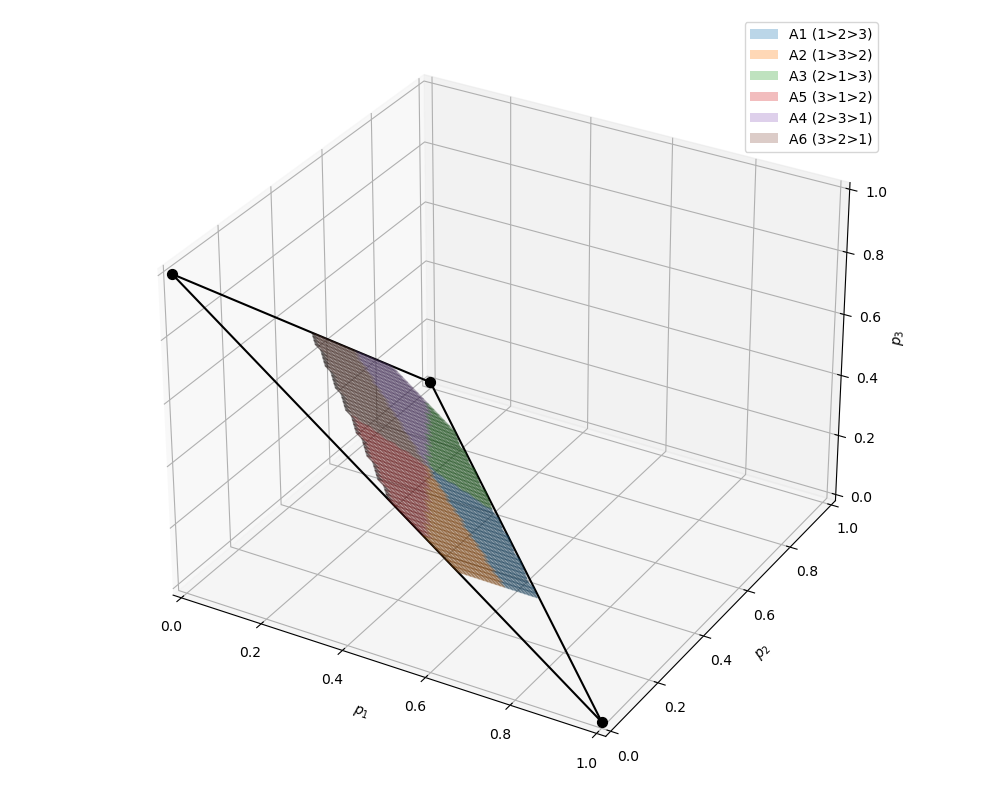
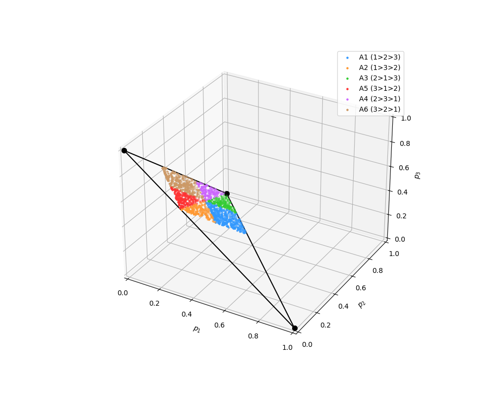
Graphical illustrations. Figure 2 illustrates two consideration structures satisfying Corollary 1, showing how the shape of the ambient probability space , and the slopes of the indifference lines depend on . In both cases, any two elements are connected in the sense of Definition 1. The figure illustrates the geometry described in Corollary 1. Namely, in each panel, the three ambient indifference lines intersect at and partition into six cone-shaped truncated regions with each such region corresponding to a unique complete strict ordering on the set of alternatives. The truncation arises from the consideration structure. The feasible probability set selects the attainable traces of these regions. Thus, we have a common linear ranking arrangement, and which ranking regions are actually populated depends on the attainable index configurations.
Lack of connectivity. Let’s briefly analyze what happens when the consideration set structure is not fully connected as for the implications are particularly transparent.
Case 1: Two elements connected, one isolated (e.g., 2 and 3 connected, 1 isolated). Then is constant, and the feasible set collapses to the line segment . Comparisons for alternatives 1 and 2 () provide no information about the split between and within this segment, and . In contrast, comparisons between 2 and 3 remain informative in : reduces to a single point , while and .
Case 2: All three elements mutually disconnected. Here is constant for each , so is a single point (dimension 0). Consequently, for every pair , .
In both cases, missing connections severely limit (or completely eliminate) the identifying power of for relative probabilities among disconnected alternatives. For general , once the partitioning of structure implied by connectivity is identified (see Proposition 2 and the subsequent discussion), the analysis reduces to studying each component separately. Within each the feasible set is effectively restricted to a lower-dimensional (namely, -dimensional) subset in , and only comparisons among alternatives inside remain informative. The analysis within each such component then proceeds exactly as in the fully connected case.
3.4.3 When partitioning of by linear hyperplanes fails (Behavioral environment level)
When for , a direct calculation shows what goes wrong. On the partial indifference locus (3.14),
with denoting the survival function of the difference between two errors conditional on (Assumption 2 ensures that this is the same for all index pairs). Since , as implied by , the additional term need not vanish and generally depends on the conditional distribution and on in a nonlinear way. Varying while preserving partial indifference (3.14), together with variation in , will generally result in that retains the full affine and topological dimension of . Moreover, as illustrated in more detail below, the overlap of and may likewise have the full affine and topological dimension of .
Thus, once the rank condition fails, the “quantile” multinomial choice model described above is generally no longer available at the Behavioral environment level uniformly over .1717 17 The partial inferential value of choice probabilities at this level still applies and is discussed in Appendix D. In particular, ranking recovery at that level may fail even though choice probabilities can continue to contain ranking information on more restricted sets.1818 18 On a restricted attainable set, a violation of the rank condition need not be exposed by the available index configurations. Such a failure, however, does not rule out ranking recovery under a more specific structural model as one can move down to the Structural environment level and fix , thus fixing function . The relevant question becomes whether the resulting model-specific mapping from indices into choice probabilities still separates the rankings.
3.4.4 A more modest perspective: the Structural environment level?
A Structural environment “quantile” property requires a common ranking partition of its probability domain , with this domain jointly attainable as varies over . Even when it exists, a particular may attain only a trace of the partition. When it fails to exist, ranking recovery within the Structural environment may still be possible for a fixed .
Even for the fixed- structural model level, ranking recovery is not automatic. The fundamental difficulty is that Assumption 2 imposes no restriction on how the joint distribution of changes with . If those changes are discontinuous in , the indifference set need not be in a -dimensional manifold, and even if it is, it may have self-intersections or other singularities that prevent separation of the ordering regions.
Stochastic independence of and . Consider with independent of . This case provides an example of being a well-behaved -manifold with desirable separability properties and then highlights how this separability may fail once independence is relaxed.
Suppose with , and suppose are distinct. Let denote the bivariate copula of , and let denote the common marginal c.d.f. of for every permutation of . In line with Assumption 2, and are absolutely continuous. For , define . Then, for example,
with analogous expressions for the other alternatives.
On , and . Write this common difference as and set , . The partial indifference locus can then be equivalently parametrized by or :
| (3.18) |
and . Since , both coordinates are strictly increasing in . Thus, under stochastic independence of and , the image of pairwise index indifference is a well defined one-dimensional curve in . Its shape, however, depends on the difference copula through and is generally nonlinear but it does not depend on a particular as it is fully indexed by .
The left panel of Figure 3 illustrates this nonlinearity for i.i.d. standard normal unobservables. It depicts the slope ratio , where is a special case of (3.18): , . For attention probabilities used in the figure, the slope ratio varies smoothly from to . Hence the partial indifference locus cannot be a straight line.
The right panel illustrates that also depends on the distribution of the unobservables, even when every candidate distribution is fully exchangeable, absolutely continuous, and independent of . Three specifications are compared. In the first, , where is uniformly distributed over the six coordinate permutations of , independently of (smooth permutation-Gaussian mixture). The second specification is the i.i.d. normal benchmark . In the third, , where , with independent of (common scale normal). The display focuses on , where the differences between curves are particularly visible.1919 19 This comparison is not intended to hold the marginal difference distribution fixed and each specification is parameterized by its own percentile . Thus, at the Structural environment level, is not determined by the attention probabilities alone but it does meaningfully separate into disjoint ordering regions: for it holds that and , placing the choice probability vector strictly above the indifference curve, while the inequalities reverse when .


Left: the slope ratio under i.i.d. standard normal unobservables.
Right: a zoomed plot of in the original coordinates for the smooth permutation-Gaussian mixture (solid), the i.i.d. normal model (dashed), and the two-scale Gaussian mixture (dotted) described in the text. The displayed range is .
Distribution of depends on . When the distribution of depends on , the findings change. Continuing with and now even fixing , the set is described as a collection of choice probabilities with
where denotes the bivariate copula of and is the c.d.f. of . Thus, the choice probabilities depend on what can be taken to be a parameter but also depend on .
First, in need not have topological dimension one less than that of . Even when it does, it need not be contained in a codimension-one embedded manifold of . This is once again because Assumption 2 imposes no restriction on how the joint distribution of varies with , allowing it potentially to vary discontinuously. Even if, in a particular structural model, is contained in a codimension-one embedded manifold, this alone does not guarantee the required separation property. The way the ordering images and are generated may itself vary discontinuously with , as illustrated below, so that probability vectors associated with opposite rankings can lie on the same side of, or overlap across, the partial indifference locus. Consequently, may fail to separate into the two disjoint ordering regions and . Imposing suitable continuity in of the distribution of would not by itself resolve the problem. Such continuity may produce a codimension-one indifference image, but it need not have separation properties as self-intersections or other singularities may remain. Thus, additional structure is required for to deliver the desired separation property.
The right panel of Figure 3 can help illustrate what can happen under such dependence. Suppose all are one-dimensional with . Let the conditional unobservable distribution be the smooth permutation-Gaussian model when , the two-scale Gaussian mixture when , and the i.i.d. normal model when . The pairwise indifference locus then jumps between the upper and lower curves in the right panel as crosses . Since these loci are distinct and bound a nondegenerate strip of the simplex over the displayed range of , the regions and overlap inside . Thus, even though each fixed conditional distribution produces a smooth indifference curve, allowing the distribution to vary discontinuously with destroys ranking recovery even for the fixed .
Even imposing an -invariant trivariate copula, including the independence one of 14, does not generally restore the separation property of . The induced bivariate copula of may still vary with through . Thus, outside the settings covered by Theorem 4, we need additional assumptions on how varies with for to yield a meaningful partition and guarantee ranking recovery.
One such assumption is a common location-scale structure for the unobservables: , where is independent of .
Fix alternative 1 as a reference and define . Let be the relative interior of the support of in its -dimensional affine hull, and let denote the attainable normalized index set restricted to . Note that and have the same sign. Theorem 5 proves a common structural partitioning at the Structural environment uniformly over and, in particular, implies the ranking recovery property.
THEOREM 5 (Common structural partition and ranking recovery).
Suppose Assumptions 3–5 hold, every two alternatives are connected in the sense of Definition 1, and , , where is independent of and has an absolutely continuous exchangeable distribution whose support is convex and has nonempty interior. Then
A. (Ranking recovery) The map under which the choice probability vector at is whenever is a topological embedding. Hence, for every , each probability vector in uniquely determines the normalized index vector and therefore all pairwise rankings of the deterministic utility indices.
B. (Common pairwise separation) for every and , . The same identity holds with replaced by or by . The second set on the right-hand side of each identity is common to all , and changes only its attained portion.
C. (Common structural partitioning) For every , , is an embedded -dimensional topological manifold in . Its complement in has exactly two connected components, and . Moreover, , and the strict order regions are all nonempty and connected, with in the closure of each.
Thus, Theorem 5 establishes that the Structural environment induces a common ranking partition of , with potentially only a trace of it attained for a given . It is more than fixed- ranking recovery as a structural ranking rule is common to all . If, in addition, , the common structural partition is fully attained as varies. The Structural environment is then “quantile” in the sense defined above.
Finally, since is a homeomorphism onto its image, the intrinsic dimension and separation properties of any attainable partition are preserved. E.g., if is an -dimensional manifold and cuts it in a separating -dimensional manifold, the corresponding probability space trace has the same dimension and separation property.
3.5 Distributional route: “quantile” version?
Let’s now maintain the standard random utility paradigm and ask when restrictions on the distribution of generate a “quantile” ranking partition or deliver only ranking recovery on the attainable probability set. Suppose generally that has a convex support with nonempty interior and an absolutely continuous distribution, with copula and marginal c.d.f.s .
Under complete index indifference (3.13), the image in the probability simplex is , . If the conditional distribution of varies freely with , then can also vary freely and need not vary continuously. Thus even total indifference need not have a single image at the Structural environment level.2020 20 It need not have a single image even at the empirical specification level, but it is not analyzed in the paper. A fixed copula and common marginals for every stabilize this point: , , does not depend on .2121 21 Unless is exchangeable, this point need not be the barycentre. Constancy of the total indifference image point is not, however, enough for ranking recovery. As the shape of changes with , the map from index differences to probabilities also changes with , so probability vectors generated by opposite index rankings may overlap. Appendix E gives an explicit overlap construction, and Proposition 3 there formalizes the resulting failure of distribution-robust ranking recovery even for a fixed .
Just like in the limited attention models in Section 3.4.4, a common location-scale structure removes this source of ambiguity by producing one fixed probability map and letting its indifference boundaries to be nonlinear. It is generally asymmetric due to copula non-exchangeability (in Section 3.4.4 asymmetry of such a map was driven by non-symmetric attention probabilities).
THEOREM 6 (Common structural partition and ranking recovery).
Suppose the standard random utility paradigm holds, and , , where is independent of with its distribution having convex support and nonempty interior. Suppose also that its marginals have the same absolutely continuous c.d.f. , and its absolutely continuous copula is generally non-exchangeable. Let , , and be defined as in Section 3.4.4 for this vector .
A.(Ranking recovery) The map such that the choice probability vector at is whenever is a topological embedding. For every , each probability vector in , thus, uniquely determines the normalized index vector and all pairwise index rankings.
If (complete indifference is feasible), then is the vector with coordinates , .
B.(Common pairwise separation) for every and , , with the analogous identities for and . The second set on the right- hand side of each identity (for each , , ) is common to all but its attainable trace may depend on .
C. (Common structural partitioning) For every , it holds that is an embedded -dimensional topological manifold in . Its complement in has exactly two connected components, and . If , the strict order regions are all nonempty and connected, and all have in their closure.
The same discussion as after Theorem 5 applies here. The common map guarantees more than fixed- recovery and gives the common structural ranking partition of , with a given possibly tracing only part of it. If, in addition, , the common structural partition is jointly attained as varies and the Structural environment is “quantile”.
Figure 4 illustrates both the structural indifference curve and its dependence on the unobservables distribution, for simplicity taking . In each case, is a mean-zero trivariate normal vector with unit variances. Let denote the pairwise correlation between and . We consider the following three cases of : (a) case 1 is the case of all positive correlations ; (b) case 2 is the case of one negative and two positive correlations ; (c) case 3 is the case of two negative and one positive . For these three cases, Figure 4 plots across , where
which fully characterize partial indifference cases with standing for . Figure 4 confirms that different correlation structures produce different curvatures. The map is common across values of only after the distribution of has been fixed. Within any one of these structural environments, a particular may still trace only a segment or another proper subset of the corresponding curve.

If the conditional distribution of varies with in a way that cannot be absorbed by a common location and scale, the challenges are analogous to those discussed in Section 3.4.4. Namely, there need not be a common index representation of choice probabilities across covariate values or a single map that applies at every covariate value. Different values of may then be associated with different structural maps, such as those generated by the three Gaussian specifications in Figure 4. Even if each map separately generates a smooth partial indifference codimension-one manifold, these manifolds may intersect or overlap when combined across covariate values, and probability vectors associated with opposite index rankings may coincide, producing ranking ambiguity.
4 Conclusion
A central insight of 14 is that choice probabilities can reveal ordinal information about deterministic utilities without any parametric model of the utility unobservables. That insight relies on a particular environment of utility maximization with conditionally i.i.d. unobservables, which can be considered the natural multinomial counterpart of the median benchmark in binary choice. This paper takes 14 as a starting point and asks how far the ordinal interpretation of choice probabilities extends once that benchmark is left behind, whether through behavioral departures from utility maximization, such as exogenous limited attention, or through asymmetries in the distribution of utility unobservables. The extension is far from automatic. With several alternatives, interactions across multiple comparison margins can lead to ranking ambiguity with no counterpart in binary choice.
References
- Random utility and limited consideration. Quantitative Economics 14 (1), pp. 71–116. External Links: Document Cited by: §1.
- Exogenous consideration and extended random utility. Journal of Econometrics 253, pp. 106166. External Links: Document Cited by: §1.
- Single-crossing random utility models. Econometrica 85 (2), pp. 661–674. Cited by: §1, footnote 6.
- Discrete choice under risk with limited consideration. CeMMAP Working Paper Technical Report CWP08/19, Centre for Microdata Methods and Practice, Institute for Fiscal Studies. External Links: Document Cited by: §1, footnote 16.
- Discrete choice under risk with limited consideration. American Economic Review 111 (6), pp. 1972–2006. External Links: Document Cited by: §1, §1.
- A random attention model. Journal of Political Economy 128 (7), pp. 2796–2836. Cited by: §1.
- Inferring cognitive heterogeneity from aggregate choices. Econometrica 88 (3), pp. 1269–1296. Cited by: §1.
- Semiparametric estimation of multinomial discrete-choice models using a subset of choices. RAND Journal of Economics 38 (4), pp. 1002–1019. External Links: Document Cited by: §1, footnote 1, footnote 2.
- Tests of symmetry for bivariate copulas. Annals of the Institute of Statistical Mathematics 64 (4), pp. 811–834. External Links: Document Cited by: Appendix C.
- Regular quantal response equilibrium. Experimental Economics 8 (4), pp. 347–367. Cited by: footnote 1, footnote 2.
- Random consideration and choice: a case study of “default” options. Mathematical Social Sciences 102, pp. 73–84. External Links: Document Cited by: footnote 13.
- Smoothed binary regression quantiles. Journal of Applied Econometrics 21 (3), pp. 387–407. Cited by: §1.
- Construction of asymmetric multivariate copulas. Journal of Multivariate Analysis 99 (10), pp. 2234–2250. External Links: Document Cited by: Appendix C, Appendix C.
- Maximum score estimation of the stochastic utility model of choice. Journal of Econometrics 3 (3), pp. 205–228. Cited by: §1, §1, §1, §2.1, §2.1, §2, Figure 1, Figure 1, §3.1, §3.1, §3.1, §3.1, §3.2, §3.2, §3.3, §3.3, §3.3, §3.3, §3.3, §3.4.4, §4, Remark 2, footnote 1, footnote 4.
- Semiparametric analysis of discrete response: asymptotic properties of the maximum score estimator. Journal of Econometrics 27 (3), pp. 313–333. Cited by: §1, §1, §2, §2, Remark 1, Remark 2.
- Identification of binary response models. Journal of the American Statistical Association 83 (403), pp. 729–738. Cited by: §1, §1, §2, §2, §2, Remark 1, Remark 2.
- Stochastic choice and consideration sets. Econometrica 82 (3), pp. 1153–1176. Cited by: §1, footnote 13.
- Revealed attention. American Economic Review 102 (5), pp. 2183–2205. Cited by: §1.
- Nonparametric identification and estimation of polychotomous choice models. Journal of Econometrics 58 (1-2), pp. 137–168. Cited by: §1.
- An introduction to copulas. 2 edition, Springer, New York. External Links: Document Cited by: Appendix C.
- Smoothed quantile regression processes for binary response models. Econometric Theory 36 (2), pp. 292–330. Cited by: §1.
Appendix
Appendix A Proofs and further examples for sections 2 and 3
Proof of Theorem 1. Exchangeability of in Assumption 1 implies that the distribution of is symmetric, with absolute continuity guaranteeing that . Convexity and nonempty interior of the joint support imply that the support of is an interval with zero in its interior. Thus its c.d.f. is strictly increasing on the interior of its support, and
| (A.1) |
A. Use the fact that condition (2) can be written as a.e. (and, of course, it implies .) Using the law of total probability and some simple algebra,
| (A.2) |
Using (A.1) and the properties of the right-hand side of (A.1) under Assumption 1, and also taking into account that by condition (1), we obtain that
C. Let us show that for every fixed , there exists a generic model satisfying Assumption 1 and the strict version of Condition (1), but violating Condition (2) on a set of positive -measure, for which ((1.2)) fails.
Fix . Let have full support on , and let and be independent standard normal random variables, independent of . Set , . Then Assumption 1 holds and . Choose sufficiently small that all the probabilities below belong to . By continuity of , choose such that . Specify
The difference between these two conditional probabilities is for every , so the strict version of Condition (1) holds. Their sum, however, equals whenever , so Condition (2) fails on that set. Since and has full support, this set has positive -measure. For every in this set, the law of total probability gives
where the inequality follows from the choice of . Hence, on a set of positive -measure,
contradicting (1.2).
Proof of Proposition 1. Relation (A.1) and condition (1) of Theorem 1 imply
Condition (2) implies then that This inequality only provides a meaningful upper bound (that is, less than 1) if . Condition (2) also implies that
This provides a meaningful lower bound (that is, greater than 0) only when .
Proof of Theorem 2.
A. By the law of total probability,
Condition (2’) gives
Hence
By the maintained support conditions, the second factor is strictly positive, zero, or strictly negative according as , , or . Condition (1’) implies that the first factor is strictly positive a.e. Therefore
which proves (1.2).
B and C. The proofs are analogous to those of parts B and C of Theorem 1. For part B, is replaced by , with the required strict inequalities following from the support conditions. For part C, the construction used there satisfies the present support conditions and Condition (2’) reduces to Condition (2).
Proof of Theorem 3. It is enough to show this for the first two options.
Take the difference for and :
There are three terms on the right-hand side of the last difference. The third term is 0 as implied by Condition (3) of the theorem (we would have to use a law of total probability in this step). As for the first and second terms, Conditions (2) and (3) imply that
Thus, the difference then can be rewritten as
Condition (1) of the theorem implies that a.e. in . Therefore,
Note that
Since all the conditional marginal distributions , , are the same and the copula is exchangeable, we can equivalently write
By copula properties, is increasing in . As implies
then using this monotonicity property we conclude that . Analogous analysis lets us conclude that for any , having implies .
Suppose now we have . Suppose, contrary to what we want to prove, we have . Then, from what we have already shown, we are guaranteed , which is a contradiction to the supposition of .
Proof of Proposition 2. Suppose some and are not connected in the sense of Definition 1. Let denote the set of all the elements in connected to in the sense of Definition 1, . By the conditions of this theorem and the construction, we have , , and , and and are disjoint connected components. Moreover, no active consideration set can intersect both and its complement: for , if and , then . In light of this,
where the last expression does not depend on .
It remains to show that is a proper subset of and that the constant lies in . By construction, and , so .
By Assumption 4, there exists an active set with , which must satisfy , implying . Likewise, there exists an active set with , where and , so and hence .
Therefore, , and is a constant in (a.e.).
Proof of Theorem 4. The exchangeability of the joint distribution of unobservables conditional on implies that for any and any permutation of ,
Denote the first function as and the second one as .
We have 3 equations: for it is
| (A.3) |
and analogous for , . These equations do not depend on the order of indices , , . The system of the three equations in the form of (A.3) has only two linearly independent equations. Thus, without a loss of generality, we can consider just the equations for and .
To characterize , we have to look at the collection of choice probabilities obtained under . With this equality enforced, let us denote . For sufficiency, no restriction on the attainable range of this value is needed. At the collection of such indices we have the following relations:
| (A.4) | ||||
| (A.5) | ||||
| (A.6) |
Equation (A.6) is a linear combination of the first two equation, therefore we can just focus on those two equations. On the right-hand sides of (A.4)-(A.5) we have only two unknowns: and . With respect to these unknowns our system is linear and has as the matrix of coefficients corresponding to . The -th row in if obtained from the equation for , , in (A.4)-(A.5).
Sufficiency. First, suppose the rank of is 1. This means that for some and with at least one of being strictly positive. Then we find that equations (A.4)-(A.5) give the relationship and, now employing equation (A.3) and analogous equation for we can conclude that if ( where denotes the interior of the support of ), then iff
If then this means that and and can be equivalently characterized by .
If , then at least one of and must be strictly positive. (i) If they are both strictly positive, this implies that and we can just take , . We then note that can be equivalently rewritten as . (ii) If one of , is 0 – e.g., , then and necessarily whereas can be any positive number. can be described by . In the other situation when and , we have and is any positive number. then is described by .
To summarize all these cases, when the rank of is 1, we have and as described in the theorem. in all the cases are intervals. so they have affine and topological dimensions 1, whereas and are 2-dimensional (from both affine and topological perspectives) sections of the plane.
Now suppose the rank of is 0. This means that , and, hence, is not connected to either or . At the same time, as the theorem states that and are connected. Note that in this case and a.e. . Thus, itself is an interval (hence, has affine and topological dimension 1). When , equations (A.4)-(A.5) give and , equivalently rewritten in this case as , . Thus, is a point (has affine and topological dimension 0). Now employing equation (A.3) and analogous equation for we can conclude that if , then iff , or, equivalently, iff , or equivalently, iff (since a.e. in this case). Thus, and are intervals and have affine and topological dimension 1.
Necessity. Let be linear in . Contrary to the statement of the proposition, suppose the rank of is 2. This implies that and . Linear has to pass through point obtained for the case of the overall indifference. Taking into account that the sum of all choice probabilities is 1, we can thus characterize this linear as the set of vectors that satisfy where at least one , When and are replaced by and , respectively, this relation has an implication with the first two-equations (A.4)-(A.5) giving us
| (A.7) |
Since a Behavioral environment separator must be valid for every admissible conditional distribution of the unobservables, it suffices to restrict attention to one admissible -invariant exchangeable distribution. We do so throughout this necessity argument.
If , then the fact that and implies that . Equation (A.7) is possible only if which gives us a contradiction for . Thus .
If , then implies that . Equation (A.7) is then possible only if which gives us a contradiction for . Thus,
Having and , we obtain that for any we can write
Under the additional index variation condition used for the converse and mentioned before the theorem in the main text, can be taken arbitrarily far in either direction. If is taken arbitrarily close to the lower support point of the distribution of , it gives us If is taken arbitrarily close to the upper support point of the distribution of , it gives us . This is clearly a contradiction.
Proof of Theorem 5. A. Under the common location-scale representation, common location terms cancel and
Thus the choice probability vector depends on only through , which defines on . Connectivity and interior support imply that every alternative is chosen with positive probability on this domain, so , and absolute continuity gives continuity.
To prove injectivity, take with , and let . If is nonempty, then and when , . Every alternative in therefore becomes strictly more attractive relative to every alternative outside . Connectivity of the consideration set structure and the nonempty interior of the unobservables support imply . If is empty, apply the same argument after reversing and . Hence is injective. Since the projection of onto the last coordinates is open in , invariance of domain implies that is a homeomorphism onto its image, and thus a topological embedding. Its inverse therefore recovers and all pairwise signs .
B. For any , injectivity gives . Taking and proves the displayed identity, and the cases and are identical. The set and its image do not depend on , whereas may. This proves statements on the common partition and attainable trace.
C. is relatively open and convex in . Moreover, exchangeability and convexity of the support imply that . Hence, for every , we have that is a nonempty relatively open subset of a -dimensional hyperplane and therefore a -dimensional topological manifold. Its complement in has exactly two connected components, and , which are nonempty and convex. Since is a homeomorphism onto its image, the same manifold and separation properties hold for their images under . Finally, relative openness at implies that every strict order region in the index space intersects arbitrarily close to . Each such intersection is convex and, hence, connected. Thus, all strict order regions in the probability space are nonempty and connected, and continuity of implies that lies in the closure of each.
Proof of Theorem 6. A. The location-scale representation again makes the choice probability vector a function of alone. Interior support implies that every alternative has positive winning probability on , and absolute continuity gives continuity. The same set argument used above proves injectivity: if is nonempty, every deterministic utility difference across the cut from to increases strictly. Convexity and nonempty interior of the unobservables support give positive probability to realizations for which the maximizer moves from to , so .
Reversing and covers the remaining case. Invariance of domain then makes a topological embedding.
At complete indifference, the common marginal c.d.f. give Whenever , the left-hand side is .
B. Analogous to the proof of Theorem 5. Injectivity of implies that, for any , it is true that . Taking and , for , we have .
C. is relatively open and convex in . For any , identical marginal distributions imply and . Hence, contains points on both sides of . By convexity, is a nonempty relatively open subset of a -dimensional hyperplane (and hence a -dimensional topological manifold). Its complement in has exactly two connected components, and , which are convex. Since is a homeomorphism onto its image, the same manifold and separation properties hold for their images under . Finally, if , relative openness implies that every strict order region intersects arbitrarily close to . Each such intersection is convex and hence connected. Thus all strict order regions in the probability space are nonempty and connected, and continuity of implies that lies in the closure of each.
Appendix B Linear ranking separators for
This appendix extends Theorem 4. Fix two distinct alternatives . The analogue of the matrix used for is
| (B.1) |
Thus, the first block records menus that contain both and and at least one other alternative, while the second block records otherwise matched menus that contain only one member of the pair.
Just like in Theorem 4, the sufficient rank condition in Theorem 7 below again applies on the attainable index set. For the converse, we additionally require sufficiently rich joint variation in the index differences.
THEOREM 7.
Suppose Assumptions 2–5 hold and . Let and be connected in the sense of Definition 1. The strict characterizations below apply to probability vectors generated at index vectors in the interior of the support of , as in the proof of Theorem 4. Then:
A. If , pairwise ranking can be recovered by a linear hyperplane involving only and on every attainable interior configuration. Under the additional index variation condition before the theorem, the converse also holds.
This rank condition is equivalent to the following restrictions: for every pair of nonempty sets ,
| (B.2) |
B. If , then coincides with the intersection of and the hyperplane
| (B.3) |
The set coincides with the intersection of and the open half-space obtained by replacing equality in (B.3) with .
C. If . Then no active menu connects either or to any outside alternative. Since and are connected, , and
The interpretation of (B.2) is similar to the case . The first equality in (B.2) requires the probabilities of matched menus containing and separately to be proportional across outside sets. The second requires them to be equal whenever an active menu contains both alternatives and at least one outside alternative.
Proof of Theorem 7. For every nonempty consideration set and , let . Then .
Let and impose . For each nonempty , exchangeability under the transposition of and gives , , and also . Consequently, the individual choice probabilities on the pairwise-indifference locus are
| (B.4) |
Considering deviations from values at total indifference, we rewrite equation in (B.4) as
| (B.5) |
A. We start by proving equivalence of the rank condition to (B.2). Write the two types of columns of as , , where . All minors formed from two common-menu columns , vanish identically. The minor formed from , is and the minor formed from , is . Thus all two-by-two minors vanish iff (B.2) holds.
Necessity. Suppose constants , not both zero, satisfy
| (B.6) |
for every probability vector generated with in the behavioral environment. By (B.5), this is for every admissible vector of menu-level deviations . Write , . Then (B.6) implies for every attainable tied index vector. Fix and . We now use the additional index variation condition imposed for the converse before the theorem. Since the index differences range over all of , for every there exists an attainable sequence of tied index configurations that, after a common normalization, satisfies , , with for and for . Since a Behavioral environment separator must be valid for every admissible conditional distribution of the unobservables, for the converse it suffices to restrict attention to one admissible -invariant exchangeable distribution. We do so throughout this necessity argument. Menus containing an element of make the probability of choosing converge to zero, whereas alternatives whose indices tend to become irrelevant. By dominated convergence, from the above we get
| (B.7) |
where does not depend on , and , Exchangeability and absolute continuity imply . Then , and . Evaluating (B.7) at these three limits gives , , and . Hence for every .
As varies, these are all cumulative subset sums of the coefficients and . Möbius inversion on the subset lattice therefore gives for every containing . Repeating the argument for each yields for every nonempty , which is precisely . A nonzero left-null vector exists only when .
Sufficiency. It is established in Parts B and C.
B. Define , . If has rank one, its two rows are proportional and therefore . Multiplying (B.5) by the left null vector gives , which is exactly (B.3).
It remains to show that the same linear functional has the strict sign of away from indifference. Let .
There are two cases. First, suppose for at least one nonempty . A positive common-menu column and rank one force the two rows of to be identical. Thus and for every . Then
| (B.8) |
Second, suppose all common-menu probabilities in the first block of are zero. Rank one implies proportionality of the two exclusive-menu rows, so for every , . A direct expansion gives
| (B.9) |
If one exclusive-menu row is zero, connectivity of and implies , so the first coefficient in (B.9) is then strictly positive.
Each difference in (B.8) and (B.9) has the weak sign of . For a common menu this follows by applying the ranking property under exchangeability to the restriction of to that menu. For matched exclusive menus, the two probabilities are evaluations of the same function: , and exchangeability makes this function the same for , and increasing in their respective indices. At index vectors in the interior of the conditional support, every active informative term is strict when . Hence, . This proves the equality and strict half-space characterizations and the separation claim. If the whole consideration set structure is connected, has affine dimension , and the zero set of has affine dimension and passes through .
C. Suppose . Then every menu containing one member of the pair and at least one outside alternative has zero probability, including every menu containing both members and an outside alternative. Since and are connected, then necessarily and , .Exchangeability and the interior-support condition imply that these centered probabilities are both zero exactly when , and have the signs stated in part C when .
COROLLARY 2.
Suppose Assumptions 2– 5 hold, , and the whole consideration set structure is connected. Let in (B.1) have rank one for every distinct pair .
Then the pairwise indifference hyperplanes in (B.3), viewed as ambient hyperplanes in , all pass through and divide into regions, one for each complete strict ordering of the utility indices. On the attainable probability set, the trace of each ambient region coincides with the corresponding strict ranking region. These traces are pairwise disjoint but need not all be nonempty.
Corollary 2 delivers a “quantile” multinomial choice model at the Behavioral environment level as the rank-one conditions for all pairs generate a global linear partition into regions, one for each complete strict ordering of the deterministic utility indices. The partition depends only on the attention probabilities and is common across all admissible conditionally exchangeable distributions of unobservables and all . As in the case, the attainable probability set inherits the corresponding traces, some of which may be empty.
The rank condition in Theorem 7 concerns hyperplanes that can be written using only and . Allowing the other choice-probability coordinates gives a strictly larger class of separators. The next result provides a direct primitive condition for such a separator. The coefficients on and are normalized to and . This is without loss of generality as adding the same constant to all coefficients does not change a linear functional on the simplex, and multiplying all coefficients by a positive constant does not change either the hyperplane or its two sides.
THEOREM 8.
Suppose Assumptions 2–5 hold and . Fix two distinct alternatives . Suppose numbers , , can be chosen so that:
- (i)
If for some , then for every .
- (ii)
For every nonempty such that ,
(B.10) - (iii)
If for some nonempty , then for every .
If and , , are connected, then
| (B.11) |
coincides, on probability vectors generated at index vectors in the interior of the conditional support, with . Replacing equality in (B.11) with gives , and replacing it with gives . If the attainable probability set has affine dimension , the indifference hyperplane has affine dimension .
The three conditions have a simple interpretation. A menu containing neither nor must receive a common coefficient, so its contribution drops out. For matched menus and , the common coefficient assigned to the alternatives in is determined by their two attention probabilities. A menu containing both alternatives forces every other alternative in that menu to receive the midpoint coefficient, which is zero under the normalization used in the theorem.
Proof of Theorem 8. Fix and denote , . The left-hand side of (B.11) once we have substituted a specific realization of the probability vector and is
| (B.12) |
Let’s evaluate the contribution to (B.12) of each type of menu.
First, let . By condition (i), all alternatives in an active such menu have a common coefficient, say . Hence its contribution , Singleton menus also contribute zero to (B.12).
Second, consider a menu with nonempty . Condition (iii) gives for every , so its contribution is . The same formula, with , applies to the menu .
Third, fix a nonempty outside set and consider the matched exclusive menus and . If , the pair contributes nothing. Otherwise, condition (ii) assigns every the common coefficient . Using , the contribution of the first menu is
Similarly, the contribution of is . Taking into account that , the combined contribution of the two matched menus is
Combining the three cases yields the explicit decomposition
| (B.13) |
Using the same approach as in the case , we can show that every difference in (B.13) has the weak sign of . At index vectors in the interior of the conditional support, each such difference is strict when .
In addition, note that all weights in (B.13) are nonnegative. Connectedness of and together with conditions (i)-(iii) guarantees that at least one of them is strictly positive.
All the facts allow us to conclude that and This proves the equality and the two strict half-space characterizations in the theorem. Finally, if the attainable probability set has affine dimension , the nonzero affine functional cuts its affine hull in a hyperplane of dimension .
The same argument gives the analogue of Corollary 1 without requiring the pairwise hyperplanes to use only the two coordinates being compared.
COROLLARY 3.
Suppose the whole consideration set structure is connected and the assumptions and conditions (i)-(iii) of Theorem 8 hold for any distinct pair , .
Then for all pairwise indifference hyperplanes their strict half-spaces identify the sign of every pairwise index difference. Namely, for any permutation of , the region associated with the index vector in the interior of the conditional distribution of and satisfying is the intersection of the strict half-spaces corresponding to the adjacent pairs . Regions associated with distinct permutations are disjoint.
Unlike Corollary 2, this result allows the hyperplane for a given pair to use different coefficients on different outside coordinates. Thus, full ordinal recovery may hold even when one or more of the two-coordinate matrices in (B.1) have rank two.
Theorem 7 is the special case of Theorem 8 in which the coefficients can be chosen equal for all . Indeed, if their common value is , then (B.11) is equivalent, using , to . Condition (B.10) then requires the same attention ratio across all outside sets, while any active menu containing both and forces . These are exactly the rank-one restrictions in Theorem 7.
Example 5 below shows that for , a partitioning hyperplane involving other probability coordinates may exist even when conditions of Theorem 7 fail.
EXAMPLE 5.
Let and suppose the only active non-singleton menus are , , , and , with all four attention probabilities positive. Set
Then has the strict sign of . A separator using only and requires , which is precisely the proportionality restriction in Theorem 7. Hence, whenever , the two-coordinate matrix has rank two but the four-coordinate hyperplane still separates the pairwise ordering.
Appendix C Non-exchangeable bivariate copulas and the quantile threshold
First, we show that any quantile index can be generated by a suitable absolutely continuous joint distribution of the unobservables . This corresponds to the special case of Theorem 2 in which the conditional marginal distributions of the two unobservables are the same, so that departures from the benchmark ordering probability are driven entirely by the copula.
Proof. We are going to use absolutely continuous checkerboard copulas. Let . First suppose with . Partition into intervals , , and set . Define This is a nonnegative density with uniform margins, hence defines an absolutely continuous copula. Since exactly of the occupied squares lie above the diagonal, For general , choose rationals . By the previous step, there are absolutely continuous copulas with , . With , , the copula is absolutely continuous and satisfies .
We next give two parametric families of absolutely continuous bivariate copulas that can generate non-exchangeability.
Liebscher–Khoudraji copulas. Let where and are absolutely continuous copulas. Then is an absolutely continuous copula. The construction is generally non-exchangeable when the two arguments are treated asymmetrically, for example when or when the two component copulas differ in a way that is not symmetric. The diagonal-ordering probability varies continuously with , see 13.
Iterated FGM copulas. A simple absolutely continuous non-exchangeable family is obtained from the asymmetric FGM-type specification
Its density is Hence is a copula, and is absolutely continuous, whenever The family is exchangeable when , but generally non-exchangeable when . Moreover,
Thus determines the direction of asymmetry, while controls its magnitude. This gives a transparent calibration device for , subject to the admissible range of .
Appendix D What survives when the rank condition fails (Behavioral environment level)
For simplicity, consider . Let be a permutation of . When , we necessarily have and . Theorem 4 then rules out a common linear partition at the Behavioral environment level. Here we show what can still be learned in this case.
Suppose Assumptions 2–5 hold and . Then, for every ,
In particular, if , then
Consequently,
Thus, outside of the strip
the sign of is recovered uniformly over the Behavioral environment. Inside the strip, we cannot make a ranking claim at the Behavioral environment level (even though a particular Structural environment may still be informative there). As attention neutrality is approached, , the strip collapses to the hyperplane that appears in the rank-one case of Theorem 4 when .
Looking at this from the econometrics perspective, one can conclude that still contains valuable information about the underlying indices and parameter . However, as is typical in these models, the most valuable cases are when underlying indices are extremely close to indifference which will be ruled out by the strip.
Appendix E Distributional route: Additional details for Section 3.5
This appendix records additional details behind the discussion in Section 3.5.
First, let’s make it explicit why a fixed copula and common conditional marginals stabilize the image of total indifference but do not, by themselves, produce a common partial-indifference boundary.
Consider the image in of an that corresponds to the case of complete indifference (3.13):
We already see a difference with the behavioral route of consideration sets. Here, even at the level of an empirical specification (that is, for fixed ), collecting such images across may trace out a set whose affine and topological dimension from zero (when this point does not depend on ) to (when the convex hull of such points has a relative interior in ). Passing from the empirical specification to the corresponding fixed- structural model enlarges the covariate domain from to . Hence the resulting collection of image points can only expand, so its affine and topological dimensions can increase (up to ) or remain unchanged. An analogous weak expansion conclusion applies when passing from a fixed- structural model to the corresponding fixed- behavioral specification , since the latter ranges over the admissible conditional distributions in . At the heart of the broadness of such conclusions is, once again, the fact that the properties of the behavior of the joint distribution of unobservables conditional on with respect to are unrestricted (e.g., does not necessarily even change continuously). To have a hope of getting an analogue of a “quantile model” at the Structural environment level, it is at least necessary to ensure that does not vary with .
Suppose that (i) the copula does not depend on and (ii) all unobservable have exactly the same marginal distributions: for all for any , . Then does not depend on as
does not depend on . Under conditions (i) and (ii), the notation of this image point by emphasizes that it is specific to the Structural environment. Since need not be exchangeable, we should not expect for all . Moreover, the point need not be common across the Structural environments admitted by a given Behavioral environment. Variation in the total indifference image alone, however, does not establish ranking ambiguity.
Constancy of is not sufficient for a common partial indifference boundary. To see this more explicitly, continue with restrictions (i) and (ii) above (constancy of the copula and the same conditional marginal c.d.f.) and take and , and write . Define
On the interior of the relevant difference support, both functions are strictly increasing. The partial indifference image can therefore be written as
| (E.1) |
Although the total indifference point is common, the functions , may change with through the shape of . Equation in (E.1) does not necessarily describe one curve. This identifies the additional restriction needed beyond a fixed copula and common conditional marginals: the map from normalized index differences to probabilities must itself be common across covariate values.
Suppose, in addition, that is independent of . The functions above no longer depend on and the indifference locus is the curve
where ranges over the interior of the relevant difference support. The separation property can be seen directly. Suppose , and write . Relative to the partial indifference configuration , alternative 1 becomes strictly more attractive relative to alternative 2, while alternative 2 becomes strictly less attractive relative to both alternatives 1 and 3. Monotonicity of the copula partial derivatives in the remaining arguments gives , . Since and are strictly increasing, this implies that The inequalities reverse when . Thus at the Structural environment level the partial indifference representation is a (nonlinear) curve separating the two strict ranking regions. Partial exchangeability can make one of these boundaries linear even when the full unobservables distribution is not exchangeable. If is invariant to interchanging and , then along and , The other two pairwise boundaries may remain nonlinear if alternative 3 is not exchangeable with alternatives 1 and 2. Hence linearity of one pairwise comparison does not imply an exchangeable multinomial model or a fully linear partition.
Dependence on . The curves in Figure 4 also give a direct construction of the overlap described in the main text. Let each be one-dimensional and set . Use Case 1 distribution when , Case 3 when , and Case 2 when . Each fixed distribution generates a smooth separating curve. The strip between Case 1 and Case 3 curves is on the side of Case 1 curve and on the side of Case 3 curve. Probability vectors in that strip can therefore be generated under opposite index rankings. This construction gives an explicit instance of ranking ambiguity. The following proposition records the more general point that once the admissible distributional class is sufficiently rich, failure of symmetry at pairwise index indifference can itself generate such ambiguity, even for a fixed .
Proposition 3 (Failure of distribution-robust ranking recovery).
Fix and suppose the joint index differences range over . Suppose the Behavioral environment admits an -independent, absolutely continuous distribution with common marginals and full support on , as well as the distribution obtained from it by relabeling alternatives and . If, at some index configuration satisfying (3.14), the first distribution generates , then Hence, fixed- ranking recovery fails at the Behavioral environment level.
Proof of Proposition 3. Without loss of generality, suppose that at the stated pairwise-indifferent configuration . Holding the other indices fixed, increase . The difference is continuous, starts negative, and converges to . Hence, at some configuration with , we have . Relabeling and in both the unobservables distribution and the index configuration leaves this probability vector unchanged but reverses the deterministic ranking. Full joint index difference variation makes both configurations attainable for the same .
It remains only to note that the common probability vector is in the relative interior. Under the fixed full support distribution, the map from normalized index differences to choice probabilities is continuous and injective, that is, if two index vectors differ, the choice probability of the set of alternatives whose relative indices increase changes strictly. By invariance of domain, its image is open in . Hence the constructed probability vector lies in .