OceanLight: Efficient Global Ocean Forecasting via Geometry-Adaptive Unstructured Mesh Representation

We compare our model with GLONET and graphcast, using oceanbench (2) as inputs and make predictions across different lead times. We calculate RMSE and ACC to evaluate basic forecast accuracy across variables and lead times. The result of RMSE and ACC of different variables is shown in figure 2.

Overall, our model achieves consistently lower RMSE and higher ACC than GLONET across all variables and lead times, while showing performance comparable to or slightly better than GraphCast in most cases. For sea surface height (SSH), our model obtains the lowest RMSE at nearly all forecast horizons and maintains competitive ACC values, especially at short- and medium-range lead times. In temperature prediction, our method significantly reduces RMSE compared with GLONET and GLO12 and achieves similar ACC performance to GraphCast, indicating better stability during long-term forecasting. For salinity, both RMSE and ACC results demonstrate that our model substantially outperforms GLONET, GLO12 and closely matches GraphCast, particularly at 1–7 day lead times. In the prediction of zonal and meridional currents, our model consistently achieves lower RMSE and higher ACC than GLONET and GLO12, while remaining competitive with GraphCast. Although the forecasting accuracy of all models gradually decreases as the lead time increases, our method shows a slower degradation trend, especially for dynamic variables such as ocean currents. These results demonstrate that the proposed model has strong forecasting capability and generalization performance on multiple ocean variables under the IV-TT evaluation framework.

We also conducted a depth-stratified evaluation of temperature and salinity using the IVTT metric and plotted their vertical profiles. The vertical profiles of temperature and salinity are shown in supplementary Figure S1. We have also implemented the IVTT evaluation of ocean temperature, salinity, current velocity, and sea surface height, broken down by season and region. The experimental results are presented in the figures in supplementary Figure S2-S3.

The geostrophic surface currents were diagnosed from the model-predicted sea surface height above geoid (SSH) via the geostrophic balance equations and compared with the model-predicted surface currents. Dynamical consistency between the two was quantified using the RMSE and correlation coefficient; lower RMSE and higher correlation coefficients indicate better geostrophic consistency. The geostrophic surface currents ($u_{g}$ and $v_{g}$) were derived from the model-predicted sea surface height above geoid; the calculation details are given in the supplementary note 1.

The comparison results are presented in figure 3.

The experimental results show that the our model achieves the lowest RMSE between the geostrophic currents and the predicted surface currents, indicating that the predicted dynamical height field is more physically reasonable. Since geostrophic currents are directly determined by the spatial gradients of sea surface height, the lower RMSE suggests that the proposed method produces more accurate SSH gradient structures and reconstructs more realistic ocean dynamical patterns, rather than merely reducing point-wise prediction errors.

In addition, our model achieves the highest correlation coefficients for both the zonal and meridional velocity components, demonstrating stronger consistency in the flow direction between the derived geostrophic currents and the predicted surface currents. In particular, the improvement in the meridional component ($v$) is especially significant, indicating that the model more effectively captures the two-dimensional spatial structure of SSH gradients and mesoscale ocean dynamical features.

These results demonstrate that the proposed model not only fits sea surface height fields more accurately, but also better preserves the underlying ocean dynamical consistency and geostrophic balance relationships.

To further evaluate the dynamical characteristics of the predicted ocean surface circulation, the total kinetic energy (KE), mean kinetic energy (MKE), and eddy kinetic energy (EKE) were calculated based on the predicted velocity components ($u,v$) of 0.49m, and the calculation formulas are provided in the supplementary note 5.

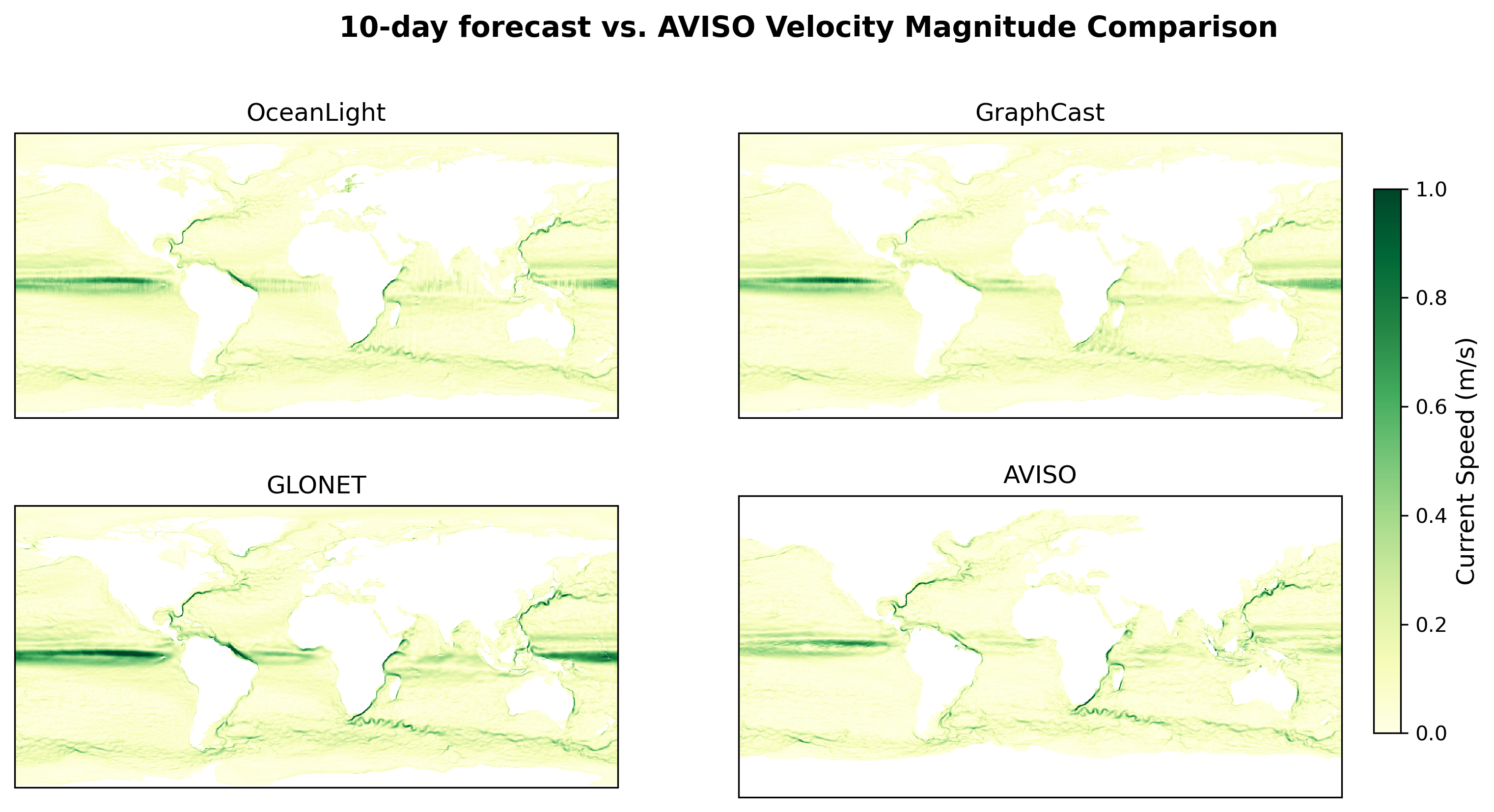
We use the AVISO dataset as the observational reference to calculate KE, MKE and EKE. The same quantities are also computed from the model-predicted surface velocity fields. To quantitatively evaluate the consistency between the model-derived and AVISO-derived energy fields, several statistical metrics are calculated, including the RMSE, variance ratio, amplitude ratio, and area integral ratio, with the computational formulas presented in the supplementary note 3. We demonstrate the KE results and its visualization in figure 4. The results of EKE, MKE are demonstrated in supplementary S14-S15.

For RMSE, our model achieves the lowest errors across KE, MKE, and EKE, demonstrating substantially improved prediction accuracy compared with both GLONET and GraphCast. For the ratio-based metrics, including variance ratio, amplitude ratio, and area integral ratio, values closer to 1 indicate better agreement with the reference data. Variance ratio represents the magnitude of spatial variation in an energy field, a value smaller than 1 indicates overly smooth predictions, while a value larger than 1 suggests exaggerated spatial fluctuations. The amplitude ratio reflects whether the average energies of the two fields are matched, and the area integral ratio indicates whether the total energies of the two fields are consistent. The results show that our model achieves most of the ratio-based metrics closer to 1, indicating better agreement with the reference fields. In contrast, GLONET exhibits substantial overestimation of energy intensity and spatial variability, as all ratio-based metrics are significantly larger than 1. This suggests that GLONET tends to excessively amplify the geostrophic energy fields and produces overly exaggerated spatial fluctuations.

To evaluate the mesoscale eddy forecasting performance, the predicted Sea Surface Height above Geoid (SSH) was first converted into Sea Level Anomaly (SLA) by subtracting the Mean Dynamic Topography (MDT). Mesoscale eddies were then identified from the resulting SLA fields using the Py-Eddy-Tracker (PET) algorithm. As the reference, mesoscale eddies were extracted from the AVISO satellite-observed SLA using the same PET algorithm, ensuring a consistent eddy identification procedure for both forecasts and observations. For eddy-based verification, a forecasted eddy was matched to an observed eddy when either of the following criteria was satisfied: the core position of the forecasted eddy fell within the effective closed contour of the observed eddy, or the distance between the forecasted eddy core and the observed eddy core was less than or equal to the effective radius of the observed eddy. Based on the matched forecasted and observed eddies, four commonly used dichotomous verification metrics, namely Probability of Detection (POD), False Alarm Ratio (FAR), Bias, and Critical Success Index (CSI) 37, were calculated to comprehensively evaluate the detection capability, reliability, systematic prediction tendency, and overall forecasting skill of our model and the baseline methods. The calculation formulas are provided in supplementary note 4. Since the AVISO altimetry product used as the observational reference for eddy detection has a spatial resolution of 0.25°, the mesoscale eddy detection comparison is restricted to baselines at matching resolution, namely GLONET and GraphCast. GLO12 is excluded from this comparison due to its higher resolution of 1/12°, as GLO12 resolves finer-scale eddies that fall below what AVISO can detect, making direct comparison against the 0.25° reference inherently unfair to its true eddy-resolving skill.The results are shown in figure 5.

Western boundary current regions are among the most dynamically active areas of the global ocean. The Kuroshio Extension, Gulf Stream, and Brazil Current are characterized by strong currents, sharp sea surface height gradients, intense baroclinic instability, and vigorous air–sea interactions. These processes favor the frequent generation, propagation, and deformation of mesoscale eddies, making such regions rich in eddy activity but also particularly challenging for ocean forecasting. Therefore, in addition to global quantitative evaluation, we further conduct regional visualization and IVTT-based assessment 38 over these three representative western boundary current regions to examine whether the model can accurately capture mesoscale eddy structures and SLA evolution in highly energetic oceanic regimes.

Thus, mesoscale eddy visualizations were conducted in three major western boundary current regions, including the Kuroshio and its extension region, the Gulf Stream, and the Brazil Current. The initial condition was taken from the OceanBench dataset on 2 January 2024, and a 10-day lead-time forecast was performed. The AVISO observational data on 12 January 2024 were used as the reference state. Mesoscale eddies were identified from both the forecasted and observed SLA fields using the PET algorithm 32, and the corresponding detection results are shown in supplementary Figure S4-S6.

To ensure a fair comparison with GraphCast, our unstructured mesh-based graph neural network model adopts identical hyperparameter settings, i.e., an embedding size of 512 and blocks number of 16.

As shown in table 1, compared with GraphCast, our model reduces the numbers of mesh nodes and mesh edges by approximately 97.0% and 99.9%, respectively, and decreases the grid→mesh edges and mesh→grid edges by approximately 55.7% and 76.8%, respectively. The significant reduction in the number of edges and nodes greatly decreases both the FLOPs and the memory usage during model operation, as shown in table 2. Specifically, FLOPs are reduced by 73.0%, while Max Memory Reserved and Max Memory Allocated are reduced by 62.4% and 62.3%, respectively. The decrease in FLOPs also greatly reduces the time cost of model training, and the time decomposition of model training is illustrated in the figure 6.

Compared to GraphCast, our model reduces the training time of the encoder, processor, decoder, and backpropagation by 40.3%, 92.2%, 61.4%, and 71.2%, respectively.

The core architecture follows the established encode-process-decode paradigm used in GraphCast. Given an input ocean state at time $t$, the model predicts the ocean state at time $t+\Delta t$. The key distinction lies in the graph topology: instead of uniform refinement to an icosahedral mesh, our model operates on unstructured mesh comprising 1,212 regions based on ocean climatology data. This results in a substantially sparser graph structure, with only 4,120 edges connecting mesh nodes, and 681,067 bidirectional edges linking grid and mesh nodes. Compared to GraphCast’s dense mesh, our unstructured representation reduces the number of mesh nodes and edges by over an order of magnitude, cutting GPU memory usage by over 50% while preserving—and even slightly improving—the model’s capacity to resolve regionally varying ocean dynamics. Based on the graph structure constructed from the above process, we use $\mathbf{v}_{\scriptscriptstyle G}$, $\mathbf{v}_{\scriptscriptstyle M}$, $\mathbf{e}_{\scriptscriptstyle G2M}$, $\mathbf{e}_{\scriptscriptstyle M2G}$, and $\mathbf{e}_{\scriptscriptstyle M2M}$ to denote the features of grid nodes, mesh nodes, edges from grid to mesh, edges from mesh to grid, and edges from mesh to mesh, respectively.

The encoder embeds grid nodes, mesh nodes, and grid-to-mesh edge features into a latent space using separate MLPs. Then it performs a gnn-based message-passing step from grid nodes to mesh nodes. In this step, the 0.25° ocean data is encoded into the unstructured mesh representation:

$$\tilde{\mathbf{v}}_{G}=\mathrm{MLP}(\mathbf{v}_{G}),\quad\tilde{\mathbf{v}}_{M}=\mathrm{MLP}(\mathbf{v}_{M}),\quad\tilde{\mathbf{e}}_{G2M}=\mathrm{MLP}(\mathbf{e}_{G2M})$$

$$\mathbf{v}_{M}^{\prime}=\tilde{\mathbf{v}}_{M}+\mathrm{InteractionNetwork}\left(\tilde{\mathbf{v}}_{G},\ \tilde{\mathbf{v}}_{M},\ \tilde{\mathbf{e}}_{G2M}\right)$$

$$\mathbf{v}_{G}^{\prime}=\tilde{\mathbf{v}}_{G}+\mathrm{MLP}(\tilde{\mathbf{v}}_{G})$$

The processor consists of 16 unshared message-passing layers that operate on the mesh representation. Each layer updates edges and nodes sequentially, followed by residual connections for both nodes and edges. For layer $l=1,\dots,L$ (unshared parameters), where $l$ denotes the index of the current processor layer among the $L$ stacked message-passing layers:

$$\mathbf{e}_{M2M}^{(l)},\ \mathbf{v}_{M}^{(l)}=\mathrm{EdgeUpdate\&NodeUpdate}\left(\mathbf{v}_{M}^{(l-1)},\ \mathbf{e}_{M2M}^{(l-1)}\right)$$

$$\mathbf{v}_{M}^{(l)}\leftarrow\left(\mathbf{v}_{M}^{(l-1)}+\mathbf{v}_{M}^{(l)}\right),\quad\mathbf{e}_{M2M}^{(l)}\leftarrow\mathbf{e}_{M2M}^{(l-1)}+\mathbf{e}_{M2M}^{(l)}$$

$$\mathbf{v}_{M}^{\mathrm{out}}=\mathbf{v}_{M}^{(L)}$$

The decoder uses MLPs to embed mesh-to-grid edge features and performs gnn-based message-passing step from mesh nodes back to grid nodes. MLPs are used for the message passing flow, converting the information contained in the meshes to grids and output the prediction:

$$\tilde{\mathbf{e}}_{M2G}=\mathrm{MLP}(\mathbf{e}_{M2G})$$

$$\mathbf{v}_{G}^{\prime\prime}=\mathbf{v}_{G}^{\prime}+\mathrm{InteractionNetwork}\left(\mathbf{v}_{M}^{\mathrm{out}},\ \mathbf{v}_{G}^{\prime},\ \tilde{\mathbf{e}}_{M2G}\right)$$

$$\hat{\mathbf{v}}_{G}^{\mathrm{out}}=\mathrm{MLP}(\mathbf{v}_{G}^{\prime\prime})$$

We obtained monthly ocean climatological data from the Copernicus Marine Environment Monitoring Service (CMEMS). For each grid point, we extract a multi-dimensional feature vector comprising various oceanographic variables, including temperature, salinity, zonal and meridional ocean current velocity components at 23 discrete depth levels (i.e., 0.49m, 2.65m, 5.08m, 7.93m, 11.41m, 15.81m, 21.60m, 29.44m, 40.34m, 55.76m, 77.85m, 92.32m, 109.73m, 130.67m, 155.85m, 186.13m, 222.48m, 266.04m, 318.13m, 380.21m, 453.94m, 541.09m and 643.57m) and sea surface height. By averaging the climatological fields of all twelve months, we construct the annual mean ocean climatology. This dataset represents the long-term mean state of the ocean and reflects its stable background characteristics. The annual mean climatological dataset provides a robust representation of the ocean’s integrated mean state on long time scales, serving as the foundational dataset for subsequent calculation and ocean graph construction.

Global ocean data at high resolution contains fine-scale details that can introduce challenges for constructing a tractable and representative adaptive mesh. The high-resolution data may contain noise, and in regions such as land-sea boundaries or strong oceanic fronts, fine-scale spatial gradients can be excessively sharp, potentially leading to an overly fragmented adaptive mesh with an impractically large number of regions. To address these issues, we employ a hierarchical multi-resolution strategy that balances computational efficiency, noise reduction, and the preservation of meaningful spatial structure for mesh construction. We regridded the data from its original resolution to a 1.40625° × 1.40625° latitude-longitude grid using the Climate Data Operators (CDO) 40 with bilinear interpolation (remapbil operator).

Denote the horizontal grids of 1.40625° ocean climatology as

$$\Omega_{c}=\{(i,j)\mid i=1,\ldots,N_{lat}^{c},\ j=1,\ldots,N_{lon}^{c}\}$$

At each grid point $(i,j)\in\Omega_{c}$, the multivariate climatological state is represented by a feature vector $\mathbf{x}_{i,j}\in\mathbb{R}^{d}$ which includes temperature, salinity, zonal and meridional velocities across multiple depth levels, as well as sea surface height. To extract dominant mode of variability, principal component analysis (PCA) 33; 22 is applied to the multivariate feature vectors, reducing it to a one-dimensional principal component. Formally, the reduced scalar value at each grid point is given by

$$z_{i,j}=\mathcal{P}(\mathbf{x}_{i,j}),\;z_{i,j}\in\mathbb{R}$$

where $\mathcal{P}(\cdot)$ denotes projection onto the first principal component via PCA. The resulting scalar field is

$$Z=\{z_{i,j}\}\in\mathbb{R}^{N_{lat}^{c}\times N_{lon}^{c}}$$

Then the spatial gradient of $Z$ is computed using the sobel operator 41. Let $\mathbf{K}_{x}$ and $\mathbf{K}_{y}$ denote the standard Sobel kernels in the zonal and meridional directions respectively, which are defined as:

$$\mathbf{K}_{x}=\begin{bmatrix}-1&0&1\\ -2&0&2\\ -1&0&1\end{bmatrix}\qquad\mathbf{K}_{y}=\begin{bmatrix}-1&-2&-1\\ 0&0&0\\ 1&2&1\end{bmatrix}$$

The discrete gradients at each grid point $(i,j)$ are calculated as:

$$G_{x}(i,j)=(\mathbf{K}_{x}*Z)(i,j)=\sum_{p=-1}^{1}\sum_{q=-1}^{1}K_{x}(p,q)Z(i+p,j+q)$$

$$G_{y}(i,j)=(\mathbf{K}_{y}*Z)(i,j)=\sum_{p=-1}^{1}\sum_{q=-1}^{1}K_{y}(p,q)Z(i+p,j+q)$$

The gradient magnitude is then given by

$$G(i,j)=\sqrt{G_{x}(i,j)^{2}+G_{y}(i,j)^{2}},$$

This resulting in the gradient map $G\in\mathbb{R}^{N_{lat}^{c}\times N_{lon}^{c}}$, and the gradient field is used exclusively to guide the selection of seed points in the subsequent region-growing procedure.

Inspired by work of adaptive multi-granularity graph representation 13, we first adopt the region growing method for initial region delineation. For any pair of adjacent grid points $(i,j)$ and $(m,n)$, the feature-space difference is defined as

$$D((i,j),(m,n))=\|\mathbf{x}_{i,j}-\mathbf{x}_{m,n}\|_{2}$$

Let $\mathcal{N}(i,j)$ denote the 8-connected neighborhood of $(i,j)$, $\tau$ denote the threshold as the domain is partitioned into spatially connected regions using the threshold-based region-growing algorithm. Let $\Omega\subseteq\Omega_{u}$ denote the set of unlabeled grid points. At each iteration, a new region is initialized from the point with the minimum gradient magnitude:

$$(i_{k},j_{k})=\arg\min_{(i,j)\in\Omega_{u}}G(i,j).$$

Starting from this seed, the region $R_{k}$ is expanded by recursively including neighboring points that satisfy the similarity criterion:

$$D((i,j),(m,n))\leq\tau,\quad(m,n)\in\mathcal{N}(i_{k},j_{k}).$$

The expansion is implemented using depth-first traversal until no further points can be added. This process is repeated until all grid points are assigned, yielding a partition

$$\Omega_{c}=\bigcup_{k=1}^{K}R_{k},\qquad R_{k}\cap R_{\ell}=\varnothing\ (k\neq\ell).$$

While the region growing algorithm preliminary partitioning method effectively handles regions such as land-sea boundaries and areas with steep gradients, it still generates large mesh regions that exceed over 20% of the total ocean grid points. Such large regions are problematic because they aggregate diverse oceanic features into a single mesh node, reducing the model’s ability to resolve spatial heterogeneity and potentially degrading forecast skill.

To further resolve large-scale structures, regions occupying more than 20% of the domain are refined using HDBSCAN clustering. For each region $R_{k}$, define its area fraction:

$$\alpha_{k}=\frac{|R_{k}|}{|\Omega_{c}|}.$$

Regions satisfying $\alpha_{k}>0.20$ are selected for refinement. For each such region, feature vectors $\mathbf{x}_{i,j}$ in the region $R_{k}$ forms a sample set

$$X_{k}=\{\mathbf{x}_{i,j}\mid(i,j)\in R_{k}\}$$

HDBSCAN partitions $X_{k}$ into clusters, inducing a decomposition $R_{k}=\bigcup_{l=1}^{L}R_{k,l}$, where each $R_{k,l}$ denotes a refined subregion. Since HDBSCAN operates in feature space, a given cluster $R_{k,l}$ may consist of multiple geographically disconnected components. To ensure spatial consistency, each cluster is further decomposed into spatially connected subregions based on grid adjacency. Specifically, for each $R_{k,l}$, we define its connected components as

$$R_{k,l}\;\longrightarrow\;\{R_{k,l}^{(1)},R_{k,l}^{(2)},\dots\},$$

where each $R_{k,l}^{(\ell)}$ is a maximal connected subset under the neighborhood relation $\mathcal{N}(i,j)$. These connected components are treated as independent regions in the final segmentation, and subclusters replace the original region, yielding a refined segmentation of the global ocean.

Following the segmentation, each region $R_{k}$ is treated as a mesh node. The set of mesh nodes is defined as

$$\mathcal{V}_{M}=\{R_{1},R_{2},\dots,R_{k}\}$$

Each mesh node $R_{k}$ is associated with a representative location in the spatial domain, defined as the centroid of the region:

$$(\bar{i}_{k},\bar{j}_{k})=\frac{1}{|R_{k}|}\sum_{(i,j)\in R_{k}}(i,j).$$

Two meshes $R_{k}$ and $R_{\ell}$ are connected if they share at least one pair of neighboring grid points:

$$(R_{k},R_{\ell})\in\mathcal{E}_{1}\iff\exists(i,j)\in R_{k},(m,n)\in R_{\ell}\text{ s.t. }(m,n)\in\mathcal{N}(i,j).$$

Here, $\mathcal{E}_{1}$ denotes the set of first-order geographical adjacency edges. To capture higher-order spatial relationships, edges are further extended based on multi-step connectivity. Let

$$\mathcal{G}_{1}=(\mathcal{V}_{M},\mathcal{E}_{1})$$

denote the first-order adjacency graph. For a given integer $k\geq 1$, define

$$\mathcal{E}_{M}=\{(R_{i},R_{j})\mid\text{dist}_{\mathcal{G}_{1}}(R_{i},R_{j})\leq k,\;R_{i}\neq R_{j}\},$$

where $\text{dist}_{\mathcal{G}_{1}}$ is the shortest-path distance. In this study, we set $k=2$. The final mesh graph is defined as

$$\mathcal{G}_{M}=(\mathcal{V}_{M},\mathcal{E}_{M})$$

where $\mathcal{E}_{M}$ includes both first-order and higher-order (k-hop) spatial connectivity.

Let

$$\Omega_{f}=\{(u,v)\mid u=1,\dots,N_{lat}^{f},v=1,\dots,N_{lon}^{f}\}$$

denote the fine-resolution spatial grid at 0.25°, on which the subsequent gnn forecasting model is applied. The set of fine-grid nodes is defined as

$$\mathcal{V}_{G}=\Omega_{f}$$

Since the mesh partition is obtained on the coarse grid, each 0.25°grid point is assigned to a mesh region based on its spatial location. Specifically, a 0.25°grid node $(u,v)$ is associated with region $R_{k}$ if its geographical coordinates fall within the spatial extent of $R_{k}$. Let

$$\phi:\Omega_{f}\rightarrow\mathcal{V}_{M}$$

denote this assignment, where $\phi(u,v)=R_{k}$ if the grid point $(u,v)$ lies within the spatial domain covered by region $R_{k}$. The grid–mesh edge set is then defined as

$$\mathcal{E}_{GM}=\{((u,v),R_{k}),(R_{k},(u,v))\mid\phi(u,v)=R_{k}\}.$$

Thus, for each 0.25°grid node $(u,v)$, two directed edges are constructed:

$$(u,v)\rightarrow R_{k},\qquad R_{k}\rightarrow(u,v),\qquad\text{if }\phi(u,v)=R_{k}$$

thereby enabling bidirectional information exchange between grid nodes and mesh nodes.

The complete graph is defined as

$$\mathcal{G}=(\mathcal{V},\mathcal{E}),$$

where

$$\mathcal{V}=\mathcal{V}_{G}\cup\mathcal{V}_{M},\quad\mathcal{E}=\mathcal{E}_{M}\cup\mathcal{E}_{GM}$$

Given the constructed edge set $\mathcal{E}_{GM}$, information is then propagated between nodes via an Interaction Network. For an arbitrary directed edge $(s,r)\in\mathcal{E}$, where $s\in\mathcal{V}$ denotes the sender node and $r\in\mathcal{V}$ the receiver node, let $x_{s}$ and $x_{r}$ denote the corresponding node features and $e_{sr}$ the edge feature. In the Interaction Network, the receiver node representation is updated through message passing, followed by aggregation and node update.

As for the message passing step, for each edge $(s,r)\in\mathcal{E}$, a message is computed by concatenating the sender feature, the receiver feature, and the edge feature, followed by a multi-layer perceptron:

$$e^{\prime}_{sr}=\mathrm{MLP}\left(\left[x_{s}\,\|\,x_{r}\,\|\,e_{sr}\right]\right),$$

where $[\cdot\|\cdot\|\cdot]$ denotes feature concatenation.

As for the aggregation and node update step, for each receiver node $r$, the messages from all its incoming edges are aggregated by summation, and the receiver representation is updated via a second multi-layer perceptron:

$$x^{\prime}_{r}=\mathrm{MLP}\left(\left[x_{r}\,\|\sum_{s\,:\,(s,r)\in\mathcal{E}}e^{\prime}_{sr}\right]\right).$$

This topological design of grid-mesh edges reduces the number of edges while preserving the essential edges for physical information transmission. Thus, the enhancement in computational efficiency is achieved without compromising forecasting performance.

The geostrophic surface currents ($u_{g}$ and $v_{g}$) were derived from the model-predicted sea surface height above geoid (SSH, denoted here as $\eta$) based on the geostrophic balance equations:

$$u_{g}=-\frac{g}{f}\frac{\partial\eta}{\partial y}$$

$$v_{g}=\frac{g}{f}\frac{\partial\eta}{\partial x}$$

where $g$ is the gravitational acceleration, $f$ is the Coriolis parameter, and $\partial\eta/\partial x$ and $\partial\eta/\partial y$ are the zonal and meridional gradients of SSH.

The geostrophic and model-predicted current speeds were calculated as

$$S_{g}=\sqrt{u_{g}^{2}+v_{g}^{2}}$$

$$S_{m}=\sqrt{u^{2}+v^{2}}$$

RMSE (Root Mean Square Error)
We use RMSE to measure pointwise prediction accuracy. It is formulated as the following:

$$\mathrm{RMSE}=\sqrt{\frac{1}{N}\sum_{i=1}^{N}(\hat{y}_{i}-y_{i})^{2}}$$

where $N$ denotes the number of grids, $\hat{y}_{i}$, denotes the predicted value, and $y_{i}$ denotes the real value.

ACC(Anomaly Correlation Coefficient)
We use ACC to assess the spatial pattern correlation with respect to climatological anomalies. It is formulated as the following:

$$ACC=\frac{\sum_{i=1}^{N}(\hat{y}_{i}-c_{i})(y_{i}-c_{i})}{\sqrt{\sum_{i=1}^{N}(\hat{y}_{i}-c_{i})^{2}}\sqrt{\sum_{i=1}^{N}(y_{i}-c_{i})^{2}}}$$

where $N$ denotes the number of grids, $\hat{y}_{i}$, denotes the predicted value, and $y_{i}$ denotes the real value, and $c_{i}$ denotes the corresponding climatology value.

Corr(Correlation Coefficient)
We use the Pearson correlation coefficient (Corr) to evaluate the consistency between the geostrophic currents derived from sea surface height and the predicted surface currents. The correlation coefficients are calculated separately for the zonal and meridional velocity components. It is formulated as follows:

$$\mathrm{Corr}=\frac{\sum_{i=1}^{N}(\hat{u}_{i}-\overline{\hat{u}})(u_{i}-\overline{u})}{\sqrt{\sum_{i=1}^{N}(\hat{u}_{i}-\overline{\hat{u}})^{2}}\sqrt{\sum_{i=1}^{N}(u_{i}-\overline{u})^{2}}}$$

where $N$ denotes the number of grids, $\hat{u}_{i}$ denotes the geostrophic current component derived from sea surface height, $u_{i}$ denotes the corresponding predicted surface current component, and $\overline{\hat{u}}$ and $\overline{u}$ denote their spatial mean values, respectively. The same formulation is applied to the meridional velocity component.

To quantitatively evaluate the consistency between the model-predicted and observation-derived ocean surface kinetic energy fields, three spatial ratio metrics are applied to each energy variable — total kinetic energy (KE), mean kinetic energy (MKE), and eddy kinetic energy (EKE). These metrics assess different aspects of energy agreement: the spatial variability amplitude, the mean energy intensity, and the total integrated energy magnitude, respectively. For a given energy field $X\in\{\mathrm{KE},\,\mathrm{MKE},\,\mathrm{EKE}\}$, the three metrics are defined as follows.
Variance ratio
We use the variance ratio to evaluate whether the spatial variability amplitude of the model-predicted field is realistically reproduced. It is formulated as follows:

$$\mathrm{Variance\ Ratio}(X)=\frac{\mathrm{Var}(X_{\mathrm{model}})}{\mathrm{Var}(X_{\mathrm{obs}})}=\frac{\displaystyle\sum_{i=1}^{N}\sum_{j=1}^{M}\bigl(X_{\mathrm{model}}(\mathbf{x}_{ij})-\overline{X}_{\mathrm{model}}\bigr)^{2}}{\displaystyle\sum_{i=1}^{N}\sum_{j=1}^{M}\bigl(X_{\mathrm{obs}}(\mathbf{x}_{ij})-\overline{X}_{\mathrm{obs}}\bigr)^{2}},$$

where $\mathbf{x}_{ij}$ denotes the grid point at latitude index $i$ and longitude index $j$, with $i=1,\dots,N$ and $j=1,\dots,M$. $X_{\mathrm{model}}(\mathbf{x}_{i})$ and $X_{\mathrm{obs}}(\mathbf{x}_{i})$ denote the model-derived and observation-derived energy values at grid point $\mathbf{x}_{ij}$, and $\overline{X}_{\mathrm{model}}$, $\overline{X}_{\mathrm{obs}}$ are their respective spatial means. A variance ratio closer to 1 indicates better agreement in spatial variability amplitude between the model and observations. Values smaller than 1 indicate that the modelled field is overly smooth, while values larger than 1 indicate excessive variability.
Amplitude ratio
We use the amplitude ratio to evaluate whether the mean intensity of the modeled field is consistent with the observations. It is formulated as follows:

$$\mathrm{Amplitude\ Ratio}(X)=\frac{\overline{X}_{\mathrm{model}}}{\overline{X}_{\mathrm{obs}}}=\frac{\dfrac{1}{N\times M}\displaystyle\sum_{i=1}^{N}\sum_{j=1}^{M}X_{\mathrm{model}}(\mathbf{x}_{ij})}{\dfrac{1}{N\times M}\displaystyle\sum_{i=1}^{N}\sum_{j=1}^{M}X_{\mathrm{obs}}(\mathbf{x}_{ij})},$$

where $\overline{X}_{\mathrm{model}}$ and $\overline{X}_{\mathrm{obs}}$ denote the spatial mean values of the model-derived and observation-derived energy fields, respectively. An amplitude ratio closer to 1 indicates better agreement in the mean energy intensity between the model and observations.
Area Integral Ratio
We use the area integral ratio to evaluate the consistency of the total integrated energy between the modeled and observed fields. It is formulated as follows:

$$\mathrm{Area\ Integral\ Ratio}(X)=\frac{\displaystyle\int X_{\mathrm{model}}\,\mathrm{d}A}{\displaystyle\int X_{\mathrm{obs}}\,\mathrm{d}A}=\frac{\displaystyle\sum_{i,j}A_{ij}\,X_{\mathrm{model}}(\mathbf{x}_{ij})}{\displaystyle\sum_{i,j}A_{ij}\,X_{\mathrm{obs}}(\mathbf{x}_{ij})},$$

where $A_{ij}$ is the spherical area of grid cell $(i,j)$, computed as

$$A_{ij}=R^{2}\,\Delta\lambda\left[\sin\!\left(\phi_{i}+\frac{\Delta\phi}{2}\right)-\sin\!\left(\phi_{i}-\frac{\Delta\phi}{2}\right)\right],$$

with $R$ being the Earth’s radius, $\phi_{i}$ the latitude of grid point $i$, and $\Delta\phi$, $\Delta\lambda$ the grid spacings in latitude and longitude, respectively. An area integral ratio closer to 1 indicates better agreement between the modeled and observed fields. An area integral ratio closer to 1 indicates better agreement in the total integrated energy between the model and observations.

Based on the principles outlined in measures of forecast quality(37) for dichotomous (yes–no) forecasts, we employ Bias, Critical Success Index (CSI), False Alarm Ratio (FAR), and Probability of Detection (POD) to evaluate the forecast accuracy of mesoscale eddies. To evaluate the forecast quality of mesoscale eddies, we define three categorical outcomes based on the correspondence between forecasts and observations:

A = number of eddies correctly forecast (hit)

B = number of eddies forecast but not observed (false alarm),

C = number of eddies observed but not forecast (miss),

From these, the following standard quality measures are defined:
Bias
$\mathrm{Bias}=\frac{A+B}{A+C}$ evaluates the systematic tendency of the forecast to overpredict or underpredict mesoscale eddy occurrence. A bias value of 1 represents an unbiased forecast, values greater than 1 indicate overforecasting, and values less than 1 indicate underforecasting.
Critical Success Index (CSI)
$\mathrm{CSI}=\frac{A}{A+B+C}$ provides an overall measure of forecast accuracy by jointly considering hits, misses, and false alarms while excluding correct negatives. A higher CSI indicates better overall forecast performance.
False Alarm Ratio (FAR)
$\mathrm{FAR}=\frac{B}{A+B}$ quantifies the proportion of forecasted mesoscale eddies that did not actually occur. A lower FAR indicates fewer false detections and therefore higher forecast reliability.
Probability of Detection (POD)
$\mathrm{POD}=\frac{A}{A+C}$ is the fraction of observed eddies that are successfully predicted and measures the ability of the forecasting system to correctly identify observed mesoscale eddies. A higher POD indicates that a larger proportion of actual eddies are successfully detected, reflecting the forecast’s sensitivity to eddy occurrence.

The total kinetic energy (KE) represents the overall intensity of ocean surface currents, including both the large-scale mean circulation and mesoscale eddy variability. Let $u_{n}(\mathbf{x})$ and $v_{n}(\mathbf{x})$ denote the zonal and meridional velocity components at grid point $\mathbf{x}$ on day $n$ ($n=1,2,\ldots,N$). The time-mean kinetic energy per unit mass at each grid point is defined as:

$$\mathrm{KE}(\mathbf{x})=\frac{1}{N}\sum_{n=1}^{N}\frac{1}{2}\left[u_{n}^{2}(\mathbf{x})+v_{n}^{2}(\mathbf{x})\right]$$

The mean kinetic energy (MKE) represents the strength of the large-scale mean circulation. It is calculated from the temporally averaged velocity field, and the mean velocity components are

$$\overline{u}(\mathbf{x})=\frac{1}{N}\sum_{n=1}^{N}u_{n}(\mathbf{x})$$

$$\overline{v}(\mathbf{x})=\frac{1}{N}\sum_{n=1}^{N}v_{n}(\mathbf{x})$$

Then the mean kinetic energy (MKE) is defined as

$$\mathrm{MKE}(\mathbf{x})=\frac{1}{2}(\overline{u}^{2}(\mathbf{x})+\overline{v}^{2}(\mathbf{x}))$$

where $\overline{u}$ and $\overline{v}$ denote the temporal mean zonal and meridional velocity components, respectively.

The eddy kinetic energy (EKE) represents the intensity of mesoscale eddies and reflects mesoscale variability, flow instability, and energy cascade processes. It is defined as

$$\mathrm{EKE}(\mathbf{x})=\frac{1}{N}\sum_{n=1}^{N}\frac{1}{2}\left[(u_{n}(\mathbf{x})-\overline{u}_{n}(\mathbf{x}))^{2}+(v_{n}(\mathbf{x})-\overline{v}_{n}(\mathbf{x}))^{2}\right]$$

where $u-\overline{u}$ and $v-\overline{v}$ represent the velocity anomalies relative to the temporal mean flow.