MM-BEV: Enhancing Timeliness by Computing Where and When it Matters
Abstract
Multi-modality Bird’s-Eye-View (MM-BEV) perception, which combines LiDAR’s depth precision with cameras’ dense semantics, is essential for autonomous vehicles (AVs) but difficult to run in real time due to its high compute cost and non-ideal sensing conditions. State-of-the-art (SOTA) approaches compress single-modality detectors and fail to account for three key aspects: (1) structured intra-modality sparsity of camera and LiDAR inputs, (2) the inter-modal timing misalignment between them, and (3) most detected objects are not relevant to the planner’s immediate control action.
We present MM-BEV, a real-time MM-BEV system organized around a fundamental principle: compute where and when it matters. MM-BEV decomposes perception into a mandatory part—safety-critical objects within the ego’s braking distance and short time-to-collision (TTC)—and an optional part, prioritizing the mandatory part for fast completion while down-sampling or shedding optional work if the compute budget is tight. It combines four mechanisms: (i) a criticality-ranked temporal-ROI selector driven by motion-extrapolated previous-frame detections; (ii) sparse ROI-aware feature extraction with a shared-shape camera crop at context-adaptive resolution and ROI-aware LiDAR voxelization; (iii) a latency-aware coordinator that schedules LiDAR sweeps, image resolution, and keyframes from scene dynamics and TTC; and (iv) an asynchronous scheduler that decouples sensing from inference and skips stale frames to keep end-to-end (e2e) latency low.
On the nuScenes dataset, MM-BEV reduces inference latency by and e2e latency by , preserving geometry-critical recall exactly and dropping safety-critical recall by only pp. On a Clearpath Husky A300 robot with an Ouster-128 LiDAR, BEV cameras, and a Jetson AGX Orin, MM-BEV achieves a further mean-latency reduction, corroborating its potential for real-world autonomy.
I Introduction
An autonomous vehicle (AV) must perceive its surroundings in real time—planner cannot use late sensor frames. Bird’s-Eye-View (BEV) perception has become the dominant representation for this task: by projecting onboard camera and LiDAR data into a unified 360° top-down view [ma2023visioncentric, BEV-Perception-Survey-2024], it blends LiDAR’s precise depth with the cameras’ dense semantic cues for robust detection across diverse conditions [liu2023bevfusion, harley2023simple]. However, on a resource-limited platform aboard AVs, accuracy and the real-time constraint pull against each other: fusing two high-rate, high-resolution sensor streams is expensive, and multi-modality BEV perception is notoriously hard to run in real time [liu2023bevfusion, bai2022transfusion, yan2023cross, huang2024detecting, hu2023planning, liu2024rt, liu2022prophet].
Prior work has approached this real-time/latency challenge along three axes, each of which captures only a slice of the problem. The standard solution is to make the detector cheaper—compressing dense models into sparse ones [liu2023sparsebev, xie2023sparsefusion, yan2023cross, ren2018sbnet, chen2024m]—but this still treats every region of the input uniformly. Region-of-Interest (ROI) heuristics come closer, yet have been explored almost entirely on camera images and within a single modality [zhang2021elf, jiang2021flexible]; they never allocate compute across camera and LiDAR explicitly. On the timing axis, most pipelines assume pre-synchronized inputs or absorb worst-case delays without exploiting the detection task’s structure [li2023worst, sun2023seam]. The two efforts closest to ours each capture only one slice: RT-BEV [liu2024rt] couples ROI-based detection with synchronization but is camera-only and ignores cross-modal redundancy and asynchronous fusion; FLEX [xu2024flex] adapts the LiDAR sweep count per view under a global time budget, but at coarse per-view granularity and without exploiting frame-to-frame temporal coherence. Moreover, every one of these systems is judged by all-object accuracy—the metric that mislabels a planning-safe speedup as an accuracy loss.
To understand where on-board compute is actually redundant, we profiled the multi-modality BEV pipeline (§III). The inefficiency is structured, with the two modalities incurring redundant work in complementary dimensions. Cameras are spatially sparse: only a small, stable fraction of image regions ever contains an object, yet a dense backbone pays for every pixel. LiDAR is temporally redundant: aggregating more sweeps yields quickly diminishing the accuracy gain while latency grows steadily. Compounding both, the sensors are asynchronous—running at different rates with non-negligible communication delays, so their timestamps are rarely aligned and the inter-modal offsets silently degrade fusion [song2024timealign, li2020towards].
These findings frame our research problem. Existing BEV perception systems ignore this structure—they spend compute uniformly across input they could route, and across sweeps they could shed—and they are evaluated by a metric that hides whether the spared compute would have mattered for the planner. For a real-time safety system, the metric is wrong: as in imprecise computation, the perception task has a mandatory part—the safety-critical objects within the ego’s braking distance and short time-to-collision (TTC), which the planner must act on within TTC—and an optional part. The right question is, therefore, not “how fast can the model be,” but which work is mandatory, and how do we prioritize it for fast completion?
We answer this questionby developing MM-BEV, a real-time multi-modality BEV perception system organized around a fundamental principle: compute where and when it matters. MM-BEV routes both modalities’ compute by the previous frame’s motion-extrapolated detections (temporal-ROI routing), and co-designs per-frame workload reduction with pipeline scheduling so that the mandatory detections are always processed first and with the lowest possible latency.
MM-BEV consists of four parts. (i) A criticality-ranked temporal-ROI selector projects the previous frame’s motion-padded detections into per-modality ROIs and ranks them by geometry and safety criticality, so the mandatory set is always covered. (ii) Sparse ROI-aware feature extraction confines the camera backbone to a shared-shape ROI crop at a context-adaptive resolution, and confines LiDAR voxelization to the ROI point set. (iii) A latency-aware coordinator holds the per-frame budget by scheduling the LiDAR sweep window, image resolution, and periodic full-scene keyframes from scene dynamics and TTC. (iv) An asynchronous streaming scheduler decouples sensing from inference and processes only the freshest synchronized sensor data, so the pipeline stays responsive instead of falling behind on a growing queue.
We implement MM-BEV and evaluate it e2e in ROS on the nuScenes dataset [caesar2020nuscenes, liu2023bevfusion, quigley2009ros] on a single NVIDIA RTX 3080 GPU. Temporal-ROI routing with adaptive resolution cuts mean inference latency ( ms) for the LiDAR+camera detector and ( ms) for the LiDAR-only detector; the asynchronous scheduler cuts e2e latency ( ms) and raises processed frames per scene from to . Most importantly, this does not cost the mandatory work: geometry-critical recall is preserved exactly and safety-critical recall drops only points. A deployment on a Clearpath Husky A300 with a Jetson AGX Orin reaches a further mean-latency reduction, confirming the gains transfer to real-world autonomous systems.
This paper makes four contributions:
- •
Criticality-aware perception. A mandatory/optional decomposition of BEV detection from ego state, and a criticality-bucketed metric that scores latency–accuracy trade-offs against the objects a planner must act on.
- •
Cross-modal temporal-ROI routing. A previous-frame-driven selector that focuses both modalities’ compute—shared-shape camera ROI, motion-padded LiDAR ROI, adaptive sweeps and resolution—prioritized so the mandatory set is always covered.
- •
A latency-aware coordinator with asynchronous scheduling that keeps e2e latency low by always running inference on the freshest synchronized sensor data and adapting the keyframe schedule, LiDAR sweep window, and image resolution to scene dynamics.
- •
An e2e evaluation on nuScenes in ROS quantifying which sparsity levers pay off, plus a real-world validation on a Husky A300 with a Jetson AGX Orin.
II BEV Perception Pipeline
State-of-the-art (SOTA) Bird’s-Eye View (BEV) perception typically relies on indiscriminate processing of large-scale input data from both LiDARs and cameras [BEV-Perception-Survey-2024, liu2023bevfusion, yan2023cross, huang2024detecting, liang2022bevfusion, bai2022transfusion, xie2023sparsefusion].

Fig. 1 present a detailed BEV perception pipeline with both LiDAR and surrounding cameras. The pipeline usually consists of two critical stages: communication and detection [liu2024rt]. The communication stage involves two subprocesses: capturing and synchronization. In the former, multiple cameras (typically including front, front-right, front-left, back, back-left, and back-right) and LiDAR sensors independently acquire environmental data [caesar2020nuscenes, sun2020scalability, geyer2020a2d2, wilson2023argoverse, houston2021one]. The latter (synchronization) ensures temporal alignment across these data streams by matching timestamps associated with each sensor’s data, maintaining the coherence required for precise perception. Once synchronized, the detection stage begins by processing the sensor data via two parallel branches—one for camera-based images and another for LiDAR point clouds. Multiple lidar sweeps are usually accumulated for a richer point cloud as input [caesar2020nuscenes]. Each branch independently extracts meaningful spatial features from its respective sensor modality. These separate features are then converted into a unified BEV representation, creating aligned BEV feature maps. A detection head is then employed on these fused BEV features to effectively detect and localize relevant objects in the environment, ultimately outputting accurate and timely detection results essential for AV operation.
III Empirical Study
We derive MM-BEV’s design principles from empirical studies of the SOTA BEV perception pipeline with LiDAR and camera sensors. We identify three key insights for accuracy and real-time capability in BEV perception with LiDAR and cameras: 1) fine-grained ROIs are necessary; 2) asynchronous sensor timing leads to misalignment; and 3) most detected objects are safety-noncritical, so accuracy must be measured against the safety-relevant subset.
III-A Why Fine-Grained ROIs?

Camera inputs are spatially sparse. Surround-view camera inputs used for BEV exhibit strong spatial sparsity: most pixels (or image regions) rarely overlap with any object, while informative signal concentrates in a small, stable subset of regions (e.g., road lanes, horizon near traffic flow). To quantify this, we compute a per-pixel object-presence probability for each camera using nuScenes keyframes. For every frame, all annotated 3D boxes are projected to the image plane via calibrated intrinsics/extrinsics into a binary mask (1 if inside any projected box, 0 otherwise). Summing over frames and normalizing yields:
We apply a light Gaussian blur to reduce aliasing, and then average within a regular grid to obtain per-region probabilities . Regions with (we use ) are labeled low-saliency. As shown in Fig. 2, large, structured low-saliency areas persist across views, revealing that coarse, frame-level pruning cannot exploit where the signal actually lies. This motivates fine-grained ROIs that (i) activate computation only on high-saliency regions, (ii) reduce fusion and synchronization costs by aligning far fewer spatial elements, and (iii) preserve accuracy by retaining a few regions that contain objects.
LiDAR sweeps are temporally redundant. In addition, we observe substantial redundancy when combining multiple sweeps to enrich the LiDAR’s point cloud. For LiDAR-only BEV perception, we adjust the number of temporal sweeps from 1 to 9 (default in nuScenes) to examine how additional point cloud data affects accuracy and latency [caesar2020nuscenes, nuscenes_detection].
Fig. 3 quantifies the trade-off between accuracy and latency as a function of the number of aggregated LiDAR sweeps. Increasing the number of sweeps from 1 to 9 results in a steady rise in mean Average Precision (mAP) from 0.65 to 0.73, but the accuracy gain plateaus beyond 5 sweeps. In contrast, inference latency increases almost linearly, from 146 ms with a single sweep to 238 ms with 9 sweeps. This observation reveals temporal redundancy in LiDAR input— additional sweeps provide a diminishing return of accuracy while incurring a substantial latency overhead. These findings motivate an adaptive sweep selection and downsampling mechanism that dynamically balances between sensing richness and computational efficiency based on scene motion or environmental complexity.
Insight 1. Spatial sparsity in cameras and temporal redundancy in LiDAR together call for fine-grained, context-aware ROI selection: activate only the camera regions (and LiDAR sweeps) that matter, reducing compute and fusion overheads without sacrificing accuracy.
III-B Why Co-Optimize Sync and Detection?
Asynchronous sensor timing is the norm, not an exception. Most BEV perception pipelines assume perfectly synchronized LiDAR and camera inputs [caesar2020nuscenes, sun2020scalability], yet real systems run sensors on separate clocks and at different rates, introducing unavoidable temporal offsets [xia2025robust, song2024timealign, liu2024rt]. In nuScenes, LiDAR samples at Hz while the surround cameras run at Hz; the official dataset exposes only Hz keyframes for training/evaluation. Even when an ApproximateTime policy in message_filters is used for synchronization, residual offsets on the order of – ms are common due to sampling-rate mismatch and bus jitter. When multi-sweep LiDAR aggregation is enabled to densify the point cloud, the effective sensing window can span up to ms (keyframe at Hz + several preceding non-keyframe sweeps), further widening inter-modal misalignment.
Misalignment measurably degrades fusion. Figure 5 illustrates two synchronization groups produced by the default ROS ApproximateTime: (i) camera @ , LiDAR @ and (ii) camera @ , LiDAR @ , where ms and ms. Between and , the lead vehicle moves closer and a traffic light goes out of the camera’s FOV; fused with LiDAR @ , the appearance/geometry no longer exists, creating a feature conflict. Between and , LiDAR captures three vehicles while the camera sees two, causing ghosting/duplication or misses during fusion. These disagreements do not stem from model capacity, but from time—–naïvely aligned features describe different physical states of the world.
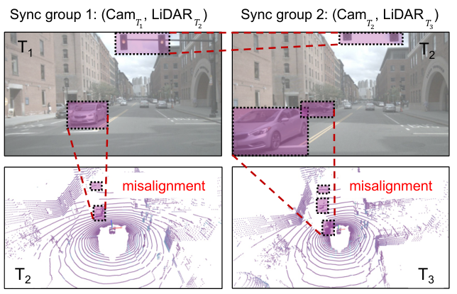
Aligning to low-rate keyframes is not enough. A common workaround is to downsample all inputs to low-rate keyframes. While this reduces the nominal offset, it sacrifices temporal resolution and reaction time, and still leaves residual misalignment once multi-sweep aggregation and real bus jitter are considered. Moreover, coarse, frame-level synchronization ignores where the informative content actually lies (Fig. 2): most camera pixels are low-saliency, so forcing strict frame-level alignment wastes bandwidth and compute on uninformative regions.
Insight 2. Asynchronous sampling routinely introduces – ms offsets between camera and LiDAR. Naively aligned features describe different physical states of the world, producing feature conflicts (ghosting, mismatched object sets) that degrade fusion accuracy.
III-C Why Criticality?
Most detected objects are safety-noncritical. Standard BEV evaluation measures recall over all annotated objects—pedestrians 50 m behind the ego, traffic cones on the opposite shoulder, parked vehicles far outside any plausible collision path. These objects contribute equally to mAP, yet a planner would not alter its immediate control action for any of them. To quantify this structure, we classify each annotated object as mandatory or optional based on the ego’s driving state: an object is mandatory if it lies inside the ego’s forward braking distance or its time-to-collision falls below a per-class threshold, and optional otherwise (formalized in §IV-C). Applying this classifier to all annotations across the nuScenes v1.0-mini scenes, Fig. 6 shows that only of all annotations are mandatory; the remaining are optional. The mandatory fraction varies by class—motorcycles () and construction vehicles () are most likely to be in the ego’s path, while barriers () and traffic cones () rarely are—but no class exceeds one third of its annotations being mandatory.

Insight 3. An overwhelming majority of annotated objects ( on nuScenes) fall outside the ego’s braking envelope and short-TTC window, so they are irrelevant to the planner’s immediate control action. All-object recall therefore conflates two very different costs: dropping an optional far-field object is safety-neutral, while dropping a mandatory in-path object is not. Real-time BEV perception must be designed and measured against the mandatory subset.
IV System Design
This section details the design of MM-BEV. Building on the three insights of Section III, MM-BEV routes both modalities’ compute through fine-grained ROIs (addressing the spatial/temporal redundancy of Insight 1), treats synchronization and detection as a joint problem to mitigate the inter-modal timing offsets we measured (Insight 2), and decomposes perception into a mandatory part — the safety-critical detections a planner must act on this cycle — and an optional part (Insight 3), prioritizing the mandatory part for low-latency completion and shedding optional work when the compute budget is tight. We first give an overview, then state the technical challenges, then detail each component.
IV-A System Overview
Fig. 7 depicts the architecture of MM-BEV. Unlike the conventional pipeline of Fig. 1, which densely extracts features from every frame, MM-BEV routes compute by where it matters and when it matters. It begins with a criticality-ranked temporal-ROI selector : rather than re-scanning each frame, it projects the previous frame’s motion-extrapolated detections into per-modality regions of interest (ROIs) and ranks them by criticality, so the mandatory set is always covered while redundant coverage is dropped. A synchronization module assembles the raw sensor data for the selected ROIs from a buffer and motion-compensates multi-sweep LiDAR to a common reference time. The camera branch performs sparse ROI-aware feature extraction , running the backbone only on a shared-shape ROI crop at a context-adaptive resolution; the LiDAR branch uses ROI-aware voxelization , voxelizing only the ROI point set. At the core, a latency-aware coordinator holds the per-frame budget — scheduling the LiDAR sweep window, the image resolution, and periodic full-scene keyframes from scene dynamics and time-to-collision (TTC) — and runs the whole pipeline under an asynchronous producer/consumer scheduler so the model always consumes the freshest synchronized sensor bundle.
IV-B Technical Challenges
MM-BEV is designed to address four challenges in achieving efficient and accurate BEV perception with real-time latency.
C1: Modeling where compute matters. How can the scene be modeled to route compute to the regions that matter, without missing safety-critical objects? MM-BEV exploits temporal coherence — the previous frame’s detections, constrained by physical motion, localize this frame’s objects — and ranks the resulting ROIs by criticality derived from ego state, so the mandatory set is never dropped.
C2: Mitigating sensor misalignment. How can temporal misalignment across asynchronous sensors be minimized? MM-BEV forms ROI-guided synchronization groups and motion-compensates multi-sweep LiDAR to a common reference time before fusion.
C3: Processing sparse, variable-sized inputs. How can feature extraction handle sparse ROIs efficiently on encoders built for dense inputs? MM-BEV runs the camera backbone on a shared-shape ROI crop at a context-adaptive resolution and confines LiDAR voxelization to the ROI point set — limiting computation to informative regions without padding waste.
C4: Keeping latency low. How can the latency–accuracy trade-off be managed so the pipeline sustains real-time rates? A latency-aware coordinator schedules keyframes, the LiDAR sweep window, and image resolution from scene dynamics and TTC, and an asynchronous scheduler keeps end-to-end latency low by always running on the freshest sensor bundle.
IV-C Criticality-Ranked Temporal-ROI Selector
The selector reduces redundant computation by extracting sparse, semantically critical regions from raw sensor data. It rests on two ideas: temporal localization — the previous frame tells us where objects are — and criticality ranking — which of those regions are mandatory.
Temporal ROI localization. Object motion between consecutive frames is physically bounded, so the previous frame’s detections are a reliable prior for the current frame. Let be the set of boxes detected at frame , each carrying an estimated velocity . MM-BEV projects every box forward by and forms per-modality ROIs from the union of current and motion-extrapolated box footprints. For the LiDAR branch, ROIs are axis-aligned BEV bounds buffered by a margin :
| (1) |
For the camera branch, the same box set is projected to each image plane and expanded by pixels for localization uncertainty:
| (2) |
The image ROIs across all cameras are normalized to a single shared shape (§IV-E) so the backbone forward is batched without padding waste; cameras with no projected box receive a small fallback crop. When the cache is empty (first frame, or after a keyframe), the selector falls back to the full-frame pipeline.
Criticality model. Not every detected object carries equal real-time value. MM-BEV scores each object from the ego state — speed and heading — and the object’s geometry, into two classes. For an object with relative position ( forward of the ego, lateral) and class , the object is geometry-critical if it lies within the ego’s forward braking cone:
| (3) |
with braking distance
| (4) |
where is the forward-cone half-angle at the current ego speed, is a nominal deceleration, and a floor for low-speed proximity. The object is safety-critical if its time-to-collision (§IV-G, Eq. 8) falls below a per-class threshold :
| (5) |
with tighter for vulnerable road users than for static objects. The mandatory set is the union ; the rest is optional. Criticality ranks the ROIs: the selector guarantees coverage of mandatory ROIs at full fidelity and is free to shrink, down-sample, or drop optional ROIs to hold the latency budget (§IV-G). The criticality model is also the basis of the evaluation metric (§VI), which measures accuracy on the mandatory set rather than over all objects.
Criticality thresholds. The forward-cone half-angle is a piecewise-linear function of ego speed: it widens at low speed (where lateral maneuvers are still possible) and narrows at highway speed (where the relevant corridor is forward and narrow), bounded between and . Per-class TTC thresholds are set conservatively: s for vulnerable road users (pedestrians, cyclists) and s for motorized objects; static infrastructure (barriers, cones) is treated as geometry-critical only, since their relative velocity is zero and TTC is undefined. These values are tunable deployment parameters matched to typical highway-code reaction-distance requirements.
IV-D Synchronization
Synchronization integrates sensor data across time and space. MM-BEV treats synchronization and fusion as one module, aligning data temporally and spatially before fusion.
ROI-guided sync groups. Not all sensor data is equally informative at every timestep [yan2023cross]. MM-BEV adapts the synchronization group from ROI information rather than always fusing all six cameras and LiDAR [liu2024rt], and occasionally promotes a comprehensive keyframe involving all sensors (§IV-G). The synchronization window is set from the ego speed and TTC.
Motion compensation. Aggregating multiple LiDAR sweeps introduces time differences that misalign points [xia2025robust], as shown in Figs. 3 and 5. MM-BEV compensates with the ego motion between sweep timestamps: a point from an earlier sweep at is transformed to the current frame as
| (6) |
and the current sweep is aggregated with motion-compensated previous sweeps,
| (7) |
where is the sweep count chosen by the coordinator (§IV-G). Fig. 8 illustrates the effect on a nuScenes scene with ego motion across the sweep window: without compensation, static structures appear as several ghost copies offset along the direction of travel; with compensation, the same structures collapse to a single coherent position.

IV-E Sparse ROI-Aware Camera Feature Extraction
Image ROIs occupy only a small fraction of the dense image, so the camera backbone should not process every pixel.
Shared-shape ROI crop. MM-BEV crops each camera to its ROI window and normalizes all crops to a single shared shape , sized from the largest projected ROI and snapped to the backbone stride. Per-camera offsets place each crop; cameras with no ROI get a small center crop. Because all crops share a shape, the backbone forward is a single batched pass with no padding waste. After the backbone and neck, the cropped features are pasted onto a full-image feature canvas at the correct stride, and a binary ROI mask marks the pasted region. The mask is carried into the view transform and zeroes the BEV contribution of canvas regions that held no real features, removing the camera-side accuracy floor that a zero-padded canvas would otherwise introduce.
Context-adaptive resolution. The camera backbone is the dominant cost in the image branch. MM-BEV runs it at a context-adaptive resolution: when the scene is slow and sparse, the ROI crop is downsampled before the backbone and the features are upsampled back, halving the image backbone cost; when the scene is fast and dense, full resolution is kept. The resolution choice is made per frame by the coordinator (§IV-G).
IV-F ROI-Aware Voxelization
LiDAR point clouds are sparse, yet conventional pipelines voxelize the whole space and run sparse convolutions over every non-empty voxel, including regions of little semantic value [liu2023bevfusion]. MM-BEV confines LiDAR processing to the ROIs.

As in Fig. 9 and Alg. 1, MM-BEV keeps points by their position relative to : points inside the (motion-padded) ROI box union are kept in full, and points outside are kept at a reduced rate, so most of the background is dropped while the ROI neighborhood — including localization slack — is preserved. The retained points are voxelized and passed through the Voxel Feature Encoder; features are scattered into a zero-initialized BEV map by voxel coordinate. The result has the same BEV shape as a dense pipeline but is computed from a focused subset of points, cutting LiDAR cost without sacrificing coverage of critical regions.
LiDAR latency scales with voxel count. We confirm that reducing the voxel count translates directly into inference-time savings. We profile the BEVFusion LiDAR-only branch on nuScenes scenes, sub-sampling each point cloud at rates to generate a range of voxel counts after hard voxelization, and time each LiDAR stage on the RTX 3080. Across runs (Fig. 10), the total LiDAR latency is well-modeled by a linear fit ms (), where is the non-empty voxel count in thousands. The breakdown shows that voxelization and the sparse encoder grow nearly linearly with , while the SECOND backbone and FPN neck stay constant at ms. A full-resolution sweep yields k voxels and ms; restricting compute to the ROI brings to k and the LiDAR cost to ms—a saving on this stage alone.
IV-G Latency-Aware Coordinator
The coordinator holds the per-frame latency budget. It does so along two axes: compute scaling — adjusting how much work each frame does — and pipeline scheduling — ensuring the model always runs on fresh data.
Time-to-collision. The coordinator’s signals come from ego/object motion. Given an obstacle’s relative position and velocity , the time of closest approach is
| (8) |
and if and , else . The minimum TTC over the scene drives both the safety-criticality test (§IV-C) and the coordinator’s budget decisions.
Priority-based budget management. The coordinator has two compute knobs—the LiDAR sweep count and the image resolution—and applies them in priority order. Mandatory-ROI coverage is fixed first and cannot be shed. The sweep count is reduced next, from at high ego speed down to when the ego is slow or the scene is dense (recent frames already carry the needed context). Image resolution is dropped last, to half when the scene is slow and sparse and kept full otherwise. If the minimum configuration still risks running long, the coordinator falls back to LiDAR-only inference for that frame, preserving the mandatory LiDAR-ROI path while shedding the camera branch entirely. Both knobs trade optional fidelity for latency and never touch the mandatory ROIs; on the evaluation platform, the half-resolution ROI path consistently fits within the ms per-frame target.
Keyframes. ROI-based perception risks error accumulation and stale context, since newly appearing objects have no temporal precedent. MM-BEV periodically inserts a keyframe — a full-scene pass that refreshes the detection cache and bounds the worst-case staleness of the temporal prior. The keyframe interval may be fixed or triggered by scene dynamics: MM-BEV estimates the per-frame ROI change
| (9) | ||||
| (10) |
where is a LiDAR-ROI area and an ego-motion-compensated camera-ROI centroid; a keyframe is forced when either exceeds a profiled threshold.
Asynchronous scheduling. Compute scaling reduces per-frame work, but in a live pipeline it does not by itself bound end-to-end latency: if inference is invoked synchronously inside the sensor callback, frames queue and the detector consumes ever-staler data. MM-BEV runs the pipeline as a producer/consumer pair: the sensor callback only buffers the latest synchronized bundle and returns immediately, while a separate inference thread always consumes the freshest buffered bundle and discards stale ones. With a single-slot buffer, an unbounded backlog becomes a bounded queue and end-to-end latency becomes predictable. Algorithm 2 summarizes the per-frame coordination.
V Implementation
We integrate MM-BEV’s implementation into BEVFusion’s perception pipeline using ROS on a resource-limited GPU desktop [liu2023bevfusion, quigley2009ros]. BEVFusion is a widely deployed baseline for multi-modality BEV perception [liu2023bevfusion, liu2021swin, xie2023sparsefusion, bai2022transfusion, liang2022bevfusion].
ROS framework. To emulate real-time streaming processing similarly to actual AVs, we implement MM-BEV using ROS [quigley2009ros, message-filter], as depicted in Fig. 11. Specifically, we develop three ROS nodes: Sensor Publisher, Synchronizer, and Detector. The Sensor Publisher publishes ROS bags generated from nuScenes dataset, incorporating raw sensor data (6 cameras and 1 LiDAR) alongside CAN bus information from the ego vehicle. Camera frames are published at 12 Hz, while LiDAR data is published at 20 Hz. The Synchronizer node consists of a Sweep Buffer that caches previous LiDAR sweeps, a Transform module for precomputing metadata containing sensor coordinate transformations (rotation and translation), and a Sync Callback, which serves as the entry point for synchronizing sensor data based on the ROIs within a configurable slop threshold. The Detector node closely follows the design structure of MM-BEV, with minor adaptations for ROS-based inter-module communication using ROS parameters. Specifically, parameters like slop and sync_group are employed by the Coordinator to dynamically adjust synchronization settings. The keyframe parameter also indicates the keyframe mode, and and parameters are used for real-time updates of ROIs for cameras and LiDAR, respectively.
Asynchronous scheduling. The Synchronizer publishes each synchronized bundle to a single-slot topic and returns immediately; the Detector subscribes with queue_size=1 and an overwrite-on-arrival callback, so a bundle arriving while inference is busy replaces the queued one rather than being appended. The Detector thus always consumes the freshest available bundle.
VI Evaluation
We evaluate MM-BEV end-to-end on the nuScenes dataset replayed through ROS and via a controlled offline timing benchmark, then deploy the system on a real robot.
VI-A Experimental Setup
Hardware. Offline timing benchmarks run on a desktop with a 12th-Gen Intel® Core™ i9-12900K (3.3 GHz) and an NVIDIA GeForce RTX 3080 (29.8 TFLOPS FP32, 10 GB GDDR6). End-to-end ROS experiments run on the same machine. Libraries: CUDA 12.3, PyTorch 2.4.1, mmdet3d 1.2.0, ROS Noetic.
Dataset. We use the nuScenes dataset [caesar2020nuscenes]: 11,628 images (1600928, 6 cameras) plus 20-sweep LiDAR, covering 10 driving scenes. In the ROS experiments, camera frames are published as sensor_msgs/Image at 12 Hz and LiDAR as sensor_msgs/PointCloud2 at 20 Hz.
Baselines and configurations. Table I lists all evaluated configurations. BEVFusion [liu2023bevfusion] is the primary baseline (dense, full-resolution, synchronous pipeline). Scheduler Only adds the asynchronous streaming scheduler alone, without ROI or adaptive resolution. Ablation variants progressively add ROI routing, adaptive sweep count, and adaptive (or fixed low) image resolution. MM-BEV is the full proposed system.
| Config | Sensors | Temporal ROI | Adaptive res. | Async sched. |
|---|---|---|---|---|
| BEVFusion [liu2023bevfusion] | L+C | × | × | × |
| Scheduler Only | L+C | × | × | ✓ |
| ROI | L+C | ✓ | × | × |
| ROI+LowRes | L+C | ✓ | fixed-low | × |
| ROI+Adapt+LowRes | L+C | ✓ | adaptive | × |
| MM-BEV | L+C | ✓ | adaptive | ✓ |
| MM-BEV+LowRes | L+C | ✓ | fixed-low | ✓ |
Metrics. We report inference latency (mean over non-warmup frames, split by keyframe vs. ROI-frame mode), end-to-end latency (sensor exposure to detection output, measured in ROS), processed frames per scene, and criticality-bucketed recall: all-object recall, geometry-critical recall (objects inside the ego braking cone), and safety-critical recall.
VI-B Inference Latency
Fig. 12 compares per-frame inference latency for the fusion and LiDAR-only detectors. MM-BEV classifies every frame as either a keyframe (full inference, triggered periodically or by high scene dynamics) or a ROI frame (inference restricted to the temporal ROI).
Fusion detector. The baseline must run full-resolution, full-sweep inference on every frame: 202 ms per keyframe and 118 ms per “ROI frame” (the baseline uses adaptive sweeps but no ROI crop). MM-BEV cuts the ROI-frame cost to 104 ms (a 1.96 speedup over the baseline keyframe), while keyframe cost stays at 216 ms due to the shared-shape crop overhead. With a keyframe interval of (the default), the ROI frames are the common case and dominate the average.
LiDAR-only detector. The baseline keyframe costs 136 ms; MM-BEV ROI frames cost 70 ms (1.94). The LiDAR path benefits less from ROI-based voxelization because point clouds are already sparse; the main gain comes from the adaptive sweep window.
Fig. 13 shows the stage-level breakdown for the fusion detector. Image feature extraction is the dominant lever: the full-resolution backbone takes 57 ms; temporal ROI with low-resolution input cuts it to 21 ms (2.7). LiDAR feature extraction (84 ms baseline) contracts only modestly under ROI voxelization (83–91 ms), consistent with its already-sparse structure. The BBox head and fusion stage together account for only 12 ms and are invariant across configurations.
VI-C Criticality-Bucketed Accuracy
Fig. 14 shows all-object, geometry-critical, and safety-critical recall for the key configurations.
Geometry-critical recall is preserved exactly. Every ROI-based configuration matches the baseline at on geometry-critical objects. This is by construction: the criticality-ranked selector (§IV-C) always covers the mandatory set derived from the ego’s braking cone, so no object inside that zone is skipped.
Safety-critical recall degrades minimally. Safety-critical recall (objects below the per-class TTC threshold) drops pp for MM-BEV ( vs. baseline ) and at most pp for MM-BEV+LowRes (). The small loss reflects the part of the safety-critical set that lies just outside the braking cone and is therefore not covered by the geometry ROI.
All-object recall drops only on optional objects. All-object recall falls pp for MM-BEV and pp for MM-BEV+LowRes; in both cases the lost detections are entirely in the optional set (distant, low-TTC background traffic), so the conventional all-object mAP exaggerates the safety impact of these ROI/resolution trade-offs.
| Config | Per-frame lat. (ms) | All-obj R (%) | Geom-crit R (%) | Safety-crit R (%) |
|---|---|---|---|---|
| BEVFusion | 202 | 79.9 | 100.0 | 94.9 |
| ROI+Adapt+LowRes | 95 | 78.4 | 100.0 | 95.2 |
| MM-BEV | 104 | 79.5 | 100.0 | 94.7 |
| MM-BEV+LowRes | 92 | 77.6 | 100.0 | 94.2 |
| LiDAR Baseline | 136 | 76.8 | 100.0 | 93.5 |
| LiDAR MM-BEV | 70 | 76.8 | 100.0 | 93.1 |
Table II summarizes the latency–accuracy trade-off. MM-BEV+LowRes achieves the best per-frame latency ( ms, faster than the ms full-inference baseline) while holding geometry-critical recall at and dropping safety-critical recall by only points.
VI-D Ablation Study
Latency–accuracy trade-off. Fig. 15 places all ablation configurations in the latency–recall plane, with each system at its per-frame cost in the common-case operating mode (full inference for the baseline; ROI-frame inference for ROI/MM-BEV variants). Three conclusions follow. (i) ROI alone provides limited camera savings (ROI: ms ROI-frame vs. baseline: ms full-inference)—the ROI crop reshapes computation but does not reduce image resolution, so the backbone still pays for full-resolution features. (ii) Low resolution is the primary camera lever (ROI+LowRes: ms; MM-BEV+LowRes: ms ROI-frame): cutting image input from to slashes image feature extraction from ms to ms. (iii) Adaptive resolution (MM-BEV: ms ROI-frame) keeps full resolution when scene dynamics demand it but drops to half-res on slow/sparse scenes, maintaining all-object recall points above the always-low-res variant at the cost of ms higher ROI-frame latency.
LiDAR ablation. Fig. 16 sweeps LiDAR-only variants. ROI-based voxelization alone marginally increases the keyframe cost (from 136 to 129 ms for LiDAR-ROI), since the region selection adds a preprocessing step without proportionally reducing the point set on keyframes. Adaptive sweep count (ROI+Adapt and MM-BEV) recovers this overhead, settling at 100 ms mean—a modest 1.03 improvement. All-object and safety-critical recall are stable across all LiDAR configurations (76.8% and 93%, respectively), confirming that the sweep-count reduction does not degrade detection quality.
VI-E End-to-End Pipeline Performance
Fig. 17 evaluates the full pipeline in ROS, including communication, synchronization, inference, and queuing.
Scheduler dominates the e2e gain. The baseline pipeline stalls on its synchronous queue: camera and LiDAR messages pile up while the detector runs at 1006 ms e2e latency, processing only 10 frames per scene. Scheduler Only—which adds the asynchronous producer/consumer pipeline but no ROI—already cuts e2e latency to 371 ms and raises throughput to 56 frames. This confirms that backlog growth behind the synchronous detector is the main bottleneck in the baseline.
Full MM-BEV. Adding temporal ROI and adaptive resolution (MM-BEV) reduces e2e latency further to 344 ms (a 2.93 reduction over baseline) and processes 60 frames per scene (a 6 improvement). The per-frame detection contribution drops from 199 ms (baseline model) to 95 ms (MM-BEV model), consistent with the offline benchmarks in §VI-B.
| Config | Frames/scene | E2E lat. mean (ms) | E2E lat. p95 (ms) | Speedup |
|---|---|---|---|---|
| BEVFusion | 10 | 1006 | 1455 | – |
| Scheduler Only | 56 | 371 | 498 | |
| MM-BEV | 60 | 344 | 434 |
Table III provides the full numbers. The 95th-percentile e2e latency shrinks from 1455 ms to 434 ms, confirming that the long tail of the backlog—not just the average—is reduced. The residual gain from ROI on top of the scheduler alone (371 to 344 ms) reflects faster per-frame model execution translating to a shorter queue wait time.
VI-F Real-World Deployment

Platform. We validate MM-BEV on a Clearpath Husky A300 mobile robot [clearpath_huskya300] equipped with six e-con AR0234 GMSL2 wide-angle cameras (, HFOV) [econ_ar0234] and an Ouster OS1-128 LiDAR [ouster_os1]; all perception runs on the onboard NVIDIA Jetson AGX Orin with the BEVFusion backbone compiled to TensorRT int8. We collect a -minute drive ( frames) across outdoor plazas, parking lots, and indoor corridors. The dense baseline runs full inference every frame at a mean ms; a lightweight voxel-grid connected-component proposer identifies object clusters in ms ( faster than sklearn DBSCAN at ms).

Adaptive scheduler. The scheduler picks a per-frame keyframe interval from the robot’s odometry speed and the inter-frame BEV cluster shift (Fig. 20): when stationary (trigger “speed”), and when the cluster set changes between frames during active driving (trigger “cluster-shift”). Across the drive the scheduler selects with of frames as keyframes, yielding a mean per-frame inference latency of ms—a reduction over the dense baseline. By comparison, fixed and reach ms () and ms () but cannot react to scene changes. Fig. 19 shows a representative frame: forward-path vehicles and a crossing pedestrian are all detected on-device, confirming that the temporal-ROI and adaptive-resolution gains transfer from desktop GPU to the constrained Jetson Orin compute budget.
VII Related Work
BEV perception has become mainstream for AVs, thanks to its comprehensive view understanding, which guides their planning and navigation [BEV-Perception-Survey-2024, ma2023visioncentric]. Compared to vision-centric BEV perception that utilizes only camera inputs [li2022bevformer, yang2023bevformer, hu2023planning], multi-modality BEV perception combining LiDAR and cameras is more practical and widely deployed, primarily due to its superior accuracy and reliability across diverse traffic scenarios [liang2022bevfusion, liu2023bevfusion].
However, achieving real-time BEV perception remains challenging due mainly to the high computational demands from high-frequency and high-resolution multi-modality sensors [liu2023bevfusion]. SOTA research has primarily approached this challenge by either designing lightweight models or compressing dense models into sparse structures to improve computational efficiency [xie2023sparsefusion, bai2022transfusion, yan2023cross]. For instance, BEVFusion [liu2023bevfusion] utilizes dense camera and LiDAR feature maps to perform sensor fusion within a shared BEV space. Transfusion [bai2022transfusion] maintains dense features for the camera branch but uses sparse projection for LiDAR inputs. SparseFusion [xie2023sparsefusion] employs sparse features and fusion to reduce overhead. Cross-Modality Transformer (CMT) [yan2023cross] further explores efficient multi-modal integration by designing a transformer-based feature transformation. Yet, these methods ignore the inherent sparsity in input sensor data — not all pixels are equally important — or consider redundancy only intra-modality. Remix and Elf recognize the variable importance of regions and but only apply to one camera, not applied directly to multi-modality sensors [zhang2021elf, jiang2021flexible]. FLEX considers BEV cameras but only focuses on frame-level ROIs [xu2024flex]. MMEdge [huang2026mmedge] pipelines on-device multimodal inference by overlapping sensing and encoding into fine-grained units with cross-modal speculative skipping, but operates on classification-style fusion tasks rather than dense BEV detection. Another challenge is cross-modal synchronization: LiDAR and cameras operate at different frequencies, and poor alignment of their data can degrade performance. RT-BEV [liu2024rt] tackles the ROI and synchronization issues of cameras only. MM-BEV extends it to a more practical LiDAR–camera combination, leveraging both input sparsity and robust alignment for efficient BEV perception.
VIII Conclusion
We presented MM-BEV, a real-time multi-modality BEV perception system organized around the principle of computing where and when it matters. MM-BEV decomposes BEV detection into a mandatory part—the critical objects inside the ego’s braking distance and short time-to-collision—and an optional part, and combines four mechanisms (a criticality-ranked temporal-ROI selector, sparse ROI-aware feature extraction, a latency-aware coordinator, and an asynchronous streaming scheduler). On nuScenes—where only of annotated objects are mandatory under the criticality model—MM-BEV cuts inference latency by and end-to-end latency by , preserves geometry-critical recall exactly, and drops safety-critical recall by only percentage points. On a Clearpath Husky A300 robot with Jetson AGX Orin, MM-BEV reaches a further mean-latency reduction under an adaptive keyframe schedule, confirming that the gains transfer to embedded hardware. These results show that criticality-aware scheduling is a practical foundation for real-time multi-modality perception on resource-limited AVs.