Flexible covariance structures on metric graphs

We refer to a metric graph $\Gamma$ as the pair $\Gamma=(\mathcal{V},\mathcal{E})$, where $\mathcal{V}$ is a set of vertices and $\mathcal{E}$ a set of edges. The edges $e\in\mathcal{E}$ are line segments that are attached in vertices $v\in\mathcal{V}$. We assume that the graph is connected, i.e., there exists a path between any pair of locations on the graph. A location on the graph is represented by the pair $\boldsymbol{\mathbf{s}}=(e,d)\in\Gamma$, where $e\in\mathcal{E}$ identifies the edge and $d\in[0,1]$ gives the normalized position (parametrized by arc length) along edge $e$. We write $\underline{e}=(e,0)$ and $\overline{e}=(e,1)$ for the start and end points of edge $e$, respectively. Since vertices may be shared by multiple edges, a single location can admit multiple coordinate representations. For example, if the end vertex of $e_{2}$ coincides with the start vertex of $e_{1}$, then $\underline{e_{1}}=\overline{e_{2}}$, and both coordinate pairs represent the same spatial location.

The order of a vertex refers to the number of edges connected at the vertex. Note that there are multiple representations of a metric graph where vertices of order 2 can be added and/or removed, and the metric graph remains the same, while the minimal set of edges and vertices that represent the same geometry, is referred to as the minimal graph. Let $\lvert\mathcal{V}\rvert$ denote the number of vertices in the metric graph. Vertices of degree 1 are called terminal vertices, and vertices of order 2 or greater are internal vertices.

A key component in extending the “SPDE approach” to metric graphs is to define a Laplacian, $\Delta_{\Gamma}$, on the metric graph. In our context, it is enough to define it almost everywhere, and we define it as a normal second-order derivative with respect to arc length on the internal points of the edges. However, under this definition, there is no unique inverse, and thus no unique solution to SPDE (1). Heuristically, this can be resolved by choosing that $\Delta_{\Gamma}^{-1}f$ for $f\in L_{2}(\Gamma)$ should be a function that is continuous at all vertices and where the directional derivatives sum to zero at all vertexes. 6 gives a mathematical description of this Kirchhoff-Laplacian.

We give a overview of model definition, parameterization, discretization, and computations in this section, but refer the reader to 6, 8, 4 for technical details and more formal conditions on the coefficients for WM-GRFs and GWM-GRFs, and 18 for a more practical introduction for WM-GRFs. This section focuses on known material described in an accessible way, and Section 2.3 focuses on the novel contributions in this paper.

Gaussian white noise, $\mathcal{W}(\cdot)$, extends in a straightforward way to a metric graph $\Gamma$ by measuring the sizes of sets using arclength, and the GWM-GRFs are defined as solutions to

where $\Delta_{\Gamma}$ is the Kirchhoff-Laplacian, and $\kappa(\cdot)>\kappa_{0}>0$ and $\tau(\cdot)>\tau_{0}>0$ are real functions on $\Gamma$. Note that $\mathcal{W}(\cdot)$ is an abuse of notation, as point-wise evaluation of the noise process is not defined. The parameter $\alpha>1/2$ is assumed to be fixed and determines the smoothness of the solution $u(\cdot)$. At terminal vertices (i.e., vertices of order 1), solving with the Kirchhoff-Laplacian implicitly imposes zero Neumann boundary conditions.

As discussed in the introduction, WM-GRF is not an approximation of a Matérn GRF on the metric graph, as the Matérn covariance function is, in general, not valid when geodesic distances are used. The covariance structure must be understood as a generalization to the non-Euclidean geometry that locally behaves similarly as the Matérn, in the sense that it satisfies the same SPDE as it would in 1D together with vertex conditions to combine the different 1D segments together. Unlike a Matérn GRF in the usual Euclidean case, a WM-GRF does not have a constant marginal variance $\sigma^{2}(\kappa,\tau,\alpha)$ and a constant practical correlation range $\rho(\kappa,\alpha)$. A similar effect is found for bounded Euclidean domains where the boundary conditions affect the covariance structure in the vicinity of the boundary. This motivates us to avoid the imprecise terms stationary and non-stationary, and use WM-GRF for constant coefficients and GWM-GRF for spatially-varying coefficients.

Inspired by 20, 4 propose using log-regressions for the spatially varying coefficients,

where $p^{\kappa},p^{\tau}\in\mathbb{N}$ denotes the numbers of basis functions, $\{\xi_{1}^{\kappa}(\cdot),\ldots,\xi_{p^{\kappa}}^{\kappa}(\cdot)\}$ and $\{\xi_{1}^{\tau}(\cdot),\ldots,\xi_{p^{\tau}}^{\tau}(\cdot)\}$ are known real-valued basis functions, and the coefficients $b_{1}^{\kappa},\ldots,b_{p^{\kappa}}^{\kappa}\in\mathbb{R}$ and $b_{1}^{\tau},\ldots,b_{p^{\tau}}^{\tau}\in\mathbb{R}$ are model parameters. For $p^{\kappa}=p^{\tau}=1$ and $\xi^{\kappa}(\cdot)=\xi^{\tau}(\cdot)\equiv 1$, this gives a WM-GRF. For small $p^{\kappa}$ and $p^{\tau}$, and $\xi^{\kappa}(\cdot)$ and $\xi^{\tau}(\cdot)$ defined as covariates, this gives GWM-GRFs where covariance structure is described by a few spatial covariates. Finally for large $p^{\kappa}$ and $p^{\tau}$, this gives GWM-GRFs with a very flexible covariance structure. The two former models have been detailed in existing literature, while the latter is novel and is explained in Section 2.3.

Computations with WM-GRFs on metric graphs are based on extending the finite element method (FEM) approach of 20 from Euclidean domains to metric graphs. The FEM representation leads to sparse element matrices and, consequently, sparse precision matrices, which provide the Markov properties exploited for efficient computation. The key idea is to use the fact that each edge is locally one-dimensional and to seek a weak solution to (2) that is compatible across the graph. In the simplest case, where the graph consists of a single edge connecting two terminal vertices, the solution coincides with the classical one-dimensional Matérn Gaussian random field (up to boundary effects). We fix $\alpha=2$ for the rest of the paper, which gives a smoothness of $1.5$ so that GRF is once differentiable, everywhere except the vertices, and the derivative is a GRF with smoothness $0.5$. The conditions on the inverse of $\Delta_{\Gamma}$ ensures that, for each vertex, the GRF $u(\cdot)$ is continuous and that the directional derivatives sum to zero.

To apply FEM, we discretize the metric graph by constructing a mesh. This is done, by adding vertices to edges that are longer than a certain maximal mesh spacing $h>0$. For an edge with length larger than $h$, new vertices are inserted recursively until all resulting sub-edges have lengths no greater than $h$. The resulting metric graph, consisting of the original vertices together with the additional mesh vertices, is referred to as the mesh. The mesh is “the same” metric graph as originally, but not the minimal description without vertices of order 2. Critically, 6 show that adding a vertex, of order 2, to an edge does not change the solution $u(\cdot)$. Let $\mathcal{V}_{h}\supseteq\mathcal{V}$ be the set of vertices in the mesh and $m_{h}=\lvert\mathcal{V}_{h}\rvert$. We refer to Figure 1 for an illustration of a simple metric graph with two meshes of different coarseness $h$.

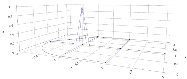
Given the mesh with maximal spacing $h$, we define the set of linear basis functions $\{\psi_{h,j}(\cdot)\}_{j=1}^{m_{h}}$ as the collection of piecewise linear functions that satisfy $\psi_{h,j}(v_{i})=1$ if and only if $j=i$ and zero otherwise for a graph or mesh vertex $v_{i}\in\mathcal{V}_{h}$. Such set can be defined for any mesh on a graph $\Gamma$. The number of basis functions is equal to the number of vertices, $m_{h}$, in the mesh. Figure 2 illustrates one basis function on a simple graph.

The FEM approach to obtain the weak solution to (2) on $\Gamma$ with spatially varying $\kappa(\boldsymbol{\mathbf{s}})$ and $\tau(\boldsymbol{\mathbf{s}})$ was introduced by 4. In the following we provide a short introduction here, and refer the reader to 4 for full derivation. We approximate the solution $u(\cdot)$, on a mesh with vertices $\mathcal{V}_{h}$, using the finite-dimensional representation

where $\psi_{h,j}(\cdot)$ for $j=1,\ldots,m_{h}$ are piece-wise linear basis functions and $m_{h}=|\mathcal{V}_{h}|$. The weak formulation is obtained by requiring that,

By the divergence theorem, and assuming Neumann boundary conditions for $u_{h}(\cdot)$ and $\tau(\cdot)$ (the derivatives are zero at the boundary/terminal vertices), we end up with the following equality for each row

for all $k=1,\ldots,m_{h}$. We can define element matrices $\boldsymbol{\mathbf{C}}_{h}=[\langle\psi_{h,i},\psi_{h,j}\rangle]_{ij}$, $\boldsymbol{\mathbf{C}}_{h}^{\kappa,\tau}=[\langle\tau\kappa^{2}\psi_{h,i},\psi_{h,j}\rangle]_{ij}$ and $\boldsymbol{\mathbf{G}}_{h}^{\tau}=[\langle\nabla(\tau\psi_{h,i}),\nabla\psi_{h,j}\rangle]_{ij}$, where $\langle f,g\rangle$ is integration over all of $\Gamma$, which can be understood as piecewise integration over the collection of edges. In practice, one cannot evaluate the integrals for all elements in the matrices $\boldsymbol{\mathbf{C}}^{\kappa,\tau}_{h}$ and $\boldsymbol{\mathbf{G}}_{h}^{\tau}$. Instead one approximates $C^{\kappa,\tau}$ by combining a lumped mass matrix $\boldsymbol{\mathbf{C}}_{h}$ and diagonal matrices of $\kappa(\cdot)$ and $\tau(\cdot)$ evaluated in vertices $\mathcal{V}_{h}$. We further obtain the precision matrix for the weights $\boldsymbol{\mathbf{w}}=[w_{1}\>\ldots\>w_{m_{h}}]^{\mathrm{T}}$, given by

Note that, for spatially constant coefficients in (2), $\kappa(\boldsymbol{\mathbf{s}})=\kappa$ and $\tau(\boldsymbol{\mathbf{s}})=\tau$ for all $\boldsymbol{\mathbf{s}}\in\Gamma$, the precision matrix simplifies to

where $\boldsymbol{\mathbf{G}}_{h}=[\langle\nabla(\psi_{h,i}),\nabla\psi_{h,j}\rangle]_{ij}$ and still $\boldsymbol{\mathbf{C}}_{h}=[\langle\psi_{h,i},\psi_{h,j}\rangle]_{ij}$.

A common way to specify the spatially varying $\kappa(\boldsymbol{\mathbf{s}})$ and $\tau(\boldsymbol{\mathbf{s}})$, introduced in 17 for Euclidean domains and later tested for metric graphs by 4, is to parameterize the coefficient fields through spatial covariates. Specifically:

where $\boldsymbol{\mathbf{z}}^{\kappa}(\cdot)$ and $\boldsymbol{\mathbf{z}}^{\tau}(\cdot)$ are known covariates defined over the entire graph. The choice of covariates is important, as appropriately selected covariates can provide an interpretable representation of the sources of non-stationarity. For example, altitude covariates can be used to explain spatial variation in rainfall patterns, as demonstrated by 17. When covariate information is only available at a finite set of locations rather than throughout the entire domain, 4 propose covariate smoothing methods to obtain spatially continuous coefficient fields.

Our goal is to introduce an alternative and more flexible way to define covariance structures for the field defined in (3). In the following, inspired by 20, we reparameterize our model as:

where we have assumed smoothness $\alpha=2$ ($d=1$, $\nu=1.5$). In the Euclidean case, $\rho$ and $\sigma$ can be interpreted as the practical range and the marginal variance of the Matèrn field. In the metric graph setting, $\rho(\cdot)$ and $\sigma(\cdot)$ should be interpreted as approximate correlation range and marginal standard deviation parameters due to the influence of graph topology and vertex conditions on the covariance structure. Note that the transformation is linear in log scale, hence inference can equivalently be performed in terms of either parameterization.

To model spatially varying coefficients $\rho(\cdot)$ and $\sigma(\cdot)$, we introduce two coefficient meshes on the graph with maximal edge length $\tilde{h}_{\rho}$ and $\tilde{h}_{\sigma}$ respectively. Denote the corresponding sets of mesh vertices by $\mathcal{V}_{\tilde{h}_{\rho}}$ and $\mathcal{V}_{\tilde{h}_{\sigma}}$ and the numbers of vertices by $m_{\tilde{h},\rho}$ and $m_{\tilde{h},\sigma}$ respectively.

The spatially varying coefficient fields are then represented as

where $\{b_{j}^{a}\}_{j=1}^{m_{\tilde{h}}}$ for $m_{\tilde{h}}=m_{\tilde{h},\rho},m_{\tilde{h},\sigma}$ are the weights associated with the two coefficient fields.

To use this flexible parameterization of $\rho(\cdot)$ and $\sigma(\cdot)$ appropriate priors or penalization terms must be assigned to the coefficients $b_{j}^{\rho}$, $j=1,\ldots,m_{\tilde{h},\rho}$, and $b_{j}^{\sigma}$, $j=1,\ldots,m_{\tilde{h},\sigma}$ to avoid over-fitting. Highly flexible models may fit well to the data, but behave poorly when used for predictions either in unobserved locations or of future observations. On the other side, overly restrictive models may fail to capture more advanced spatial dependencies. Therefore, a balance between model flexibility and regularization is required. From here on, we will only consider $\mathcal{V}_{\tilde{h}_{\rho}}=\mathcal{V}_{\tilde{h}_{\sigma}}$ and $m_{\tilde{h},\rho}=m_{\tilde{h},\sigma}=m_{\tilde{h}}$ and the maximal distance between mesh vertices be $\tilde{h}$. The sets of basis functions become a shared set $\{\varphi_{\tilde{h},j}\}_{j=1}^{m_{\tilde{h}}}$.

We force some relatedness between the coefficients $\{b^{\rho}_{j}\}_{j}$ and between $\{b^{\sigma}_{j}\}_{j}$ by using the same approach suggested by 12. Let $p(\cdot)$ be a GRF defined on a graph $\Gamma$ (it can be either $\log\rho(\boldsymbol{\mathbf{s}})$ or $\log\sigma(\boldsymbol{\mathbf{s}})$), which can be represented as the solution to an SPDE. First, let $p(\cdot)$ be described as follows

where $p_{0}$ refers to the level and $\varphi_{\tilde{h},j}(\cdot)$, $j=1,\ldots,m_{\tilde{h}}$, are piecewise linear basis functions on the mesh with maximal spacing $\tilde{h}$. To ensure identifiability of $p_{0}$ we add a sum-to-zero constraint on $\{b^{p}_{j}\}_{j=1}^{m_{\tilde{h}}}$. We choose $p(\boldsymbol{\mathbf{s}})$ as the weak solution to a SPDE of the form

where $\mathcal{W}_{p}(\boldsymbol{\mathbf{s}})$ is Gaussian white noise without the 0-frequency. See Appendix A for more details on this. The precision matrix of the vector $[b^{p}_{1}\>\ldots\>b^{p}_{m_{\tilde{h}}}]^{\mathrm{T}}$ is given by

where $\boldsymbol{\mathbf{C}}_{\tilde{h}}$ and $\boldsymbol{\mathbf{G}}_{\tilde{h}}$ are element matrices related to the discretization of $\Gamma$ with maximal distance between vertices $\tilde{h}$ and the basis $\{\varphi_{i}(\boldsymbol{\mathbf{s}})\}_{i=1}^{m_{\tilde{h}}}$. These matrices are easy to compute, and are only non-zero in neighboring elements where basis functions are both non-zero. This matrix has null vector $\mathbf{1}$, and is not invertible and therefore not a valid covariance structure. To handle this, we suggest a modified precision matrix

where $\tau_{1}$ and $\tau_{2}$ are penalty parameters, ($\boldsymbol{\mathbf{\tau}}=[\tau_{1}\>\tau_{2}]^{\mathrm{T}}$) to obtain penalization for the complexity of the fields, $\log\rho(\cdot)$ and $\log\sigma(\cdot)$. The interpretation of $\tau_{1}$ is that increasing $\tau_{1}$, also increases the relatedness between neighboring elements, and increasing $\tau_{2}$ means that we force the field to zero (we increase precision for each coefficient and the relatedness between them). In practice, the value of $\tau_{1}$ is the parameter that needs to be tuned for, while minor changes in $\tau_{2}$ does little to the prior/penalization of complex models.

We suggest to tune the penalization parameter $\tau_{1}$ by Monte Carlo simulation with the known distribution of $\boldsymbol{\mathbf{b}}^{f}=[b^{f}_{1}\>\ldots\>b^{f}_{m_{\tilde{h}}}]^{\mathrm{T}}$. By constructing a mesh on the graph with $m_{\tilde{h}}$ vertices, we can draw samples from $\mathcal{N}_{m_{\tilde{h}}}(\boldsymbol{\mathbf{0}},\boldsymbol{\mathbf{Q}}_{\tilde{h},3}^{-1})$, and compute the 95%-quantile for each mesh location, and further evaluate if the range of these quantiles is sufficiently large compared to how much $\log\rho(\cdot)$ and $\log\sigma(\cdot)$ vary in space in our prior knowledge about the log-transformed fields.

Prior information about the practical range can be specified through the implied log-Gaussian distribution of $\rho(\boldsymbol{\mathbf{s}})$. One must have some prior assumption on the mean and variance of $\rho(\boldsymbol{\mathbf{s}})$. Then, one can find the corresponding prior mean and variance of $\log\rho(\boldsymbol{\mathbf{s}})$ through

where $\log(\cdot)$ is the natural logarithm, $\mu_{\rho}$ is the prior mean for $\rho(\cdot)$ and $\sigma^{2}_{\rho}$ is the prior variance. Having prior knowledge of $\mu_{\log\rho}$ and $\sigma_{\log\rho}^{2}$ can then be imposed in tuning for $\tau_{1}$ by ensuring enough variability in the 95%-quantiles.

In practice, we solve (2) using FEM and we choose mesh distance $h$ such that the mesh used for FEM for the latent field $u(\cdot)$ is fine enough to obtain sufficiently accurate results, and the mesh distance $\tilde{h}$ used for basis functions in the covariance structure is reasonable with respect to estimating the underlying field from the data. Prior specification is closely tied to the mesh resolutions used in the approximations. The coarse mesh used for $\log\rho(\cdot)$ and $\log\sigma(\cdot)$ controls the spatial scale on which the covariance structure is allowed to vary, and therefore also the number of parameters that must be estimated. It should be chosen fine enough to represent the expected non-stationarity, but coarse enough that the resulting coefficient fields remain identifiable from the available data. The fine mesh used in the FEM approximation of the latent field must also be compatible with the prior range values allowed by the model. In particular, the prior for $\rho(\cdot)$ should not put substantial mass on correlation ranges that are shorter than the numerical resolution of the fine mesh. We therefore choose the prior mean and variance for $\log\rho(\cdot)$ together with the fine mesh size $h$, so that the mass of prior distribution for $\rho(\cdot)$ remains above the mesh scale. This provides a practical link between prior specification and numerical accuracy.

We consider $R$ sets of observations $y^{r}(\boldsymbol{\mathbf{s}}_{k})$ at spatial locations $\boldsymbol{\mathbf{s}}_{k}\in\mathcal{S}^{r}\subset\Gamma$ for $r=1,\ldots,R$. Let $N_{r}=\lvert\mathcal{S}^{r}\rvert$ indicate the number of observations of replicate $r$. We assume the observations are conditionally independent given some underlying process $\eta^{r}(\cdot)$ and parameters,

where $\eta^{r}(\cdot)$ is a sum of spatially varying covariates and a (G)WM-GRF,

where $\boldsymbol{\mathbf{x}}(\cdot)=[x_{1}(\cdot)\>\ldots\>x_{p}(\cdot)]^{\mathrm{T}}$ contains spatial covariates describing the mean structure, $\boldsymbol{\mathbf{\beta}}$ is a $p\times 1$ vector of regression coefficients which includes an intercept, and $u^{r}(\cdot)$, $r=1,\ldots,R$, are independent replicates of (G)WM-GRFs defined through the SPDE representation in (2).

For inference, the model is represented using a finite element discretization of the graph $\Gamma$. Specifically, we construct a mesh with spacing $h$ as described in Section 2.2 and let $m_{h}$ indicate the number of vertices in this mesh. The latent fields $u^{r}(\cdot)$ are then represented using the corresponding finite element basis functions, with weights $\boldsymbol{\mathbf{w}}^{r}=[w^{r}_{1}\>\ldots\>w^{r}_{m_{h}}]^{\mathrm{T}}$ for $r=1,\ldots,R$. In addition to the fine mesh used for representation of the (G)WM-GRF $u^{r}(\cdot)$, the proposed model introduces a second, coarser mesh with spacing $\tilde{h}$ and $m_{\tilde{h}}$ vertices for modeling the spatial variation in the covariance parameters. This mesh defines $m_{\tilde{h}}$ basis functions used to represent the coefficient fields $\log\rho(\cdot)$ and $\log\sigma(\cdot)$, with corresponding weights $\{b_{j}^{\rho}\}_{j}$ and $\{b^{\sigma}_{j}\}$. The use of a coarser mesh for the covariance parameters reduces computational complexity, since increasing the number of basis functions quickly increases the dimensionality of the model. In addition, the spatial resolution of the covariance fields should be informed by the available data density, as variations in the covariance structure at scales much smaller than the observation spacing are difficult to identify from the data.

We define the vector with all stacked observations:

where $\boldsymbol{\mathbf{y}}^{r}=[y^{r}(\boldsymbol{\mathbf{s}}^{r}_{1})\>\ldots\>y^{r}(\boldsymbol{\mathbf{s}}^{r}_{N_{r}})]^{\mathrm{T}}$ for $r=1,\ldots,R$. Let $n=\sum^{R}_{r=1}N_{r}$ be the total number of observations. Furthermore, let

where $\boldsymbol{\mathbf{X}}$ is a $p\times n$ matrix built from the $R$ matrices of dimension $p\times N_{r}$, $\boldsymbol{\mathbf{x}}^{r}=[\boldsymbol{\mathbf{x}}(\boldsymbol{\mathbf{s}}^{r}_{1})\>\ldots\>\boldsymbol{\mathbf{x}}(\boldsymbol{\mathbf{s}}^{r}_{N_{r}})]$, $r=1,\ldots,R$, containing information about spatial covariates, and $\boldsymbol{\mathbf{W}}$ is a $(m_{h}\cdot R)\times 1$ vector containing all weights for all $R$ replicates.

We define $\boldsymbol{\mathbf{A}}_{h}$ as the projection matrix mapping the finite element weights to the observation locations. Specifically, $\mathbf{A}_{h}$ is an $n\times(m_{h}\cdot R)$ matrix that evaluates the latent fields represented by the weight vectors $\mathbf{w}^{r}$ at the observed locations in $\mathcal{S}^{r}$, for $r=1,\ldots,R$. The hierarchical model is

where $\boldsymbol{\mathbf{w}}^{r}$ are the weights associated to replicate $r$ and basis $\{\psi_{h,j}\}_{j=1}^{m_{h}}$. $\boldsymbol{\mathbf{Q}}_{h,q}$ is the precision matrix of these weights where $q=1,2$ indicates if we consider a WM-GRF or GWM-GRF representation for $\eta^{r}(\cdot)$, $r=1,\ldots,R$. $\boldsymbol{\mathbf{\theta}}$ contains the hyperparameters that enter the precision matrix $\boldsymbol{\mathbf{Q}}_{h,q}(\boldsymbol{\mathbf{\theta}})$, $q=1,2$, and the prior precision $\boldsymbol{\mathbf{Q}}_{\theta}$ can be the suggested $m_{\tilde{h}}\times m_{\tilde{h}}$ precision matrix $\boldsymbol{\mathbf{Q}}_{\tilde{h},3}(\boldsymbol{\mathbf{\tau}})$ when we consider a GWM-GRF with the flexible parameterization described in (8). When we consider WM-GRFs with spatially constant coefficients, the precision matrix $\boldsymbol{\mathbf{Q}}_{\theta}$ is only $2\times 2$, and GWM-GRFs with parameterization as in (6) we have additional rows and columns for each covariate included in $\boldsymbol{\mathbf{z}}^{\kappa}(\cdot)$ and $\boldsymbol{\mathbf{z}}^{\tau}(\cdot)$. To complete the model, we assign an inverse Gamma prior to the noise variance $\sigma_{\mathrm{N}}^{2}$ with shape 1 and rate $5\cdot 10^{-5}$. For $\boldsymbol{\beta}$, we use a Gaussian prior with zero mean. The precision is 0 for the intercept $\beta_{0}$ and $10^{-3}$ for the remaining regression coefficients.

The number of parameters to be estimated is substantially increased when we consider the flexible proposed model, and we opt for an empirical Bayes procedure using the maximum a posteriori estimates of the parameters, $\boldsymbol{\mathbf{\theta}}$, based on $\hat{\boldsymbol{\mathbf{\theta}}}|\boldsymbol{\mathbf{Y}}$. I.e., uncertainty in parameters are not propagated into the predictive distributions for the most flexible model. The other two models are considered in a fully Bayesian framework, as the number of hyperparameters is low enough that the computational cost is not a limiting factor.

When we have obtained estimates $\hat{\boldsymbol{\mathbf{\theta}}}$, we can make prediction in new locations in the domain $\mathcal{S}^{r}_{*}$ for replicate $r=1,\ldots,R_{*}$. Predictions and their uncertainties are obtained from linear transformations of the posterior distribution mean and variance of $\boldsymbol{\mathbf{\eta}}^{r}\mid\boldsymbol{\mathbf{y}}^{r},\boldsymbol{\mathbf{\theta}}=\hat{\boldsymbol{\mathbf{\theta}}}$ when we consider our proposed flexible model, while when we consider models with lower dimensional hyperparameter space, we can use a linear transformation of the posterior mean of $\boldsymbol{\mathbf{\eta}}^{r}\mid\boldsymbol{\mathbf{y}}^{r}$ and the posterior variance-covariance for uncertainty. Note that for the flexible proposed model, the uncertainties of estimates of $\boldsymbol{\mathbf{\theta}}$ are not propagated in this step.

We use MetricGraph [7] to represent the metric graph and rSPDE [9] to handle SPDE models on metric graphs represented as MetricGraph-objects. The MetricGraph-package handles representations of a metric graphs from spatial geometries from sf [25, 24], which can be obtained from OpenStreetMap [23], and rSPDE writes model classes that R-INLA [27] can interpret for inference. Specifically, we use the wrapper library inlabru [19] for simple model specification. The Empirical Bayes strategy is implemented in R-INLA and can be set using int.strategy="eb". For the models with few hyperparameters, we perform a full Bayesian analysis with R-INLA, but when the dimension of the hyperparameter space becomes large for the most flexible model, this becomes infeasible, and we use empirical Bayes.

We conduct a simulation study to assess parameter identifiability and predictive performance for the models introduced in Section 3 under controlled settings with varying levels of spatial and temporal coverage. More specifically, we compare three models for describing the spatial components $\{u^{1}(\cdot),\ldots,u^{R}(\cdot)\}$. As a baseline, we consider a model with spatially constant covariance parameters $\kappa(\cdot)$ and $\tau(\cdot)$, which we refer to as the WMF model. We then consider a second model, in which $\kappa(\cdot)$ and $\tau(\cdot)$ is parameterized as in (6); we denote this model as C-GWMF. Lastly, we consider our proposed model, which adopts the flexible parameterization of covariance parameters $\rho(\cdot)$ and $\sigma(\cdot)$ given in (8). A summary of the models can be found in Table 1, and additional details on their specifications are given below.

The WMF model defines $u(\cdot)$ as the solution of (2) with constant covariance parameters: $\tau(\boldsymbol{\mathbf{s}})=\tau_{S}$ and $\kappa(\boldsymbol{\mathbf{s}})=\kappa_{S}$ in all $\boldsymbol{\mathbf{s}}\in\Gamma$. Consequently, $\boldsymbol{\mathbf{\theta}}=[\log\sigma_{S}\>\log\rho_{S}]^{\mathrm{T}}$ contains only two parameters. This model is parsimonious and allows efficient estimation of the covariance parameters $\kappa_{S}$ and $\tau_{S}$, ( or even $\rho_{S}$ and $\sigma_{S}$ changing parameterization here using (7)). The covariance structure remains graph-dependent, and physical interpretation of the range and variance parameters of the SPDE is only approximate. In particular, the covariance is Matérn-like in regions sufficiently far from vertices, while vertex conditions influence the covariance structure elsewhere.

For the C-GWMF, defined in 6, we assume that the covariance parameters depend on one single spatial covariate $z(\boldsymbol{\mathbf{s}})$ known in all $\boldsymbol{\mathbf{s}}\in\Gamma$. In practice, however, a covariate that adequately explains the spatial covariance structure may be unavailable or difficult to identify. To reflect this setting, we assume that no such covariate is available and instead construct a surrogate covariate directly from the observed data. Specifically, we use $y^{r}(\boldsymbol{\mathbf{s}}^{r}_{i})$ for all locations $s^{r}_{i}\in\mathcal{S}^{r}$ and $r=1,\ldots,\lfloor R/2\rfloor$, where $\lfloor x\rfloor$ means rounded down to the closest integer, to construct a covariate, and the other half $y^{r}(\boldsymbol{\mathbf{s}}^{r}_{i})$ for locations $s^{r}_{i}\in\mathcal{S}^{r}$ and $r=\lfloor R/2\rfloor+1,\ldots,R$. Then $\boldsymbol{\mathbf{\theta}}=[b^{\kappa}_{1}\>b^{\kappa}_{2}\>b^{\tau}_{1}\>b^{\tau}_{2}]^{\mathrm{T}}$, so the number of hyperparameters going into the covariance structure is four when we include one covariate for both $\log\kappa(\cdot)$ and $\log\tau(\cdot)$. This method follows 4. Since the covariate is derived from data, it can capture relevant spatial spatial variation in the covariance structure. If the model assumptions are correct, one can construct a covariate closely related to the underlying marginal variance. This approach relies on a sufficient number of replicates $R$ as part of the data is used to build the covariate and the rest for the model fit. We will further look into how much data is needed for this approach in the rest of the simulation study.

Finally, we consider the fully flexible GWM-GRF model, denoted B-GWMF, where the covariance parameters are represented using piecewise linear basis functions on a coarse mesh as in (8). This is the most flexible model as as both $\rho(\cdot)$ and $\sigma(\cdot)$ can vary freely over the graph subject to the imposed regularization. Moreover, all data can be used to fit the model. Such flexibility comes at an increased computational cost. In addition to the fine mesh used for the latent field representation, a separate covariance mesh must be selected.

This additional mesh should be fine enough to capture relevant spatial variation in the structure, but increasing resolution is linked to larger parameter vector $\boldsymbol{\mathbf{\theta}}=[b^{\sigma}_{1}\ldots b^{\sigma}_{m_{\tilde{h}}}\>b^{\rho}_{1}\ldots b^{\rho}_{m_{\tilde{h}}}]^{\mathrm{T}}$ with dimension $2m_{\tilde{h}}$. For computational reasons, this parameter vector should be kept as small as possible. The spatial design is also a limitation to how fine the mesh can be, as the model cannot find any changes in the covariance structure without observations to support it. The main computational challenge of this model is therefore estimating the large number of covariance parameters associated with the coefficient $b^{\rho}_{j}$ for $j=1,\ldots,m_{\tilde{h}}$ and $b^{\sigma}_{j}$ for $j=1,\ldots,m_{\tilde{h}}$.

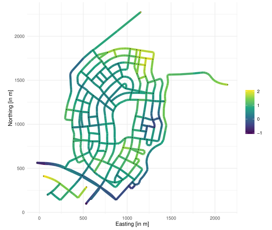
In the following simulation study, we consider the road network surrounding King Abdullah University of Science and Technology (KAUST), shown in Figure 3. The network geometry was retrieved using osmdata [22], which provides access to OpenStreetMap data, and was subsequently processed in QGIS. The resulting graph comprises 159 vertices and 263 edges. Its diameter, defined as the maximal shortest-path distance between any pair of vertices, is $4.8\text{\,}\mathrm{km}$. The graph is for demonstration of a real-world road system represented as a metric graph, that has a natural boundaries where the network is dense in a certain area, with many intersections close in space, and is connected to the rest of the network through longer edges. The graph was easily available from osmdata and used for demonstration in the MetricGraph vignette.

Two computational meshes are constructed on the network: (i) a coarse mesh with $m_{\tilde{h}}=165$ vertices and a maximum spacing of $\tilde{h}=$ 0.5 $\mathrm{km}$, and (ii) a fine mesh with $m_{h}=338$ vertices and a maximum spacing of $h=$ 0.1 $\mathrm{km}$. The coarse mesh contains six additional mesh vertices introduced along the longer edges, and locations are shown in Figure 3. Shorter edges do not require additional vertices as they are already below the defined maximum spacing. Similarly, the fine mesh contains 179 additional vertices introduced according to the same refinement procedure.

We consider $R$ independent replicates of the same GRF on the graph $\Gamma$,

where $4$ is the mean level and $u^{r}(\cdot)$ are independent samples from the same distribution induced by (2) under the chosen parameterization of $\rho(\cdot)$ and $\sigma(\cdot)$. For simplicity, we use the same observation locations for all replicates so that $\mathcal{S}^{r}=\mathcal{S}$, $\forall r$. As a consequence $N_{r}=N$, and the total number of observations is given by $n=N\cdot R$. Observation locations are sampled uniformly over the graph. Observations are defined by evaluating the replicates of $\eta(\cdot)$ in these locations and adding observation noise,

where the observation noise variance is set to $\sigma_{\mathrm{N}}^{2}=0.01^{2}$. Figure 4 shows one realization of the $\eta(\cdot)$ field in the non-stationary case and one example of the observation locations.

We consider two different scenarios for $u^{r}(\cdot)$. In the first scenario, $u^{r}(\cdot)$ is a stationary field with constant covariance parameters, $\log\rho(\boldsymbol{\mathbf{s}})=0.6$ and $\log\sigma(\boldsymbol{\mathbf{s}})=0.1$ for all $s\in\Gamma$. In the second scenario, $u^{r}(\cdot)$ is a non-stationary field whose range $\rho(\cdot)$ and standard deviation $\sigma(\cdot)$ vary over space. In this case, we simulate realizations of $\log\rho(\cdot)$ and $\log\sigma(\cdot)$ as independent WM-GRFs with approximate range 0.91 $\mathrm{km}$ and approximate standard deviation 0.92. Thus, using the interpretation from the one-dimensional SPDE approach, point-wise deviations from the mean are typically of order 0.92 on the log-scale and at distance 0.91 $\mathrm{km}$ the correlation is near 0.1. These parameters were chosen so that the covariance fields vary over the graph such that assumptions of WMF are too strict. The coarse mesh is used to sample the true covariance structure. Additionally, we add a constant to $\log\rho(\cdot)$ equal to $0.7$. We keep the resulting realizations fixed and the realizations of $\log\rho(\cdot)$ and $\log\sigma(\cdot)$ are shown in Figure 5.

We consider three values of $N$, corresponding to sparse ($N=50$), medium ($N=100$), and dense ($N=150$) spatial coverage. The levels were chosen to represent cases where one is close to having as many observations as we have vertices, and down to quite few observations compared to the number of vertices and edges. To illustrate three levels of temporal coverage, we consider three values of $R$, namely 5, 25, and 50. The levels are chosen with our application to modeling of traffic data in mind. If one consider a specific time window with traffic data, for example Monday 10:00-11:00am, each of the resolution levels correspond to approximately one month, six months and a year. For each of the 9 combinations of the resolution levels – simulation setting – we simulate 20 datasets that comes from randomly drawing observation locations from the simulated field, where each repeated experiment under the same simulation setting is independent of the next. For each dataset, we estimate the model parameters and predict the field $\eta(\boldsymbol{\mathbf{s}})$ in all vertices in $\mathcal{V}_{h}$.

For each of the two scenarios, we investigate how three models —namely, WMF, C-GWMF, and B-GWMF—perform as a function of the number $N$ of spatial observation locations and the number $R$ of temporal replicates. We next describe the specification of these three models in more detail.

All three models share the same hierarchical structure described in Section 3. For the mean component we let $\boldsymbol{\mathbf{\beta}}=[\beta_{0}]^{\mathrm{T}}$ and $\boldsymbol{\mathbf{X}}=\boldsymbol{\mathbf{1}}_{n}$, where $\boldsymbol{\mathbf{1}}_{n}$ is a $n\times 1$ vector of ones. Thus, the mean structure only consist of an intercept.

For the C-GWMF model, we create the covariate needed to model the covariance structure from the data as follows: At each observation location $\boldsymbol{\mathbf{s}}_{i}$, $i=1,\ldots,N$, we compute the empirical standard deviations of the observations $y^{r}(\boldsymbol{\mathbf{s}}_{i})$, $r=1,\ldots,\lfloor R/2\rfloor$, by

where $\bar{y}(\boldsymbol{\mathbf{s}}_{i})$ is the temporal average observed at station $\boldsymbol{\mathbf{s}}_{i}$, across replicates $r=1,\ldots,\lfloor R/2\rfloor$. Next, we create a continuous covariate by smoothing the log-transform of the empirical standard deviations, $\tilde{z}_{d}(\boldsymbol{\mathbf{s}}_{i})=\log(z_{d}(\boldsymbol{\mathbf{s}}_{i}))$, $i=1,\ldots,N$. We smooth using a model where $\boldsymbol{\mathbf{\tilde{z}}}_{d}=[\tilde{z}_{d}(\boldsymbol{\mathbf{s}}_{1}\>\ldots\>\tilde{z}_{d}(\boldsymbol{\mathbf{s}}_{N})]^{\mathrm{T}}$ are noisy observations of a WM-GRF, $\tilde{z}(\cdot)$ as follows

and $\tilde{z}(\cdot)$ can be described as the solution to the SPDE

We use the same mesh $\mathcal{V}_{h}$, and determine the precision matrix for weights $\boldsymbol{\mathbf{\tilde{z}}}=[\tilde{z}(v_{1})\>\ldots\>\tilde{z}(v_{m_{h}})]^{\mathrm{T}}$ and perform inference for the hierarchical model as described in the previous setting. The posterior mean is used as the covariate $\widehat{\tilde{z}}(\cdot)$ for both $\log\kappa(\cdot)$ and $\log\tau(\cdot)$ as was described in (6). Note that, when fitting this model, we use only the second half of the observations $y^{r}(\boldsymbol{\mathbf{s}}_{i})$ for $i=1,\ldots,N$ and $r=\lfloor R/2\rfloor+1,\ldots,R$, as the first half of the data cannot go twice into the model. That is, we get $\boldsymbol{\mathbf{Y}}=[{\boldsymbol{\mathbf{(}}y^{\lfloor R/2\rfloor+1}})^{\mathrm{T}}\>\ldots\>(\boldsymbol{\mathbf{y}}^{R})^{\mathrm{T}}]^{\mathrm{T}}$, and $n=N\cdot(R-\lfloor R/2\rfloor)$. The hierarchical model takes the form as we saw in (14) with $\boldsymbol{\mathbf{Q}}_{h,q}=\boldsymbol{\mathbf{Q}}_{h,2}$ and we only consider $\boldsymbol{\mathbf{w}}^{r}$, $r=\lfloor R/2\rfloor+1,\ldots,R$.

Choosing reasonable priors directly for $\kappa(\cdot)$ and $\tau(\cdot)$ is challenging, since these parameters do not have a direct physical interpretation. Instead, we recommend specifying prior information in terms of the approximate correlation range and marginal standard deviation using the transformations in (7). Prior means for $\rho(\cdot)$ and $\sigma(\cdot)$ can then be transformed to the corresponding values of $\kappa(\cdot)$ and $\tau(\cdot)$ on the log scale. In this parameterization, the regression coefficients associated with the covariate, $b_{2}^{\kappa}$ and $b_{2}^{\tau}$, naturally have prior mean zero, corresponding to no covariate effect. In the simulation study, the same prior is used for all simulated datasets and in both scenarios. The prior is specified using knowledge of the true covariance structure employed to generate the data and is not adapted to the individual datasets used for model fitting.

For both the WMF and B-GWMF model, the whole dataset is used for inference on model parameter. Therefore, $\boldsymbol{\mathbf{Y}}=[{\boldsymbol{\mathbf{y}}^{1}}^{\mathrm{T}}\>\ldots\>{\boldsymbol{\mathbf{y}}^{R}}^{\mathrm{T}}]^{\mathrm{T}}$ and $n=N\cdot R$, and the hierarchical model is as stated in (14).

The prior for $\boldsymbol{\mathbf{\theta}}$ in the simplest model WMF uses a domain-based prior for $\rho_{S}$. We set the median as 0.3 times the diameter of the bounding box of the graph. This gives a median of about 1$\mathrm{km}$ for $\rho_{S}$ (be aware that the priors are set for $\log\rho_{S}$). For $\sigma_{S}$ we choose a prior median of 1 (0 on log-scale). The precision is 0.1 for both $\log\kappa$ and $\log\tau$.

For B-GWMF, we use multivariate Gaussians with precision matrix as described in (11) with $\tau_{1}=0.01$ and $\tau_{2}=1$. We follow our suggested approach and consider different values of $\tau_{1}$ while $\tau_{2}=1$ is kept fixed, sample 100 times from $N(0,\boldsymbol{\mathbf{Q}}(\boldsymbol{\mathbf{\theta}})^{-1})$ and compute the 95%-quantiles across these samples. By visualizing the field and comparing these to the true covariance structure in Figure 5, we set $\tau_{1}=0.01$. Note that we use the same prior in both scenarios, including the spatially constant truth. In addition, we have a fixed offset parameter, $\log\rho_{0}$ (similar to $f_{0}$ in (9)), which we set as $0.5$, which is intentionally not equal to the true offset equal to 0.7. That is, we still have to rely on B-GWMF to correct the level of $\log\rho(\cdot)$ through the basis function weights $b^{\rho}_{j}$, $j=1,\ldots,m_{\tilde{h}}$.

We evaluate the models’ ability to recover the log-transformed range $\log\rho(\boldsymbol{\mathbf{s}})$ and log-transformed standard deviation $\log\sigma(\boldsymbol{\mathbf{s}})$ of the Whittle–Matérn fields $u^{r}(\boldsymbol{\mathbf{s}})$, $r=1,\ldots,R$ through root mean squared error (RMSE). Their ability to predict the field $\eta^{r}(\boldsymbol{\mathbf{s}})$, $r=1,\ldots,R$, at unobserved locations is evaluated with both RMSE and the continuous ranked probability score (CRPS). While the covariance parameter RMSE measures how well each model recovers the underlying covariance structure, the predictive scores quantify the quality of the latent field predictions regardless of whether the covariance parameters are recovered exactly. Since the data are simulated, both the true covariance fields and the latent fields are available, allowing all evaluation metrics to be computed directly. Differences between the estimated and true covariance structure at each mesh node of the coarser mesh $\mathcal{V}_{\tilde{h}}$ are assessed directly and RMSE is defined as:

where $f(\cdot)$ is either $\log\rho(\cdot)$ or $\log\sigma(\cdot)$. For WMF $\hat{f}(\cdot)$ is just a constant, while for C-GWMF we compute the transformations using (7). B-GWMF estimates the field directly on this scale.

We predict the latent field at each node of the finer mesh $\mathcal{V}_{h}$ and define the RMSE for the latent field as:

where $\hat{\eta}^{r}(\boldsymbol{\mathbf{s}}_{k})$ is the posterior mean of $\eta^{r}(\boldsymbol{\mathbf{s}}_{k})$. Similarly for CRPS, we compute

where $\text{sd}(\hat{\eta}^{r}(\boldsymbol{\mathbf{s}}_{k}))$ is the posterior standard deviation associated with the prediction $\hat{\eta}^{r}(\boldsymbol{\mathbf{s}}_{k})$, and

where $y$ is the observation, $\mu$ is the predicted value from the model and $\sigma$ is the model uncertainty.

We first present results for the WM-GRF scenario, where the true field has constant covariance parameters. In this case, the three models exhibit similar prediction performances for the latent field $\eta^{r}(\boldsymbol{\mathbf{s}})$, as measured by RMSE and CRPS when the number of replicates $R$ is equal or above 25, which is shown in Figure 10(a) and Figure 10(b). For the smallest number of replicates, however, B-GWMF performs somewhat worse than the two competing models. We note that B-GWMF uses the same prior specification in both simulation scenario considered. In practice, one could/should set a stricter prior when prior knowledge or exploratory analysis suggests that the covariance structure is (close to) spatially constant. Figures can be found in Appendix B.

When it comes to comparing the ability to recover the true covariance structure, WMF achieves the lowest RMSE across all simulation settings, with C-GWMF performing similarly, as can be seen in Figure 11(a) and Figure 11(b). For $R=50$, the models are consistently ranked, from best to worst with regards to RMSE for the covariance fields as WMF, C-GWMF and B-GWMF. This reflects the bias–variance trade-off: when the true covariance structure is spatially constant, the additional flexibility of C-GWMF and B-GWMF is unnecessary and can lead to the estimation of spurious spatial variation in the covariance parameters. Consequently, the simpler WMF model provides the most accurate recovery of the true covariance structure. Detailed results are provided in Appendix B.

We next consider results for the more challenging GWM-GRF scenario with covariance parameters vary in space as illustrated in Figure 5. We first consider the prediction of the field $\eta^{r}(\boldsymbol{\mathbf{s}})$. As expected, increasing the number of spatial observation locations $N$ reduces both the RMSE and CRPS for the two models that can estimate variation in the covariance structure (row-wise in Figure 6(a) and Figure 6(b)). Similarly, performance improves as the number of replicates increases. Overall, for $N\geq 100$ B-GWMF consistently provides the best predictive performance. When the number of both replicates ($R$) and spatial locations ($N$) is small, all models show similar performances, with a slight preference for B-GWMF. This is expected as, in this setting, the available data provide limited information about the spatially varying covariance structure, making it difficult for the more flexible models to exploit their additional degrees of freedom. When either $N$ or $R$ increases, the benefit of modeling spatially varying covariance parameters becomes increasingly apparent. This improvement is particularly evident in the CRPS results, where B-GWMF clearly outperforms the competing models already for (N=100).