Multi-strain epidemiological systems frequently exhibit self-sustained oscillations, yet severe algebraic complexity has long obstructed a complete analytical characterization of these dynamics. Seeking to bypass these barriers, we have identified a broad, analytically tractable class of two-strain models featuring asymmetric cross-immunity that precludes secondary infections for a single strain. This targeted structural simplification allows us to derive explicit expressions for coexistence equilibria and map their stability. We show that the relative transmission advantage of secondary infections fundamentally governs the onset of robust limit-cycle oscillations, extending previous narrow-borderline results. Crucially, numerical simulations reveal a rich macroscopic landscape where small-amplitude local oscillations coexist with large-amplitude, recurrent outbreak cycles. The structural robustness of these phenomena is confirmed by incorporating effects such as waning immunity and isolation and extending the framework beyond the analytically tractable class. These findings provide a clear mechanistic explanation for multi-strain epidemic cycles and offer a highly tractable baseline for future theoretical developments.
An Analytically Tractable Framework for Multi-Strain Epidemics: Resolving Algebraic Complexity to Map Oscillatory Dynamics
keywords
Multi-strain epidemic models, Bifurcation analysis , Partial cross-immunity , Analytical tractability , Self-sustained oscillations1 Introduction
Many infectious diseases, such as seasonal influenza and dengue fever, involve multiple co-circulating strains that interact dynamically through host immunity Martcheva 2015; Wormser and Pourbohloul 2008; Aguiar et al. 2022; Keeling and Rohani 2008. While the principle of competitive exclusion predicts that less fit strains should be driven to extinction, biological reality frequently defies this prediction. Instead, multi-strain systems frequently exhibit persistent coexistence and complex, self-sustained oscillations. Understanding the biological mechanisms that generate and sustain such oscillatory behavior is a fundamental issue in epidemiology, with important implications for forecasting epidemic trajectories and designing sustainable public health strategies.
A key candidate for driving these self-sustained oscillations is partial cross-immunity, an immunological interaction where prior infection with one strain confers incomplete protection against others. Mathematical models have shown that cross-immunity can generate a wide range of dynamical behaviors. Notably, models with additional structural complexity, such as age stratification, quarantine, or temporary cross-immunity tailored to specific pathogens, readily exhibit complex, self-sustained oscillations Gumel and Song 2008; Garba et al. 2013; Hussaini et al. 2016; Ferguson et al. 1999; Gupta et al. 1998; Nuño et al. 2005; Nuno et al. 2008; Thieme 2007; Kuddus et al. 2022; Castillo-Chavez et al. 1989; Kooi et al. 2014; Kooi et al. 2023; Kooi et al. 2013; Aguiar et al. 2011; Aguiar et al. 2013; Aguiar et al. 2008. In contrast, the foundational two-strain SIR framework with lifelong partial cross-immunity was initially found to produce only damped oscillations Andreasen et al. 1997; Castillo-Chavez et al. 1989; Nuño et al. 2005, and later work showed that sustained oscillations in this minimal model occur only under highly restrictive conditions Chung and Lui 2016.
Recently, Gavish Gavish 2026 identified a novel oscillatory regime within this minimal framework by demonstrating the failure of standard asymptotic expansions along a critical curve in parameter space. The modeling assumptions of that study, however, restricted the emergence of these oscillations to a case where one strain confers no cross-immunity to the other, while confining the oscillatory behavior to an extremely narrow parametric region. This specificity and narrowness raises two fundamental questions: are these newly discovered oscillations merely a mathematical artifact of a highly specific parameter set, or do they indicate a broader, biologically robust phenomenon? More generally, as noted in Chung and Lui 2016, the emergence of self-oscillations is “rather intriguing, as there seems to be no biological reasoning behind this phenomenon”. The biological rationale driving this behavior has remained elusive, leaving open a related question posed by Gavish 2026: what is biologically special about the newly identified curve of instability?
In this work, we address these questions and elucidate the biological drivers of self-sustained oscillations by systematically investigating a broad family of two-strain transmission models to map their oscillatory dynamics. However, a significant initial obstacle arises: in general models, the coexistence equilibrium is defined only implicitly as the solution to a complex nonlinear algebraic system, which makes extracting stability conditions analytically inaccessible. To overcome this barrier, we identify an analytically tractable subfamily of models that are still rich enough to sustain oscillatory phenomena. Specifically, we achieve this by deliberately precluding secondary infections for one strain. Although we employ this condition primarily as a theoretical tool to bypass algebraic complexity, such highly asymmetric cross-immunity dynamics map naturally to real-world interactions, such as the competitive exclusion observed between Bordetella pertussis and Bordetella parapertussis Wolfe et al. 2007. Establishing this structural frontier provides a clear analytical lens through which to map and study the system’s oscillatory behavior.
Utilizing this framework, we demonstrate that the onset of limit-cycle oscillations is governed by the overall relative transmission advantage of a secondary infection. We show how oscillations can emerge even when the two strains are completely symmetric, possessing identical epidemiological features. This finding provides critical context to the results in Gavish 2026. In retrospect, that study evaluated a borderline scenario residing precisely at the onset of instability, explaining why the previously identified oscillatory regime was so parametrically narrow. By relaxing these restrictive historical assumptions and moving away from this mathematical borderline, we uncover parameter regions that support far more robust oscillations.
From an epidemiological perspective, focusing on a family of models that precludes secondary infections for one strain may appear restrictive, given that bidirectional secondary infections are common in many multi-strain systems. However, this specific framework allows us to explicitly incorporate complex biological and behavioral features, such as Antibody-Dependent Enhancement (ADE), waning immunity, and isolation, without rendering the mathematical stability analysis intractable. To demonstrate the utility of this approach, we analyze an extended system incorporating both waning immunity and isolation. We observe that, despite a significantly faster timescale for susceptible replenishment driven by waning immunity, the system preserves the same characteristic oscillatory patterns as the base model. Finally, to test the potential breadth of these findings without exceeding the scope of the current work, we conduct an initial numerical exploration of systems where secondary infections are permitted for both strains, as is typical for influenza Andreasen et al. 1997. We observe that the oscillatory dynamics extend to these broader cases, strongly suggesting that the fundamental instability mechanism identified here is structurally robust.
While our study investigates oscillatory dynamics predominantly through the lens of the coexistence equilibrium and its local stability, conforming with standard approaches in mathematical epidemiology, we identified a second, distinct oscillatory mechanism in multiple case studies. This unexpected phenomenon is characterized by large-amplitude recurrent outbreaks. We provide clear numerical observations of these macroscopic cycles and demonstrate that they can coexist with small-amplitude local oscillations. Characterizing the boundaries of these global transitions remains a compelling open problem. Although a full investigation of these global dynamics falls outside the scope of the present work, we use the discussion section to outline the separate global mechanism driving these macroscopic cycles, thereby establishing a foundational scaffold for a companion paper dedicated to characterizing this global phenomenon.
This paper is organized as follows. In Section 2, we introduce the criteria for selecting our analytically tractable family of two-strain models and present the specific base model. Section 3 provides explicit expressions for the single-strain and coexistence equilibria. In Section 4, we investigate the stability of the coexistence steady state employing a perturbation analysis to identify the parameter regimes that lead to oscillatory instabilities. We complement this analysis with a numerical study in Section 5 to explore the different types of oscillatory solutions that emerge. The robustness of these findings is evaluated in Section 6, which considers an extended model incorporating waning immunity and quarantine measures, and in Section 7, which considers models beyond the analytically tractable family of models. Finally, Section 8 provides a summary and discussion of our implications, highlighting the global oscillatory mechanisms to be explored in a companion paper.
1.1 Two-Strain Transmission Base Model
We consider, as a basis, the standard two-strain transmission model for the dynamics of partial cross-immunity, where infection by one strain may provide reduced susceptibility to infection by the other Castillo-Chavez et al. 1989; Martcheva 2015; Thieme 2007. Significantly, we extend this base model by allowing the recovery time from secondary infections to differ from the recovery time from primary infections.
As shown in Figure 1, we assume the population mixes randomly and is divided into eight relative compartments: Susceptibles (); individuals infected with a primary infection of strain (); individuals recovered from a primary infection with strain (); individuals infected with strain after having recovered from strain (, secondary infection); and individuals recovered from both strains (). The model is given by the following system of equations:
| (1a) | ||||
| (1b) | ||||
| (1c) | ||||
| (1d) | ||||
| (1e) | ||||
| (1f) | ||||
| (1g) | ||||
where is the birth and mortality rate, is the transmission coefficient for strain , is the recovery rate from strain , and is the recovery rate from a secondary infection with strain . Additionally, is the relative susceptibility to strain for an individual previously infected and recovered from strain (), where corresponds to reduced susceptibility (partial cross-immunity), corresponds to neutral susceptibility (no cross-immunity) and corresponds to enhanced susceptibility. The relative infectivity of individuals with a secondary infection of strain , compared to those with a primary infection, is denoted by .
2 Model Selection: Criteria and Identification
We wish to identify a family of analytically tractable models suitable for studying oscillatory phenomena. We begin by listing the primary criteria for determining such a family of two-strain models:
- 1.
Asymmetry Between Strains: Symmetric models are commonly studied because they are mathematically tractable Chung and Lui 2016; Castillo-Chavez et al. 1989, yet they may not accurately represent real-world epidemiological dynamics where strains exhibit distinct biological profiles Aguiar et al. 2011; Kooi et al. 2014. Even introducing weak asymmetry can reveal novel phenomena that purely symmetric models overlook, as demonstrated by the narrow oscillatory regime recently identified in Gavish 2026. Therefore, we seek asymmetric models with the belief that they are likely to provide a clearer, more robust framework to capture and analyze the generic oscillatory phenomena driven by these biological imbalances.
- 2.
Explicit Expression for the Coexistence Steady-State: The endemic steady-state of coexistence is the solution to a nonlinear algebraic system. While numerical studies have long shown limit cycles in asymmetric models, the algebraic complexity of this equilibrium has historically precluded the derivation of explicit, analytical criteria for the onset of these oscillations. Implicit or cumbersome expressions for the steady-state variables significantly complicate stability analysis or make it intractable Chung and Lui 2016; Castillo-Chavez et al. 1989; Martcheva 2015; Gavish 2026. Finding a family of models characterized by an explicit and simple coexistence steady-state is a technical necessity to unlock the algebraic thresholds governing these oscillations.
- 3.
Broad Family of Models: To gain insight from multiple models, we require a broad family of models that satisfies the above two requirements, rather than a single carefully selected model.
To meet these objectives, a delicate mathematical balance must be struck. While satisfying all three criteria simultaneously poses a challenge, we demonstrate that preventing secondary infections with one strain provides a straightforward mathematical scalpel to achieve this. Let us consider model (1) with . Requirement 1 is met because the model is inherently asymmetric, allowing secondary infections only with strain 2. Requirement 2 is also satisfied, as the coexistence steady-state becomes defined by a clear and straightforward expression. By definition, when secondary infections with strain 1 are impossible. As a result, Equation (1b) simplifies to
leading to a simple expression for at equilibrium:
Substitution of the above value for removes nonlinear terms such as from the algebraic equations describing the coexistence steady-state, allowing one to explicitly solve the remaining linear system, as detailed in Section 3. Finally, the assumption that eliminates secondary infections for one strain can be applied across a broad family of two-strain models. For example, in Section 6, we find explicit expressions for the coexistence steady-state in an extended two-strain model with quarantine and waning immunity. Thus, requirement 3 is also satisfied.
Although mathematical necessity narrowed our focus from the general two-strain case to this specific model family, we emphasize that this choice is primarily an analytical tool. It is well established that general two-strain models can exhibit complex dynamics, including Hopf bifurcations and chaos, even without external forcing Aguiar et al. 2008; Aguiar et al. 2011; Kooi et al. 2013. Therefore, precluding secondary infections for one strain () is not introduced to claim structural novelty, but rather to explicitly bypass the severe algebraic complexity that typically obscures the coexistence equilibrium. Nevertheless, this structural simplification remains firmly rooted in biological reality. Strongly asymmetric cross-immunity dynamics have been documented in real-world pathogen interactions, such as the competitive exclusion observed between Bordetella pertussis and Bordetella parapertussis Wolfe et al. 2007. Ultimately, this overarching methodological strategy, deriving a specific, analytically tractable model family from objective criteria to illuminate macroscopic behaviors, proves highly effective here. As subsequent sections will demonstrate, this targeted approach successfully extracts the robust analytical mechanisms that drive epidemic cycles.
2.1 Model of Study
Having established the utility of a model family where secondary infections with one strain are excluded, we now define the specific model for our study. For brevity, we derive this by substituting into the general model (1) and aggregating the compartments and into a single compartment .

The disease dynamics for this reduced model are schematically depicted in Figure 2 and governed by the following system:
| (2a) | ||||
| (2b) | ||||
| (2c) | ||||
| (2d) | ||||
| (2e) | ||||
| (2f) | ||||
We consider initial conditions that satisfy
| (3) |
which ensures that for all ,
| (4) |
In what follows, we use the algebraic relation (4) to express in terms of the other compartment sizes and consider the model as a system of the remaining equations (2a)–(2e). We consider the model (2) with vital dynamics , restricting the feasible parameter space to strictly positive values:
| (5) |
A standard computation of the basic reproduction number, e.g., as in Chung and Lui 2016; Castillo-Chavez et al. 1989, yields
where
| (6) |
3 Steady States
The system (2) has a disease-free equilibrium, , that is stable, by definition, when , and two single-strain endemic states for :
- 1.
If , there exists a steady-state of (2) with compartment sizes
(7) - 2.
If , then there exists a steady-state of (2) with compartment sizes
(8)
The invasion numbers, , of strain at the endemic equilibrium, , of strain (for and ) are computed as in (Martcheva 2015, Ch. 8.4):
| (9) |
In accordance with standard epidemiological theory, the endemic steady state is linearly stable if and only if the invasion reproduction number of the competing strain is strictly less than one.
Proposition 1 (Stability of Single-Strain Steady States).
Let such that the single-strain endemic steady state, , of system (2) exists. Then, is linearly stable if and only if the invasion number, , of the competing strain is strictly less than one:
Proof.
We, therefore, obtain a partition of the plane into several domains based on the stability of the disease-free and single-strain equilibria, as illustrated in Figure 3:
| (10) |
where (gray region) is the domain in which the disease-free equilibrium is stable, and (blue region) and (red region) are the domains where the single-strain endemic states and are stable, respectively.
The following proposition shows the existence of a unique steady-state of coexistence in the complementary regime (green region), defined as:
| (11) |
Proposition 2 (Coexistence Steady State).
Let . Then, system (2) possesses a unique coexistence steady state, , characterized by strictly positive infectious populations and . The compartment sizes of are given by:
| (12a) | |||
| where | |||
| (12b) | |||
4 Stability of the Coexistence Steady State
Direct stability analysis of via the Routh-Hurwitz criteria is intractable due to the complexity of the quintic characteristic polynomial. To address this, we follow established methodologies in the literature Andreasen et al. 1997; Dawes and Gog 2002; Chung and Lui 2016; Gavish 2026 and analyze the system in the asymptotic regime
| (13) |
which corresponds to a demographic turnover rate significantly slower than the disease recovery rates. This separation of time scales is characteristic of acute infections like influenza or dengue, where the infectious period (days/weeks) is negligible compared to the host lifespan (decades) Nemhauser et al. 2023. Mathematically, this represents a singular perturbation problem, as the coexistence equilibrium vanishes in the limit .
Building on this framework, we apply the singular perturbation approach utilized in Gavish 2026. In that study, the method was applied to a model with mutual partial cross-immunity () under the restricted assumptions of symmetric parameters for secondary infections: identical recovery rates () and equal infectivity (). Consequently, that analysis pointed to instability in a rather limited region, specifically when either or . Here, we apply the same mathematical approach to the strongly asymmetric model (), but we allow for general positive secondary epidemiological parameters ( and ). Significantly, this generalization yields vastly different outcomes, uncovering a much broader instability regime that reduces previous work to a borderline case.
The characteristic polynomial of the Jacobian of (2) at takes the form
| (14) |
where
| (15) |
where is the degree of each polynomial . The coefficients, , depend on the parameters of the problem. The explicit expressions for are available through symbolic computation and are generally long and cumbersome. For conciseness, we will provide explicit expressions only for the coefficients whose form and dependence on parameters are used in the stability analysis.
The polynomial has five roots. Four roots are of order ,
| (16a) | |||
| where are the roots of | |||
| (16b) | |||
and an additional root that satisfies
The latter root is negative in the feasible parameter space, i.e., when .
We now consider the roots (16). To simplify the stability criteria, we group the parameters into constants and defined as
| (17) |
so that the coefficients of (16b) read as
For , and . Thus, and . The discriminant, , of the quadratic equation (16b) equals
where
and
| (18) |
The analysis gives rise to a new quantity, .
Biologically, quantifies the relative transmission advantage of secondary infections. This advantage can stem from heightened infectivity (), decreased crossed-immunity or enhanced susceptibility (), or a longer infectious period (). Crucially, this formulation reveals that instability does not strictly require weak cross-immunity () as Gavish 2026 implied. Rather, instability emerges whenever the combined epidemiological traits of a secondary infection confer an overall transmission advantage ().
Remark 1.
The invasion number , see (9), equals
| (19) |
so that the ratio relates to the contribution of secondary infections to the invasion number.
In the case , it follows that , and hence for . This implies that the relevant eigenvalues are purely imaginary at leading order, and stability is determined by the next-order terms. Numerous works, e.g., Andreasen et al. 1997; Gomes and Medley 2002; Dawes and Gog 2002; Chung and Lui 2016, have derived these terms, revealing long and cumbersome expressions from which stability could only be determined in highly specific parameter cases. We will not pursue this direction here but will present numerical results suggesting that the coexistence steady-state is stable in this parameter regime.
When , the second term of is negative, and therefore can become negative if is sufficiently close to . The following lemma points to a single curve in the parameter space along which .
Lemma 1.
Proof.
See Appendix 10. ∎
Following Lemma 1, if , then along . In this case, at least one of the roots has a positive real part, and therefore the coexistence steady-state is unstable along .
In the borderline case, , only when . Here, stability is determined by the next-order terms. Expressions (17) for and reduce to
so that
Following Gavish 2026, to ascertain stability when , we consider the higher-order expansion
| (20) |
Substituting (20) into and equating powers of yields, at leading order,
At the next order, we have
| (21) |
Given , the subsequent order yields
| (22) |
Note that is purely imaginary. Consequently,
Hence, two of the eigenvalues have a positive real part, and thus the coexistence steady-state is unstable along and in its vicinity.
The following Proposition summarizes the analytical results attained in this section.
Proposition 3 (Instability along ).
Remark 2.
The analysis in Gavish 2026 examines the stability of with respect to the dynamics of the more general model (1) in the regime . In retrospect, the restrictive assumptions of that study caused condition (23) to simplify to , meaning the analysis was effectively constrained to identifying instability only in the mathematical borderline case with . Consequently, the current analysis serves as an analytical refinement and generalization of Gavish 2026. By relaxing the prior restricted assumptions, we demonstrate that the previously identified instability is not merely an isolated consequence of a mathematical borderline, but rather a specific instance of a much broader and biologically robust oscillatory regime. Furthermore, the fact that the condition remains applicable in Gavish 2026 for any , rather than being restricted to the limit , suggests that the current analysis extends beyond the base model (2). See also Section 7.
5 Numerical Study
The analysis in Section 4 shows that when secondary infections possess a relative transmission advantage over primary infections, , there exists a parameter region in which the coexistence steady-state, , is unstable, and that this region includes the curve . However, the analysis does not address the dynamics of beyond this characterized region. Therefore, it is not clear whether the steady state is stable outside this regime or if other regions of instability exist. Furthermore, our analytical results do not provide information on the global dynamics of the system when is unstable, for example, whether its solutions converge to a periodic limit cycle or display more complicated dynamics. In this section, we complement the analysis with a numerical study to obtain a clearer picture of the system’s global behavior. Numerical details are provided in Appendix 11.

Figure 4 presents a bifurcation diagram for the base model (2) across several values of , the relative transmission advantage of a secondary infection. In all cases, we set and ; thus, assuming a time unit of one week, the average recovery time from a primary infection with strain 1 is one week, and the mean host lifespan is roughly 76 years. While Proposition 3 formally establishes instability for sufficiently small , this parameter choice acts to confirm that the predicted oscillatory behavior robustly arises under biologically realistic values of and .
To construct this scenario, we choose parameters that confer a slight transmission advantage to secondary infections: heightened infectivity () and enhanced susceptibility (). However, the overall transmission advantage, , is ultimately determined by the duration of the secondary infectious period, . For our chosen values, setting yields secondary recovery rates of and , respectively, corresponding to recovery periods of days. Furthermore, exploring other parameter combinations, such as neutral infectivity () and partial cross-immunity (), produces no qualitative change in the system’s dynamics, see Appendix 12.
Figure 4I shows the case , where the secondary transmission advantage satisfies condition (23). Within the coexistence region , the steady state is computed and its linear stability is evaluated via the spectral radius of the corresponding Jacobian, , with stable regimes colored blue and unstable regimes colored red. As Proposition 3 implies, a distinct region of instability (red) emerges, with the critical curve (black dotted curve) lying safely within its interior.
Figure 4III presents the case , for which condition (23) is not satisfied. We observe that is stable whenever it exists, providing numerical evidence that the next-order terms maintain the stability of the coexistence equilibrium in this regime. Finally, Figure 4II shows the borderline case . In accordance with Proposition 3, we observe that is unstable in a narrow regime the vicinity of the curve .

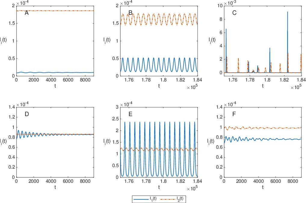
To visualize the system’s dynamics across different parameter regimes, Figures 5A-F present the temporal solutions of (2) corresponding to points A-F in Figure 4, all initialized near coexistence (). Points A, D, and F reside in the stability region of ; as expected, the corresponding solutions naturally converge to this steady state (Figures 5A, 5D, and 5F, respectively). Conversely, when is unstable, all steady states of the bounded system are unstable, precluding convergence to an equilibrium and resulting in sustained oscillatory or complex dynamics. Points B and E lie near the boundary of this instability region (Figures 4I and 4II, respectively). We observe that the solutions exhibit small-amplitude oscillations centered around , consistent with the local Hopf-like findings of previous research Chung and Lui 2016; Gavish 2026. Surprisingly, at point C, located well within the instability region, we observe a drastically distinct dynamic. The solution consists of short, intense surges of strain 1, followed by a surge of strain 2, and a subsequent low-prevalence time interval before a new cycle begins. The numerical investigation in the next subsection will focus on these unexpected oscillations, and show that they can coexist with the small-amplitude Hopf-like limit cycles.
The parameters chosen for the graphs in this section correspond to heightened infectivity and enhanced susceptibility ( and ) of secondary infections compared to a primary infection, whereas the overall relative transmission advantage or disadvantage of a secondary infection over a primary infection, , determines the duration of the infectious period, . To demonstrate that the key parameter determining the stability behavior of is , rather than the parameters that it depends on, we present in Appendix 12 an additional numerical example with parameters that reflect neutral infectivity and partial cross-immunity ( and ). As expected, the qualitative results are the same.
5.1 Observation of an additional oscillatory mechanism
The oscillatory solution in Figure 5B exhibits a small-amplitude oscillation, whereas the solution in Figure 5C demonstrates large-amplitude, outbreak-like behavior. To establish whether these distinct behaviors stem from coexisting attractors at the exact same parameter choices, we investigate the system’s sensitivity to initial conditions. Figure 6 demonstrates a striking bistability for the parameters corresponding to point B in Figure 4I (). When initialized in close proximity to the coexistence equilibrium via a minor perturbation, explicitly constructed by setting and scale-normalizing the remaining compartments to preserve the unit population invariant , see (24), the trajectory approaches a low-amplitude limit cycle enclosing (Figure 6A, and the red dash-dotted curve in Figure 6C). Conversely, under the identical parameter set, initiating the system near the single-strain equilibrium by introducing a trace invader population (with the remaining non-zero compartments of scale-normalized accordingly) uncovers a distinct, large-amplitude oscillatory attractor (Figure 6B, and the gray curve in Figure 6C). Numerical continuation shows that this bistability persists under small parameter perturbations and is not a fine-tuned numerical artifact. As discussed in Section 8, in a companion paper, we will demonstrate that this distinct, large-amplitude oscillatory mechanism is driven by a Shilnikov-like orbit connected to a single-strain equilibrium.

To systematically map how these different oscillatory behaviors are distributed across the parameter space, we monitor the spike amplitude for solutions of (2) along the line where the initial condition is near , specifically we take
| (24) |
while the rest of the variables remain the same as , up to normalization, .

The region of instability of is marked by a shaded gray area in Figure 7A. As expected, in this region, we observe that the solution is oscillatory. We observe that the system exhibits small-amplitude oscillations near the boundaries, see inset graphs in Figure 7 for a zoom-in on the boundaries of the instability region. For instance, Figure 7B provides an example of this behavior near the lower boundary of the instability region (), while Figure 7G illustrates a similar small-amplitude pattern near the upper boundary (). However, the one-parameter bifurcation diagram in Figure 7A reveals that, for the above initial conditions, these Hopf-like limit cycles do not extend to the full instability region. Throughout the vast majority of the instability region’s interior, the system solutions transition into large-amplitude, outbreak-like oscillations, see Figures 7C-F. Particularly, within the region of large-amplitude oscillations, we observe two sub-regions, and , where the solution peaks reach a unique value. These regions correspond to regular and periodic large-amplitude oscillations, as observed in Figures 7D and 7F. The complementary regions correspond to more complex oscillatory patterns, possibly aperiodic, as observed in Figures 7C and E.
6 Analytical Tractability and Structural Robustness within the Family
The overarching goal of this study is to better understand oscillatory phenomena in multi-strain epidemic systems through an analytically tractable family of models. To demonstrate this tractability, we show that the coexistence equilibrium, , can be explicitly computed even for a highly complex generalization of the baseline model. Analyzing this extended formulation also allows us to establish the structural robustness of our primary results. Specifically, by incorporating realistic epidemiological conditions, such as waning immunity and the isolation of primarily infected individuals, we confirm that the analytically derived instability regime and oscillatory behavior persist well beyond the base formulation. The subsequent section demonstrates that this structural robustness extends even to models outside the family.
In the following we consider an extended model with waning immunity that includes two additional isolation compartments, , for those infected with strain . To distinguish between recovery histories, we also introduce a compartment for individuals recovered from a primary infection with strain 2, while reserving compartment exclusively for those recovered from a secondary infection. The schematic diagram of this extended model is shown in Figure 8.

The extended model is given by the following system of equations:
| (25a) | ||||
| (25b) | ||||
| (25c) | ||||
| (25d) | ||||
| (25e) | ||||
| (25f) | ||||
| (25g) | ||||
| (25h) | ||||
| (25i) | ||||
where is the rate at which individuals infected with strain are isolated, and is the rate at which they recover and are released from isolation. The rate at which immunity wanes following a primary infection with strain is denoted by , and the waning rate after a secondary infection is denoted by . Note that when , the dynamics of those recovered from an infection with strain 2 are independent of whether it was a primary or secondary infection; in such cases, the compartments and can be combined, reducing to a structure closer to that of model (2).
Similar to the base model, we consider non-negative initial compartment sizes that sum to one. For the extended model parameters, we require the following conditions:
| (26) |
in addition to the baseline feasible space defined in (5). The basic reproduction number of (25) reads as
where the strain-specific reproduction numbers are now updated to account for isolation:
| (27) |
6.1 Analytic tractability
Similar to the base model, we begin by establishing the single-strain endemic equilibria. If , system (25) admits a single-strain steady state . The compartment sizes of are:
| (28) |
and the compartment sizes of are:
| (29) |
To determine the stability of these boundary steady states and the conditions for coexistence, we define the invasion reproduction numbers for the extended model. The invasion number of strain 2 into the endemic equilibrium of strain 1 is given by:
| (30) |
Conversely, because strain 2 does not generate secondary infections by strain 1 (), the invasion number of strain 1 into the endemic equilibrium of strain 2 reduces simply to:
| (31) |
Using these invasion numbers, we define the extended coexistence region, , as the parameter space where both strains can mutually invade:
| (32) |
With the steady states and invasion boundaries established, the stability and coexistence conditions follow directly:
Proposition 4 (Stability of Single-Strain Steady States).
Let such that the single-strain endemic steady state , of system (25) exists. Then, is linearly stable if and only if the invasion number, , of the competing strain is stricly less than one:
Proof.
See Appendix 9. ∎
Proposition 5 (Coexistence Steady State).
Let . Then, system (25) possesses a unique coexistence steady state, , characterized by strictly positive infectious populations and . The compartment sizes of are given by:
| (33a) | |||
| where | |||
| (33b) | |||
Proof.
See Appendix 13. ∎
Proposition 5 demonstrates how the core assumption, the elimination of secondary infections by strain 1 (), preserves the mathematical tractability of the model by yielding an explicit expression for the coexistence steady state even in a highly complex model featuring quarantine and waning immunity.
6.2 Structural robustness
The extended model (25) differs from the base formulation by incorporating two distinct mechanisms for susceptible replenishment: a slow demographic turnover, as in the base model, and a significantly faster mechanism driven by the waning of immunity. This addition alters the asymptotic structure underpinning the analytical results in Section 4. Consequently, it is not a priori clear whether the extended model will preserve the oscillatory dynamics of the base system. While a full mathematical analysis of this extended case is beyond the scope of the current paper, we present a numerical analysis demonstrating that the system’s dynamics exhibit remarkable structural robustness. To evaluate this robustness, we consider the extended model under a biologically plausible parameter set:
| (34) |
Assuming a time unit of one week, this configuration represents realistic recovery and isolation periods of approximately one week, alongside immunity waning over a timescale of roughly two years. These values also reflect slight, realistic asymmetries between the two strains. As in the numerical example of Figure 4, we determine according to the value of the relative transmission advantage.
In the base model (2), the analysis identified the parameter as the exact relative transmission advantage determining the onset of limit-cycle instabilities. Lacking a closed-form transcendental expression for the exact bifurcation threshold in the higher-dimensional framework, we introduce a structural analogue, , to serve as an interpretive heuristic and parameter-scaling tool. This heuristic leverages the property that the threshold scales with the ratio of secondary to primary infectious period durations weighted by susceptibility and infectivity adjustments. Transposing this relation to the extended framework with quarantine, we define:
| (35) |
We emphasize that is not used as an approximate classification metric for our stability boundaries. Because Proposition 5 yields an explicit expression for the coexistence steady state , the linear stability of the system is evaluated exactly and directly by computing the eigenvalues of the full Jacobian matrix across our parameter sweeps. Instead, we employ (35) as a scaling rule to explicitly isolate and calibrate the secondary recovery rate:
| (36) |
This allows us to evaluate the structural robustness of the instability mechanism under comparable transmission conditions across different versions of the model.

Figure 9I presents the bifurcation diagram in the plane for . As expected, we observe a substantial oscillatory region, resembling Figure 4I. Within this region, we mark two distinct points, A and B, which are dynamically analogous to points B and C in the base model (Figure 4), respectively. As in the base model, point A exhibits a local periodic limit cycle about , see Figure 10A, while point B gives rise to larger-amplitude outbreaks interspersed with low-activity periods, see Figure 10B.

However, the dynamical differences between the small-amplitude (point A) and large-amplitude (point B) oscillations are significantly less pronounced in the extended model. The amplitude ratio between these two solutions is approximately 3, a stark contrast to the ratio of roughly 200 observed between the analogous solutions in the base model. Moreover, the extended model exhibits much shorter low-activity periods, which are comparable in length to the duration of the high-activity outbreaks. Furthermore, bifurcation analysis reveals that the oscillatory solutions of the extended model remain entirely regular, see Figure 11, whereas the base model exhibited both regular and irregular oscillations, see Figure 7. It is highly plausible that the faster replenishment of susceptible in the extended model acts to dampen extreme fluctuations, thereby contributing to these observed changes in amplitude scaling, temporal clustering, and regularity.

Figure 9II presents the exact numerical bifurcation diagram evaluated for . We observe that this choice represents a borderline scenario, dynamically analogous to the base model threshold behavior shown in Figure 4II. Conversely, when setting (Figure 9III), the unstable oscillatory region is completely absent from the feasible parameter space.
Based on these exact numerical stability computations, we find that for the chosen parameter configuration (34), the transition to instability occurs at an empirical threshold value satisfying . This conditional observation confirms that while functions as a reliable and highly accurate heuristic for scaling parameters and identifying the structural conditions that spark instabilities, the fast susceptible replenishment introduced by waning immunity slightly shifts the true analytical boundary away from unity.
In summary, despite the differences between the base model and the extended model, both share key structural features regarding their oscillatory behavior. Specifically, both frameworks capture the emergence of oscillations beyond the critical threshold quantity and demonstrate distinct regimes of low-amplitude versus high-amplitude oscillations. Crucially, the explicit availability of the coexistence steady-state , see Proposition 5, establishes a pathway for subsequent analytic studies. While further research is necessary to refine our understanding of the complex impact of waning immunity, the foundational approach taken in this work has proven highly fruitful, yielding critical insights into the underlying mechanisms that drive epidemic cycles.
7 An outlook on Structural Robustness Beyond the Family
This work aims to better understand oscillatory phenomena in multi-strain epidemic systems by focusing on an analytically tractable family of models where secondary infections with one strain are excluded (). This approach proved highly successful, revealing the critical role of , the curve, and the limiting case in which the oscillatory domain is confined to the vicinity of . Furthermore, pinpointing the domain where small-amplitude oscillations arise enables the identification of additional oscillatory mechanisms and provides clear directions for future research. To test the potential breadth of these findings without exceeding the scope of the current work, we conduct an initial numerical exploration to determine whether these dynamics extend to cases where .
Figure 12 presents bifurcation diagrams for model (1) as a function of and across three distinct cases. Because this model allows for secondary infections from both strains, we define as the analogue to (18). This parameter represents the relative transmission advantage of a secondary infection with strain one over a primary infection with strain two:
When , the coexistence equilibrium is no longer available in a fully decoupled closed-form vector like in the specialized family. However, the steady-state equations can still be reduced exactly to a cubic polynomial in terms of the susceptible population Gavish 2026. At each parameter coordinate, the roots of this cubic polynomial are computed algebraically using standard matrix companion methods via MATLAB’s roots routine. Feasibility and uniqueness are strictly enforced by filtering for a real root that lies within the domain . Once this unique value of is established, the remaining epidemiological compartments are evaluated sequentially via explicit closed-form algebraic expressions of .
The first case explores the dynamics of cocirculating strains driven by partial, symmetric cross-immunity (). Such a scenario holds strong biological relevance and has been used to model diseases such as influenza, see, e.g., Andreasen et al. 1997. Here, primary infections maintain a relative transmission advantage over secondary infections, analogous to the scenario presented in Figure 4A. As expected, we observe that the coexistence steady-state is stable whenever it exists, see Figure 12A.
The second case explores an asymmetric scenario where only secondary infections with strain one possess a relative transmission advantage over primary infections with strain two (). Similar to the case in Figure 4B where and , we observe a parameter region where becomes unstable, indicated by the red region in Figure 12B. To systematically map the distribution of oscillatory behaviors across the parameter space, we monitor the spike amplitudes for solutions of model (1) along the line , where the initial condition is near , see Figure 13A. Resembling the approach and dynamics of Figure 7A, the system exhibits regions of low-amplitude oscillations (e.g., Figures 13B–D), as well as both regular and irregular high-amplitude oscillations (Figures 13E and 13F).
Finally, we consider dynamics induced by antibody-dependent enhancement (ADE), following the framework of Ferguson et al. Ferguson et al. 1999. In this case, secondary infections hold a relative transmission advantage over primary infections. Crucially, while this case includes symmetric strain parameters, the system still exhibits robust oscillatory dynamics (see the red region in Figure 12C). This demonstrates that these oscillations are fundamentally driven by the relative advantage of secondary infections rather than parametric asymmetry. Indeed, the bifurcation diagram reveals that the oscillatory region spans a segment of the line, where the two strains are completely symmetric. However, unlike all other cases considered in this work, this oscillatory region lies strictly along the boundary of the existence region for . Evaluating the corresponding spike amplitudes (Figure 14A), we observe a continued diversity in the oscillatory regimes: regular and irregular high-amplitude solutions (Figures 14B–D), alongside distinct low-amplitude oscillations (Figures 14E–G). It is important to contextualize these findings relative to diseases like dengue fever. While ADE is notably linked to dengue fever Ferguson et al. 1999, model (1) does not capture the more intricate immunological complexities, such as temporary cross-immunity, associated with the disease Aguiar et al. 2022.


Ultimately, exploring parameter regimes where reveals that the core oscillatory phenomena identified in our analytically tractable base model are highly robust. Even though the coexistence steady-state is no longer explicitly solvable in this extended setting, numerical investigations confirm the persistence of key structural features: the threshold-driven onset of oscillations and the clear bifurcation into low- and high-amplitude regimes. Although further research is necessary to fully unravel the complex interactions in these extended regimes, the foundational approach taken in this work has proven highly fruitful. By analyzing the tractable base model, we have established a robust framework that yields critical insights into the underlying mechanisms driving multi-strain epidemic cycles.
8 Discussion
This study introduces a family of analytically tractable two-strain models defined by the parameter choice . This restriction bypasses the algebraic complexity typically associated with the coexistence equilibrium, enabling a rigorous analysis of oscillatory phenomena even when incorporating features like antibody-dependent enhancement (ADE) () and asymmetric recovery rates. This approach showed that the relative transmission advantage of a secondary infection is the primary driver of limit-cycle oscillations. The results provide new context to the results in Gavish 2026. In retrospect, that study evaluated a borderline scenario residing precisely at the onset of instability, explaining why the previously identified oscillatory regime was so parametrically narrow. Moving away from this mathematical borderline, we uncover parameter regions that support far more robust oscillations, dynamic behaviors that likely better reflect real biological conditions.
While mapping these small-amplitude oscillations, we encountered an unexpected phenomenon: the emergence of distinct, large-amplitude outbreak cycles, even when the initial condition is near the coexistence equilibrium. These macroscopic oscillations operate independently of the local Hopf bifurcation. Under certain initial conditions, they dominate the phase space, generating a bistability where a stable steady state coexists with a massive oscillatory attractor. From a dynamical systems perspective, this transition points to a rich topological complexity likely involving global bifurcations—potentially homoclinic or Shilnikov-like—associated with saddle-focus equilibria. Characterizing the boundaries of these global transitions remains a compelling open problem. Our mathematically transparent baseline provides an ideal scaffold for mapping these complex global dynamics and extending methods used to chart multi-strain structures Aguiar et al. 2015.
Our numerical investigations (Sections 6 and 7) strongly suggest that the fundamental instability mechanisms driving limit-cycle oscillations and high-amplitude outbreaks are structurally robust. Oscillations persist when incorporating temporary cross-immunity (waning immunity), quarantine measures, or secondary infections from both strains. While our exploration is not exhaustive, it leaves the characterization of their complete dynamical landscape for future work.
The framework developed here may provide a theoretical basis for further mathematical investigation of multi-strain dynamics in epidemiological systems. The core assumption of precluding secondary infections for one strain () maps naturally to the strongly asymmetric cross-immunity observed between Bordetella pertussis and Bordetella parapertussis Wolfe et al. 2007. Permitting secondary infections for both strains (), as shown in Figure 12B, provides a baseline for studying antigenically drifting respiratory pathogens like influenza, where bidirectional partial cross-immunity shapes epidemic cycles Andreasen et al. 1997. The framework also accommodates targeted extensions for ADE and temporary waning immunity (Figures 9 and 12C). While both features are classically linked to the macroscopic cycles of dengue fever Ferguson et al. 1999; Aguiar et al. 2022, our extensions treat them in isolation to rigorously understand their individual impacts. Directly applying this framework to dengue requires incorporating additional immunological complexities, such as the temporary cross-immunity modeled in recent literature Aguiar et al. 2008; Aguiar et al. 2013; Aguiar et al. 2022. Applying these findings to specific, multifaceted epidemiological systems warrants further study, potentially by integrating these isolated mechanisms into composite models.
In conclusion, this work demonstrates that targeted structural simplifications, specifically precluding secondary infections for a single strain (), can successfully resolve severe algebraic barriers without sacrificing biological relevance Wolfe et al. 2007. By mapping the robust coexistence of local limit-cycle oscillations and macroscopic outbreak cycles, we provide a mathematically transparent framework to study complex multi-strain systems. This baseline not only refines restrictive historical limitations but also establishes a reliable scaffold for analyzing global transitions and higher-dimensional extensions. Ultimately, this analytically tractable approach yields insights into the mechanisms driving multi-strain epidemic cycles, serving as a foundation for future mathematical and epidemiological investigations.
Data & Code Availability Statement
We have used Matlab version 2025b for the computations in this work. The Matlab codes used to perform the computations and produce the graphs presented in the manuscript are openly available at https://github.com/NGavish/AnalyticallyTractableMultiStrain.git
No data was analyzed for this manuscript.
Statements and Declarations
Competing Interests The authors have no competing interests to declare.
Funding This research was supported by the Israel Science Foundation (grant no. 3730/20) within the KillCorona-Curbing Coronavirus Research Program, and by the Israeli Science Foundation (ISF) grant 1596/23.
Acknowledgements
The author thanks Arik Yochelis and Guy Katriel for their valuable comments and discussions on this research.
9 Proof of Proposition 4
We note that this proof below encompasses the proof of Proposition 1 as a special case recovered by setting .
We first consider the stability of . The Jacobian of (25) at has the corresponding characteristic polynomial
| (37a) | |||
| where | |||
| (37b) | |||
| and | |||
| (37c) | |||
| where | |||
The characteristic polynomial ,, has nine roots. Four are the negative roots
three are the roots of and two additional roots that are the roots of . All coefficients of are strictly positive and satisfy . Thus, according to the Routh-Hurwitz criterion, all roots of have a negative real part. When , all coefficients of are strictly positive and thus, according to the Routh-Hurwitz criterion, all roots of have a negative real part. Otherwise, if , then has a non-negative root.
Similarly, the Jacobian of (25) at has the corresponding characteristic polynomial
| (38a) | |||
| where | |||
| (38b) | |||
The characteristic polynomial, , has nine roots. Three of them are roots of . All coefficients of are strictly positive, and . Thus, by the Routh-Hurwitz criterion, the three roots of have a negative real part. An additional root of is
which is negative if and only if . The remaining roots of are strictly negative due to (5) and (26).
10 Proof of Lemma 1
Let . Then, the range of values of for which is
| (39) |
where satisfies and equals
Let . Then, at the left bound of the interval (39),
while at the right bound of (39),
Thus, for every , there exists a root of that satisfies (39). Since is a quadratic function in , it follows that the additional root of does not satisfy (39). Therefore, only along the curve
11 Numerical details
All numerical simulations throughout this work are implemented using Matlab ode45 routine, configured with a maximum step size of and an absolute tolerance of .
12 Additional numerical examples

Figure 15 presents a bifurcation diagram for the base model (2) with the parameters , , and , while Figure 16 presents solutions and of (2) corresponding to points A-F in Figure 15. As expected, the results are qualitatively the same of the bifurcation diagram presented in Figures 4 and 5 for the case , and . This enforces the conclusion arising from the analysis that the key parameter determining the stability behavior of is , rather than the parameters that it depends on.
13 Proof of Proposition 5
References
- Martcheva (2015) Martcheva, M.: An Introduction to Mathematical Epidemiology vol. 61. Springer, New York (2015)
- Wormser and Pourbohloul (2008) Wormser, G.P., Pourbohloul, B.: Modeling Infectious Diseases in Humans and Animals By Matthew James Keeling and Pejman Rohani Princeton, NJ: Princeton University Press, 2008. 408 pp., Illustrated (hardcover). The University of Chicago Press (2008)
- Aguiar et al. (2022) Aguiar, M., Anam, V., Blyuss, K.B., Estadilla, C.D.S., Guerrero, B.V., Knopoff, D., Kooi, B.W., Srivastav, A.K., Steindorf, V., Stollenwerk, N.: Mathematical models for dengue fever epidemiology: A 10-year systematic review. Physics of Life Reviews 40, 65–92 (2022)
- Keeling and Rohani (2008) Keeling, M.J., Rohani, P.: Modeling Infectious Diseases in Humans and Animals. Princeton University Press, Princeton (2008)
- Gumel and Song (2008) Gumel, A.B., Song, B.: Existence of multiple-stable equilibria for a multi-drug-resistant model of mycobacterium tuberculosis. Mathematical Biosciences & Engineering 5(3), 437–455 (2008)
- Garba et al. (2013) Garba, S., Safi, M.A., Gumel, A.: Cross-immunity-induced backward bifurcation for a model of transmission dynamics of two strains of influenza. Nonlinear Analysis: Real World Applications 14(3), 1384–1403 (2013)
- Hussaini et al. (2016) Hussaini, N., Lubuma, J.M., Barley, K., Gumel, A.: Mathematical analysis of a model for avl–hiv co-endemicity. Mathematical biosciences 271, 80–95 (2016)
- Ferguson et al. (1999) Ferguson, N., Anderson, R., Gupta, S.: The effect of antibody-dependent enhancement on the transmission dynamics and persistence of multiple-strain pathogens. Proceedings of the National Academy of Sciences 96(2), 790–794 (1999)
- Gupta et al. (1998) Gupta, S., Ferguson, N., Anderson, R.: Chaos, persistence, and evolution of strain structure in antigenically diverse infectious agents. Science 280(5365), 912–915 (1998)
- Nuño et al. (2005) Nuño, M., Feng, Z., Martcheva, M., Castillo-Chavez, C.: Dynamics of two-strain influenza with isolation and partial cross-immunity. SIAM Journal on Applied Mathematics 65(3), 964–982 (2005)
- Nuno et al. (2008) Nuno, M., Castillo-Chavez, C., Feng, Z., Martcheva, M.: Mathematical models of influenza: the role of cross-immunity, quarantine and age-structure. Mathematical Epidemiology, 349–364 (2008)
- Thieme (2007) Thieme, H.R.: Pathogen competition and coexistence and the evolution of virulence. Mathematics for Life Science and Medicine, 123–153 (2007)
- Kuddus et al. (2022) Kuddus, M.A., McBryde, E.S., Adekunle, A.I., Meehan, M.T.: Analysis and simulation of a two-strain disease model with nonlinear incidence. Chaos, Solitons & Fractals 155, 111637 (2022)
- Castillo-Chavez et al. (1989) Castillo-Chavez, C., Hethcote, H.W., Andreasen, V., Levin, S.A., Liu, W.M.: Epidemiological models with age structure, proportionate mixing, and cross-immunity. Journal of Mathematical Biology 27, 233–258 (1989)
- Kooi et al. (2014) Kooi, B.W., Aguiar, M., Stollenwerk, N.: Analysis of an asymmetric two-strain dengue model. Mathematical biosciences 248, 128–139 (2014)
- Kooi et al. (2023) Kooi, B.W., Rashkov, P., Venturino, E.: Multi-strain host-vector dengue modeling: Dynamics and control. In: Ghaffari, P. (ed.) Bio-mathematics, Statistics, and Nano-Technologies: Mosquito Control Strategies, pp. 110–142. Chapman and Hall/CRC, Boca Raton (2023)
- Kooi et al. (2013) Kooi, B.W., Aguiar, M., Stollenwerk, N.: Bifurcation analysis of a family of multi-strain epidemiology models. Journal of computational and applied mathematics 252, 148–158 (2013)
- Aguiar et al. (2011) Aguiar, M., Ballesteros, S., Kooi, B.W., Stollenwerk, N.: The role of seasonality and import in a minimalistic multi-strain dengue model capturing differences between primary and secondary infections: complex dynamics and its implications for data analysis. Journal of theoretical biology 289, 181–196 (2011)
- Aguiar et al. (2013) Aguiar, M., Kooi, B.W., Rocha, F., Ghaffari, P., Stollenwerk, N.: How much complexity is needed to describe the fluctuations observed in dengue haemorrhagic fever incidence data? Ecological Complexity 16, 31–40 (2013)
- Aguiar et al. (2008) Aguiar, M., Kooi, B., Stollenwerk, N.: Epidemiology of dengue fever: A model with temporary cross-immunityand possible secondary infection shows bifurcationsand chaotic behaviour in wide parameter regions. Mathematical Modelling of Natural Phenomena 3(4), 48–70 (2008)
- Andreasen et al. (1997) Andreasen, V., Lin, J., Levin, S.A.: The dynamics of cocirculating influenza strains conferring partial cross-immunity. Journal of mathematical biology 35, 825–842 (1997)
- Chung and Lui (2016) Chung, K., Lui, R.: Dynamics of two-strain influenza model with cross-immunity and no quarantine class. Journal of Mathematical Biology 73, 1467–1489 (2016)
- Gavish (2026) Gavish, N.: Hidden Oscillations: How Minimal Immunological Interactions Destabilize Two-Strain Epidemic Models. Accepted for publication in SIAM Journal on Life Sciences (SIALS) (2026)
- Wolfe et al. (2007) Wolfe, D.N., Goebel, E.M., Bjornstad, O.N., Restif, O., Harvill, E.T.: The o antigen enables bordetella parapertussis to avoid bordetella pertussis-induced immunity. Infection and immunity 75(10), 4972–4979 (2007)
- Dawes and Gog (2002) Dawes, J., Gog, J.: The onset of oscillatory dynamics in models of multiple disease strains. Journal of Mathematical Biology 45(6), 471–510 (2002)
- Nemhauser et al. (2023) Nemhauser, J., LaRocque, R., Alvarado-Ramy, F., Angelo, K., Ericsson, C., Gertz, A., Kozarsky, P., Ostroff, S., Ryan, E., Shlim, D., Stauffer, W., Weinberg, M., Wilson, M.E., Keir, J., Leidel, L., Crowe, S., Guinn, A.: CDC Yellow Book 2024: Health information for international travel. Oxford University Press (2023)
- Gomes and Medley (2002) Gomes, M.G.M., Medley, G.F.: Dynamics of multiple strains of infectious agents coupled by cross-immunity: a comparison of models. In: Mathematical Approaches for Emerging and Reemerging Infectious Diseases: Models, Methods, and Theory, pp. 171–191 (2002). Springer
- Aguiar et al. (2015) Aguiar, M., Stollenwerk, N., Kooi, B.W.: Charting complex oscillations and global bifurcation structures in multi-strain pathogen systems. Journal of Mathematical Biology 71(3), 555–581 (2015)