Forecast for the detectability of patchy hydrogen reionization in WEAVE-QSO measurements of the Lyman- forest power spectrum at redshift Thanks: E-mail: ke.ma@nottingham.ac.uk Affiliation: School of Physics and Astronomy, The University of Nottingham, University Park, Nottingham, NG7 2RD, UK 2026 Affiliation: School of Physics and Astronomy, The University of Nottingham, University Park, Nottingham, NG7 2RD, UK
Abstract
We present the first detailed forecasts for the detectability of patchy hydrogen reionization in the one-dimensional Ly forest power spectrum to be measured by the WEAVE-QSO survey. Using the Sherwood-relics reionization simulations and a WEAVE-QSO survey configuration, we generate mock spectra in four redshift bins, and , in which relic ionization and temperature fluctuations from patchy hydrogen reionization enhance the Ly forest power spectrum on large scales (i.e., at wavenumber ). Our Ly forest pipeline forecasts the power spectrum covariance by considering sample size, spectral resolution, noise subtraction, continuum placement, metal contamination, and damping wings from high-column density absorbers. Applying our covariance forecast within a Bayesian parameter inference framework, we find that the signature of patchy hydrogen reionization should be detectable at a significance of . The forthcoming WEAVE-QSO 1D power spectrum measurements should therefore be able to directly detect and characterize the large-scale relic imprint of patchy hydrogen reionization in the Ly forest power spectrum at .
Keywords:
methods: numerical – intergalactic medium – quasars: absorption lines1 Introduction
The intergalactic medium (IGM), as the largest reservoir of baryons in the Universe, plays a crucial role in tracing large-scale cosmic structure. The IGM is primarily studied through Lyman- (Ly) forest absorption (46; 45) detected in the spectra of distant quasi-stellar objects (QSOs). Statistical analysis of the Ly forest offers insights into the underlying matter density fluctuations (13; 72; 44) as well as the thermal and ionization state of the IGM (63; 67; 5; 21) across a range of scales and redshifts.
The statistical properties of the Ly forest are often quantified by the one-dimensional flux power spectrum, , which measures the amplitude of Ly absorption fluctuations as a function of wavenumber, . Over the past two decades, has been established as a flexible observable with distinct scientific applications spanning various scales and redshifts (56; 29; 34; 36; 35; 64). On small scales (wavenumbers ), the shape of the power spectrum is sensitive to the Jeans smoothing of the IGM and the free-streaming length of dark matter particles. This sensitivity allows constraints to be placed on warm dark matter (WDM) models (30; 26; 73; 31; 65; 22), primordial magnetic fields (58) and isocurvature models (23).
Another key aspect of at high redshifts () lies in its connection to the epoch of hydrogen reionization. During reionization, the first stars and galaxies photoionized and photoheated their surrounding environments, driving the formation and expansion of ionized bubbles. As these bubbles grew and overlapped, the photoheated gas slowly cooled and imprinted spatial inhomogeneities in the IGM temperature distribution (46; 45). Due to the long timescales associated with adiabatic cooling (70; 27), these thermal inhomogeneities persist well after the completion of reionization at , remaining detectable down to (37; 75; 48). These large-scale “thermal relics” of reionization introduce additional fluctuations in the Ly optical depth, thereby enhancing the large-scale (i.e., ) at (9; 17; 49). In particular, 49 investigated this enhancement using the high resolution measurements from 36. Although 49 only found tentative () evidence for enhanced large scale power in , the limited precision of the 36 measurements from the Keck Observatory Database of Ionized Absorption toward Quasars (KODIAQ) 54, Spectral Quasar Absorption Database (SQUAD) 52 and XQ-100 survey (39) (with a redshift path length of only at ) meant that the expected signature of inhomogeneous reionization could not be recovered at high significance. 49 concluded that improved statistical precision and good control of the systematic uncertainties at large scales were required for further progress.
In this context, the measurements from massive spectroscopic surveys with resolution , such as the Baryon Oscillation Spectroscopic Survey of the Sloan Digital Sky Survey (56, SDSS/BOSS, ), extended-BOSS (10, SDSS/eBOSS, ), and the Dark Energy Spectroscopic Instrument (64; 35; 33; 12, DESI, ) represent an exciting opportunity. Although restricted in their ability to access small scales due to spectral resolution (– for –), the large sample sizes result in smaller statistical uncertainties compared to the high resolution measurements. Ongoing surveys such as DESI (16), the William Herschel Telescope Enhanced Area Velocity Explorer (32, WEAVE, ), the BarYon Cycle project (69, ByCycle, ) on the 4-meter Multi-Object Spectroscopic Telescope (15, 4MOST, ), along with planned facilities including the Prime Focus Spectrograph (24, PFS, ), the MUltiplexed Survey Telescope (76, MUST, ), and the wide-field spectroscopic telescope (41, WST, ), are expected to further refine these measurements and provide new insights into the epoch of reionization through higher spectral resolution, larger sample sizes, and increased QSO number densities. Realizing this potential, however, requires robust synthetic data pipelines that include patchy reionization modelling to forecast systematic uncertainties, optimize survey strategies, and validate analysis frameworks.
In this paper, we therefore introduce a new pipeline for generating detailed Ly forest mocks tailored to large-scale spectroscopic surveys. Our approach is based on the Sherwood-Relics simulation suite (6; 62) – a set of cosmological hydrodynamical simulations specifically designed to study the IGM and the Ly forest during and after reionization. In contrast to other recent spectroscopic survey pipelines, we use Sherwood-Relics to model the impact of inhomogeneous reionization on the thermal and ionization history of the IGM. Furthermore, the mocks we construct here are designed to replicate the instrumental properties of the WEAVE-QSO survey (59), as part of WEAVE (32), which is optimized for quasar absorption science. We use these mocks to obtain the first detailed forecast of the precision to which WEAVE-QSO will measure at redshift , and to assess the detectability of large-scale power arising from patchy hydrogen reionization. We note that some recent work (50; 77) has also explored the Ly forest power spectrum as a probe of reionization and cosmic-dawn astrophysics. However, these studies focus on temperature fluctuations seeded by the hydrodynamical response of gas during reionization that may remain detectable at (25; 7); here we instead focus on the large-scale thermal relic imprint predicted by patchy reionization models at (37; 75; 48, e.g.,).
This paper is structured as follows: Section 2 details the method for generating QSO spectra mocks. Section 3 outlines the computation of and describes how instrumental effects and absorption line contamination are modelled to construct the associated overall uncertainty. In Section 4, we present forecasts for detecting the relic signature of inhomogeneous reionization using our pipeline at redshifts . Finally, a summary is provided in Section 5.
2 Construction of mock Ly forest spectra
2.1 Hydrodynamical simulation
In this work we employ the Sherwood-Relics simulation suite (62) for generating mock Ly forest spectra. Sherwood-Relics was performed with a customised version of the cosmological hydrodynamical code P-Gadget-3 (68). The underlying cosmology in the simulation used here is flat CDM, parameterized by , , , , , , with a primordial helium abundance by mass . The dark matter particle mass is and the gas particle mass is , which are chosen to adequately resolve the small-scale structure of the Ly forest (4). We use simulated Ly optical-depth skewers extracted from a box with particles, following the procedure described in 40.
2.2 The WEAVEify algorithm
We construct our mock spectra assuming survey properties that resemble those of WEAVE-QSO (59), one of the eight core surveys of WEAVE (32). The WEAVE-QSO survey will obtain spectra of approximately QSOs at redshifts , covering a nominal survey area of approximately to , with QSOs additionally targeted over . Also a further nested tier in the HETDEX spring field will provide QSOs per deg2.
We have developed a software package, WEAVEify, to fully forward model spectra representative of typical observations from the WEAVE-QSO survey. It has been rigorously tested with operation rehearsal (OpR) mock spectra of the WEAVE survey, and accurately models noise at the detector level. Further details on WEAVEify will be presented in a forthcoming publication (Gaikwad et al., in prep). Similar WEAVE-like mock quasar spectra have also been used in recent WEAVE continuum-modelling work (60). Here we focus on describing the core functionality necessary for obtaining Ly forest mocks.
Starting from input optical-depth skewers drawn from the Sherwood-Relics hydrodynamical simulation, WEAVEify maps the rest frame optical depths to a common set of wavelength bins based on the systemic redshift of the QSO. Once aligned, the total optical depth is computed by summing the individual optical depths, , from any of the transitions required in the mock spectrum (e.g. Ly, Si III). The transmission is computed as . WEAVEify then applies wavelength-dependent instrumental broadening by convolving the transmission with a Gaussian function whose standard deviation varies with wavelength. WEAVEify then resamples the broadened transmission from the simulation wavelength grid onto the WEAVE wavelength solution using linear interpolation. For continuum placement, WEAVEify employs a Principal Component Analysis (PCA)-based method, with PCA components derived from a large set of SDSS QSO continua as outlined in 57 (14, also see). These components are used to project the continuum from the red to the blue side of the rest frame Ly wavelength.
In the final step, WEAVEify adds realistic noise to the spectrum. As WEAVE is a fibre-fed spectrograph, the spectra are photon-limited, with the noise governed by Poisson statistics. Photon counts in each fibre arise from four primary sources: (i) photons from the source within the fibre’s field of view (FoV), (ii) sky photons, (iii) dark current, and (iv) detector readout noise. WEAVEify models the photon counts for the source and sky by incorporating key parameters such as source and sky brightness, exposure time, and the spatial extent of the source (point-like or extended). It further accounts for atmospheric observing conditions, including the seeing profile (with a Moffat function with FWHM and ) and an airmass of . The OpR3 noise-model defaults here use a fixed exposure time of and a sky brightness of . Noise characteristics dependent on the telescope’s engineering design, such as fibre diameter, fibre offset, CCD size, and telescope throughput, are also included to accurately estimate photon counts. Detector dark current and readout noise are included as separate noise terms. The overall noise is then calculated as a quadrature sum of these terms.
2.3 WEAVEifying the Ly forest transmission
The mock Ly optical depths used as the input to WEAVEify are obtained by combining different snapshots of the Sherwood-Relics simulation. The snapshots have a redshift cadence of and contain Ly optical depths along skewers drawn parallel to the simulation box boundaries. A full synthetic QSO line of sight is generated by connecting multiple such flux skewers end-to-end.
The top panel of Figure 1 shows an example of the resulting Ly forest transmission for a mock QSO with systemic redshift . Each skewer is normalized to match the effective optical depth measured by 2 at the corresponding redshift, and is periodically shifted to ensure continuity at the points where the skewers are joined. For each mock QSO spectrum, the Ly forest absorption is modelled only at wavelengths redward of the Ly emission line, below which contamination from higher order Lyman series lines becomes significant. Regions blueward of the Ly emission line that are affected by the QSO proximity effect (8; 51) are also excluded. We account for this proximity effect over a velocity interval of (38, e.g.,). The Ly transmission is then converted into a mock observed spectrum using the WEAVEify software. An example of the resulting mock QSO spectrum (blue) is shown in the lower panel of Figure 1.
2.4 Generating the mock WEAVE-QSO survey sample
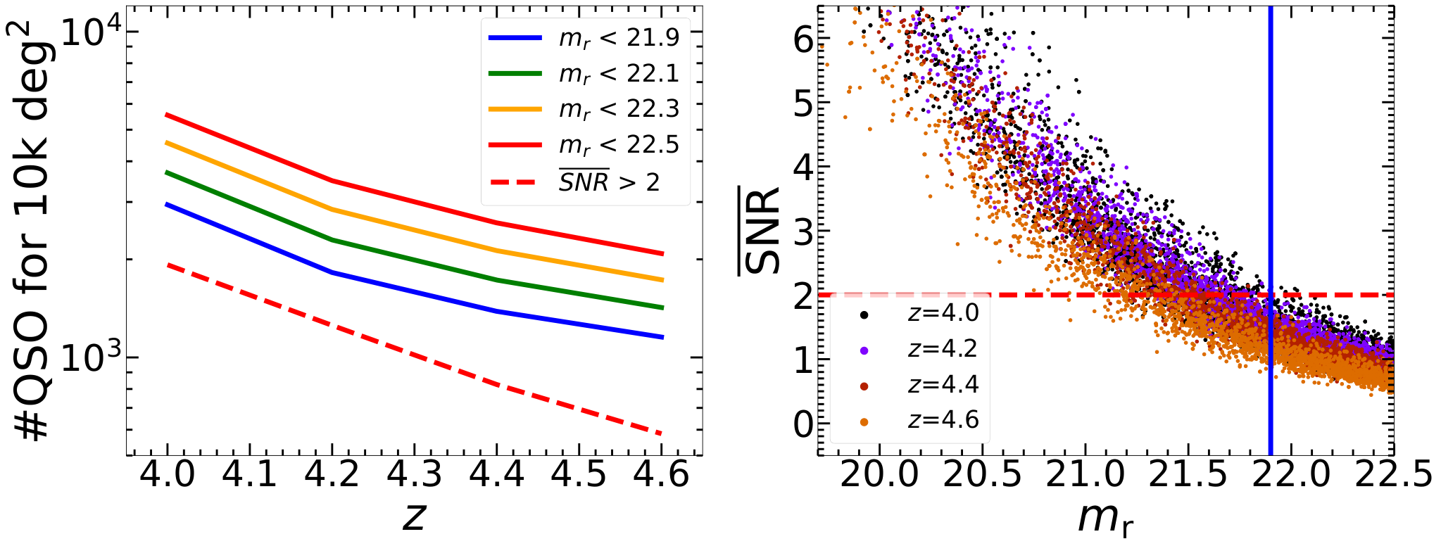
Using the procedure described in the previous section, for each of four redshift bins centered at and we generate mock QSO spectra that have systemic redshifts selected to have full spectral coverage within the bin. These bins target the redshift range where relic fluctuations from patchy reionization are expected to remain observable while retaining sufficient WEAVE-QSO sightlines for a useful forecast. The distributions of the quasar r-band magnitude, , and systemic redshift, , are sampled using a Monte Carlo method based on the QSO number density derived from the 55 luminosity function. We then scale this luminosity-function-based number density distribution to a reference forecast sample covering , applying the relevant and selections to obtain the expected QSO counts used below. For each set of mock QSO spectra, we also determine the fraction of QSOs in each redshift bin satisfying specific magnitude and signal-to-noise criteria (described below). These fractions are then scaled to obtain the total expected number of suitable QSOs across the full survey, as illustrated in the left panel of Figure 2.
The QSO sample cuts for are determined as follows. The r-band magnitude influences the noise level in the Ly forest region, which directly affects the measurement of . We quantify the noise in our mocks using , defined as the signal-to-noise ratio per Å averaged over all pixels within a given redshift bin. Previous studies of at (10; 64, e.g.,) have often applied cuts of 2 or 3 to mitigate noise. However, at the comparatively high redshifts considered in this work where the number of sufficiently bright QSOs is smaller, such cuts would drastically reduce the number of usable QSOs and increase the statistical uncertainty on . Hence, to maintain sample size while controlling noise, we therefore instead implement a cut in r-band magnitude. Specifically, we adopt for all redshift bins. As shown in the left panel of Figure 2, this magnitude cut retains over QSOs even in our highest redshift bin at . After applying the cut , we find the number of suitable QSOs in a survey is , , , and for redshift bins and respectively. We use these numbers throughout the rest of the paper, but in Section 4.2 we will briefly discuss how a smaller numbers of suitable QSOs (e.g., through incompleteness or reduced survey area) may impact on our forecast).
3 Power spectrum estimation
3.1 FFT estimator
We now discuss the calculation of the 1D power spectrum and its statistical and systematic uncertainties using our QSO survey mocks. The two approaches for computing the PLyα commonly used in the literature are the Fast Fourier Transform (56; 10; 64, FFT, e.g.) and the Quadratic Maximum Likelihood Estimator (36; 35, QMLE, e.g.). Although the latter benefits from being less sensitive to masking of the Ly forest spectrum, the former method is more straightforward. In addition, 64 and 35 measured the PLyα on the same DESI data sets using FFT and QMLE respectively, and found that the results are consistent within 1 per cent up to the half Nyquist frequency. We therefore use the FFT approach to measure .
When performing power spectra analysis, the commonly used estimator is the flux contrast , where
| (1) |
Here is the Ly transmission and is the mean transmission over some wavelength interval (which also depends on redshift). In this work we assume a mean transmission based on the Ly forest effective optical depth measurement presented by 2, where . The power spectrum is then given by
| (2) |
where represents the Fourier transform. In practice, is obtained by averaging the individual power spectra obtained from each of the QSO spectra within the redshift bin under consideration.
However, is not directly observable. Instead, the observed flux contrast, , is given by
| (3) |
where is the intrinsic QSO emission obtained from the continuum fitting procedure. For now we shall assume the QSO continuum is perfectly known, but we will return to modelling continuum fitting uncertainties later.
The underlying Ly flux contrast, , differs from the observed flux contrast, , due to instrumental resolution effects as well contamination by metal lines present in the Ly forest. The combination of these effects along with noise yields the observed flux. The relation between and can be expressed as,
| (4) |
where is the spectrograph line spread function as a function of wavelength , spectral resolution , and the pixel size . The terms and represent the contribution to the observed flux contrast by intervening metal lines and noise, respectively. The contribution from high column density systems is treated separately in Section 3.5.
After Fourier transforming Equation (4) using Equation (2), we obtain the relation between the observed power spectrum, , and the Ly forest power spectrum, :
| (5) |
One again, and represent the contribution to the observed power spectrum by metals and noise. We now turn to consider each of these components and their contribution to the measurement uncertainties in turn.
3.2 Spectrograph resolution correction
The WEAVE spectrograph low-resolution mode covers – at a representative resolving power of , while the high-resolution mode provides restricted wavelength coverage at (59; 32). The majority of QSO spectra in WEAVE-QSO will be obtained using the low-resolution mode. We assume in this work.
The WEAVEify package characterizes the effect of the spectrograph resolution using the line spread function matrix . As a forecast-level approximation, a Gaussian kernel is assumed with a standard deviation that varies as a function of wavelength, as detailed in Section 2.2. The square of the Fourier transform of this resolution matrix corresponds to the resolution correction factor that is applied to the power spectrum in Equation (5). The corresponding resolution windows for the four redshift bins we consider are shown in Figure 3; these remain very similar in all four bins. We use these correction factors to determine the -range impacted by instrument resolution and to estimate the contribution of the instrumental resolution correction to the final systematic uncertainty estimate. The maximum wavenumber, , for the measurements that we consider in this work is selected following the same criterion as the DESI collaboration (64), where is defined as the point beyond which the resolution correction falls below . This yields .
To estimate the uncertainty associated with applying this resolution correction, we draw bootstrap realizations of sight-lines from our mock spectra. For each realization, we compare the resolution corrected estimate with the underlying model and measure the scatter in their ratio across the bootstrap samples. The resulting term quantifies the residual uncertainty in the correction procedure. However, we note that this uncertainty quantifies the robustness of the correction for a fixed, known resolution window function. In a real WEAVE-QSO analysis, the resolving power will vary with wavelength and observing conditions, and uncertainty in will propagate into uncertainty in . This effect can become important near the high- limit of the measurement and should ultimately be treated using a wavelength-dependent resolution matrix or window-function uncertainty model. We discuss this further in Section 3.7.
3.3 Noise subtraction
The noise level is quantified by , the standard deviation of the flux. In observational studies, this quantity is typically estimated from the data reduction pipeline or using methods such as the exposure difference technique (10; 64, e.g.,). For our mock data, however, is directly provided as an output of the WEAVEify software. The standard deviation of the noise term in Equation (4) is thus defined as
| (6) |
In each redshift bin, for each pixel at wavelength we generate realizations of by drawing from a normal distribution with standard deviation . The noise power spectrum in Equation (5) is then estimated as , where the average is computed over all QSO spectra and realizations within the redshift bin. Note that the use of a normal distribution for generating reflects the assumption of Gaussian noise in WEAVEify. However, the noise model can be adapted as needed to match specific instrumental characteristics or data reduction pipelines.
Figure 4 displays the observed power spectra and the estimated noise power spectra for the four redshift bins considered in this work. The noise component becomes dominant beyond , which is also the wavenumber limit adopted for the spectral resolution correction. In a similar manner to the resolution correction uncertainty, we again estimate the uncertainty associated with noise subtraction using bootstrap realizations of sight-lines. For each realization, we compare the noise-subtracted power spectrum estimate with the corresponding noiseless mock estimate, and take the standard deviation of this correction ratio across bootstrap samples.
3.4 Metal absorption lines
The metal flux contrast, , consists of two components: one originating from intervening metal lines with rest frame wavelengths , and the other from metal lines that are correlated with the Ly forest with rest frame wavelengths . The first category includes C IV (1548, 1551), Si IV (1394, 1403), and Mg II (2796, 2804) which we will refer to as uncorrelated metals. The second category is dominated by Si III (1207) in our modeling, which we refer to as correlated metals. We have also tested Si II in this modelling framework, but found its contribution to be sub-percent over the range considered here; see 40 for further details.
In practice, the uncorrelated metal power spectrum, , is typically estimated using sidebands – spectral regions redward of the Ly rest frame wavelength that are devoid of Ly absorption (56; 10; 64). For this forecast, we generate the baseline Ly mock spectra without uncorrelated metal absorption and then add synthetic uncorrelated metal features separately to estimate and its contribution to the uncertainty budget. We do this following the approach of 71. We first estimate the number of absorption lines for each metal line species per unit redshift path length by integrating the appropriate column density distribution function (CDDF) (18; 19; 42) over the column density range cm-2. Using a Monte Carlo method, we draw column densities and line widths (with -parameter distributions from 28 assuming ) until the required number of metal lines is reached. These synthetic absorption features are then randomly inserted into the Ly forest region of each mock QSO spectrum. The CDDFs for C IV, Si IV, and Mg II doublets are modelled as power laws using the measurements from 18, 19, and 42, respectively. We use this to estimate the scale-dependent uncertainty associated with uncorrelated metal subtraction. The relative magnitude of compared with is shown in Figure 5. Although the contribution of can become relevant at very small scales, (71), at the larger scales of interest in this work it represents only a very small contribution to the total uncertainty (see Figure 9 later).
For the correlated metals, we generate Si III absorption spectra following the method described in 40. We assume the Si III optical depths scale as , where the silicon abundance [Si/H] is derived from the measurements of 66; 1 and the ionization fractions are computed using the photoionization code Cloudy (20; 11). Figure 6 illustrates the impact of Si III (1207) on and the characteristic oscillations that result (43, see also). Note, however, that correlated metals like Si III are typically not removed from analyses but are instead incorporated as additional fitting parameters. This is because their power spectrum, denoted here as , cannot be directly isolated from observations as their absorption lines are blended with the Ly forest. In this work, correlated metals are therefore not directly included in the systematic uncertainty estimate; instead, we assess in Section 4.1 whether omitting an explicit Si III model affects our parameter inference. For this purpose we use the four parameter model for Si III absorption recently introduced by 40. As we will discuss later, however, we find that the inclusion of the Si III in our mocks makes very little difference to our final results.
3.5 High column density systems
For the purpose of estimating the systematic uncertainty associated with incomplete absorber removal, we model high column density systems (HCDs), defined here as absorbers with neutral hydrogen column densities satisfying . These systems are highly relevant to this study because enhancements to the power spectrum on large scales can readily arise from column densities due to their extended Lorentzian damping wings. However, the observed incidence of these absorption lines is not captured in our hydrodynamical simulations; self-shielded gas with normalised density and is ignored due to the “Quick-Ly” implementation (72) used in Sherwood-Relics (47, see e.g. figure 1 in). We therefore incorporate these HCDs into our mock QSO spectra using a similar method to that employed for the uncorrelated metal lines. The column density distribution function from 61 is used to estimate the expected number of HCDs per unit redshift path length, which we then Monte Carlo sample over the range defined by 61 assuming a fixed Doppler parameter . The resulting synthetic HCD absorbers are inserted as Voigt profiles at locations where the Ly optical depth in our mock spectra is largest.
In practice, HCDs cannot be perfectly identified and removed from observational data. To assess the potential bias in resulting from incomplete removal, we use the completeness function from 74 for systems with . For each bin, we randomly remove HCDs according to this completeness function – considering our mean signal-to-noise ratio – and retain the remaining systems in the Ly forest region. The impact of HCDs on , both with and without incomplete removal, is illustrated in Figure 7. The systematic error introduced by the incomplete removal (solid curves) is added into the total uncertainty estimate in quadrature. For the incomplete-removal model shown in Figure 7, the residual HCD contribution to is at most per cent at , with the maximum occurring at the largest scales.
3.6 Continuum shape
In our mock QSO spectra a continuum template is assigned to each line of sight by WEAVEify and is subsequently divided out during the computation of (as described in Section 3.1). However, in practice the QSO continuum is not known and may be misplaced. As a conservative forecast-level test of this systematic effect, instead of dividing by the true continuum (which varies with wavelength) we divide the WEAVEified mocks by a flat, wavelength independent continuum and evaluate the resulting impact on . The flat continuum is defined as the mean value of the true continuum over the redshift bin covered by each mock QSO spectrum. This approach isolates shape related biases from normalization effects, which are instead marginalized over by varying the effective optical depth, , in our parameter inference procedure. The impact of an incorrect continuum shape on is shown in Figure 8. The associated systematic error is again added in quadrature to the total uncertainty estimate.
3.7 Final uncertainty estimate
We now combine our systematic uncertainty estimates with the expected statistical uncertainty from the WEAVE-QSO survey. Statistical uncertainties originate from finite sample sizes and are estimated relative to the mean . We use the predicted number of QSOs (denoted ) expected in a survey after applying an r-band cut of , as described in Section 2.4. For each of the four redshift bins considered here, we then generate bootstrap realizations of the mean by randomly sampling sightlines with replacement. The statistical errors are derived as the square root of the diagonal elements of the resulting covariance matrix.
Next, for systematics associated with spectral resolution, noise subtraction, and uncorrelated metals, we use the mock spectra to construct bootstrap estimates of the residual uncertainty associated with each correction. The corresponding quantities shown in Figure 9 are the standard deviations of the corresponding correction ratios across bootstrap realizations of randomly sampled sightlines. For HCDs and continuum placement, we estimate the uncertainty from the fractional change in . The HCD contribution is modelled using the ratio between power spectra with incomplete HCD removal and the pure Ly spectrum (solid curves in Figure 7). The continuum placement contribution is evaluated analogously (solid curves in Figure 8). The total systematic uncertainty is computed as the quadratic sum of all individual contributions. We note that the forecast uncertainty estimate assumes perfect knowledge of the spectral-resolution window and of the noise model. In real WEAVE-QSO data, uncertainties in both quantities will need to be tested carefully. We have tested the effect of including a 10 per cent uncertainty in , finding that the resulting fractional systematic uncertainty is roughly 25–50 per cent near , much larger than the current bootstrap resolution term and also larger than the noise term near . However, this contribution remains below 1 per cent at (and is per cent at ) and therefore does not affect the large-scale modes that dominate the patchy reionization detection forecast presented in this paper.
Figure 9 shows the resulting estimate for the 1 relative uncertainties. The statistical and systematic contributions are indicated by dotted and dashed lines, respectively, while the solid lines represent their quadratic sum. As before, the grey shaded region shows the maximum wavenumber for the measurements that we consider in this work, . The total systematic uncertainty at large reflects the dominance of the noise subtraction term on small scales, whereas the increase in the statistical error with redshift is due to the smaller number of QSOs in the higher redshift bins. At large scales (), the total uncertainties remain below 10 per cent for all redshift bins. The average uncertainty at over all four redshift bins is 5.2 per cent. Over the range , the relative uncertainties on are dominated by the statistical contribution (i.e. where the dotted line is above the dashed line in Figure 9). Within this range, we forecast an average relative uncertainty of 3.1 per cent. These estimates are used to construct the covariance matrix for a WEAVE-QSO measurement, which we now use as an input within our Markov Chain Monte Carlo (MCMC) parameter inference framework.
4 The imprint of patchy reionization at z>4
4.1 Parameter inference framework
We now use our mock 1D Ly power spectrum covariance matrix to test whether a WEAVE-QSO measurement can recover the large-scale imprint of patchy reionization. Our MCMC parameter inference framework follows the approach used in earlier work, where the measured is compared against a grid of simulated power spectra while marginalizing over astrophysical parameters (71; 29; 49, e.g.). For each redshift bin, our Ly forest model is described by the effective optical depth , the temperature at mean density , the slope of the temperature-density relation , and the cumulative thermal energy per unit mass (53). These parameters control the mean transmission and thermal state of the IGM, and hence the amplitude and shape of the intrinsic . We do not vary any cosmological parameters in this analysis (see 49, for further discussion of this point).
In addition, we include an extra parameter that describes the effect of patchy reionization on the Ly forest at . For this purpose we adopt the patchy reionization correction used by 49, based on the tabulated data presented in table 2 of 48. These corrections were calculated using the Sherwood-Relics simulation suite (62), by taking the ratio of obtained from hybrid radiative transfer simulations of patchy reionization to models using a spatially uniform UV background with the same volume averaged reionisation history as the patchy model. On the scales relevant for this work the correction enhances the large-scale power at , primarily due to spatial variations in the IGM ionization and thermal state that persist following the completion of reionization (9; 17; 48).
Following 49, we parameterize this patchy reionization correction using the dimensionless parameter, , where
| (7) |
and is the redshift at which the correction is linearly interpolated from table 2 of 48. We allow to vary over the range by linearly extrapolating to a lower and upper redshift limit of (i.e., for no correction) and , respectively. Note that is used only as a numerical parameter controlling the amplitude of the patchy correction and should not be interpreted as a measurement of the redshift of reionization. In our MCMC analysis we allow one independent parameter in each redshift bin.
We compare two classes of fit to the same mock data set, which we construct by applying our covariance matrix estimate to from the Sherwood-Relics model used in this work. To facilitate a direct comparison to the earlier work of 49, throughout we adopt the wavenumber binning introduced by 36 and add a Gaussian noise realization to drawn from the forecast covariance matrix. The first fit includes and therefore allows the large-scale patchy reionization correction to vary in each redshift bin. We add this to our simulated mocks such that and in the redshift bins at and , respectively. The second fit removes this degree of freedom by disabling the patchy reionization correction. In both cases, we apply a broad top-hat prior on spanning – times the reference effective optical depth, following 3. The thermal parameters , , and are assigned Gaussian priors centered on the reference thermal history of the Sherwood-Relics simulation used here, with a 10 per cent width in each redshift bin. We additionally impose a hard – consistency prior, analogous to the simulation-grid prior used by 49, to exclude thermal histories outside the modeled region. As both fits are applied to the same mock data the difference in the goodness-of-fit provides a test of the significance that a WEAVE-QSO measurement would favour an enhancement of large scale power from reionization.
Finally, we also include the impact of correlated Si III absorption following 40. As shown in Figure 6, the correlated Si III contribution has an oscillatory dependence on wavenumber. For the relatively sparse large-scale -binning that we adopt here, however, this oscillatory structure is always weakly sampled. Consequently we find negligible bias in the recovered posteriors when the Si III absorption model is included in our inference framework. We therefore do not consider this issue further.
| Run | Expected | Posterior peak | Best-fit | |
|---|---|---|---|---|
| Fiducial | 4.0 | 0.216 | 0.291 | |
| 4.2 | 0.294 | 0.289 | ||
| 4.4 | 0.373 | 0.400 | ||
| 4.6 | 0.451 | 0.462 | ||
| Loose thermal | 4.0 | 0.216 | 0.182 | |
| 4.2 | 0.294 | 0.266 | ||
| 4.4 | 0.373 | 0.473 | ||
| 4.6 | 0.451 | 0.388 | ||
| No lowest- bin | 4.0 | 0.216 | 0.291 | |
| 4.2 | 0.294 | 0.214 | ||
| 4.4 | 0.373 | 0.131 | ||
| 4.6 | 0.451 | 0.522 |
4.2 Recovery of the large scale power enhancement
Figure 10 shows the mock data in the four redshift bins considered in this work, together with the best-fit model predictions obtained from the MCMC analysis. Note again the uncertainties are derived from the uncertainty estimate summarised in Section 3.7. This comparison is performed using the same mock data set and covariance matrix for all fits, such that any difference in the likelihood is driven only by the model assumptions. The red solid curves show the fiducial fit in which one independent parameter is varied in each redshift bin. The blue dashed curves show the best-fit excluding the parameter while all other IGM parameters are allowed to vary as before (the posterior distributions for all parameters are provided in Appendix A).
For the combined fit across all four redshift bins, the fiducial model provides an acceptable fit to the mock, with . By contrast, disabling the patchy correction degrades the fit to . The improvement is for four additional patchy reionization amplitude parameters. Interpreting this likelihood ratio statistic using Wilks’ theorem gives , corresponding to a two-sided Gaussian-equivalent significance of for the fiducial patchy reionization model. Thus, even after allowing the no- fit to adjust the thermal and ionization parameters the mock data strongly prefer the additional large-scale correction associated with patchy reionization. This demonstrates the patchy reionization imprint inserted into the mock is not fully absorbed by variations in , , , or , and remains significant even after a detailed accounting of WEAVE-QSO survey uncertainties.
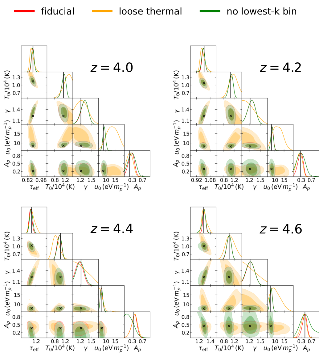
The posterior distributions for are displayed in Figure 11 and Table 1. In addition to the fiducial fit (red curves) here we consider two further cases. First, we repeat the analysis with broader thermal priors to test whether the inferred patchy reionization amplitudes are driven by restrictive assumptions about the IGM thermal state (orange curves). In this relaxed-prior run, we replace the fiducial Gaussian priors on , , and with broad top-hat priors over the simulation grid ranges, while keeping the same prior and the same – consistency cut. Specifically, we use and , with allowed to vary over the corresponding simulation-grid range in each redshift bin. Second, we remove the lowest- bin at from each redshift bin to test the sensitivity of the recovery to the largest scale mode included in the fit (green curves).
The fiducial analysis recovers the expected patchy amplitudes in all bins. In each case, the expected value lies within the 68 per cent credible interval of the posterior distribution. Relaxing the thermal parameter priors leads to minor shifts and slightly broader posteriors, but the expected values remain consistent with the inferred distributions. This indicates that the recovery is not simply imposed by restrictive priors on , , or the integrated thermal history. However, removing the lowest- bin from each redshift bin weakens the constraints. This is expected because the patchy reionization correction is largest on this scale. The posteriors broaden by factors of approximately 1.3–2.4 relative to the fiducial case. In the corresponding no-lowest- bin model comparison, the improvement from including is reduced to for four additional parameters, corresponding to a two-sided Gaussian-equivalent preference of only . In this case there is no longer a preference for large scale power enhancement from patchy reionization. Nevertheless, the expected values remain well recovered with the exception of the , where only an upper limit is obtained. This demonstrates that most of the constraining power on comes from retaining modes with . We also emphasise that the forecast uncertainties in the lowest- bins are dominated by the systematic uncertainty associated with damping wings from high column density absorbers and to a lesser extent the continuum placement. We have verified this remains the case even if lowering in each redshift bin by a factor of from our fiducial values. This implies that the WEAVE-QSO survey configuration of approximately with should comfortably exceed the minimum requirement on QSO sample size.
In summary, our results indicate a WEAVE-QSO measurement at with the forecast covariance adopted here can recover the redshift dependent patchy reionization amplitude at a two-sided Gaussian-equivalent significance of . This forecast significance is higher than the preference for additional large scale power reported by 49 from an analysis of the observed 1D power spectrum measurements presented by 36. While our analysis is based on mock WEAVE-QSO data with a forecast covariance, this comparison suggests that WEAVE-QSO should have sufficient statistical precision to turn the tentative evidence seen in current data into a significant detection of the large scale patchy reionization signature. However, the largest scale mode provides substantial constraining power: when the lowest- bin is removed, the model-comparison preference for including is weakened to and is no longer significant.
5 Summary and conclusions
In this work, we have developed a framework to forecast the sensitivity of a massive spectroscopic survey to the large-scale imprint of patchy hydrogen reionization in the one-dimensional Ly forest flux power spectrum, . We have opted to focus on a WEAVE-QSO survey configuration (59; 32), targeting four high-redshift bins of width centred at and , where relic temperature fluctuations from inhomogeneous reionization are expected to remain observable in (75; 48; 49). However, we anticipate that other current and forthcoming massive spectroscopic surveys that aim to constrain large-scale power in the Lyforest at wavenumbers at should also be capable of this novel measurement.
Our mock spectra are based on the Sherwood-Relics simulation suite (62) and are processed with the WEAVEify pipeline to include the main observational ingredients relevant for WEAVE-QSO spectra. We construct a realistic high-redshift QSO population using luminosity-function-based Monte Carlo sampling (55) and adopt an -band magnitude cut of . For a survey area, this selection yields expected QSO numbers of , , , and in the four redshift bins considered here.
We use our pipeline to quantify the overall uncertainty for a WEAVE-QSO measurement. The covariance matrix estimate includes statistical errors and systematic contributions from spectral resolution, noise subtraction, continuum misplacement, uncorrelated metal contamination, and the incomplete identification of high column density absorbers with . Within our adopted maximum wavenumber cut, , the estimated relative uncertainties remain below 10 per cent on the largest scales in all redshift bins. Averaged over all bins and scales below this cut, the total uncertainty is 5.2 per cent. Over the range , the uncertainties are dominated by the statistical contribution and the average uncertainty is 3.1 per cent.
Using this forecast covariance, we construct a mock data vector containing the fiducial patchy reionization signal and test whether it can be distinguished from an IGM that has been heated and ionised by a spatially uniform UV background. This inference test follows the patchy reionization parameterization and wavenumber binning used in earlier work (49). Allowing one independent patchy reionization amplitude parameter, , in each redshift bin improves the fit from to , corresponding to for four additional patchy amplitude parameters and a preference for additional power at large scales from patchy reionization. This result remains robust to changes in the prior adopted for IGM thermal parameters and is driven almost entirely by the lowest- bin from each redshift bin.
Our results indicate that a WEAVE-QSO measurement of the high-redshift Ly forest power spectrum should be capable of detecting and characterizing the large-scale relic imprint of patchy reionization, provided that the observational covariance is controlled at the level forecast here. More broadly, the framework developed in this work provides a route for assessing the sensitivity of current and future massive spectroscopic surveys to the timing of reionization through large-scale measurements.
Acknowledgements
KM gratefully acknowledges the financial support provided by the China Scholarship Council programme (Project ID: CSC NO. 202309110040). JSB is supported by STFC consolidated grant ST/X000982/1. The modelling in this work was performed using the Joliot Curie supercomputer at the Trés Grand Centre de Calcul (TGCC) and the DiRAC Data Intensive service (CSD3) at the University of Cambridge, managed by the University of Cambridge University Information Services on behalf of the STFC DiRAC HPC facility (www.dirac.ac.uk). We acknowledge the Partnership for Advanced Computing in Europe (PRACE) for awarding us time on Joliot Curie in the 16th call. The DiRAC component of CSD3 at Cambridge was funded by BEIS, UKRI and STFC capital funding and STFC operations grants. DiRAC is part of the National e-Infrastructure. We thank Volker Springel for making P-Gadget-3 available and Philip Parry for technical support.
Data Availability
All data and analysis code used in this work are available from the first author on reasonable request. Further guidance on accessing the publicly available Sherwood-Relics simulation data may also be found at https://www.nottingham.ac.uk/astronomy/sherwood-relics/.
References
- Metallicity of the Intergalactic Medium Using Pixel Statistics. III. Silicon. ApJ 602 (1), pp. 38–50. External Links: Document, astro-ph/0310664 Cited by: §3.4.
- A refined measurement of the mean transmitted flux in the Ly forest over 2 < z < 5 using composite quasar spectra. MNRAS 430 (3), pp. 2067–2081. External Links: Document, 1208.2584 Cited by: §2.3, §3.1.
- Revealing Reionization with the Thermal History of the Intergalactic Medium: New Constraints from the Ly Flux Power Spectrum. ApJ 872 (1), pp. 101. External Links: Document, 1809.06980 Cited by: §4.1.
- Resolving the high redshift Ly forest in smoothed particle hydrodynamics simulations. MNRAS 398 (1), pp. L26–L30. External Links: Document, 0906.2861 Cited by: §2.1.
- The Lyman forest opacity and the metagalactic hydrogen ionization rate at z~2-4. MNRAS 357 (4), pp. 1178–1188. External Links: Document, astro-ph/0411072 Cited by: §1.
- The Sherwood simulation suite: overview and data comparisons with the Lyman forest at redshifts 2 z 5. MNRAS 464 (1), pp. 897–914. External Links: Document, 1605.03462 Cited by: §1.
- The hydrodynamic response of small-scale structure to reionization drives large IGM temperature fluctuations that persist to z = 4. MNRAS 533 (1), pp. L100–L106. External Links: Document, 2405.02397 Cited by: §1.
- Observations of the spectra of Q0122-380 and Q1101-264.. MNRAS 198, pp. 91–110. External Links: Document Cited by: §2.3.
- Probing the Epoch of Reionization with the Ly Forest at z ~4-5. ApJ 706 (1), pp. L164–L167. External Links: Document, 0907.0735 Cited by: §1, §4.1.
- The one-dimensional power spectrum from the SDSS DR14 Ly forests. J. Cosmology Astropart. Phys. 2019 (7), pp. 017. External Links: Document, 1812.03554 Cited by: §1, §2.4, §3.1, §3.3, §3.4.
- The 2023 Release of Cloudy. Rev. Mex. Astron. Astrofis. 59, pp. 327–343. External Links: Document, 2308.06396 Cited by: §3.4.
- Cosmological analysis of the DESI DR1 Ly 1D power spectrum. J. Cosmology Astropart. Phys. 2026 (6), pp. 040. External Links: Document, 2601.21432 Cited by: §1.
- Toward a Precise Measurement of Matter Clustering: Ly Forest Data at Redshifts 2-4. ApJ 581 (1), pp. 20–52. External Links: Document, astro-ph/0012324 Cited by: §1.
- Predicting Quasar Continua Near Lyman- with Principal Component Analysis. arXiv e-prints, pp. arXiv:1801.07679. External Links: Document, 1801.07679 Cited by: §2.2.
- 4MOST: Project overview and information for the First Call for Proposals. The Messenger 175, pp. 3–11. External Links: Document, 1903.02464 Cited by: §1.
- The DESI Experiment Part I: Science,Targeting, and Survey Design. arXiv e-prints, pp. arXiv:1611.00036. External Links: Document, 1611.00036 Cited by: §1.
- Large Opacity Variations in the High-redshift Ly Forest: The Signature of Relic Temperature Fluctuations from Patchy Reionization. ApJ 813 (2), pp. L38. External Links: Document, 1509.02523 Cited by: §1, §4.1.
- Metals in the IGM approaching the re-ionization epoch: results from X-shooter at the VLT. MNRAS 435 (2), pp. 1198–1232. External Links: Document, 1306.4604 Cited by: §3.4.
- The evolution of the Si IV content in the Universe from the epoch of reionization to cosmic noon. MNRAS 512 (2), pp. 2389–2401. External Links: Document, 2202.12206 Cited by: §3.4.
- CLOUDY 90: Numerical Simulation of Plasmas and Their Spectra. PASP 110 (749), pp. 761–778. External Links: Document Cited by: §3.4.
- A consistent and robust measurement of the thermal state of the IGM at 2 z 4 from a large sample of Ly forest spectra: evidence for late and rapid He II reionization. MNRAS 506 (3), pp. 4389–4412. External Links: Document, 2009.00016 Cited by: §1.
- Constraining mixed dark matter models with high-redshift Lyman-alpha forest data. Phys. Rev. D 112 (4), pp. 043502. External Links: Document, 2504.06367 Cited by: §1.
- Post-inflationary axion constraints from the Lyman- forest. arXiv e-prints, pp. arXiv:2603.04401. External Links: Document, 2603.04401 Cited by: §1.
- The Prime Focus Spectrograph Galaxy Evolution Survey. arXiv e-prints, pp. arXiv:2206.14908. External Links: Document, 2206.14908 Cited by: §1.
- Small-scale structure and the Lyman- forest baryon acoustic oscillation feature. MNRAS 474 (2), pp. 2173–2193. External Links: Document, 1707.03358 Cited by: §1.
- One likelihood to bind them all: Lyman- constraints on non-standard dark matter. J. Cosmology Astropart. Phys. 2022 (10), pp. 032. External Links: Document, 2206.08188 Cited by: §1.
- The thermal memory of reionization history. The Astrophysical Journal 596 (1), pp. 9. External Links: Document, Link Cited by: §1.
- The b Distribution and the Velocity Structure of Absorption Peaks in the Ly Forest. ApJ 517 (2), pp. 541–548. External Links: Document, astro-ph/9709100 Cited by: §3.4.
- The Lyman forest power spectrum from the XQ-100 Legacy Survey. MNRAS 466 (4), pp. 4332–4345. External Links: Document, 1702.01761 Cited by: §1, §4.1.
- New constraints on the free-streaming of warm dark matter from intermediate and small scale Lyman- forest data. Phys. Rev. D 96 (2), pp. 023522. External Links: Document, 1702.01764 Cited by: §1.
- Unveiling dark matter free streaming at the smallest scales with the high redshift Lyman-alpha forest. Phys. Rev. D 109 (4), pp. 043511. External Links: Document, 2309.04533 Cited by: §1.
- The wide-field, multiplexed, spectroscopic facility WEAVE: Survey design, overview, and simulated implementation. MNRAS 530 (3), pp. 2688–2730. External Links: Document, 2212.03981 Cited by: §1, §1, §2.2, §3.2, §5.
- DESI DR1 Ly 1D power spectrum: The optimal estimator measurement. arXiv e-prints, pp. arXiv:2505.07974. External Links: Document, 2505.07974 Cited by: §1.
- Optimal 1D Ly forest power spectrum estimation - I. DESI-lite spectra. MNRAS 497 (4), pp. 4742–4752. External Links: Document, 2008.06421 Cited by: §1.
- Optimal 1D Ly forest power spectrum estimation - III. DESI early data. MNRAS 528 (3), pp. 3941–3963. External Links: Document, 2306.06316 Cited by: §1, §1, §3.1.
- Optimal 1D Ly forest power spectrum estimation - II. KODIAQ, SQUAD, and XQ-100. MNRAS 509 (2), pp. 2842–2855. External Links: Document, 2108.10870 Cited by: §1, §1, §3.1, §4.1, §4.2.
- Spatial fluctuations of the intergalactic temperature-density relation after hydrogen reionization. MNRAS 477 (4), pp. 5501–5516. External Links: Document, 1709.05351 Cited by: §1, §1.
- An improved measurement of the flux distribution of the Ly forest in QSO absorption spectra: the effect of continuum fitting, metal contamination and noise properties. MNRAS 382 (4), pp. 1657–1674. External Links: Document, 0711.1862 Cited by: §2.3.
- XQ-100: A legacy survey of one hundred 3.5 z 4.5 quasars observed with VLT/X-shooter. A&A 594, pp. A91. External Links: Document, 1607.08776 Cited by: §1.
- An improved model for the effect of correlated Si III absorption on the one-dimensional Lyman- forest power spectrum. MNRAS 546 (1), pp. staf2262. External Links: Document, 2509.08613 Cited by: §2.1, §3.4, §3.4, §4.1.
- The Wide-field Spectroscopic Telescope (WST) Science White Paper. arXiv e-prints, pp. arXiv:2403.05398. External Links: Document, 2403.05398 Cited by: §1.
- The Vulture Survey I: Analyzing the Evolution of Absorbers. arXiv e-prints, pp. arXiv:1701.05624. External Links: Document, 1701.05624 Cited by: §3.4.
- The Ly Forest Power Spectrum from the Sloan Digital Sky Survey. ApJS 163 (1), pp. 80–109. External Links: Document, astro-ph/0405013 Cited by: §3.4.
- The Linear Theory Power Spectrum from the Ly Forest in the Sloan Digital Sky Survey. ApJ 635 (2), pp. 761–783. External Links: Document, astro-ph/0407377 Cited by: §1.
- The Evolution of the Intergalactic Medium. ARA&A 54, pp. 313–362. External Links: Document, 1512.00086 Cited by: §1, §1.
- The physics of the intergalactic medium. Reviews of Modern Physics 81 (4), pp. 1405–1469. External Links: Document, 0711.3358 Cited by: §1, §1.
- Searching for the shadows of giants: characterizing protoclusters with line of sight Lyman- absorption. MNRAS 489 (4), pp. 5381–5397. External Links: Document, 1909.02513 Cited by: §3.5.
- The effect of inhomogeneous reionization on the Lyman forest power spectrum at redshift z > 4: implications for thermal parameter recovery. MNRAS 509 (4), pp. 6119–6137. External Links: Document, 2109.06897 Cited by: §1, §1, §4.1, §4.1, §5.
- Possible evidence for a large-scale enhancement in the Lyman- forest power spectrum at redshift z 4. MNRAS 521 (1), pp. 1489–1501. External Links: Document, 2303.05167 Cited by: §1, §4.1, §4.1, §4.1, §4.1, §4.2, §5, §5.
- Extracting the astrophysics of reionization from the Ly forest power spectrum: a first forecast. MNRAS 508 (1), pp. 1262–1279. External Links: Document, 2106.14492 Cited by: §1.
- Absorption Spectrum of the Z = 3.78 QSO 2000-330. II. The Redshift and Equivalent Width Distributions of Primordial Hydrogen Clouds. ApJ 309, pp. 19. External Links: Document Cited by: §2.3.
- The UVES Spectral Quasar Absorption Database (SQUAD) data release 1: the first 10 million seconds. MNRAS 482 (3), pp. 3458–3479. External Links: Document, 1810.06136 Cited by: §1.
- Inferring the IGM thermal history during reionization with the Lyman forest power spectrum at redshift z ≃ 5. MNRAS 463 (3), pp. 2335–2347. External Links: Document, 1605.04155 Cited by: §4.1.
- The First Data Release of the KODIAQ Survey. AJ 150 (4), pp. 111. External Links: Document, 1505.03529 Cited by: §1.
- The extended Baryon Oscillation Spectroscopic Survey: Variability selection and quasar luminosity function. A&A 587, pp. A41. External Links: Document, 1509.05607 Cited by: Figure 2, §2.4, §5.
- The one-dimensional Ly forest power spectrum from BOSS. A&A 559, pp. A85. External Links: Document, 1306.5896 Cited by: §1, §1, §3.1, §3.4.
- A principal component analysis of quasar UV spectra at z ~3. A&A 530, pp. A50. External Links: Document, 1104.2024 Cited by: §2.2.
- Constraints on primordial magnetic fields from the lyman- forest. Phys. Rev. Lett. 135, pp. 071001. External Links: Document, Link Cited by: §1.
- WEAVE-QSO: A Massive Intergalactic Medium Survey for the William Herschel Telescope. In SF2A-2016: Proceedings of the Annual meeting of the French Society of Astronomy and Astrophysics, C. Reylé, J. Richard, L. Cambrésy, M. Deleuil, E. Pécontal, L. Tresse, and I. Vauglin (Eds.), pp. 259–266. External Links: Document, 1611.09388 Cited by: §1, §2.2, §3.2, §5.
- Automated quasar continuum estimation using neural networks: A comparative study of deep-learning architectures. A&A 698, pp. A292. External Links: Document, 2505.10976 Cited by: §2.2.
- Towards a unified description of the intergalactic medium at redshift z 2.5. MNRAS 438 (1), pp. 476–486. External Links: Document, 1310.0052 Cited by: §3.5.
- The Sherwood-Relics simulations: overview and impact of patchy reionization and pressure smoothing on the intergalactic medium. MNRAS 519 (4), pp. 6162–6183. External Links: Document, 2207.13098 Cited by: §1, Figure 1, §2.1, §4.1, §5.
- The Opacity of the Ly Forest and Implications for and the Ionizing Background. ApJ 489 (1), pp. 7–20. External Links: Document, astro-ph/9612245 Cited by: §1.
- The Dark Energy Spectroscopic Instrument: one-dimensional power spectrum from first Ly forest samples with Fast Fourier Transform. MNRAS 526 (4), pp. 5118–5140. External Links: Document, 2306.06311 Cited by: §1, §1, §2.4, Figure 3, §3.1, §3.2, §3.3, §3.4.
- 5 tension between Planck cosmic microwave background and eBOSS Lyman-alpha forest and constraints on physics beyond CDM. Physical Review Research 7 (1), pp. L012018. External Links: Document, 2311.16377 Cited by: §1.
- Metallicity of the Intergalactic Medium Using Pixel Statistics. II. The Distribution of Metals as Traced by C IV. ApJ 596 (2), pp. 768–796. External Links: Document, astro-ph/0306469 Cited by: §3.4.
- The thermal history of the intergalactic medium. MNRAS 318 (3), pp. 817–826. External Links: Document, astro-ph/9912432 Cited by: §1.
- The cosmological simulation code GADGET-2. MNRAS 364 (4), pp. 1105–1134. External Links: Document, astro-ph/0505010 Cited by: §2.1.
- The BarYon Cycle project (ByCycle): identifying and localizing Mg II metal absorbers with machine learning. MNRAS 526 (3), pp. 3744–3756. External Links: Document, 2305.17970 Cited by: §1.
- Constraints on reionization from the thermal history of the intergalactic medium* **. The Astrophysical Journal 567 (2), pp. L103. External Links: Document, Link Cited by: §1.
- Warm dark matter as a solution to the small scale crisis: New constraints from high redshift Lyman- forest data. Phys. Rev. D 88 (4), pp. 043502. External Links: Document, 1306.2314 Cited by: §3.4, §4.1.
- Inferring the dark matter power spectrum from the Lyman forest in high-resolution QSO absorption spectra. MNRAS 354 (3), pp. 684–694. External Links: Document, astro-ph/0404600 Cited by: §1, §3.5.
- New constraints on warm dark matter from the Lyman- forest power spectrum. Phys. Rev. D 108 (2), pp. 023502. External Links: Document, 2209.14220 Cited by: §1.
- Deep Learning of Dark Energy Spectroscopic Instrument Mock Spectra to Find Damped Ly Systems. ApJS 259 (1), pp. 28. External Links: Document, 2201.00827 Cited by: Figure 7, §3.5.
- Imprints of temperature fluctuations on the z 5 Lyman- forest: a view from radiation-hydrodynamic simulations of reionization. MNRAS 490 (3), pp. 3177–3195. External Links: Document, 1907.04860 Cited by: §1, §1, §5.
- MUltiplexed survey telescope: perspectives for large-scale structure cosmology in the era of stage-v spectroscopic survey. External Links: 2411.07970, Link Cited by: §1.
- Tantalizing evidence of reionization relics in the eBOSS DR16 Ly forest correlations: a preference for early reionization. MNRAS 545 (4), pp. staf2014. External Links: Document, 2503.09971 Cited by: §1.
Appendix A Posterior distributions
Figures 12 and 13 show the marginalized posterior distributions for all five parameters (, , , , ) varied in each redshift bin. Figure 12 corresponds to the best fit displayed in Figure 10, while Figure 13 corresponds to the 1D posteriors displayed in Figure 11.