R-estimation in a Linear Model with Autoregressive Errors

Classical regression methods, such as Ordinary Least Squares (OLS), often fail in the presence of outliers or autocorrelated error structures. These conditions are common in practice, yet often remain undetected in observational data. As a result, standard estimation procedures can lead to misleading conclusions — for instance, they may mask an upward trend in hydrological or economic applications.

To address this, robust alternatives are needed that remain valid under such departures from ideal assumptions. In particular, the presence of autocorrelation in model errors can distort inference on regression parameters unless explicitly accounted for. In this paper, we propose a novel rank-based estimator that is invariant to both nuisance autoregression parameters and the intercept, while preserving desirable asymptotic properties. This estimator builds upon and extends the ideas of Jaeckel [9] and Koul and Saleh [28], and is particularly suited to models where errors follow an unknown autoregressive structure.

We consider a linear regression model of order $s$, where the model errors follow a stationary autoregressive process of order $p$:

Here, $y_{t}$ is the response variable, $\mathbf{x}_{t}=(x_{t1},\ldots,x_{ts})^{\top}$ are the regressors, and $\beta_{j}$, $j=1,\ldots,s$ are the unknown regression parameters, with $\beta_{0}$ as the intercept. Moreover, $\phi_{0},\phi_{1},\ldots,\phi_{p}$ are the unknown autoregressive parameters, where $\phi_{0}$ is included for mathematical convenience and may be zero. The parameters $\beta_{0}$ and $\beta$ are of primary interest, while $\phi_{0},\ldots,\phi_{p}$ are considered nuisance parameters. The innovations $u_{t}$ are assumed to be independent and identically distributed (i.i.d.) with a continuous distribution function $F(u)$, increasing on the set $\{u:0<F(u)<1\}$, and with density $f(u)$, which is generally unknown but satisfies:

We assume that the error process given in equation (1.1) is strictly stationary, so that the errors $\varepsilon_{t}$ share a common marginal distribution and, in particular, the same quantiles. The observable variables are $y_{t}$, for $t=0,\pm 1,\pm 2,\ldots$. For identifiability, we assume that the initial values $(y_{-p+1},\ldots,y_{0})$ are known.

Hallin and Jurečková [8] considered the autoregressive model without a nuisance linear regression and constructed an asymptotically optimal rank test for hypotheses concerning the autoregression parameters $\phi_{0},\ldots,\phi_{p}$. If the autoregression is treated as a nuisance and our inference focuses on the linear regression, then its presence can distort the conclusions drawn from the data. For example, it may lead to a false detection of a linear trend in water flow, or may mask a true trend.

Keeping this in mind, Jurečková et al. [15] proposed a nonparametric test of the hypothesis $\mathbf{H}_{0}:\mbox{\boldmath$\beta$}=\mathbf{0}$ that is invariant to the nuisance autoregression. Their main tool was the concept of autoregression rank scores, introduced by Koul and Saleh [28] as the dual counterpart to the autoregression quantile. These rank scores themselves are invariant to the nuisance autoregression, which ensures the invariance of the test statistic’s distribution under the null hypothesis.

However, the invariance of the test criterion under the null hypothesis is not sufficient for constructing a point estimator of $\beta$ when other parameters remain unspecified. Therefore, it is necessary to study the behavior of the test criterion in a neighborhood of the null hypothesis. This is addressed in the present paper, where we show that the linear autoregression rank statistic is asymptotically linear in the regression parameter. This property enables us to construct an invariant estimator of $\beta$, which corresponds to a nonparametric rank estimator (R-estimator). To adapt the rank-based approach to the autoregressive setting, the ranks of the residuals $y_{t}-\mathbf{x}_{t}^{\top}\mathbf{b}$ are replaced by the autoregression rank scores of these residuals. The resulting estimators of $\beta$ will be referred to as RR-estimators.

The problem of estimating the autoregression parameters themselves is not addressed in this paper. It has been studied, for example, in [27], [28], [26], [17], among others — typically without considering an additional linear regression. A linear programming estimator of the autoregression parameters, convenient in cases with heavy-tailed errors, was proposed in [3]. With respect to hypothesis testing, [16] proposed a test for serial independence in a linear model against potential autoregressive error structures. However, the problem of point estimation of autoregression parameters in the presence of an additional nuisance regression remains open, despite its clear relevance in applications.

This paper is organized as follows. Section 2 briefly reviews the concepts of autoregression quantiles and autoregression rank scores, along with their key properties (for further details, see [28], [8], [4], [18]), and , [14]. In Section 3, we define the RR-estimator of the regression parameter $\beta$ and illustrate its properties. Analogously to the rank estimators in models with i.i.d. errors, the RR-estimator is defined as a minimizer of a specific form of Jaeckel’s rank dispersion measure [9].

Section 4 presents a simulation study that compares the proposed RR-estimator with OLS and median quantile regression under various error distributions, including normal, contaminated normal, and Cauchy. Section 5 provides a numerical illustration using real-world data on real estate prices, demonstrating the robustness and practical applicability of the RR-estimator in comparison to classical and quantile-based methods.

Assume first that the observations $y_{t}$ follow the autoregressive (AR) model

with i.i.d. errors $u_{t}$. Denote the vectors

and consider the ($n\times p$ and $n\times(p+1)$, respectively) random matrices

The $\alpha$-autoregression quantile is defined as the solution

where $\widehat{\rho}^{0}_{n}(\alpha)\in\mathbb{R}$ and $\widehat{\mbox{\boldmath$\rho$}}^{1}_{n}(\alpha)\in\mathbb{R}^{p}$, obtained by minimizing over $\mathbf{r}=(r_{0},\mathbf{r}_{1}^{\top})^{\top}\in\mathbb{R}^{p+1}$ the objective function

Let $\mbox{\boldmath$\Sigma$}_{n}$ and $\mbox{\boldmath$\Sigma$}_{n}^{*}$ denote the empirical covariance matrices

Under regularity conditions (F1–F2) and (X1–X3) stated below, there exist positive definite matrices $\Sigma$ and $\mbox{\boldmath$\Sigma$}^{*}$ of respective orders $p\times p$ and $(p+1)\times(p+1),$ such that

The definition in (2.2) formally coincides with the classical regression quantile of Koenker and Bassett. Analogously, the dual linear programming formulation can be written as:

The solution $\widehat{\mathbf{a}}_{n}(\alpha)$, referred to as the vector of autoregression rank scores (ARS), is autoregression invariant, hence independent of the nuisance autoregression parameters$\phi_{1},\ldots,\phi_{p}$. In the special case where $\phi_{1}=\ldots=\phi_{p}=0$, the components $\widehat{a}_{t}(\alpha)$ coincide with the classical Hájek rank scores [7]:

where $R_{n,t}$ denotes the rank of $y_{t}$ among $\{y_{1},\ldots,y_{n}\}$.

Since $\widehat{\mbox{\boldmath$\rho$}}_{n}(\alpha)$ and $\widehat{\mathbf{a}}_{n}(\alpha)$ are dual to each other, their relationship satisfies:

To study the behavior of these quantities, we assume that the unknown density $f$ of $u_{t}$ belongs to the family $\mathcal{F}$ of exponentially tailed distributions satisfying:

1. (F1)

   $f$ is positive, absolutely continuous, and has finite Fisher information:

   $$\mathcal{I}(f)=\int\left(\frac{f^{\prime}(x)}{f(x)}\right)^{2}f(x)\,dx<\infty.$$

   Additionally, there exists $K_{f}\geq 0$ such that $f^{\prime}$ and $f^{\prime\prime}$ are bounded for all $|x|>K_{f}$.

2. (F2)

   $f(x)\to 0$ monotonically as $x\to\pm\infty$ and the distribution function $F$ satisfies:

   $$\lim_{x\to-\infty}\frac{-\log F(x)}{c|x|^{r}}=\lim_{x\to\infty}\frac{-\log(1-F(x))}{c|x|^{r}}=1,$$

   for some $c>0$ and $r\geq 1$.

Further consequences of (F1) and (F2) are detailed in [8] and [4].

In what follows, we denote by $\mathbf{X}_{n}$ the $n\times s$ regression matrix formed by stacking the regressors from model (1.1), that is,

Moreover, the following standard conditions are imposed on this matrix $\mathbf{X}_{n}$:

1. (X1)

   The matrix $\mathbf{A}_{n}=n^{-1}\mathbf{X}_{n}^{\top}\mathbf{X}_{n}$, of order $s\times s$, is positive definite for $n\geq n_{0}$.

2. (X2)

   $n^{-1}\sum_{t=1}^{n}\|\mathbf{x}_{t}\|^{4}=O(1)$ as $n\to\infty$.

3. (X3)

   $\lim_{n\to\infty}\max_{1\leq t\leq n}\left\{n^{-1}\mathbf{x}_{t}^{\top}\mathbf{A}_{n}^{-1}\mathbf{x}_{t}\right\}=0$.

Let $\mathbf{D}_{n}$ and $\mathbf{Q}_{n}$ denote the following two matrices, of respective orders $(s+1)\times(s+1)$ and $s\times s$:

We assume that

where $\mathbf{D}$ and $\mathbf{Q}$ are positive definite matrices of the same respective orders.

Our goal is to estimate the parameter $\beta$ by a suitable rank estimate. To proceed, fix an $\alpha\in(0,1)$, possibly around 1/2, and consider a nondecreasing score generating function

If we are not aware of autocovariances between the model errors, we normally use the nonparametric R-estimator of $\beta$, introduced in [10] and [25]; for its further study we refer to [19], [17], [20], among others. Let $R_{nt}({\mathbf{y}}-{\mathbf{X}}{\mathbf{b}})$ denote the rank of residual $y_{t}-{\mathbf{x}}_{t}^{\top}{\mathbf{b}}$, among $\left(y_{1}-{\mathbf{x}}_{1}^{\top}{\mathbf{b}},\ldots,y_{n}-{\mathbf{x}}_{n}^{\top}{\mathbf{b}}\right)$, for ${\mathbf{b}}\in{I\kern-3.69995ptR}^{s}$. The R-estimator, denoted $\check{\mbox{\boldmath$\beta$}}_{nR}(\alpha)$, is defined as a minimizer of the following Jaeckel [9] criterion ${\cal D}_{n}$, over ${\mathbf{b}}\in{I\kern-3.69995ptR}^{s}$:

Such estimator $\check{\mbox{\boldmath$\beta$}}_{nR}(\alpha)$ in fact estimates only the slope components
$\mbox{\boldmath$\beta$}=(\beta_{1},\ldots,\beta_{s})^{\top}.$ It is invariant to $\beta_{0}$ and does not depend on the value of quantile $F^{-1}(\alpha).$ The additional intercept component of the estimator will be the $[n\alpha]$-quantile $\check{\beta}_{n0}$ of $y_{1}-\mathbf{x}_{1}^{\top}\check{\mbox{\boldmath$\beta$}}_{nR,\alpha},\ldots,y_{n}-\mathbf{x}_{n}^{\top}\check{\mbox{\boldmath$\beta$}}_{nR,\alpha}$.

However, such estimator is still affected by the possible nuisance autoregression of model errors. In order to reduce this effect, we get an inspiration from the test of the hypothesis $\mathbf{H}_{0}:\{\mbox{\boldmath$\beta$}=\mathbf{0}\}$, developed in [15]; its test criterion is based on the linear autoregression rank score statistic. We can consider the test of hypothesis $\mathbf{H}_{\mathbf{b}}:\{\mbox{\boldmath$\beta$}=\mathbf{b}\}$ analogously, for any fixed $\mathbf{b}\in I\kern-3.69995ptR^{s}$. Such test would be based on the ranks of residuals $\tilde{y}_{t,\mathbf{b}}=y_{t}-\mathbf{x}_{t}^{\top}\mathbf{b},$ which under validity of the hypothesis $\mathbf{H}_{\mathbf{b}}$ would satisfy $\tilde{y}_{t,\mathbf{b}}=\beta_{0}+\varepsilon_{t},\;t=0,\pm 1,\pm 2,\ldots.$ Because the $\varepsilon_{t},\;t=0,\pm 1\pm 2,\ldots$ follow the autoregression model of the assumed order $p$, the residuals $\tilde{y}_{t,\mathbf{b}}$ will follow, under validity of $\mathbf{H}_{\mathbf{b}}$, the model

To profit from the invariance of the autoregression rank scores, we use them instead of the ranks of residuals. Hence we calculate the $\alpha$-autoregression rank scores

for the residuals/pseudo-observations $\tilde{y}_{t,\mathbf{b}}=y_{t}-\mathbf{x}_{t}^{\top}\mathbf{b}$, ongoingly for $\mathbf{b}\in I\kern-3.69995ptR^{s},\quad t=1,\ldots,n.$ As an estimator of $\beta$ we propose $\widetilde{\mbox{\boldmath$\beta$}}_{n\alpha}$ of the following modification of the Jaeckel measure of the rank dispersions:

Every point $\mathbf{b}=\widetilde{\mbox{\boldmath$\beta$}}_{nR}(\alpha)$ satisfying (3.4) is considered as a possible estimator of $\mbox{\boldmath$\beta$}.$ The measure $\mathcal{D}_{n}(\mathbf{b})$, based on the autoregression rank scores, is invariant to the autoregression parameters. Following [9], we see that it is a continuous, convex and piecewise linear function of $\mathbf{b}\in I\kern-3.69995ptR^{s}$. As such, it is differentiable in $\mathbf{b}$ a.e.; we can write

at any point of differentiability of $\mathcal{D}_{n}$.

Next we proceed as follows: Consider the residuals $\tilde{\mathbf{y}}_{n,\mathbf{b}}=\mathbf{y}_{n}-\mathbf{X}_{n}\mathbf{b},\;\mathbf{b}\in I\kern-3.69995ptR^{s}$, and for them calculate the $\alpha$-regression quantile and $\alpha$-regression rank scores. These two entities are dual to each other, hence they are in the relation

We propose the estimator $\widetilde{\mbox{\boldmath$\beta$}}_{nRR}(\alpha)\in{I\kern-3.69995ptR}^{s}$ of $\beta$, as a minimizer of the modification of Jaeckel [9] measure of the rank dispersion, with the $\alpha$-autoregression rank scores inserted; the modified measure has the form

Note that $\bar{a}_{n\alpha}=\frac{1}{n}\sum_{t=1}^{n}\hat{a}_{t\alpha}(\mathbf{y}_{n}-\mathbf{x}_{n}^{\top}\mathbf{b})$ is constant in $\mathbf{b}$, as an average of the AR rank scores. It implies that the solution of (3.6) is invariant to the intercept and to the nuisance autoregression parameters $\phi_{1},\ldots,\phi_{p}$.

The subgradient of (3.6) is the linear autoregression rank score statistic

Hence, the estimate $\widetilde{\mbox{\boldmath$\beta$}}_{n,RR}$ of $\beta$ can be alternatively expressed as a solution of the minimization

Because the building stones of $\widetilde{\mbox{\boldmath$\beta$}}_{n,RR}$ are invariant to the autoregression parameters and to the intercept, the resulting estimator is equally invariant. We can verify its consistency and other asymptotic properties, following up the approach for R-estimation in [13] and [20], with application of the results in [28] and [8]. This is detailed below. The method is based on the asymptotic linearity of the autoregression rank score statistics.

To further evaluate the performance of the proposed RR-estimator, we conducted a simulation study in a linear regression model with autoregressive errors. We compared its performance to the classical Ordinary Least Squares (OLS) estimator and the median Quantile Regression (QR) estimator. The model considered was:

where the errors follow an AR(1) process:

with $\phi=0.7$ and innovations $u_{t}$ generated from three different distributions:

1. 1.

   Standard normal: $u_{t}\sim\mathcal{N}(0,1)$,

2. 2.

   Contaminated normal: $u_{t}\sim 0.9\,\mathcal{N}(0,1)+0.1\,\mathcal{N}(0,25)$,

3. 3.

   Cauchy: $u_{t}\sim\text{Cauchy}(0,1)$.

The true parameter values were set as $\beta_{0}=1$, $\beta_{1}=2$, $\beta_{2}=-1$, and $\beta_{3}=0.5$. The covariates $x_{tj}$ were generated independently from $\mathcal{N}(0,1)$ for $j=1,2,3$, and the sample size was fixed at $n=100$. Each setting was replicated $1000$ times.

For each scenario, we computed the average bias and Root Mean Squared Error (RMSE) of the estimated coefficients across the 1000 replications. Table 1 summarizes the results.

Figures 1 and 2 provide visual summaries of the RMSE and bias, respectively, across all three estimators and distributions.

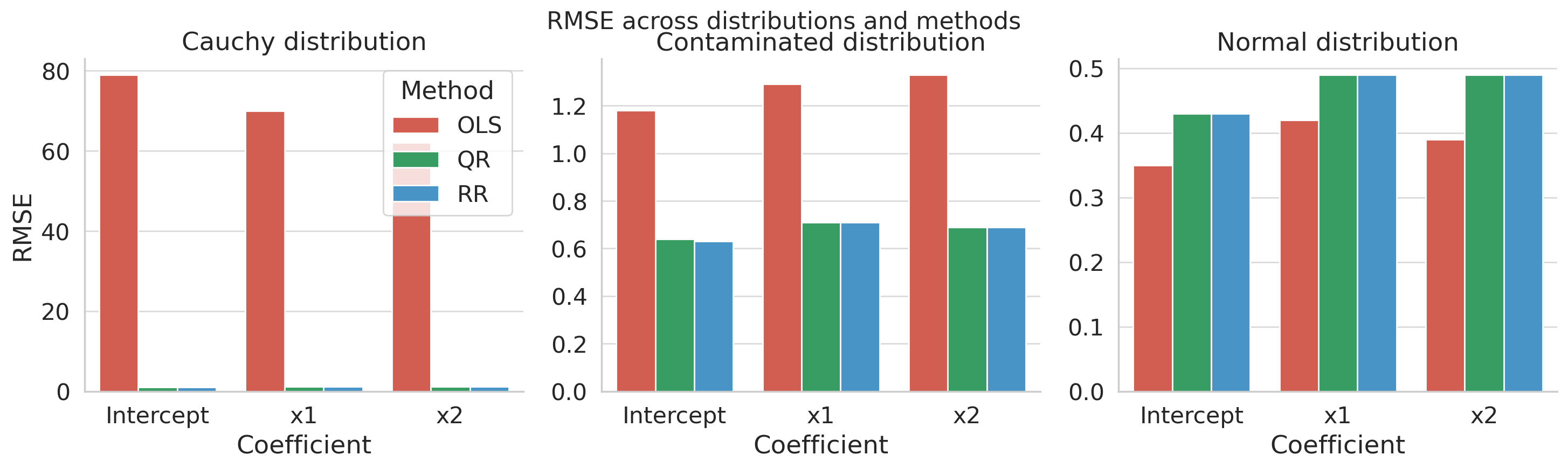
These results demonstrate that while OLS performs well under Gaussian errors, it is highly sensitive to contamination and heavy tails. Both QR and RR estimators offer substantially improved robustness in such cases. The RR-estimator often yields slightly lower RMSE than QR, confirming its competitiveness in scenarios with autoregressive and nonstandard error structures.

To complement the theoretical properties of the RR-estimator, we now demonstrate its behavior on a real-world data set. Specifically, we analyze the well-known real estate valuation data, originally collected by the Statistical Office of Taiwan and publicly available as “Real estate valuation data set.xlsx” [32]. The data consist of 414 observations and include explanatory variables such as the age of the house, the distance to the nearest MRT station, and the number of convenience stores within walking distance. The response variable is the price of a housing unit per square meter (expressed in NT$10000/m²).

We consider the following linear regression model:

where the error term $\varepsilon_{t}$ may exhibit an autoregressive structure or other forms of deviation from standard assumptions. The parameters were estimated using three different approaches:

1. 1.

   Ordinary Least Squares (OLS),

2. 2.

   Quantile Regression (QR) for $\tau=0.5$,

3. 3.

   Rank-based RR-estimator with $\alpha=0.5$.

The estimation was performed using the R packages quantreg [21] and readxl, with the RR-estimator computed by exploiting the dual solution of the quantile regression problem with $\tau=-1$.

Table 2 presents the parameter estimates obtained by the three methods. The estimates are relatively stable across all methods, indicating robustness of the linear relationship. However, some differences can be observed.

The intercept shows a noticeable downward shift when switching from OLS to QR and RR, which is expected given that QR and RR are less sensitive to potential skewness or outliers in the response variable. The slopes for all covariates remain close across the methods, with the RR estimates being generally closer to QR than to OLS, reflecting their shared robustness properties. In particular, the estimate for the number of convenience stores is slightly higher for QR and RR compared to OLS, suggesting that the influence of this variable may be more pronounced in the central part of the conditional distribution.

Figures 3 and 4 provide a graphical comparison between the observed and fitted house prices. The faceted version helps assess each method’s fit individually, while the overlaid version allows direct comparison. All three models show good alignment with the identity line, indicating reasonable predictive accuracy. However, the QR and RR methods tend to perform slightly better in the presence of extreme values, as expected due to their robustness.

The RR and QR estimates demonstrated improved performance over OLS in terms of both RMSE and MAE (Mean Absolute Error) on the test set, highlighting their advantage in cases with non-normal or heteroskedastic errors.

These findings support the usefulness of the RR-estimator in situations where the error structure might deviate from the classical assumptions, while maintaining reasonable efficiency and interpretability.

In this paper, we have introduced a novel rank-based estimator (RR-estimator) for the regression parameters in a linear model with autoregressive errors. Unlike classical methods such as Ordinary Least Squares (OLS), the RR-estimator remains robust under heavy-tailed error distributions, contamination, and nuisance autoregressive dependencies. In contrast to median Quantile Regression (QR), the RR-estimator is specifically adapted to the presence of serial correlation, providing invariance not only to distributional deviations but also to structural error dependence.

The RR-estimator inherits desirable theoretical properties, including asymptotic normality and efficiency under a broad class of error distributions. Practically, it offers greater stability in contaminated or heavy-tailed settings without requiring explicit modeling of the autoregression. Compared to QR, it provides an elegant alternative when serial dependence is suspected but the autoregressive structure is not explicitly specified or reliably estimated.

Our simulation studies and real-data applications demonstrate that the RR-estimator achieves comparable efficiency to QR under normal errors and superior robustness under contamination or heavy-tailed innovations. It consistently outperforms OLS, particularly in non-ideal conditions that frequently arise in applied fields such as hydrology and economics.

References

- [1] Alpuim, T. & El-Shaarawi, A., On the efficiency of regression analysis with AR(p) errors, J. Applied Statistics 35, 717–737 (2008)
- [2] Denby, L. and D. Martin, Robust estimation of the first order autoregressive parameter. J. Amer. Statist. Assoc. 74 : 140–146 (1979).
- [3] Feigin, P. D., Resnick, S. I., Limit distributions for linear programming time series estimators. Journal of Stochastic Processes & Applications 51, 135–65 (1994).
- [4] Güney, Y., Jurečková, J. and Arslan, O., Averaged Autoregression Quantiles in Autoregressive Model. In: Analytical Methods in Statistics (M. Maciak et al., Eds.), Springer Proceedings in Mathematics and Statistics Vol. 329, pp. 1–15 (2020), ISBN 978-3-030-48813-0.
- [5] Gutenbrunner, C. and Jurečková, J., Regression rank scores and regression quantiles, Ann. Statist. 20, 305–330 (1992).
- [6] Gutenbrunner, C., Jurečková, J., Koenker, R. and Portnoy, S., Tests of linear hypotheses based on regression rank scores, J. Nonpar. Statist. 2, 307-331 (1993).
- [7] Hájek, J., Extension of the Kolmogorov-Smirnov test to regression alternatives. Bernoulli-Bayes-Laplace (L. Le Cam and J. Neyman, eds), 45-60. Springer-Verlag, New York (1965).
- [8] Hallin, M. and Jurečková, J., Optimal tests for autoregressive models based on autoregression rank scores, Ann. Statist. 27, 1385–1414 (1999).
- [9] Jaeckel, L. A. , Estimating regression coefficients by minimizing the dispersion of the residuals. Ann. Math. Statist. 43, 1449–1459 (1972).
- [10] Jurečková, J., Nonparametric estimate of regression coefficients. Ann. Math. Statist. 42, 1328–1338 (1971).
- [11] Jurečková, J., Estimation in a linear model based on regression rank scores. Nonparametric Statistics 1, 197–203 (1992).
- [12] Jurečková, J., Uniform asyptotic linearity of regression rank scores process. In: Nonparametric Statistics and Related Topics, (A.K.Md.E.Saleh, Ed.), pp. 217–228 (1992). Elsevier.
- [13] Jurečková, J. Estimation in a linear model based on regression rank scores. Nonparametric Statistics 1, 197–203 (1992).
- [14] Jurečková, J., The Process Induced by Slope Components of -Regression Quantile. In: Recent Advances in Econometrics and Statistics (M. Barigozzi, S. Hörmann, D. Paindaveine, Eds.), pp. 231 - 240 (2024). Springer Nature Switzerland. DOI: 10.1007/978-3-031-61853-6_12.
- [15] Jurečková, J., Arslan, O., Güney, Y., Picek, J., Schindler, M., Tuaç, Y., Nonparametric tests in linear model with autoregressive errors. Metrika 86, 443–453 (2023).
- [16] Jurečková, J., Arslan, O., Gűney, Y., Picek, J., Schindler, M. and Tuaç,Y., Nonparametric tests for serial independence in linear model against a possible autoregression of error terms. Statistical Papers 66, 70 (2025). https://doi.org/10.1007/s00362-025-01689-8.
- [17] Jurečková, J. and Picek, J., Two-step Regression quantiles. Sankhya 67 : Part 2, 227–252 (2005).
- [18] Jurečková, J., Picek, J. and Schindler, M., Empirical regression quantile processes. 65 (2020) Applications of Mathematics 65, 257–269 (2020).
- [19] Jurečková, J. and Sen, P. K. Robust Statistical Inference: Asymptotics and Interrelations. J. Wiley, New York (1996), ISBN 0-471-82221-3.
- [20] Jurečková, J., Sen, P. K., and Picek, J., Methodological Tools in Robust and Nonparametric Statistics. Chapman & Hall/CRC Press, Boca Raton, London (2013). ISBN 978-1-4398-4068-9.
- [21] Koenker, R., quantreg: Quantile Regression, R package version 5.54., https://CRAN.R-project.org/package=quantreg (2019).
- [22] Koenker, R. and Bassett, G., Regression quantiles, Econometrica 46, 33-50 (1978).
- [23] Koenker, R. and Xiao, Z., Unit Root Quantile Autoregression Inference, J. Amer. Statist. Assoc. 99, 775–787 (2004).
- [24] Koenker, R. and Xiao, Z., Quantile Autoregression, J. Amer. Statist. Assoc. 101, 980–990 (2006).
- [25] Koul, H. L., Asymptotic behavior of a class of confidence regions in multiple linear regression. Ann. Math. Statist. 42 : 42–57 (1971).
- [26] Koul, H. L., Weighted empirical processes in dynamic nonlinear models. Lecture Notes in Statistics Vol. 166, Springer-Verlag (2002).
- [27] Koul, H. L. and M. Ossiander, Weak convergence of randomly weighted dependent residual empiricals with application to autoregression. Ann. Statist. 22 : 540–562 (1994).
- [28] Koul, H. L. and A. K. Md. E. Saleh, Autoregression quantiles and related rank-scores processes. Ann. Statist. 23 : 670–689 (1995).
- [29] McKnight, S., McKean, J., Huitema, B., A double bootstrap method to analyze linear models with autoregressive error terms. Psychological Methods 5: 87–101 (2000).
- [30] Pollard, D., Asymptotics for least absolute deviation regression estimation. Econometric Theory 7 : 186–199 (1991).
- [31] R Core Team, R: A language and environment for statistical. R Foundation for Statistical Computing, Vienna, Austria (2020).
- [32] Statistical Office of Taiwan, Real estate valuation data set. UCI Machine Learning Repository (2015). https://archive.ics.uci.edu/ml/datasets/Real+estate+valuation+data+set. Accessed March 2025.