Temperature effects on white dwarfs in modified gravity

Sofía Vidal Thanks: Corresponding author Email: sofia.vidal@ut.ee Affiliation: Laboratory of Theoretical Physics, Institute of Physics, University of Tartu, W. Ostwaldi 1, 50411 Tartu, Estonia Aneta Wojnar E-mail: aneta.wojnar@uwr.edu.pl Affiliation: Institute of Theoretical Physics, University of Wrocław, pl. Maxa Borna 9, 50-206 Wrocław, Poland Laur Järv E-mail: laur.jarv@ut.ee Affiliation: Laboratory of Theoretical Physics, Institute of Physics, University of Tartu, W. Ostwaldi 1, 50411 Tartu, Estonia

Abstract

In this article we analyze the effects of a finite temperature equation of state on the equilibrium structure of white dwarfs in massive Brans-Dicke theory as well as the symmetron and dilaton screening mechanisms. We compute and present the numerically obtained mass-radius relation, effective gravitational constant as well as radial profiles of the scalar field, pressure and metric within the star. We show that assuming a non-zero temperature effectively results in a larger radius while leaving the total mass of the star essentially unchanged, and discuss the interplay between the effective gravitational constant, central density, and radius of the star.

1 Introduction

White dwarfs are compact stellar remnants formed after the evolution of stars with initial masses below roughly ten solar masses 38; 27. Their interiors are typically composed of carbon and oxygen, although low-mass white dwarfs may possess helium cores, all surrounded by thin outer envelopes of helium and hydrogen. Since thermonuclear reactions have ceased, the evolution of these objects is governed mainly by cooling processes, making white dwarfs important astrophysical laboratories for studying stellar evolution and estimating the ages of galactic populations.

The equilibrium structure of white dwarfs is sustained by electron degeneracy pressure, which counteracts gravitational collapse through the Pauli exclusion principle. This balance leads to the existence of the Anderson–Stoner–Chandrasekhar mass limit 2; 39; 10, close to $1.4$ solar masses for non-rotating and weakly magnetized configurations. White dwarfs approaching this limit are associated with type Ia supernova explosions, widely used as standard candles in cosmology 11; 28; 30.

Recent observations of unusually over-luminous and under-luminous type Ia supernovae 22; 26; 17; 40 suggest that the standard Chandrasekhar picture may not fully describe all compact stellar configurations. These findings have motivated detailed investigations of the nature of SN Ia progenitors 34, as well as a growing interest in alternative scenarios, including modified gravity effects, which could alter the internal structure and maximum mass of white dwarfs 14; 25; 37.

Most studies of white dwarfs in modified theories of gravity available in the literature rely on zero-temperature or cold equations of state (see, e.g. 31; 44 and references therein), neglecting thermal effects. However, finite temperature may significantly affect the stellar structure 6 and, in principle, introduce a degeneracy between thermal contributions and deviations caused by modified gravity, similarly to the known degeneracy between the choice of the equation of state and modifications of Einstein’s theory.

In this work, we investigate several scalar–tensor gravity models at different temperatures in order to determine whether such a degeneracy indeed occurs, what form it takes, and whether thermal effects can be observationally distinguished from genuine modified gravity signatures. Scalar-tensor theories (STT) pose a prototypical extension of general relativity 7; 13; 36. Considering a gravitationally minimally coupled scalar field and including quantum corrections, they are derived naturally from compact higher dimensions. A simple approximation to STTs with more complexity is massive Brans-Dicke theory 7; 13. Astrophysical studies are abundant in this gravity theory family. This includes works on neutron stars (a review is given in 31; 15) as well as white dwarfs 35; 32; 18; 23; 3; 12; 29; 5. Moreover, research on the STT class has been especially thriving as they introduce many phenomenologically successful cosmological models 36. However, such theories can influence structure formation 1; 19; 42; 9 and contradict local gravity tests 43 as the scalar field introduces an additional, potentially long-range force. This is where the incorporation of screening mechanisms comes in handy. In the symmetron and dilaton case studied here, the field becomes environment dependent, thus reconciling the theory with observations.

In this work, we first outline the Chandrasekhar equation of state at finite temperature that describes a degenerate relativistic Fermi gas and its limit for zero temperature in Sec. 2. In Sec. 3 we introduce the relativistic field equations for a general, conformal STT in Einstein frame together with the hydrostatic equilibrium equation. Hereafter we present all considered models: massive Brans-Dicke theory, symmetron and dilaton screening. We proceed with a brief description of our numerical setup in Sec. 4 and a discussion of our numerical results in Sec. 5. Finally, we summarize and conclude in Sec. 6.

2 Equation of state

The matter inside a WD can be considered to be a degenerate relativistic Fermi gas which can be described analytically by the Chandrasekhar equation of state introduced in Ref. 10. From kinetic theory, we can write the number density of a specific particle species $n$ , energy density $\varepsilon$ and pressure $P$ of a system, respectively, as


$\displaystyle n$	$\displaystyle=\frac{g}{h^{3}}\int\,\mathrm{d}^{3}p\,f(x,p,t)\;,$	(1a)
$\displaystyle\varepsilon$	$\displaystyle=\frac{g}{h^{3}}\int\,\mathrm{d}^{3}p\,E\,f(x,p,t)\;,$	(1b)
$\displaystyle P$	$\displaystyle=\frac{g}{3h^{3}}\int\,\mathrm{d}^{3}p\,pv\,f(x,p,t)\;,$	(1c)

where ${f(x,p,t)}$ is the distribution function in phase space, $x$ the spatial coordinate, $p$ the momentum, $t$ the time, $g$ the degeneracy number and $h$ Planck’s constant. The energy ${E=\sqrt{p^{2}c^{2}+m^{2}c^{4}}}$ includes the rest mass $m$ and we have assumed an isotropic momenta distribution with velocity ${v=pc^{2}/E}$ . The constant $c$ represents the speed of light. Fermi-Dirac statistics set the distribution function for electrons to

f(E)=\frac{1}{\exp\left[\frac{E(p)-\mu(p)}{k_{B}T}\right]+1}\;,

(2)

with the chemical potential $\mu(p)$ , Boltzmann constant $k_{B}$ , and temperature $T$ . Hence, we can rewrite the quantities given above (1) as follows


$\displaystyle n_{e}$	$\displaystyle=\frac{2}{h^{3}}\int_{0}^{\infty}\,\frac{4\pi p^{2}\,\mathrm{d}p}{\exp\left[\frac{E(p)-\mu(p)}{k_{B}T}\right]+1}\;,$	(3a)
$\displaystyle\varepsilon$	$\displaystyle=\frac{2}{h^{3}}\int_{0}^{\infty}\,\frac{4\pi p^{2}\,E(p)\,\mathrm{d}p}{\exp\left[\frac{E(p)-\mu(p)}{k_{B}T}\right]+1}\;,$	(3b)
$\displaystyle P$	$\displaystyle=\frac{2}{3h^{3}}\int_{0}^{\infty}\,\frac{p^{2}c^{2}}{E(p)}\frac{4\pi p^{2}\mathrm{d}p}{\exp\left[\frac{E(p)-\mu(p)}{k_{B}T}\right]+1}\;,$	(3c)

using $g_{e}=2$ for electrons. We will further assume a carbon-oxygen composition for the stellar core in this work.

2.1 Finite temperatures

While the energy density is dominated by the rest mass energy density, and can be thus safely approximated to consist only of this term, the largest pressure contribution results from the degenerate electrons.

Equation (3a) can be reformulated as

n_{e}(\beta,T)=\frac{\sqrt{2}m_{e}^{3}c^{3}}{\pi^{2}\hbar^{3}}\beta^{\nicefrac{{3}}{{2}}}\left[F_{\nicefrac{{1}}{{2}}}(\eta,\beta)+\beta F_{\nicefrac{{3}}{{2}}}(\eta,\beta)\right]\;,

(4)

with $\hbar=h/2\pi$ and using relativistic Fermi-Dirac integrals

F_{k}(\eta,\beta)=\int_{0}^{\infty}\,\frac{t^{k}\sqrt{1+\frac{1}{2}\beta t}\,\mathrm{d}t}{1+\exp(t-\eta)}\;,

(5)

where we have defined the degeneracy parameters ${\eta=\mu(p)/(k_{B}T)}$ , ${t=E(p)/(k_{B}T)}$ and ${\beta=k_{B}T/(m_{e}c^{2})}$ . Hence, the pressure becomes

P(\beta,T)=\frac{{2}^{\nicefrac{{3}}{{2}}}m_{e}^{4}c^{5}}{3\pi^{2}\hbar^{3}}\beta^{5/2}\left[F_{\nicefrac{{3}}{{2}}}(\eta,\beta)+\frac{\beta}{2}F_{\nicefrac{{5}}{{2}}}(\eta,\beta)\right]\>.

(6)

2.2 Zero temperature limit

For a fully degenerate gas, i.e. ${T\to 0K}$ , the distribution function reduces to

f(E)=\begin{cases}1,&E\leq E_{F}\\ 0,&E>E_{F}\;,\end{cases}

(7)

where we have defined the Fermi energy ${E_{F}:=\mu(T\to 0)}$ that we can be related to the Fermi momentum $p_{F}$ set by ${E_{F}=\sqrt{p_{F}^{2}c^{2}+m_{e}^{2}c^{4}}}$ .

Consequently, the electron number density is

n_{e}=\frac{2}{h^{3}}\int_{0}^{p_{F}}\,4\pi p^{2}\,\mathrm{d}p=\frac{8\pi p_{F}^{3}}{3h^{3}}

(8)

and the pressure

P(x)=\frac{\pi m_{e}^{4}c^{5}}{3h^{3}}\left[(2x^{3}-3x)\sqrt{1+x^{2}}+3\sinh^{-1}{x}\right]\;,

(9)

where $x=p_{F}/m_{e}c$ represents the dimensionless Fermi momentum.

Refer to caption — Figure 1: Temperature dependent Chandrasekhar equation of state in cgs units for $T\in[0,10^{8}]$ K.

3 Hydrostatic Equilibrium Equations

In the following, we introduce the hydrostatic equilibrium equations for scalar-tensor theories in Einstein frame. This frame is obtained from the physical Jordan frame by a conformal transformation of the metric tensor, written as $g_{\mu\nu}=A^{2}(\tilde{\varphi})\tilde{g}_{\mu\nu}$ and scalar field redefinition. We refer the reader to Refs. 13; 16; 15; 24 for a more detailed analysis of these two frames. For clarity, quantities with a tilde, e.g. $\tilde{r}$ , will represent Einstein frame quantities, whereas quantities without, e.g. $r$ , are the physical ones in Jordan frame.

Scalar-tensor theories (STTs) can generally be described by an Einstein frame action of the form

	$\displaystyle S=$	$\displaystyle\frac{{c^{4}}}{16\pi G}\int\frac{\mathrm{d}^{4}x}{{c}}\sqrt{-\tilde{g}}\left[\tilde{R}-2\tilde{g}^{\mu\nu}\tilde{\partial}_{\mu}\tilde{\varphi}\tilde{\partial}_{\nu}\tilde{\varphi}-V(\tilde{\varphi})\right]$
		$\displaystyle+S_{\mathrm{m}}\left(A^{2}(\tilde{\varphi})\tilde{g}_{\mu\nu},\chi\right)\;,$		(10)

where $c$ is the speed of light and $G$ the bare gravitational constant. The specific STT is then defined by the choice of conformal factor $A(\tilde{\varphi})$ and self-interacting potential $V(\tilde{\varphi})$ . Here, our Jordan frame field $\phi$ and Einstein frame field $\tilde{\varphi}$ are related via $\phi=A^{-2}(\tilde{\varphi})$ .

The field equations follow by varying the action with respect to the metric and scalar field

$\displaystyle\tilde{R}_{\mu\nu}-\frac{1}{2}\tilde{g}_{\mu\nu}\tilde{R}=$	$\displaystyle\;\frac{8\pi G}{c^{4}}\mathcal{\tilde{T}}_{\mu\nu}+2\tilde{\nabla}_{\mu}\tilde{\varphi}\tilde{\nabla}_{\nu}\tilde{\varphi}$
	$\displaystyle-g_{\mu\nu}g^{\alpha\beta}\tilde{\nabla}_{\alpha}\tilde{\varphi}\tilde{\nabla}_{\beta}\tilde{\varphi}-\frac{1}{2}V(\tilde{\varphi})\tilde{g}_{\mu\nu}\;,$	(11)
$\displaystyle\tilde{\nabla}_{\mu}\tilde{\nabla}^{\mu}\tilde{\varphi}=$	$\displaystyle-\frac{4\pi G}{{c^{4}}}\alpha(\tilde{\varphi})\mathcal{\tilde{T}}+\frac{1}{4}\frac{\mathrm{d}V(\tilde{\varphi})}{\mathrm{d}\tilde{\varphi}}\,.$	(12)

We assume the energy-momentum tensor of a perfect fluid $\mathcal{\tilde{T}_{\mu\nu}}$ that relates to the Jordan frame tensor through $\mathcal{\tilde{T}_{\mu\nu}}=A^{2}(\tilde{\varphi})\mathcal{T_{\mu\nu}}$ . Hence, the relations between physical and Einstein frame thermodynamic variables, pressure and density, are $\tilde{P}=A^{4}(\tilde{\varphi})P$ and $\tilde{\rho}=A^{4}(\tilde{\varphi})\rho$ , respectively. We have further introduced the logarithmic derivative of the conformal factor with respect to the scalar field ${\alpha(\tilde{\varphi})=\frac{\mathrm{d}\ln{A(\tilde{\varphi})}}{\mathrm{d}\tilde{\varphi}}}$ . This function reflects the coupling strength between the fiel and matter.

Assuming a spherically symmetric and static configuration of the interior structure of the WD, we can set the metric to

\mathrm{d}\tilde{s}^{2}=-\operatorname{e}^{2\tilde{\phi}(r)}c^{2}\mathrm{d}t^{2}+\operatorname{e}^{2\tilde{\Lambda}(r)}\mathrm{d}\tilde{r}^{2}+\tilde{r}^{2}\mathrm{d}\Omega^{2}\;,

(13)

where ${\Omega^{2}=\mathrm{d}\theta^{2}+\sin^{2}{\theta}\mathrm{d}\vartheta^{2}}$ is the angular element, reducing the field equations to


$\displaystyle\frac{2\tilde{\Lambda}^{\prime}}{\tilde{r}}$	$\displaystyle=\frac{8\pi G}{c^{2}}A^{4}(\tilde{\varphi})\rho\operatorname{e}^{2\tilde{\Lambda}}+\frac{1-\operatorname{e}^{2\tilde{\Lambda}}}{\tilde{r}^{2}}+\tilde{\varphi}^{\prime 2}+\frac{V(\tilde{\varphi})}{2}\operatorname{e}^{2\tilde{\Lambda}}\;,$	(14a)
$\displaystyle\frac{2\tilde{\phi}^{\prime}}{\tilde{r}}$	$\displaystyle=\frac{8\pi G}{c^{4}}A^{4}(\tilde{\varphi})P\operatorname{e}^{2\tilde{\Lambda}}-\frac{1-\operatorname{e}^{2\tilde{\Lambda}}}{\tilde{r}^{2}}+\tilde{\varphi}^{\prime 2}-\frac{V(\tilde{\varphi})}{2}\operatorname{e}^{2\tilde{\Lambda}}\;,$	(14b)
$\displaystyle\tilde{\varphi}^{\prime\prime}$	$\displaystyle+\left(\tilde{\phi}^{\prime}-\tilde{\Lambda}^{\prime}+\frac{2}{\tilde{r}}\right)\tilde{\varphi}^{\prime}$
	$\displaystyle\hskip 9.24994pt\hskip 9.24994pt\hskip 9.24994pt=\left[\frac{4\pi G}{{c^{4}}}\alpha A^{4}(\tilde{\varphi})(\rho c^{2}-3P)+\frac{1}{4}\frac{\mathrm{d}V}{\mathrm{d}\tilde{\varphi}}\right]\operatorname{e}^{2\tilde{\Lambda}}\;,$	(14c)

where derivatives with respect to the radius $\tilde{r}$ are indicated by primes.

The system of differential equations is then closed with the equation for hydrostatic equilibrium

P^{\prime}=-(\rho c^{2}+P)\left(\tilde{\phi}^{\prime}+\alpha\tilde{\varphi}^{\prime}\right)\;.

(15)

as well as the equation of state introduced above associating the physical pressure $P$ to the density $\rho$ . The central pressure $P_{c}$ is a free input parameter, such that we have the boundary conditions

P(\tilde{r}=0)=P_{c}\quad\mathrm{and}\quad\tilde{\Lambda}(\tilde{r}=0)=0\;,

at the stellar center and the spatial asymptotics

\lim_{\tilde{r}\to\infty}\tilde{\Lambda}(\tilde{r})=0\quad\mathrm{and}\quad\lim_{\tilde{r}\to\infty}\tilde{\phi}(\tilde{r})=0\;,

for the metric functions. The asymptotic of the scalar field depends on the theory taken into consideration. Outside of the star, the trace of the energy momentum tensor vanishes ${\mathcal{\tilde{T}}=0}$ , reducing the scalar field equation (12) to ${\tilde{\Box}\tilde{\varphi}\propto\frac{\mathrm{d}V(\tilde{\varphi})}{\mathrm{d}\tilde{\varphi}}}$ . Thus, the asymptotic value of the scalar field is set by the potential minimum.

The radius of the star $\tilde{r}_{s}$ in Einstein frame is the smallest radius that satisfies the condition $P(\tilde{r}_{s})=0$ , while the physical stellar radius is $R_{s}=A[\tilde{\varphi}(\tilde{r}_{s})]\tilde{r}_{s}$ .

Below, we briefly present the theories studied in this work. A more detailed description of the relevant theories can be found in, e.g. Refs. 7; 13 for massive Brans-Dicke theory, Ref. 21 for the symmetron and Ref. 8 for the dilaton screening mechanism.

3.1 Massive Brans-Dicke Theory

In the original formulation of Brans and Dicke 7, the coupling strength $\alpha(\tilde{\varphi})$ is assumed to be field-independent and constant. Therefore, we can write

A(\tilde{\varphi})=\operatorname{e}^{\alpha_{0}\tilde{\varphi}}\;,\quad\mathrm{hence}\quad\alpha(\tilde{\varphi})=\alpha_{0}\;,

(16)

and we further introduce the simple self-interacting potential

V(\tilde{\varphi})=\frac{2m^{2}_{\tilde{\varphi}}c^{2}}{\hbar^{2}}\tilde{\varphi}^{2}\;.

(17)

The scalar field mass $m_{\tilde{\varphi}}$ effectively reduces the range of the scalar field to its Compton wavelength ${\lambda_{\tilde{\varphi}}=2\pi/m_{\tilde{\varphi}}}$ . It is clearly visible that the effect of the field will be suppressed until negligible over a shorter distance the more massive it is. At this length, the Yukawa correction coming from the field is eliminated from the Newtonian gravitational potential 24. The scalar field asymptotic is consequently given by

\lim_{\tilde{r}\to\infty}\tilde{\varphi}(\tilde{r})=0\;.

This toy model is widely used as a simple approximation of more elaborate STTs 31; 15; 5; 18 as it embodies the key characteristics of such theories. It is sufficient for our purpose of studying how the inclusion of temperature in the EOS may influence the structure of WDs in STTs. It is still important to note that this theory does not reduce to GR for a constant scalar field. GR is only obtained for $\alpha_{0}=0$ .

Note that massless Brans-Dicke theory, i.e. $m_{\tilde{\varphi}}=0$ , is highly constrained by cosmological and astrophysical observations to ${\alpha_{0}\lesssim 10^{-5}}$ 18. As a massive field limits its interaction range, this restriction is softened in the massive case. The parameter $\alpha_{0}$ can basically assume any value for scalar field masses ${m_{\tilde{\varphi}}c^{2}\gtrsim 2\times 10^{-16}}$ eV 33. Here, we assume values in the range ${m_{\tilde{\varphi}}c^{2}\;\in[1.3\times 10^{-13},\;2.7\times 10^{-12}]}$ eV and ${\alpha_{0}=1}$ which are well within the observational constraints.

3.2 Screening Mechanisms

The scalar field’s strength becomes environment dependent when screening mechanisms are incorporated into STTs. In the symmetron and dilaton case particularly, how matter couples to the scalar field depends on the environment. Looking at equation (12), we can define an effective potential that governs the behavior of the field as follows

\frac{\mathrm{d}V_{\mathrm{eff}}(\tilde{\varphi})}{\mathrm{d}\tilde{\varphi}}=-\frac{4\pi G}{c^{4}}\alpha(\tilde{\varphi})\tilde{\mathcal{T}}+\frac{1}{4}\frac{\mathrm{d}V(\tilde{\varphi})}{\mathrm{d}\tilde{\varphi}}\;.

(18)

Effectively, this renders the scalar field negligible on astrophysical scales, while it still may play a role on cosmological scales. Within compact objects, screening mechanisms partially break down. Hence, stellar properties are modified when considering such theories.

In the following, we introduce the theory behind symmetron and dilaton screening. Note that our notation in (3) differs from the usual convention used for screening mechanisms, e.g. in Refs. 21; 8; 4. Nevertheless, we maintain our convention for consistency within this article and with our previous work 41. We refer the reader to the appendix A for the correspondence between the two formulations.

3.2.1 Symmetron Screening

In symmetron screening, the field is suppressed in regions of high density - such as a compact star -, whereas its value and effect grow in low density regions. While the former case preserves the reflection symmetry ${\tilde{\varphi}\to-\tilde{\varphi}}$ , it is spontaneously broken in the latter. Thus, the name symmetron.

In this mechanism, the matter coupling is set to

A(\tilde{\varphi})=1+\frac{\tilde{\varphi}^{2}}{\bar{M}_{S}^{2}}\;.

(19)

The theory parameter $\bar{M}_{S}=M_{S}/M_{P}$ is dimensionless since $M_{S}$ has mass dimension and $M_{P}=\sqrt{\hbar c/8\pi G}$ is the Planck mass. The symmetry-breaking potential is

V(\tilde{\varphi})=-2\mu^{2}\varphi^{2}+\lambdabar\varphi^{4}

(20)

where $\mu$ has mass dimension and $\lambdabar=\lambda M_{P}^{2}$ with a dimensionless parameter $\lambda$ .

As $\tilde{\varphi}/\bar{M}_{S}$ is small and the trace of the energy momentum tensor is dominated by density, we can approximate $\tilde{\mathcal{T}}=A^{4}(\tilde{\varphi})\left(3P-\rho\right)\approx-\rho$ . Thus, the effective potential (18) is given by

V_{\mathrm{eff}}(\tilde{\varphi})\approx\frac{1}{2}\left(\frac{8\pi G}{c^{4}}\frac{\rho}{\bar{M}_{S}^{2}}-\mu^{2}\right)\tilde{\varphi}^{2}+\frac{1}{4}\lambdabar\tilde{\varphi}^{4}\;.

(21)

The quadratic term is negative or positive depending on the local density. In regions of high enough mass density, the density term dominates over $\mu$ and the vacuum expectation value of the scalar field settles around ${\tilde{\varphi}=0}$ . In contrast, in low density regions $\mu$ dominates over the mass density term, driving the scalar field towards ${\tilde{\varphi}=\mu/\sqrt{\lambdabar}}$ . Hence, our scalar field asymptotics are

\lim_{\tilde{r}\to\infty}\tilde{\varphi}(\tilde{r})=\frac{\mu}{\sqrt{\lambdabar}}\;.

3.2.2 Dilaton Screening

In the dilaton case, it is the coupling function that drives the screening mechanism. First, the minimum of the conformal factor is set to $\tilde{\varphi}_{d}$ . Introducing the dimensionless, positive coupling parameter $a_{2}$ , we can thus write $A(\tilde{\varphi})$ as

A(\tilde{\varphi})=1+a_{2}\left(\tilde{\varphi}-\tilde{\varphi}_{d}\right)^{2}\;.

(22)

Looking at the coupling strength $\alpha(\tilde{\varphi})=a_{2}\left(\tilde{\varphi}-\tilde{\varphi}_{d}\right)$ , we can see that the force mediated by the field vanishes at the minimum $\tilde{\varphi}_{d}$ while the field itself can still be present.

The potential on the other hand follows an exponential runaway behavior

V(\tilde{\varphi})=2A^{4}(\tilde{\varphi})V_{0}\operatorname{e}^{-\sqrt{2}\left(\tilde{\varphi}-\tilde{\varphi}_{d}\right)}.

(23)

The potential parameter has mass squared dimension and can be written as $V_{0}=\bar{V}_{0}M_{P}^{2}$ with a dimensionless parameter $\bar{V}_{0}$ . Note that the potential minimum is still affected by the conformal factor $A(\tilde{\varphi})$ . Thus, using the same approximations as above, the effective potential is

V_{\mathrm{eff}}(\tilde{\varphi})\approx\frac{8\pi G}{c^{4}}\ln{A(\tilde\varphi)}\rho+V(\tilde{\varphi})\;.

(24)

In high density regions, the first term dominates and the field converges towards the minimum of the coupling function, while for low densities, the field settles into the potential minimum. Finally, the scalar field asymptotic is given by

\lim_{\tilde{r}\to\infty}\tilde{\varphi}(\tilde{r})\approx\tilde{\varphi}_{d}+\frac{\sqrt{2}}{8a_{2}}\;.

(25)

4 Numerical Preliminaries

Here, we briefly describe the numerical setup. For a more detailed description of our procedure, we refer the reader to our previous work 41.

The system of differential equations (14), (15) poses a boundary value problem as the boundary conditions are given at the center of the star as well as at the spatial asymptotics. In order to solve this numerically, a shooting method is implemented to transform it into an initial value problem. In our case, the only shooting parameter needed is the scalar field. The temporal metric function ${\tilde{\phi}(\tilde{r})}$ enters the equations only through its radial derivative ${\tilde{\phi}^{\prime}(\tilde{r})}$ . Thus, we can safely eliminate it from the equations and do not need to consider it as an additional parameter. A comprehensive explanation of the shooting method is given in appendix B.

Further, in natural units ${G,\hbar,c=1}$ and we set ${10^{7}M_{\odot}=1}$ . We adopt dimensionless radial variables, energy density, and pressure. Dimensionfull parameters which have units of some power of mass are transformed to dimensionless parameters with

m_{\mathrm{dim}}=\frac{{c\hbar}}{10^{7}M_{\odot}\;G}\approx 2.38\times 10^{-50}g\;.

Finally, the numerical condition defining the stellar surface is ${P(\tilde{r}_{s})=10^{-10}P_{c}}$ , i.e. the radius at which the pressure has dropped by ten orders of magnitude from its central value. Note that demanding more orders of magnitude does not significantly change the obtained radii. Hence, we can safely assume this to be equivalent to the theoretical condition ${P(\tilde{r}_{s})=0}$ .

5 Results

In this section we present and discuss the obtained mass-radius relations for each considered gravity theory, i.e. massive Brans-Dicke theory, symmetron and dilaton screening, at different finite temperatures. These relations describe the equilibrium configurations for WDs in a specific theory, meaning the configuration for which the pressure exactly counterbalances gravity or vise versa. They are acquired through the integration of (14), (15) with the respective conformal factor ${A(\tilde{\varphi})}$ , the potential ${V(\tilde{\varphi})}$ and the boundary conditions for each theory presented above in 3. We further review the effect of temperature on the interior radial profile of some physical quantities, such as scalar field and radial metric function $\tilde{\Lambda}(\tilde{r})$ , with specific examples for each theory.

All results are computed for temperatures $T\in[10^{4},10^{8}]K$ . Note that we also computed results presented here for $T=0K$ . As these show no significant difference from the results for $T=10^{4}K$ , we do not show them separately in the following figures. We consider central densities within the range $\rho_{c}\in[10^{5},10^{12}]\,\mathrm{g}\,\mathrm{cm}^{-3}$ .

5.1 Mass-radius relations

We obtain the mass-radius relation for each theory by solving the field equations (14) together with the hydrostatic equilibrium equation (15) and the equation of state (4), (6) with the corresponding conformal factor, self-interacting potential and boundary conditions for the scalar field. Before going to the modified gravity theories, we note that we also computed the mass-radius relations with a temperature dependent equation of state for GR. The results are shown in Fig. 2a and well in accordance with the results in Ref. 6.

In the massive Brans-Dicke case, we assume the conformal factor and self-interacting potential given in (16) and (17) respectively. For the theory parameters, we assume $\alpha_{0}=1$ and dimensionless masses ${m_{\tilde{\varphi}}[1]\in[1\times 10^{4},2\times 10^{5}]}$ which corresponds to ${m_{\tilde{\varphi}}c^{2}\;[eV]\in[1.3\times 10^{-13},\;2.7\times 10^{-12}]}$ or equivalently ${m_{\tilde{\varphi}}\;[g]\in[2.4\times 10^{-46},\;4.7\times 10^{-45}]}$ . The numerically obtained curves for massive Brans-Dicke theory are presented in Fig. 2b. We observe the same qualitative behavior as for GR. Up to temperatures of $\sim 10^{6}K$ there is almost no difference in the resulting mass-radius relations. While above those the deviation becomes increasingly significant with higher temperature. Hot stars have larger radii compared to cooler white dwarfs when looking at the same total mass. This effect arises from the increasing thermal pressure at higher temperatures that forces the star to expand.

For both screening mechanisms we follow the parameter values used in 4. Explicitly, the parameters we adopt for the symmetron are ${\mu\,[1]\in\{1.8,5.4,9.0\}\times 10^{3}}$ corresponding to ${\mu\,[M_{P}]\in[1,5]\times 10^{-41}}$ , ${\bar{M}_{S}=10^{-2}}$ , and ${\sqrt{\lambda}=\sqrt{2}\mu M_{P}/M_{S}^{2}}$ . These values are obtained from the thin-shell factor to ensure that a typical white dwarf is indeed screened. Observational bounds on the other hand, demand ${\bar{M}_{S}\lesssim 10^{-4}}$ and ${\mu\,[M_{P}]\gtrsim 10^{-56}}$ 20. Nonetheless, we keep these values to analyze how this mechanism would affect a WD as well as for easier comparison with 4. As expected, the same effects as for massive Brans-Dicke theory are recognized for the symmetron, Fig. 2c. At the same mass, a hotter star finds its equilibrium at larger radii as thermal pressure forces expansion. This also leads to a partial overlap of theories with different sets of parameters, The mass-radius curves become degenerate, making it more complex to distinguish between different theory parameters or a different stellar temperature. Further, we note that the curves for ${T=10^{8}K}$ seem to converge towards larger radii for all theories towards the same value. This might hint at temperature effects dominating over modified gravity effects in this regime. Still, large radii correspond to low central densities. We are thus close to values that are not realistic for white dwarfs anymore and where the finite temperature EoS looses its validity as the gas becomes less and less degenerate. So this observation need to be taken in with care. We also observe a lower Chandrasekhar mass and sharp drop-off thereafter for the symmetron and dilaton at ${T=10^{8}K}$ . At such high temperatures, we are approaching the threshold at which the equation of state is no longer valid for such a compact object. Thus, these results are likely due to the non-applicability of the EoS in this regime for our theory.

Finally, Fig. 2d shows the mass radius-relation for the dilaton. The parameters imposed are ${\tilde{\varphi}_{d}=0}$ , ${V_{0}\,[1]\in 3.3211\times[10^{-3},1]}$ or ${V_{0}\,[M_{P}^{4}]\in[10^{-91},10^{-88}]}$ ,¹¹ 1 An unresolved parameter issue was encountered when reproducing the results of 4 for this theory. The reported mass-radius relations are recovered only for parameter values smaller by a factor of $10^{-3}$ than those obtained from the theoretical conversion. Independent checks did not identify the source of this discrepancy. As the resulting stellar models agree exactly with those of 4, we adopt the values given here. and ${\log_{10}a_{2}\in[1,4]}$ . Again, the same trend as before holds. At higher temperatures, the white dwarf can hold more mass at the same radius or, equivalently, the radius of the star is larger for the same mass compared to the zero temperature results. We also observe the convergence of the $T=10^{8}K$ curves at larger radii. In both the symmetron and dilaton case, the mass-radius relation seems to converge towards a mass of approx. $0.75M_{\odot}$ .

5.2 Effective gravitational constant

When transforming the action (3) back to the Jordan frame, we can define an effective gravitational constant that depends on the local value of the scalar field

G^{\mathrm{eff}}(\tilde{\varphi})=A^{2}(\tilde{\varphi})G_{N}\;.

(26)

We denote the effective gravitational constant at the center of the star and at spatial infinity by ${G^{\mathrm{eff}}_{c}:=G^{\mathrm{eff}}(\tilde{\varphi}_{c})}$ and ${G^{\mathrm{eff}}_{\infty}:=G^{\mathrm{eff}}(\tilde{\varphi}_{\infty})}$ respectively.

Fig. 3 shows the deviation of the effective gravitational constant $G^{\mathrm{eff}}_{c}$ at the center of the white dwarf from its value $G^{\mathrm{eff}}_{\infty}$ at infinity for each theory considered. We see that for all three theories, the scalar field effectively reduces the strentgh of gravitation. Two changes in the stellar configuration result from this reduction. First, at the same mass, we find a smaller stellar radius. This might seem counter intuitive at first glance, but can be explained by having a closer look at the hydrostatic equilibrium equation (15). For GR, the scalar field gradient is zero $\tilde{\varphi}^{\prime}=0$ as no field is present. Further, the first parenthesis and $\tilde{\phi}^{\prime}$ are positive, leading to a negative pressure gradient $P^{\prime}$ . This is of course needed to reduce the pressure towards the stellar surface. Now, when adding a scalar field, we get an additional contribution from the term $\alpha\tilde{\varphi}^{\prime}$ . In all three considered modified gravity theories, we have a positive value of $\alpha(\tilde{\varphi})$ and positive scalar field gradient throughout the star as can be seen, e.g. in Fig. 4b. Including a field results in a larger absolute value of the pressure gradient. Thus, the pressure drops faster with increasing radius, making the star smaller. Second, stars with the same mass have a higher central pressure in scalar-tensor theories. This is also physically plausible. As the radius is reduced, a higher central density is needed, and therefore also higher central pressure, to obtain the same mass.

Let us turn toward massive Brans-Dicke theory, for which the results are shown in Fig. 3a. Here, we have $\tilde{\varphi}_{\infty}=0$ and thus $G^{\mathrm{eff}}_{\infty}=G_{N}$ , the usual Newtonian gravitational constant. First, we observe that this theory shows the largest deviations between the effective gravitational constant at the center of the star and its value at infinity among all the considered modified theories, in the order of a few percent. This effect is also reflected in the mass-radius relation discussed above. Within the theory, the difference increases towards higher central densities. Again, this is consistent with the deviations we observe in the mass-radius relation in Fig. 2b, as large central densities correspond to larger masses and smaller radii. Finally, we see that the discrepancies are suppressed with larger scalar field mass. We do not observe a significant temperature effect on the effective gravitational constant except for very high temperatures. For ${T=10^{8}K}$ , the difference between $G^{\mathrm{eff}}_{c}$ and $G^{\mathrm{eff}}_{\infty}$ seems to saturate at high central densities for all scalar field masses. This is probably either related to the validity of the EoS at high temperatures or simply a numerical issue.

Contrary to massive Brans-Dicke theory, the effective gravitational constant of the symmetron does not converge towards $G_{N}$ at infinity. In this theory, we have ${\tilde{\varphi}_{\infty}=\mu/\sqrt{\lambdabar}=\bar{M}_{S}^{2}}/\sqrt{2}$ , such that

G^{\mathrm{eff}}_{\infty}=\left(1+\frac{\mu^{2}}{\lambdabar\bar{M}_{S}^{2}}\right)^{2}G_{N}=\left(1+\frac{\bar{M}_{S}^{2}}{2}\right)^{2}G_{N}\;.

Now, looking at Fig. 3b, we see that the deviations are also much smaller, $O(10^{-6})$ and we do not observe any significant temperature effect at all. Nevertheless, an interesting effect is observed at high central densities: the deviation from $G^{\mathrm{eff}}_{\infty}$ reaches a plateau. This is an effect of the effective potential (20) of the theory. For high enough central densities, the density term dominates over $\mu$ and the field sits at zero, the potential minimum which no longer depends on the density. At this point $G^{\mathrm{eff}}_{c}=G_{N}$ and the theory are equivalent to GR. This can also be seen in the mass-radius plot, Fig. 2c, as all theories converge towards GR at small radii and high masses. Note that the difference is the largest in this region since we calculate it between the central value and the one at infinity. We have

1-G^{\mathrm{eff}}_{c}/G^{\mathrm{eff}}_{\infty}\approx 1-\left(1+\frac{\bar{M}_{S}^{2}}{2}\right)^{-2}\approx 10^{-4}\;.

Finally, the dilaton mechanism is presented in Fig. 3c. In this case, the ratio between the central value of the effective gravitational constant and it’s value at infinity is

G^{\mathrm{eff}}_{c}/G^{\mathrm{eff}}_{\infty}=\left(\frac{1+a_{2}\tilde{\varphi}_{c}^{2}}{1+a_{2}\tilde{\varphi}_{\infty}^{2}}\right)=\left(\frac{1+a_{2}\tilde{\varphi}_{c}^{2}}{1+1/32a_{2}}\right)

using $\tilde{\varphi}_{\infty}=\sqrt{2}/8a_{2}^{2}$ . At lower central densities, the star is less screened so that the central scalar field value goes to its asymptotic value. Hence, $G^{\mathrm{eff}}_{c}\to G^{\mathrm{eff}}_{\infty}$ and $1-G^{\mathrm{eff}}_{c}/G^{\mathrm{eff}}_{\infty}\to 0$ , which is why we see a drop off towards lower densities for all theory parameters in Fig. 3c. On the other side, at larger central densities, the field is screened more effectively so that the difference between $G^{\mathrm{eff}}_{c}$ and $G^{\mathrm{eff}}_{\infty}$ rises. Again, we almost see no temperature effects on the effective gravitational constant except for $T=10^{8}K$ . For the pairs of theory parameters $\{V_{0},a_{2}\}=\{3.32,10\}$ and $\{0.33,10^{2}\}$ , we observe a saturation value for $G^{\mathrm{eff}}_{c}$ at high central densities similar to the massive Brans-Dicke case. Again, we remind the reader that this is likely to be a numerical or EoS validity issue.

5.3 Interior stellar profiles

In Fig. 4 we present an example of how physical quantities change within the star under the assumption of different temperatures for the equation of state. Since we observed a similar behavior for all three theories, we restrict the presented results to massive Brans-Dicke theory and a star with a central pressure of ${P_{c}\approx 5.55\times 10^{24}\mathrm{dyn}}$ .²² 2 This is not equivalent to the same central density for all models; remember that the relation between pressure and density is temperature dependent (see Fig. 1) In these plots, the scalar field mass follows the color legend in Fig. 4a, while the temperature is represented by the different linestyles shown in Fig. 4b. We further normalize the radial coordinate to the stellar radius for each shown model, respectively, meaning that ${r=1}$ corresponds to the stellar surface.

First, we present the radial profile of the scalar field in Fig. 4a. We note that, as expected, the magnitude of the field is strongest at the center of the star and subsequently decreases towards spatial infinity. In addition, the higher the mass of the field, the stronger and radially faster the suppression. This suppression is further intensified at very high temperature, i.e. $T=10^{8}K$ . Otherwise, we do not observe any temperature effects when considering a normalized radius.

We continue to present the scalar field derivative in Fig. 4b. In consistence with the scalar field profile, we observe that the field’s derivative grows to a higher maximum and converges more slowly towards zero for lower field masses. For ${T=10^{8}K}$ , the initial increase and later conversion towards zero occurs already at smaller radii compared to lower temperatures. Again, we do not see any other temperature effects on the radial profile of the scalar field derivative.

Fig. 4c depicts the radial pressure profile of the star for all the considered model parameters. Here, we already observe a slight deviation from the pressure profile at zero temperature for ${T=10^{7}K}$ . The pressure declines faster compared to $T<10^{7}K$ . For ${T=10^{8}K}$ , we do not only see an even quicker drop of the pressure, but also a change in shape of the radial profile.

Lastly, we present the radial metric function in Fig. 4d. Again, we only observe a deviation from the zero temperature case for ${T=10^{8}K}$ . At this temperature, the radial metric function $\Lambda(r)$ rises and reaches its maximum more rapidly, but also its recession towards zero going to spatial infinity is faster.

Overall, we can summarize that stellar properties are mostly left unchanged with increasing temperature. The only significant deviations arise towards ${T=10^{8}K}$ . As mentioned before, we have to be careful with results for such high temperatures as the gas becomes less degenerate in this regime, and the EoS starts loosing its validity.

6 Conclusions

In this article, we analyzed how a finite temperature Chandrasekhar equation of state for white dwarfs affects their equilibrium and internal structure in modified gravity theories. We considered a massive Brans-Dicke theory as well as the symmetron and dilaton screening mechanisms.

First, we derived the Chandrasekhar equation of state from kinetic theory considerations. We presented the finite- and zero temperature equations that relate the pressure to the number density of relativistic, degenerate matter. We continue to introduce the field equations for a general scalar-tensor theory. These theories are fully characterized by choosing the conformal factor $A(\tilde{\varphi})$ and the self-interacting potential $V(\tilde{\varphi})$ of the scalar field. Assuming a spherically symmetric and static setup as well as with the addition of the hydrostatic equilibrium equation and Chandrasekhar equation of state, we arrive at a closed system of differential equations. Physical considerations then set the boundary conditions for each theory, allowing for numerical solutions of the system.

Hereafter, we introduce the theories considered. Massive Brans-Dicke theory is characterized by a constant non-minimal coupling parameter $\alpha_{0}$ and an effective mass $m_{\tilde{\varphi}}$ defining a quadratic potential. Screening mechanisms on the other hand, feature an environment dependent effective potential that dictates the behavior of the field. For symmetron screening, we assume a coupling of the form (19) and have a Mexican hat like potential (20). While the field is driven to zero in high density regions, symmetry breaking causes it to converge towards the potential minimum at low densities. In the dilaton case, it is the conformal factor (22) that directs the field to its minimum $\tilde{\varphi}_{d}$ . The potential follows an exponential runaway form (23).

After a brief description of our numerical setup, we presented our results starting with the mass-radius relations shown in Fig. 2. We observed a qualitatively consistent pattern for all considered theories. Deviations from the zero temperature result remain very small for temperatures up to $\sim 10^{6}K$ . For $T>10^{6}K$ deviations increase significantly and can no longer be neglected. We note that for higher temperatures, we obtain a larger radius for the same mass while the central density remains mostly unchanged. This can be easily explained by the increasing thermal pressure that counteracts the gravitational pull. The stellar matter is pushed further out. This result is especially relevant for computations of white dwarf cooling. Cooling time is commonly defined as the time it takes for a white dwarf to cool down from $10^{8}$ to $10^{6}K$ . Thus, assuming that the stellar radius remains constant during this process is evidently unrealistic. The finite temperature deviations also result in partial degeneracies between different sets of theory parameters for each modified gravity theory which has to be taken into consideration when constraining theory parameters from observations. Lastly, we note that the mass-radius curves for ${T=10^{8}K}$ seem to converge at large radii and for smaller masses. This hints at the idea that temperature effects could dominate over modifications of the underlying gravity theory in this regime. Again, we emphasize that the finite temperature Chandrasekhar equation of state may well be reaching its non-validity region at this temperature.

We continued to compute and discuss the modified gravity and temperature effects on $G^{\mathrm{eff}}$ , the effective gravitational constant. We presented our results in Fig.3. We observed that for all theories considered, the effective gravitation is weaker at the center of the star compared to its value at infinity. Further, we saw the largest deviations for massive Brans-Dicke theory, $O(10^{-1})$ , which is also reflected in the larger deviations in the mass-radius curves. For massive Brans-Dicke theory, the only visible temperature effects occurs at large central densities and only for ${T=10^{8}K}$ . The difference in gravitational strength seems to saturate. In the symmetron scenario, we clearly see the effect of the density dependent effective potential. At large enough central densities, the field sits at zero, independently of the specific value of $\rho_{c}$ , which leads to a plateau in the plot of relative gravitational strength. We do not observe any temperature effects for the symmetron. In the dilaton case, we again observe a saturation of the effective grativational constant at high densities for ${T=10^{8}K}$ , similiar to the massive Brans-Dicke case.

Finally, we continued to analyze the radial profile of various physical parameters for a white dwarf with a central pressure of ${P_{c}\approx 5.55\times 10^{24}\mathrm{dyn}}$ . As we observed that the quantitative behavior remains unchanged between the different theories considered here, we only present results for massive Brans-Dicke theory in Fig. 4. The parameters considered turn out to be mostly temperature independent. Significant deviations emerge only for very high temperatures ${T\sim 10^{8}K}$ .

Overall, we can say that the main effect of temperature considerations is the increase in radius with rising temperature. Otherwise, all physical quantities retain their qualitative behavior mostly except for extremely high temperatures. As mentioned various times, the results at these extreme temperatures have to be taken with care as we approach the validity limit of the equation of state. A more realistic model would require consideration of the presence of non-degenerate matter in the outer layers of these stars as well as for hotter white dwarfs in general. Moreover, at temperatures as high as $T\sim 10^{8},\mathrm{K}$ , a complete evolutionary description of a white dwarf would require additional microphysical processes beyond the finite-temperature equation of state considered here. In particular, neutrino emission or residual or shell nuclear burning may become relevant.

Acknowledgements

The authors acknowledge the support provided by the COST Action FuSe (CA24101). LJ was supported by the Estonian Research Council team grant “Space - Time - Matter” (PRG2608) as well as Estonian Ministry of Education and Research Centre of Excellence “Foundations of the Universe” (TK202U4).

Appendix A Theory notation

In the usual notation used for screening mechanisms, the action in Einstein frame is written as

	$\displaystyle S=$	$\displaystyle\frac{c^{2}}{\hbar}\int\mathrm{d}^{4}x\sqrt{-\tilde{g}}\left[\frac{M_{P}^{2}}{2}\tilde{R}-\frac{1}{2}\tilde{g}^{\mu\nu}\tilde{\partial}_{\mu}\tilde{\phi}\tilde{\partial}_{\nu}\tilde{\phi}-\frac{c^{2}}{\hbar^{2}}\mathcal{V}(\tilde{\phi})\right]$
		$\displaystyle+S_{\mathrm{m}}\left(\mathcal{A}^{2}(\tilde{\phi})\tilde{g}_{\mu\nu},\chi\right)\;,$		(27)

with restored units, the Planck mass $M_{P}=\sqrt{\hbar c/8\pi G}$ and the action having dimensions of energy multiplied by time, i.e. $[S]=[\hbar]=ML^{2}/T$ . By simple comparison with our notation in (3), we can derive the relations


$\displaystyle\tilde{\phi}$	$\displaystyle=\sqrt{\frac{\hbar c}{4\pi G}}\,\tilde{\varphi}=\sqrt{2}M_{P}\,\tilde{\varphi}\;,$	(28a)
$\displaystyle\mathcal{A}(\tilde{\phi})$	$\displaystyle=A\left(\sqrt{\hbar c/4\pi G}\,\tilde{\varphi}\right)=A\left(\sqrt{2}M_{P}\,\tilde{\varphi}\right)$	(28b)
$\displaystyle\mathcal{V}(\tilde{\phi})$	$\displaystyle=\frac{\hbar c}{16\pi G}V\left(\sqrt{\hbar c/4\pi G}\,\tilde{\varphi}\right)$
	$\displaystyle=\frac{M_{P}^{2}}{2}V\left(\sqrt{2}M_{P}\,\tilde{\varphi}\right)\;.$	(28c)

The scalar field $\tilde{\phi}$ has mass dimension, while $\tilde{\varphi}$ is dimensionless. Both conformal factors, $\mathcal{A}(\tilde{\phi})$ and $A(\tilde{\varphi})$ , are dimensionless. The self-interacting potential $\mathcal{V}(\tilde{\phi})$ has dimensions of mass to the power of four, while ${V}(\tilde{\varphi})$ goes with inverse length squared.

Appendix B Shooting Method

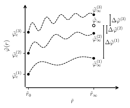
A system of ordinary differential equations (ODEs) can only be numerically solved as an initial value problem. In this case, initial conditions are given at the same point, e.g. $r=0$ , and evolved by integrating the ODE system using, e.g. a Runge-Kutta method. In our case, the boundary conditions are given at the center of the star, $r=r_{0}$ , and towards infinity, $r=r_{\infty}$ . Numerically speaking, $r_{0}$ and $r_{\infty}$ are small/large enough numbers respectively ³³ 3 ”Small/large enough” meaning that numerical results will not significantly change if these values are decreased/increased.. A shooting method reduces this problem to an initial value problem. For variables with a boundary condition at infinity, the method finds the initial value at the center that correctly leads to the given boundary value. These variables are called shooting parameters. For the system (14), the scalar field is the only relevant shooting parameter as the temporal metric function $\tilde{\phi}(\tilde{r})$ only enters the equations through its derivative and can thus be eliminated from the equations.

Here we outline the procedure for the scalar field $\tilde{\varphi}$ . A visualization is shown in Fig. 5. The method follows the following procedure:

1.

First, we set the target value of the scalar field at numerical infinity $\tilde{\varphi}_{\infty}$ and the score function

$\Delta\tilde{\varphi}:=\tilde{\varphi}_{\infty}-\tilde{\varphi}(\tilde{r}_{\infty})\,.$

The score function is a directional measure for how far off we are from our desired target value and $\Delta\tilde{\varphi}=0$ means that we exactly hit our target.
2.

The first iteration takes a random guess for the initial value of the scalar field $\tilde{\varphi}_{c}^{(1)}$ . We evolve our variables by integrating the differential equations with this guess and the remaining initial conditions. In this way, we find the value of the scalar field at infinity $\tilde{\varphi}_{\infty}^{(1)}$ and can compute the score function $\Delta\tilde{\varphi}^{(1)}$ .
3.

In the next step, the code slightly varies the first initial guess to define a second initial guess $\tilde{\varphi}_{c}^{(2)}$ . Again, the variables are evolved using the ODEs. We find $\tilde{\varphi}_{\infty}^{(2)}$ at infinity and can compute $\Delta\tilde{\varphi}^{(2)}$ . Let us assume that $\tilde{\varphi}_{c}^{(2)}>\tilde{\varphi}_{c}^{(1)}$ and $\mathrm{sgn}(\Delta\tilde{\varphi}^{(2)})=\mathrm{sgn}(\Delta\tilde{\varphi}^{(1)})$ . If $|\Delta\tilde{\varphi}^{(2)}|>|\Delta\tilde{\varphi}^{(1)}|$ , we are moving in the wrong direction. Our third guess should be smaller than $\tilde{\varphi}_{c}^{(1)}$ . If $|\Delta\tilde{\varphi}^{(2)}|<|\Delta\tilde{\varphi}^{(1)}|$ and $\Delta\tilde{\varphi}^{(2)}\neq 0$ , we are moving in the right direction, but still haven’t hit our target value. Let us assume the latter case and continue to a third guess.
4.

Our assumption in the last step means that our third guess should be larger than the previous ones, i.e. $\tilde{\varphi}_{c}^{(3)}>\tilde{\varphi}_{c}^{(2)}$ . Once more, we solve the system with this guess and compute the score function. Let us now assume that $\mathrm{sgn}(\Delta\tilde{\varphi}^{(3)})\neq\mathrm{sgn}(\Delta\tilde{\varphi}^{(2)})$ . This means that we are beyond our target value $\tilde{\varphi}_{\infty}$ , we overshooted. Hence, the desired initial value must lay between the second and third guess, i.e. $\tilde{\varphi}_{c}^{(3)}>\tilde{\varphi}_{c}>\tilde{\varphi}_{c}^{(2)}$ .
5.

By carrying on with this procedure, we can continue to narrow down the correct initial value for the scalar field $\tilde{\varphi}_{c}$ that hits the target value at infinity $\tilde{\varphi}_{\infty}$ . Note that numerically speaking, we will never arrive at $\Delta\tilde{\varphi}=0$ . Instead, we have to set the desired accuracy, e.g. $|\Delta\tilde{\varphi}|=10^{-10}$ . Once the score function goes below this value, we accept the result as “correct.”

References

Amendola et al. (2018) L. Amendola, J. Rubio, and C. Wetterich Primordial black holes from fifth forces. Phys. Rev. D 97, pp. 081302(R). External Links: Document, 1711.09915 Cited by: §1.
Anderson (1929) W. Anderson Über die Grenzdichte der Materie und der Energie. Zeitschrift für Physik 56 (11-12), pp. 851–856. External Links: Document Cited by: §1.
Astashenok et al. (2022) A. V. Astashenok, S. D. Odintsov, and V. K. Oikonomou Maximal masses of white dwarfs for polytropes in R ${}^{2}$ gravity and theoretical constraints. Phys. Rev. D 106 (12), pp. 124010. External Links: Document, 2209.13693 Cited by: §1.
Bachs-Esteban et al. (2025) J. Bachs-Esteban, I. Lopes, and J. Rubio Screening mechanisms on white dwarfs: symmetron and dilaton. Universe 11 (5), pp. 158. External Links: ISSN 2218-1997, Document, 2505.05871 Cited by: §3.2, §5.1, footnote 1.
Benvenuto et al. (1999) O. G. Benvenuto, L. G. Althaus, and D. F. Torres Evolution of white dwarfs as a probe of theories of gravitation: the case of Brans-Dicke. MNRAS 305 (4), pp. 905–919. External Links: Document Cited by: §1, §3.1.
Boshkayev et al. (2016) K. A. Boshkayev, J. A. Rueda, B. A. Zhami, Zh. A. Kalymova, and G. Sh. Balgymbekov Equilibrium structure of white dwarfs at finite temperatures. International Journal of Modern Physics: Conference Series 41, pp. 1660129. External Links: ISSN 2010-1945, Document, 1510.02024 Cited by: §1, §5.1.
Brans and Dicke (1961) C. Brans and R. H. Dicke Mach’s principle and a relativistic theory of gravitation. Phys. Rev. 124, pp. 925–935. External Links: Document Cited by: §1, §3.1, §3.
Brax et al. (2010) P. Brax, C. van de Bruck, A. Davis, and D. Shaw Dilaton and modified gravity. Phys. Rev. D 82, pp. 063519. External Links: Document, 1005.3735 Cited by: §3.2, §3.
Casas et al. (2016) S. Casas, V. Pettorino, and C. Wetterich Dynamics of neutrino lumps in growing neutrino quintessence. Phys. Rev. D 94, pp. 103518. External Links: Document, 1608.02358 Cited by: §1.
Chandrasekhar (1931) S. Chandrasekhar The Maximum Mass of Ideal White Dwarfs. ApJ 74, pp. 81. External Links: Document Cited by: §1, §2.
Choudhuri (2010) A. R. Choudhuri Astrophysics for physicists. Cambridge University Press. Cited by: §1.
Crisostomi et al. (2019) M. Crisostomi, M. Lewandowski, and F. Vernizzi Vainshtein regime in scalar-tensor gravity: Constraints on degenerate higher-order scalar-tensor theories. Phys. Rev. D 100 (2), pp. 024025. External Links: Document, 1903.11591 Cited by: §1.
Damour and Esposito-Farese (1992) T. Damour and G. Esposito-Farese Tensor multiscalar theories of gravitation. Class. Quant. Grav. 9, pp. 2093–2176. External Links: Document Cited by: §1, §3, §3.
Das and Mukhopadhyay (2015) U. Das and B. Mukhopadhyay Modified Einstein’s gravity as a possible missing link between sub- and super-Chandrasekhar type Ia supernovae. J. Cosmology Astropart. Phys 2015 (5), pp. 045–045. External Links: Document, 1411.1515 Cited by: §1.
Doneva et al. (2024) D. D. Doneva, F. M. Ramazanoǧlu, H. O. Silva, T. P. Sotiriou, and S. S. Yazadjiev Spontaneous scalarization. Reviews of Modern Physics 96 (1), pp. 015004. External Links: Document, 2211.01766 Cited by: §1, §3.1, §3.
Doneva et al. (2013) D. D. Doneva, S. S. Yazadjiev, N. Stergioulas, and K. D. Kokkotas Rapidly rotating neutron stars in scalar-tensor theories of gravity. Phys. Rev. D 88 (8), pp. 084060. External Links: 1309.0605, Document Cited by: §3.
Filippenko et al. (1992) A. V. Filippenko, M. W. Richmond, D. Branch, M. Gaskell, W. Herbst, C. H. Ford, R. R. Treffers, T. Matheson, L. C. Ho, A. Dey, W. L. W. Sargent, T. A. Small, and W. J. M. van Breugel The Subluminous, Spectroscopically Peculiar Type 1a Supernova 1991bg in the Elliptical Galaxy NGC 4374. AJ 104, pp. 1543. External Links: Document Cited by: §1.
Freire et al. (2012) P. C. C. Freire, N. Wex, G. Esposito-Farèse, J. P. W. Verbiest, M. Bailes, B. A. Jacoby, M. Kramer, I. H. Stairs, J. Antoniadis, and G. H. Janssen The relativistic pulsar-white dwarf binary PSR J1738+0333 - II. The most stringent test of scalar-tensor gravity. MNRAS 423 (4), pp. 3328–3343. External Links: Document, 1205.1450 Cited by: §1, §3.1, §3.1.
Goh et al. (2024) L. W. K. Goh, J. Bachs-Esteban, A. Gómez-Valent, V. Pettorino, and J. Rubio Observational constraints on early coupled quintessence. Phys. Rev. D 109, pp. 023530. External Links: Document, 2308.06406 Cited by: §1.
Hinterbichler et al. (2011) K. Hinterbichler, J. Khoury, A. Levy, and A. Matas Symmetron cosmology. Phys. Rev. D 84, pp. 103521. External Links: Document, 1107.2112 Cited by: §5.1.
Hinterbichler and Khoury (2010) K. Hinterbichler and J. Khoury Screening long-range forces through local symmetry restoration. Phys. Rev. Lett. 104, pp. 231301. External Links: Document, 1001.4525 Cited by: §3.2, §3.
Howell et al. (2006) D. A. Howell, M. Sullivan, P. E. Nugent, R. S. Ellis, A. J. Conley, D. Le Borgne, R. G. Carlberg, J. Guy, D. Balam, S. Basa, D. Fouchez, I. M. Hook, E. Y. Hsiao, J. D. Neill, R. Pain, K. M. Perrett, and C. J. Pritchet The type Ia supernova SNLS-03D3bb from a super-Chandrasekhar-mass white dwarf star. Nature 443 (7109), pp. 308–311. External Links: Document, astro-ph/0609616 Cited by: §1.
Jain et al. (2016) R. K. Jain, C. Kouvaris, and N. G. Nielsen White Dwarf Critical Tests for Modified Gravity. Phys. Rev. Lett. 116 (15), pp. 151103. External Links: Document, 1512.05946 Cited by: §1.
Järv et al. (2015) L. Järv, P. Kuusk, M. Saal, and O. Vilson Invariant quantities in the scalar-tensor theories of gravitation. Phys. Rev. D 91 (2), pp. 024041. External Links: 1411.1947, Document Cited by: §3.1, §3.
Kalita and Mukhopadhyay (2018) S. Kalita and B. Mukhopadhyay Modified Einstein’s gravity to probe the sub- and super-Chandrasekhar limiting mass white dwarfs: a new perspective to unify under- and over-luminous type Ia supernovae. J. Cosmology Astropart. Phys 2018 (9), pp. 007. External Links: Document, 1805.12550 Cited by: §1.
Kamiya et al. (2012) Y. Kamiya, M. Tanaka, K. Nomoto, S. I. Blinnikov, E. I. Sorokina, and T. Suzuki Super-Chandrasekhar-mass Light Curve Models for the Highly Luminous Type Ia Supernova 2009dc. ApJ 756 (2), pp. 191. External Links: Document, 1207.4648 Cited by: §1.
Lauffer et al. (2018) G. R. Lauffer, A. D. Romero, and S. O. Kepler New full evolutionary sequences of H- and He-atmosphere massive white dwarf stars using MESA. MNRAS 480 (2), pp. 1547–1562. External Links: Document, 1807.04774 Cited by: §1.
Lieb and Yau (1987) E. H. Lieb and H. Yau A Rigorous Examination of the Chandrasekhar Theory of Stellar Collapse. ApJ 323, pp. 140. External Links: Document Cited by: §1.
Littenberg and Yunes (2019) T. B. Littenberg and N. Yunes Binary white dwarfs as laboratories for extreme gravity with LISA. Classical and Quantum Gravity 36 (9), pp. 095017. External Links: Document, 1811.01093 Cited by: §1.
Nomoto et al. (1997) K. Nomoto, K. Iwamoto, and N. Kishimoto Type Ia supernovae: their origin and possible applications in cosmology.. Science 276, pp. 1378–1382. External Links: Document, astro-ph/9706007 Cited by: §1.
Olmo et al. (2020) G. J. Olmo, D. Rubiera-Garcia, and A. Wojnar Stellar structure models in modified theories of gravity: Lessons and challenges. Phys. Rept. 876, pp. 1–75. External Links: 1912.05202, Document Cited by: §1, §1, §3.1.
Panotopoulos and Lopes (2020) G. Panotopoulos and I. Lopes White dwarf cooling via gravity portals. Phys. Rev. D 101 (2), pp. 023017. External Links: Document, 2001.06004 Cited by: §1.
Perivolaropoulos (2010) L. Perivolaropoulos PPN Parameter gamma and Solar System Constraints of Massive Brans-Dicke Theories. Phys. Rev. D 81, pp. 047501. External Links: 0911.3401, Document Cited by: §3.1.
Ruiter and Seitenzahl (2025) A. J. Ruiter and I. R. Seitenzahl Type Ia supernova progenitors: a contemporary view of a long-standing puzzle. A&A Rev. 33 (1), pp. 1. External Links: Document, 2412.01766 Cited by: §1.
Saltas et al. (2018) I. D. Saltas, I. Sawicki, and I. Lopes White dwarfs and revelations. J. Cosmology Astropart. Phys 2018 (5), pp. 028. External Links: Document, 1803.00541 Cited by: §1.
Saridakis et al. (2021) E. N. Saridakis, R. Lazkoz, V. Salzano, P. V. Moniz, S. Capozziello, J. B. Jiménez, M. D. Laurentis, G. J. Olmo, Y. Akrami, S. Bahamonde, J. L. Blázquez-Salcedo, C. G. Böhmer, C. Bonvin, M. Bouhmadi-López, P. Brax, G. Calcagni, R. Casadio, J. A. R. Cembranos, Á. de la Cruz-Dombriz, A. Davis, A. Delhom, E. D. Valentino, K. F. Dialektopoulos, B. Elder, J. M. Ezquiaga, N. Frusciante, R. Garattini, L. Á. Gergely, A. Giusti, L. Heisenberg, M. Hohmann, D. Iosifidis, L. Kazantzidis, B. Kleihaus, T. S. Koivisto, J. Kunz, F. S. N. Lobo, M. Martinelli, P. Martín-Moruno, J. P. Mimoso, D. F. Mota, S. Peirone, L. Perivolaropoulos, V. Pettorino, C. Pfeifer, L. Pizzuti, D. Rubiera-Garcia, J. L. Said, M. Sakellariadou, I. D. Saltas, A. S. Mancini, N. Voicu, and A. Wojnar Modified Gravity and Cosmology. An Update by the CANTATA Network. Springer. External Links: 2105.12582, Document, ISBN 978-3-030-83714-3, 978-3-030-83717-4, 978-3-030-83715-0 Cited by: §1.
Sarmah et al. (2022) L. Sarmah, S. Kalita, and A. Wojnar Stability criterion for white dwarfs in Palatini f (R ) gravity. Phys. Rev. D 105 (2), pp. 024028. External Links: Document, 2111.08029 Cited by: §1.
Shapiro and Teukolsky (2008) S. L. Shapiro and S. A. Teukolsky Black Holes, White Dwarfs and Neutron Stars: The Physics of Compact Objects. Wiley. Cited by: §1.
Stoner (1930) E. Stoner The Equilibrium of Dense Stars. Philos. Mag. 9 (60), pp. 944–963. External Links: Document Cited by: §1.
Stritzinger et al. (2006) M. Stritzinger, P. A. Mazzali, J. Sollerman, and S. Benetti Consistent estimates of ${}^{56}$ Ni yields for type Ia supernovae. A&A 460 (3), pp. 793–798. External Links: Document, astro-ph/0609232 Cited by: §1.
Vidal et al. (2025) S. Vidal, A. Wojnar, L. Järv, and D. Doneva Crystallized white dwarf stars in scalar-tensor gravity. Phys. Rev. D 111, pp. 084075. External Links: Document, 2408.15937 Cited by: §3.2, §4.
Wetterich (2007) C. Wetterich Growing neutrinos and cosmological selection. Physics Letters B 655 (5), pp. 201–208. External Links: ISSN 0370-2693, Document, 0706.4427 Cited by: §1.
Will (2018) C. M. Will Theory and experiment in gravitational physics. 2 edition, Cambridge University Press. External Links: Document Cited by: §1.
Wojnar (2021) A. Wojnar White dwarf stars in modified gravity. International Journal of Geometric Methods in Modern Physics 18, pp. 2140006–60. External Links: Document, 2012.13927 Cited by: §1.