When Method Choice Changes Statistical Inference:
A Comparison of a Baseline Two-Stage Approach and Bayesian Joint
Modeling for Longitudinal and Survival Data in an HIV Clinical Trial
Abstract
The two-stage approach and Bayesian joint modeling are commonly used to analyze longitudinal biomarker measurements together with time-to-event outcomes. Using data from an HIV clinical trial of 467 patients with repeated CD4 measurements and all-cause mortality as the survival outcome, we compared a baseline two-stage approach with a Bayesian joint model. The two-stage analysis fitted a linear mixed-effects model and included each patient’s predicted baseline CD4 value as a fixed covariate in a Cox proportional hazards model. The joint model simultaneously modeled the longitudinal CD4 process and survival while linking mortality risk to the current underlying CD4 value. The estimated association between ddI and mortality was similar in direction and magnitude across the two approaches. The two-stage estimate was HR (95% CI: –), whereas the joint-model estimate was HR (95% CrI: –). The estimated protective association of CD4 was stronger under the joint model (HR ) than under the two-stage approach (HR ). Because the approaches used different summaries of the longitudinal CD4 process, the observed differences cannot be attributed solely to measurement error or informative dropout. The findings demonstrate that the treatment of longitudinal biomarker information can materially affect statistical inference.
Keywords: joint models; longitudinal data; survival analysis; Bayesian estimation; two-stage approach; HIV; CD4 cell count; MCMC
1 Introduction
In clinical and epidemiological research, repeated measurements of a biomarker are often collected together with a time-to-event outcome for the same individuals. Studies of HIV progression, cancer treatment, and chronic disease management routinely generate this type of joint longitudinal-survival data. Appropriate analysis is important because the biomarker process and the event process may be related, and inadequate treatment of that relationship can lead to biased or misleading estimates.
A common applied strategy is the two-stage approach. In the first stage, a linear mixed-effects model is fitted to the longitudinal biomarker data to obtain patient-specific predicted values. In the second stage, those predictions are included as covariates in a Cox proportional hazards model for the survival outcome.[1] Although intuitive and relatively easy to implement, this strategy has well-documented limitations.[2] In particular, it may treat estimated biomarker values as fixed and known, thereby failing to propagate uncertainty from the longitudinal model into the survival model. It may also inadequately address informative dropout when patients who experience the event earlier contribute fewer longitudinal measurements.[3]
Joint models address these issues by modeling the longitudinal and survival processes within a unified framework.[4] The longitudinal submodel characterizes the underlying biomarker trajectory, while the survival submodel links the instantaneous event hazard to a feature of that trajectory, such as its current value. Under appropriate model specification, this shared-parameter framework can account for measurement error in the biomarker process and dependence between longitudinal follow-up and the event process.[4, 5]
The theoretical basis for joint modeling is well established. Tsiatis et al. demonstrated that naive incorporation of longitudinal covariates into survival models can produce biased estimates when the covariate is measured with error.[3] Wulfsohn and Tsiatis proposed a foundational joint modeling framework that estimates the longitudinal and survival processes simultaneously.[4] Rizopoulos later provided a comprehensive treatment of joint models and accessible software implementations in R.[6]
Despite these developments, two-stage analyses remain common in applied work because they are familiar, easy to implement, and computationally convenient. Previous studies have compared two-stage and joint-modeling strategies theoretically and through simulation,[2, 3] but practical comparisons using accessible clinical datasets remain useful for illustrating how modeling choices affect interpretation.
This paper uses data from a randomized clinical trial comparing didanosine (ddI) and zalcitabine (ddC) in HIV-positive patients.[7] We compare a baseline two-stage approach with a Bayesian joint model for the relationship between repeated CD4 measurements and time to death. The purpose is not to claim that one method alone changes the underlying clinical effect. Rather, the study illustrates how alternative representations of longitudinal biomarker information can produce different inferential statements. The Bayesian joint model was fitted using the freely available JMbayes2 package in R.[8]
The remainder of the paper is organized as follows. Section 2 describes the data and statistical methods. Section 3 presents the results. Section 4 discusses their implications and limitations. Section 5 concludes.
2 Methods
2.1 Data
We used the AIDS clinical trial dataset available in the JMbayes2 package in R,[8] originally derived from a randomized controlled trial comparing didanosine (ddI) and zalcitabine (ddC) in HIV-positive patients.[7] The dataset included 467 patients followed for up to 21.4 months. The longitudinal outcome was the square root of CD4 cell count, measured at baseline and approximately every 6 months, yielding 1,405 observations. The number of CD4 measurements per patient ranged from 1 to 5, reflecting unbalanced follow-up due to dropout and early death. The survival outcome was time to death, with 188 deaths observed (40.3% event rate). Baseline covariates included drug assignment (ddI vs. ddC), prior opportunistic infection (AIDS vs. no AIDS), and prior AZT use (failure vs. intolerance).
2.2 Statistical Analysis
All analyses were conducted in R version 4.5 using nlme version 3.1-164 and JMbayes2 version 0.4-5.[9, 10, 8]
2.2.1 Baseline Two-Stage Approach
In the first stage, we fitted a linear mixed-effects model for the square-root-transformed CD4 trajectory. Fixed effects were included for observation time, drug assignment, prior opportunistic infection, and prior AZT use. Random intercepts and random slopes for time were included at the patient level:
| (1) |
where is the square root of the CD4 count for patient at time , are patient-specific random effects, and is the residual error.
In the second stage, a patient-specific predicted CD4 value was extracted at baseline and entered as a time-fixed covariate in a Cox proportional hazards model together with drug assignment, prior opportunistic infection, and prior AZT use:
| (2) |
where is the predicted baseline square-root CD4 value for patient from Stage 1 and is the unspecified baseline hazard.
This baseline two-stage approach treats the predicted baseline CD4 value as fixed and does not propagate uncertainty from the longitudinal model into the Cox model. It also differs from the joint model because it uses a single baseline summary rather than the evolving CD4 trajectory.
2.2.2 Bayesian Joint Model
We fitted a Bayesian joint model using the JMbayes2 package.[8] The model simultaneously estimated a linear mixed-effects submodel for CD4 and a survival submodel for time to death. The longitudinal submodel had the same form as Equation (1). The survival submodel was
| (3) |
where
| (4) |
is the current underlying square-root CD4 trajectory and is the association parameter linking the longitudinal and survival submodels. The joint model therefore relates mortality risk to the current underlying CD4 value rather than to a single predicted baseline value.
The two approaches do not use identical representations of the longitudinal exposure. Their estimates should therefore be interpreted as a practical comparison of two analysis strategies rather than as an isolated test of measurement-error correction.
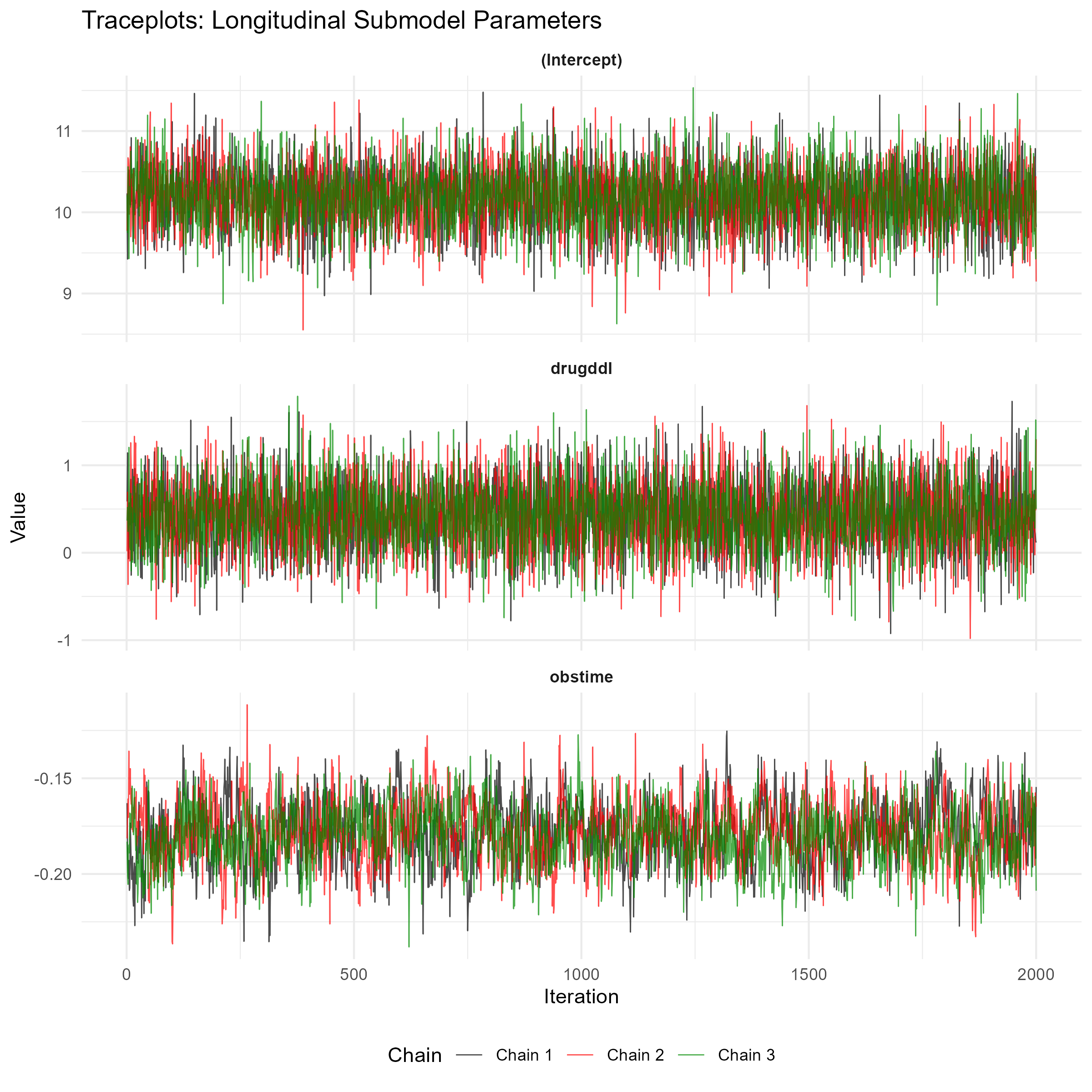
The model was estimated using Markov chain Monte Carlo sampling with three parallel chains, 12,000 iterations per chain, 2,000 burn-in iterations, and a thinning factor of 5. This yielded 2,000 retained posterior samples per chain. The default prior and baseline-hazard settings in JMbayes2 version 0.4-5 were retained. Convergence was assessed visually using traceplots and by Gelman–Rubin statistics, with all .[11]
2.3 Model Comparison
The approaches were compared with respect to four quantities: (1) the estimated association between CD4 and mortality, (2) the association between drug assignment and mortality, (3) the association between prior opportunistic infection and mortality, and (4) the association between prior AZT use and mortality.
For the two-stage approach, we report hazard ratios (HRs), 95% confidence intervals (CIs), and Wald-test -values. For the Bayesian joint model, we report posterior HRs and 95% credible intervals (CrIs). Because the two-stage model used predicted baseline CD4 and the joint model used the current underlying CD4 value, the corresponding CD4 HRs do not have identical interpretations.
3 Results
3.1 Data Description
The dataset comprised 467 HIV-positive patients followed for a median of 16.97 months (range: 0.5 to 21.4 months). A total of 1,405 CD4 measurements were recorded, with patients contributing between 1 and 5 observations. The overall event rate was 40.3%, with 188 deaths observed during follow-up. The study included 237 patients randomized to ddC and 230 randomized to ddI.
| Variable | Category/Statistic | Value |
|---|---|---|
| Survival outcome | ||
| Follow-up time (months) | Median (range) | 16.97 (0.5–21.4) |
| Deaths | (%) | 188 (40.3%) |
| Longitudinal outcome | ||
| CD4 measurements | Total | 1,405 |
| Measurements per patient | Range | 1–5 |
| CD4 count, square-root scale | Mean (SD) | 7.02 (3.91) |
| Baseline covariates | ||
| Drug assignment | ddC | 237 (50.7%) |
| ddI | 230 (49.3%) | |
| Prior opportunistic infection | AIDS | 232 (49.7%) |
| No AIDS | 235 (50.3%) | |
| Prior AZT use | Intolerance | 241 (51.6%) |
| Failure | 226 (48.4%) | |
3.2 Descriptive Analysis
Individual CD4 trajectories revealed substantial between-patient variability in both baseline levels and rates of change over time (Figure 1). Although the overall pattern suggested a decline in CD4 during follow-up, some patients showed stable or increasing trajectories, supporting the use of patient-specific random effects.

The descriptive mean CD4 trajectories by drug group are shown in Figure 2. The LOESS curves suggested that the groups may have differed in their average patterns over time. However, these curves are descriptive, and the fitted longitudinal model did not include a time-by-drug interaction.

Kaplan–Meier survival curves are shown in Figure 3. The unadjusted log-rank test did not identify a statistically significant difference between the drug groups ().

3.3 Baseline Two-Stage Approach
In Stage 1, square-root CD4 declined over time ( per month, ). Prior opportunistic infection was associated with a lower baseline square-root CD4 value (, ). Drug assignment was not associated with baseline square-root CD4 (), and prior AZT use was also not associated with baseline square-root CD4 (). Because the model did not include a time-by-drug interaction, it assumed the same average rate of CD4 change for both treatment groups.
In Stage 2, a higher predicted baseline square-root CD4 value was associated with a lower hazard of death (HR , 95% CI: –, ). After adjustment for predicted baseline CD4 and the other covariates, ddI was associated with a higher hazard of death than ddC (HR , 95% CI: –, ). Prior opportunistic infection was associated with a higher hazard of death (HR , 95% CI: –, ). Prior AZT failure was not statistically significant (HR , 95% CI: –, ). The model concordance statistic was 0.724.
3.4 Bayesian Joint Model
The Bayesian joint model showed adequate convergence across all three MCMC chains. Gelman–Rubin statistics were below 1.01 for all monitored parameters, and visual inspection of the traceplots in Figure 4 indicated good mixing and stationarity.
The longitudinal submodel estimated a decline in square-root CD4 over time (posterior mean , 95% CrI: to ). Prior opportunistic infection was associated with a lower baseline square-root CD4 value (posterior mean , 95% CrI: to ).
In the survival submodel, a higher current underlying square-root CD4 value was associated with a lower hazard of death. The posterior log-hazard coefficient was (95% CrI: to ), corresponding to an HR of 0.776 (95% CrI: –). Thus, each one-unit increase in the current underlying square-root CD4 value was associated with an estimated 22.4% lower hazard of death.
The posterior HR for ddI versus ddC was 1.383 (95% CrI: –). The posterior estimate suggested a higher hazard for ddI, although the credible interval included 1. Prior opportunistic infection was associated with a higher hazard of death (HR , 95% CrI: –). The credible interval for prior AZT failure included 1 (HR , 95% CrI: –).


3.5 Comparison of Methods
Table 2 and Figure 6 compare the estimates from the two approaches. The estimated association between drug assignment and mortality was similar in direction and magnitude: HR under the baseline two-stage approach and HR under the joint model. The principal difference concerned uncertainty. The two-stage confidence interval narrowly excluded 1, whereas the joint-model credible interval included 1.
The joint model produced a stronger estimated association between CD4 and mortality. However, the CD4 hazard ratios are not directly equivalent because the two-stage analysis used a predicted baseline CD4 value while the joint model used the current underlying CD4 value.
| Baseline Two-Stage | Bayesian Joint Model | ||||
|---|---|---|---|---|---|
| Parameter | HR | 95% CI | HR | 95% CrI | |
| CD4, square-root scale | 0.826 | 0.781–0.873 | 0.776 | 0.720–0.830 | |
| Drug, ddI vs. ddC | 1.342 | 1.006–1.789 | 0.045 | 1.383 | 0.952–2.010 |
| Prior OI, AIDS vs. no AIDS | 1.910 | 1.203–3.031 | 0.006 | 1.801 | 1.103–2.999 |
| AZT, failure vs. intolerance | 1.111 | 0.810–1.522 | 0.515 | 1.089 | 0.781–1.523 |
Note. The two-stage CD4 estimate represents a predicted baseline value, whereas the joint-model CD4 estimate represents the current underlying square-root CD4 value. The two CD4 hazard ratios therefore do not have identical interpretations. Confidence intervals and credible intervals also arise from different inferential frameworks.

4 Discussion
This study compared a baseline two-stage approach with a Bayesian joint model for repeated CD4 measurements and survival in an HIV clinical trial. The estimated association between ddI and mortality was similar in direction and magnitude across the two approaches, but the methods differed in their quantification of uncertainty. The two-stage confidence interval narrowly excluded 1, whereas the joint-model credible interval included 1. The result should therefore not be described as a reversal in the estimated drug association. Instead, it shows that different modeling approaches can produce different inferential statements even when their point estimates are similar — which is precisely the sense in which method choice changed statistical inference in this analysis: the conclusion about statistical significance, not the estimated effect, depended on the method.
The stronger CD4 association under the joint model is consistent with established concerns about treating estimated longitudinal values as known covariates.[3, 4] Nevertheless, the present comparison does not isolate the effect of measurement-error correction because the models used different representations of CD4. The baseline two-stage approach used a single predicted baseline value, whereas the joint model used the evolving underlying CD4 trajectory. A more direct comparison would use time-varying predicted CD4 values in the second-stage Cox model.
The descriptive LOESS curves suggested possible differences in average CD4 patterns between treatment groups. However, the longitudinal submodel did not include a time-by-drug interaction and therefore did not formally estimate treatment-specific slopes. The descriptive curves should not be used to explain the difference between the survival-model results without an additional interaction analysis.
The Bayesian implementation was computationally manageable in this application. All three chains showed adequate convergence according to the traceplots and Gelman–Rubin diagnostics. Joint modeling nevertheless requires careful attention to the longitudinal and survival submodels, the association structure, prior distributions, baseline-hazard specification, convergence diagnostics, and interpretation.
Several limitations should be emphasized. First, the two approaches did not use identical summaries of the longitudinal CD4 process. Consequently, differences between their results cannot be attributed exclusively to measurement error or informative dropout. Second, the longitudinal submodel did not include a time-by-drug interaction, so treatment-specific differences in CD4 slopes were not formally evaluated. Third, the dataset was relatively small, with 467 patients, and the findings may not generalize to other studies. Fourth, sensitivity analyses using alternative prior specifications were not conducted. Fifth, only a current-value association structure was considered. Alternative structures, such as the slope of the CD4 trajectory or cumulative CD4 exposure, may yield different results. Finally, a simulation study would provide a more controlled assessment of when and why the methods diverge.
Despite these limitations, the analysis provides a useful applied illustration. The way a longitudinal biomarker is summarized and linked to a survival outcome can materially affect statistical inference. Bayesian joint modeling offers a coherent framework for simultaneous analysis, but its appropriateness depends on the research question, target estimand, model assumptions, and diagnostic evidence.
5 Conclusion
The baseline two-stage approach and Bayesian joint model produced similar point estimates for the association between drug assignment and mortality but differed in their representation of uncertainty. The two-stage confidence interval narrowly excluded the null, whereas the joint-model credible interval included 1. The joint model also estimated a stronger association between the current underlying CD4 value and mortality.
Because the baseline two-stage analysis used a single predicted CD4 value while the joint model used the evolving underlying CD4 trajectory, the observed differences cannot be attributed solely to measurement error or informative dropout. Instead, the findings show that the way longitudinal biomarker information is represented can materially affect survival-model inference. Bayesian joint modeling provides a coherent framework for simultaneously analyzing longitudinal and time-to-event outcomes, but its use should be guided by the research question, target estimand, model assumptions, and appropriate diagnostic checks. Future work should compare the joint model with a time-varying two-stage analysis and examine alternative association structures and prior specifications.
Acknowledgements
Not applicable.
Funding
This research received no specific grant from any funding agency in the public, commercial, or not-for-profit sectors.
Declaration of Conflicting Interests
The author declares no conflicting interests with respect to the research, authorship, and publication of this article.
Ethical Approval
This study used a publicly available dataset distributed with the JMbayes2 R package. No participants were recruited and no primary data were collected for this analysis.
Availability of Data and Code
The dataset is available through the JMbayes2 R package.[8] Analysis code is available from the corresponding author upon reasonable request.
References
- [1] Cox DR. Regression models and life-tables. Journal of the Royal Statistical Society: Series B. 1972;34(2):187–220.
- [2] Prentice RL. Covariate measurement errors and parameter estimation in a failure time regression model. Biometrika. 1982;69(2):331–342.
- [3] Tsiatis AA, DeGruttola V, Wulfsohn MS. Modeling the relationship of survival to longitudinal data measured with error: applications to survival and CD4 counts in patients with AIDS. Journal of the American Statistical Association. 1995;90(429):27–37.
- [4] Wulfsohn MS, Tsiatis AA. A joint model for survival and longitudinal data measured with error. Biometrics. 1997;53(1):330–339.
- [5] Tsiatis AA, Davidian M. Joint modeling of longitudinal and time-to-event data: an overview. Statistica Sinica. 2004;14:809–834.
- [6] Rizopoulos D. Joint Models for Longitudinal and Time-to-Event Data: With Applications in R. Boca Raton, FL: Chapman & Hall/CRC; 2012.
- [7] Goldman AI, Carlin BP, Crane LR, Launer C, Korvick JA, Deyton L, Abrams DI. Response of CD4 lymphocytes and clinical consequences of treatment using ddI or ddC in patients with advanced HIV infection. Journal of Acquired Immune Deficiency Syndromes and Human Retrovirology. 1996;11(2):161–169.
- [8] Rizopoulos D. JMbayes2: Extended Joint Models for Longitudinal and Time-to-Event Data. R package version 0.4-5; 2023.
- [9] R Core Team. R: A Language and Environment for Statistical Computing. Vienna, Austria: R Foundation for Statistical Computing; 2025.
- [10] Pinheiro J, Bates D, R Core Team. nlme: Linear and Nonlinear Mixed Effects Models. R package version 3.1-164; 2023.
- [11] Gelman A, Rubin DB. Inference from iterative simulation using multiple sequences. Statistical Science. 1992;7(4):457–472.