Theory of Household Portfolio Choice: Pitfalls in Applications of the Collective Model
Abstract
A number of recent empirical papers rely on a collective model to analyze the portfolio choice of spouses, their heterogeneous risk preferences, and intra-household bargaining. I study applications of this model and highlight some important shortcomings. In its classic form, the model generates a counterintuitive result: an increase in the risk aversion of a household member can lead to an increase in household risk-taking. I offer a formal characterization of this pattern and link it to previous theoretical findings. I highlight further issues with applications of the collective approach to the portfolio choice problem in the contexts of bargaining and wealth inequality. I reconcile recent household finance papers with these findings and point to potential confusion in the literature. I emphasize existing alternatives that do not exhibit most of these issues, yet argue that there is a lack of a consistent and rigorous modeling approach.
1 Introduction
The household finance literature almost exclusively assumes that the household acts as a single decision-making unit. For example, research interested in the relationship between household characteristics and financial outcomes commonly uses education, age, or risk aversion of the “household head” as a proxy for household characteristics. This unitary approach only works if the household consists of a single member or if all members of the household have identical objectives.
This paper studies portfolio choice decisions or, more precisely, risk-taking decisions of households. It is common to study heterogeneity in the risky share, defined as the share of the portfolio invested in risky assets. The fundamental result of a unitary framework is that an increase in the risk aversion of an agent always leads to a decrease in risk-taking. For example, a canonical formula from 17, , suggests that the optimal risky share, , is inversely related to the risk aversion, .
However, a household may consist of more than one member and these members may differ in their preferences for risk and such a unitary model may not be suitable11 1 Partners may also have heterogeneous beliefs about the stock market or investment horizons, but this is not the focus of this paper.. A growing strand of empirical work acknowledges that partners may differ in their risk attitudes and studies portfolio choice with measures of risk aversion for each spouse. Empirical estimates using the Health and Retirement Study (HRS), for example, show that a majority of spouses indeed differ in their risk preferences (3; 14).
There are a number of reasons why one might be interested in using measures of individual risk aversion of both spouses. On the one hand, one might attempt to better explain the empirical variation in the risky shares or participation of married partners across time and in the cross-section (16; 23; 20). In particular, this can help explain changes in portfolio choice after transitions to retirement or death of a member and can motivate time-varying risk aversion (1). On the other hand, one might be interested in measuring gender inequality or asymmetry in influence over decision-making under uncertainty (13; 11; 7). This empirical household finance research often explicitly or implicitly relies on a collective approach whereby individual preferences are scaled by some Pareto weights and aggregated into a household objective.
This paper has two major goals. The first is to discuss alternative approaches of applying the collective framework to the household portfolio choice problem and emphasize the drawbacks of these applications. In particular, I present a non-monotonicity result: an increase in the risk aversion of a member may lead to an increase in the household risky share. To the best of my knowledge, this has not been previously pointed out. In addition, I discuss other issues with this framework related to its applications to contexts with heterogeneous wealth levels and bargaining. The second is to review the existing work on intra-household portfolio choice in light of these results, reconcile different approaches with each other, and point to the potential confusion in the recent literature.
Pioneered by 8 and 4 the collective modeling approach is widely used in economics (see 12 for a recent review of applications in a gender economics context)22 2 There are some alternative approaches not discussed here. For example, one might model exogenous changes in family structure (15). A less common approach to intra-household decision making is to rely on an information asymmetry framework (5).. For example, 16 uses a collective framework to study the consumption-saving behavior of married couples. A number of empirical papers studying portfolio choice also rely on this collective framework. However, there is a lack of a consistent and rigorous modeling approach.
As a preview and in order to provide further motivation, I demonstrate the main result with the following example. Assume a household consists of two partners and chooses between a risky alternative , that provides $1 worth of a public good with probability 0.9 and $60 worth of a public good with probability 0.1 and a safe alternative , that provides a certain $5 worth of a public good33 3 This gamble is taken from 2.. Assume both partners have a CRRA utility over consumption with preference parameters and and the household maximizes the sum of expected individual utilities. I assume that the risk aversion of the first member is fixed at , and vary the risk aversion of the second member. At low values of the risk aversion of the second member (say ), the household prefers the risky alternative. At a slightly higher value (say ), the household starts preferring the safe alternative. However, if one continues to increase the risk aversion of the second member (say ), the household will now prefer the risky alternative again44 4 Under , we get . Under , we get . Finally, under , we get .
This example demonstrates a rather puzzling result: increasing the risk aversion of a member can increase the risk-taking of the household. I refer to this internal inconsistency as non-monotonicity. This pattern is counterintuitive and implies that such a collective framework should not be used in a setting where one is interested in risk preference heterogeneity. For example, one immediate practical implication is an identification problem: for a given level of risk aversion of the first member, different levels of risk aversion of the second member may be consistent with the observed behavior of the household. In this paper, I place the counterintuitive results obtained in this example in a more general context. In particular, I generalize to a continuous-choice and continuous-risk setup and derive some precise propositions.
I show that the optimal household risky share can increase with the risk aversion of its member under a household objective that additively aggregates individual CARA or CRRA utilities that depend on consumption of a public good. I provide intuition for this result, offer a formal characterization of this pattern, and show that it occurs on a wide range of economically meaningful values of exogenous parameters. In addition, I relate this result to the earlier theoretical findings of 2 who study the random utility model (RUM) using a unitary framework. I discuss other aggregation methods and highlight which methods always obey the intuitive monotonicity property (i.e., optimal risky share of the household always decreasing with the risk aversion of its member).
I also discuss the properties of this framework related to Pareto weights and wealth sensitivity. In particular, I show that different modeling assumptions result in vastly different empirical estimates of these Pareto weights, often interpreted as bargaining power of spouses. Moreover, I show that while the individual CRRA solution does not, the household solution that additively aggregates individual utilities depends on the level of wealth. Finally, I show that for lower levels of wealth, the household closely mimics the preferences of the more risk averse member, and for slightly higher levels of wealth, the household closely mimics the preferences of the less risk averse member.
To the best of my knowledge, the existing literature has not highlighted the non-monotonicity of household’s risk-taking with respect to the risk aversion of individuals consuming a public good. I show that such monotonicity is sometimes falsely taken for granted (see, for example, 23). I discuss the model used in a recent study by 11 who obtain a monotonic solution, yet mistakenly claim that their approach can be micro-founded by a collective framework whereby individual utilities are aggregated additively. I further demonstrate a potential source of confusion: simplifications to the objective functions made in the unitary approach (e.g. dropping the constants or using a mean-variance utility instead of the CARA utility) may not be applicable in the collective framework. I discuss alternative modeling approaches used in the empirical literature, such as aggregation of individual utilities by product, and show that they do not exhibit some of the counterintuitive features discussed above.
This paper contributes to the existing literature on multiple fronts. First, it contributes to a broad understanding of household portfolio choice and participation (see 10; 6 for a general review of the portfolio choice and stock market participation literature and section 4.4 of 10 for a partial review of the intra-household finance literature). Second, it contributes to the understanding of applications of the collective approach to decision-making, intra-household bargaining, and gender asymmetry. There is a growing body of literature on risk-taking behavior concerning intra-household bargaining and gender inequality. Using U.S. data, 13 estimates gender asymmetry when it comes to financial risk-taking using a finance-profession indicator as a proxy for finance sophistication. 11 attempt to estimate asymmetry in decision-making using Australian survey data, which contain estimates of individual risk aversion of both spouses. In the context of a rural Chinese town, 7 discuss a promising experimental approach to estimating asymmetry, yet authors do not provide or discuss a relevant model.
The paper is organized as follows. Section 2 presents the setup of the problem and discusses alternative modeling approaches common in the literature. Section 3 discusses solutions of these models and derives the main results. Section 4 reconciles the findings with the existing literature and emphasizes some pitfalls. Section 5 concludes.
2 Setup
In this section, I precisely describe the simple framework at hand as well as highlight the alternative assumptions within this framework made by the existing literature.
The household consists of two individuals . I will refer to these individuals interchangeably as agents, members, spouses, and partners. The household first decides how to invest its initial endowment , then returns are realized, and all resulting wealth is consumed by the members. There is no labor income. Matching in the marriage market is left outside the scope of this framework, and risk preferences of the partners are taken as given. Partners are fully committed and must collectively decide on the portfolio allocation that maximizes some household objective.
There are two assets available in the market: a risk-free asset with a safe return and a risky asset with excess return . Unless explicitly stated otherwise, I assume . A potential disagreement in beliefs about the risky return distribution is also outside of the scope of this framework. Portfolio allocation is summarized by the choice of the risky share, , defined as the share of endowment invested in the risky asset. Hence, household-level consumption is
| (1) |
Note that,
| (2) |
There are two extreme assumptions that can be made about individual consumption. I focus on the approach whereby both members are assumed to consume a single public good: . This approach is taken by the existing portfolio choice literature studying intra-household dynamics (e.g. see 1; 23; 20)55 5 An alternative approach not discussed in this paper is to assume that each member consumes only some private good: (e.g. see 16)..
I consider the two most common specifications of the individual utility functions: CARA utility with absolute risk aversion :
| (3) |
CRRA utility with relative risk aversion :
| (4) |
The household objective is some aggregation of individual utilities. Let represent the Pareto weight of individual and assume . These weights capture the extent to which individual preferences are represented in the household’s objective. Since full commitment is assumed, they can be thought of as exogenous bargaining weights.
The most common approach is to aggregate individual expected utilities by a weighted sum (see, for example, 19; 16; 23; 11):
| (5) |
This approach is intuitive because by varying ’s one will span the whole set of Pareto-efficient outcomes (21). An alternative, however, is to aggregate by taking the expectation of a weighted product of individual utilities (see 1):
| (6) |
In the next section, I will consider both of these methods in turn. For the sake of completeness, I will also consider aggregation by the product of expected utilities: , as well as the Nash Bargaining approach.
3 Results
Before proceeding with the collective framework, it is useful to consider the traditional individual maximization problem, also referred to as the unitary framework. This yields an individually optimal risky share which can be thought of as a counterfactual risky share that would have been picked by partner if she had total control over decision-making and maximized her own utility.
| (7) |
3.1 Individual Risk Aversion and Portfolio Choice
In this subsection, I derive the main results on the relationship between the risk aversion of an individual member of a household and household’s portfolio choice. I demonstrate that unlike the unitary approach, the collective framework yields a counterintuitive result in this portfolio choice setting: the share of household’s portfolio invested in the risky asset may increase with a risk aversion of its member. I discuss different utility aggregation assumptions in turn, with a special focus on the case of aggregation by sum.
3.1.1 Sum of expected utilities
Let be a vector of all exogenous parameters of the model. Assume that the household maximizes the sum of expected utilities:
| (8) |
Proposition 1.
For both CARA and CRRA individual utilities, there exists such that solution to the household problem in (8) is a non-monotonic function of the risk aversion of a member.
Proof.
In the Appendix Section A. ∎
Figure 1 uses the two examples from the proof to illustrate the result. Optimal household risky share is plotted against individually optimal ones which serve as a reference.


As can be seen from the figure, the optimal household risky share initially decreases with the risk aversion of the second member but eventually starts sloping upwards even though the risk aversion continues to increase. Thus, monotonicity of the household risky share with respect to the risk aversion of a member cannot be guaranteed under collective approach whereby individual CARA or CRRA utilities are aggregated additively. Moreover, Figure 1 demonstrates that such counterintuitive result occurs under economically meaningful values of and individual risk aversion parameters. Section B of the Appendix shows that non-monotonicity arises under other values of exogenous variables including the distributional assumptions of the risky asset return. In particular, it also shows that household risk-taking can increase with the risk aversion of the spouse even if that spouse has a higher bargaining weight.
I now provide intuition for non-monotonicity result using the following Lemma. Let be the derivative of the individual expected utility of member at the optimal risky share with respect to the risky share:
| (9) |
Lemma 1.
Solution to the household problem in (8) is a monotonic function of the risk aversion of member if and only if is a monotonic function of the risk aversion of member under both CARA and CRRA individual utilities.
Proof.
In the Appendix Section A. ∎
Therefore, the non-monotonicity result of Proposition 1 is related to the derivative of the individual expected utility at the optimal risky share with respect to the risky share. If this derivative is a non-monotonic function of individual risk aversion, then the household risky share will be a non-monotonic function of the risk aversion of this individual. In other words, collective solution is decreasing in the risk aversion of the second member as long as in the case of CARA and in the case of CRRA.
To provide further intuition, I now return to the binary choice example provided in the introduction and highlight the parallels to the continuous choice set-up of this section. Let be the risky alternative and be the safe alternative. The household prefers the risky alternative whenever
| (10) |
Assume for a given level of risk aversion of the first member, there is a level of risk aversion of the second member, in the case of CARA and in the case of CRRA, such that the household prefers the risky alternative for any risk aversion of the second member below this level and prefers the safe alternative for some risk aversion of the second member just above this level. Then, the analog of the monotonicity concept under the continuous choice set-up would be maintaining the preference for the safe alternative as the risk aversion of the second member increases above this threshold level. For an increasing risk aversion of the second member, the household will never switch back to preferring the risky alternative if,
| (11) |
Note the equivalence between the above and the discussed above. Figure 2 plots for an example in which inequality in (11) is violated, resulting in non-monotonicity.
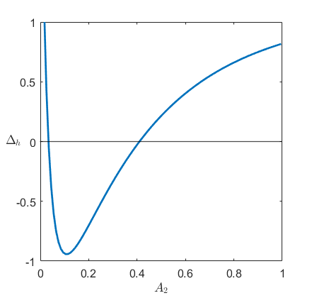
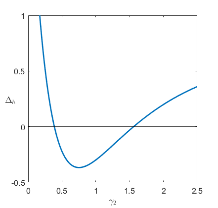
This demonstrates that non-monotonicity arises because increasing the risk aversion of a member may make them dislike the risky alternative less even though they still prefer the safe alternative. That is, the individual utility difference between the risky and safe gambles may be a non-monotonic function of the risk aversion of this individual. An analogous dynamic takes place in the continuous distribution of risk and continuous choice set-up: as agent 2 becomes more risk averse, she prefers a lower risky share but she also becomes more indifferent to similar risky shares, making the household objective more similar to the objective of agent 1.
The patterns in the binary choice example are directly related to the findings of 2. The authors study the random utility model (RUM) under the unitary framework and show that the RUM can be a non-monotonic function of the risk aversion. However, in part 1 of Proposition 1, the authors show that monotonicity of RUM is directly related to the monotonicity of which, as I have argued above, is in turn directly related to the monotonicity of the household-level decision66 6 In the language 2, and are not -ordered in my model..
An observation that can be made from Figure 1, is that the optimal risky share of the household is always between the two individually optimal counterfactual risky shares. The following Lemma shows that this is indeed always true under CARA preferences.
Lemma 2.
Let and assume for . Then, under CARA utility, when , and when .
Proof.
In the Appendix Section A. ∎
Note that when , the household problem reduces to the trivial individual problem and . The following proposition specifies conditions under which monotonicity can be guaranteed under CARA preferences.

Proposition 2.
Solution to the household problem in (8) is always a decreasing function of under CARA utility functions when and .
Proof.
In the Appendix Section A. ∎
So, under CARA preferences, the household risky share always decreases with the risk aversion of the less risk averse member. In Figure 1, this corresponds to the region to the left of the point where all three curves intersect. There is, however, no equivalent result under CRRA individual utilities: Figure 3 plots an example where household risky share increases with the risk aversion of the less risk averse member.


Finally, one might notice the somewhat arbitrary choice of the wealth level in the example given in Figure 1. This is because under , one always obtains monotonic household risky share under CRRA preferences. The following proposition shows formally that this is always true.
Proposition 3.
Solution to the household problem in (8) is a strictly decreasing function of the risk aversion of member under CRRA utility function when , and .
Proof.
In the Appendix Section A. ∎
The intuition for Proposition 3 can be obtained by noting that the marginal CRRA individual utility of consumption at is equal to 1 and is independent of the risk aversion parameter. Additional discussion in Appendix C elaborates on this point based on a wealth splitting example. Under a CARA individual utility function however, there is no level of consumption that would make the marginal utility independent of the risk aversion. Figure 4 demonstrates that even for lower levels of wealth, one can find risk aversion levels such that non-monotonicity is obtained under CARA preferences.
3.1.2 Expected product of utilities
Assume the household maximizes the expected product of utilities77 7 Due to the fact that utilities might be negative, in practice, we multiply them by -1 and minimize the objective instead of maximizing it.:
| (12) |
Proposition 4.
Solution to the household problem in (12) is always a monotonic function of the risk aversion of a member under both CARA and CRRA individual utilities.
Proof.
In the Appendix Section A. ∎
Multiplying individual CARA or CRRA utilities yields a household objective equivalent to the respective individual ones. This not only allows one to derive analytic solutions, but also guarantees monotonicity. Under CARA preferences, one obtains:
| (13) |
Under CRRA preferences and log-normal risky asset return, one obtains:
| (14) |
Observe that under both CARA and CRRA, optimal household risky share is a weighted harmonic average of individually optimal risky shares (i.e. ). Figure 5 visualizes the solution to the objective in (12) along with the solutions to the corresponding individual problems.


Note that even under equal bargaining weights, the household risky share is always closer to the smaller individual risky share. This will be the case under other parameters of the model as it stems directly from the properties of the harmonic average. I return to this solution in Section 3.2 when discussing identification of the bargaining weights and sensitivity of the solution to the wealth level.
3.1.3 Other approaches
In this subsection, I focus mostly on CARA individual utilities. Assume the household maximizes a weighted product of expected CARA utilities:
| (15) |
Proposition 5.
There exists such that solution to the household problem in (15) is a non-monotonic function of the risk aversion of a member.
Proof.
In the Appendix Section A. ∎
Assuming , the condition for monotonicity with respect to can be written as, . Since , monotonicity is guaranteed when . Note that this is in contrast to the result under sum of expected utilities where we can guarantee monotonicity with respect to when .
Motivated by 11, I also consider the Mean-Variance utility which is a monotonic transformation of the CARA utility:
Assume household maximizes weighted sum of individual Mean-Variance utilities. That is the household problem is:
| (16) |
Proposition 6.
Maximizing weighted sum of Mean-Variance utilities is equivalent to maximizing weighted product of expected CARA utilities.
Proof.
In the Appendix Section A. ∎
This equivalence can be observed by taking the logarithm of the objective function in (15) and comparing it to the objective in (16). Proposition 6 demonstrates that while under normally distributed risky return maximizing Mean-Variance utility is equivalent to maximizing expected CARA utility under the unitary framework, this is not the case under the collective framework. Now, redefine the objective in (16) slightly such that the household maximizes weighted sum of individual simplified Mean-Variance utilities (as in Gu et al., 2024) where the risk aversion parameter has been canceled out:
The household problem is:
| (17) |
Proposition 7.
Maximizing weighted sum of simplified Mean-Variance utilities is equivalent to maximizing expectation of a weighted product of CARA utilities.
Proof.
In the Appendix Section A. ∎
Proposition 7 demonstrates that while under the unitary framework maximizing Mean-Variance utility is equivalent to maximizing the simplified Mean-Variance utility, it is not the case under the collective framework.
Finally, consider the Nash Bargaining problem:
| (18) |
The following proposition shows that a Nash Bargaining solution can also be a non-monotonic function of the risk aversion of a member.
Proposition 8.
There exists and such that solution to the household problem in (18) is a non-monotonic function of the risk aversion of a member.
Proof.
In the Appendix Section A. ∎
3.2 Bargaining, Wealth, and Household Portfolio Choice
In this section, I discuss the role played by the Pareto weights and the wealth level in the household portfolio choice, and highlight further concerns with applications of the collective framework. First, I show that the inference about the Pareto weights in an empirical study is very sensitive to the assumptions of the collective decision-making framework. When it comes to the level of household wealth, I show that while it has no effect on the portfolio choice in the unitary framework under CRRA preferences, such independence breaks in a collective framework. Finally, I discuss issues of this framework related to the mutual identification of Pareto weights and the level of wealth.
3.2.1 Pareto Weights
As discussed in Section 2, it is common to think of the Pareto weights as coefficients summarizing the intra-household bargaining: for example, a greater is commonly interpreted as a greater ability of person to represent their preferences or influence the joint decisions. It is straightforward to show that all of the models discussed in Section 3 obey the following intuitive property: an increase in the bargaining power () of the more (less) risk averse spouse decreases (increases) the risky share of the household (for example, see 23 for a proof under the sum of expected utilities approach). However, I argue that different assumptions of the model result in vastly different estimates of Pareto weights for a given observation of household risky share and individual risk aversion levels.
Figure 6 plots optimal household and individual risky shares against the Pareto weight of the first individual (). Since the first member is assumed to be the less risk averse one, the household risky share always increases with the Pareto weight of the first member under both CARA and CRRA preferences.
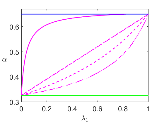
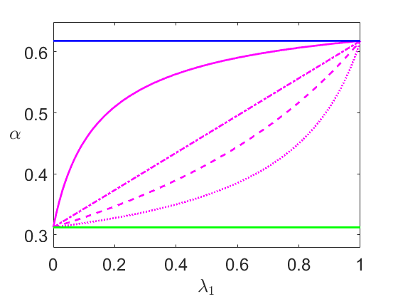
However, it is evident from Figure 6 that different aggregation methods result in vastly different patterns. Figure 7 plots a Pareto weight that would be required to fit an observed household risky share that is exactly between the two individually optimal ones (i.e. ). Under CARA (CRRA), required Pareto weight of the first individual varies from 0.04 (0.12) to 0.8 (0.83) for the sum of expected utilities and expectation of product of utilities respectively.
One alternative approach to the collective models discussed in Section 3.1 is to simply assume that the household risky share is the weighted average of the individually optimal risky shares where the weights reflect the individual bargaining power (i.e. ). Section 4 argues that the specification of 11 is equivalent to this approach. Given the specification imposed by the authors, Pareto weights reflect the distance between the household and individual optimal risky shares linearly. This will always result in an arguably intuitive Pareto weight of 0.5 when the household risky share is the average of the two individually optimal ones as in Figure 7. Note, however, that such linear relationship would not be maintained if one averages the risk aversion parameters instead of averaging the risky shares directly.88 8 This is because optimal risky share depends inversely on the risk aversion.


3.2.2 Wealth Level


While the individual CRRA solution is always independent of the wealth level, the collective solution using sum of expected CRRA utilities (see Section 3.1.1) is not. Figure 8 plots the optimal risky share (risky investment amount for CARA) against the level of wealth for both CARA and CRRA individual utilities. The optimal risk-taking increases with the wealth level99 9 The paper by 18 shows that the risk-taking increases with the wealth level of the household in a similar collaborative framework (Proposition 1). However, the wealth sensitivity of the risky share highlighted here is distinct from the one discussed by the authors. This is due to the fact that the results in 18 rely on an arbitrary parameter which essentially rescales the Pareto weight (and hence the marginal utility) of the second member (higher delta means lower weight placed on the utility of the second member). This is reverse engineered such that for a given level of wealth . Hence, depends on the wealth level and the difference in risk aversion parameters. For example, under equal Pareto weights, when the second member is the more risk averse one, higher wealth would require a lower which would make the solutions more similar to the individual solution of the second member. I note that, this approach is not micro-founded and in some sense monotonicity is artificially enforced. Authors do not show what happens to the household solution when is fixed.. More importantly, under both CARA and CRRA, as wealth levels increase (decrease), household-level solution converges to the individual solution of the less (more) risk averse individual. Under reasonable model parametrization and CRRA preferences, for a sufficiently high wealth level, the household solution closely resembles the solution of the less risk averse individual even using a very low Pareto weight for that individual (). Similarly, for a sufficiently low wealth level, the household solution closely resembles the solution of the more risk averse individual even using a very low Pareto weight for that individual (). This abrupt switching pattern makes application of a collective decision making framework whereby individual utility functions are aggregated additively, problematic in the context of portfolio choice and heterogeneous household wealth. As discussed in Section 3.1.2, however, the solution is independent of the wealth level under expected product of CRRA utilities.
Another relevant concern is related to the mutual identification of the wealth level and the Pareto weights of individuals. As can be seen from Figure 8, more than one combination of and can produce the same optimal risky share . This is not an issue if one observes either the wealth level of the household or the bargaining weights of individual members and is willing to use it directly in the model. If, however, both are unobserved, then the model will be unable to pin down both the wealth level and the Pareto weights.
4 Literature Implications
In this section, I review the existing literature in light of the findings of Section 3 and provide a reconciliation with some of the counterintuitive results. In all of the papers discussed here, household makes a decision under uncertainty by aggregating heterogeneous individual preferences of its members in one way or another.
11 is a recent empirical work interested in bargaining asymmetry in household portfolio choice decisions. Using Australian survey data, authors structurally estimate bargaining weights and find a large gender gap: “in an average household, the husband’s bargaining power is 60%, whereas the wife’s is 40%”. The authors also discuss gender and non-gender based determinants of this gap.
In order to estimate these bargaining weights, authors rely on the same setup as the one described in Section 2. In particular their setup is also static, with full spousal commitment and consumption of a single public good. Authors assume CARA individual utilities and normal distribution of shocks. Despite the fact that authors allow for participation costs, these costs can be set to zero in order to reconcile their approach with the results of Section 3. In 11, authors assume the household first aggregates risk aversion preferences of its members and then solves the standard individual maximization problem. Using my notation, this results in the following risky share solution.
| (19) |
This household solution is monotonically decreasing in the individual risk aversion levels. Surprisingly, however, authors claim that their modeling approach is equivalent to an approach whereby the household maximizes individual expected utilities aggregated additively:
Under the conditions detailed in Section B of the Internet Appendix, this gives an equivalent expression as in the classical collective bargaining model in which the household utility function is a weighted average of the individual’s utility (Manser and Brown 1980; McElroy and Horney 1981; Chiappori 1988a, 1992). Therefore, in our model, aggregating individual risk preferences is equivalent to aggregating individual utility functions.
In Section 3, I have shown that aggregating individual CARA utilities by a weighted average results in a non-monotonic solution which contradicts the equivalence claim made by 11. In section 3.1.3, I show that using Mean-Variance or simplified Mean-Variance individual utility functions also results in solutions different from the one obtained by the authors. Indeed, this equivalence claim is not accurate. Authors’ argument in Section B of the Internet Appendix essentially amounts to showing that under certain assumptions (in particular when ):
| (20) |
This, however, does not imply:
| (21) |
Despite the fact that the authors’ approach is not motivated by the classical theory of collective bargaining, it should be noted that the solution in equation (19) is intuitively appealing. For example, it can be motivated by an argument that the household chooses a weighted average of the two individually optimal risky shares (i.e., ). It is also the same as the risky share obtained by first splitting the wealth according to the bargaining weights, investing it separately as dictated by individual preferences, and then combining it back.
Finally, in Section 3.2, we have seen that using a different aggregation method would lead to a different estimate of bargaining weights. Hence, it is natural to ask how the estimates in 11 would change if a different specification is used.
Another empirical work on intra-household portfolio choices is a paper by 23 which uses the HRS data. The authors do not impose functional form assumptions on the individual utility functions yet rely on the same framework. In particular, it is assumed that household maximizes the weighted sum of expectations. The authors claim that their model predicts that the risky share will increase as the risk aversion of a spouse decreases.
One testable hypothesis derived from the theoretical framework is that the household invests a larger proportion of its wealth in risky assets when the spouse with more bargaining power is more risk tolerant.
However, this claim is not supported by the theoretical framework used in the paper and it is inaccurate. For example, we have seen in Section 3 that for both CARA and CRRA individual utility functions the household can decrease its investments in the risky asset when one of the spouses gets more risk tolerant (less risk averse), even when that spouse has greater bargaining power. This demonstrates that monotonicity might have been previously falsely taken for granted in the literature.
20 study participation, risky share and diversification decisions using administrative data from Sweden. The authors show empirically that an increase in female bargaining power (who are more risk averse on average) results in household taking less risk. The authors rely on a similar theoretical framework with full spousal commitment and consumption of a single public good. In their model, authors have two periods of consumption and the shocks have a binary distribution. The household is assumed to maximize a sum of expected CRRA utilities. Since authors do not directly utilize the model in their empirical analysis the solution to the household problem is not discussed in the main text. In particular, non-monotonicity implicit in their framework is not acknowledged.
A paper by 1 studies the portfolio choice of married couples in HRS as they transition into retirement. The author explicitly acknowledges that preferences can be heterogeneous and that the bargaining power may shift. The author uses a similar framework except there are three periods of consumption. Individuals are assumed to have CRRA preferences and the shocks follow a log-normal distribution. In contrast to the other papers, the author assumes that the household maximizes the expectation of product of the individual utility functions. As I show in Section 3.1.2, risk aversion of the household will then be a weighted average of the two risk aversions (i.e., always monotonic). Hence, in such a model the risky share of the household will be a weighted harmonic average of the individual risky shares. As discussed in Section 3.2, this means that the household risky share is always closer to the risky share of the spouse with the higher risk aversion which would require an asymmetric bargaining weight to fit a symmetric portfolio choice.
Finally, a paper by 16 is an influential paper interested in the precautionary savings behavior of couples with heterogeneous risk aversion and prudence. Unlike in the framework described in Section 2, the author assumes that the household can only invest in a risk-free asset and each spouse separately consumes their own private good. The uncertainty in the model comes only from the stochastic labor income and saving less implies taking more risk. Author obtains the following unexpected theoretical result: household savings can decrease when one spouse becomes more risk averse. My paper complements this work by showing that this counterintuitive result can be obtained with the public consumption assumption. In addition, 16 proves a theorem on non-monotonicity: increasing the risk aversion of the less risk averse member can increase the risk tolerance of the household. This is in contrast to my proposition 2 which shows that increasing the risk aversion of the less risk averse member can only decrease the risky share of the household.
5 Conclusion
In this paper, I analyze applications of the collective model to the household portfolio choice problem and highlight major shortcomings. In particular, I show that household risk-taking may increase when one of the spouses gets more risk averse1010 10 Despite the fact that household formation is not studied in the current theoretical framework, it can be argued that perfect matching on risk preferences cannot be guaranteed if risk aversion is heterogeneous across genders in aggregate.. Since household risk-taking also decreases with the risk aversion of the spouse, I refer to this pattern as non-monotonicity. I provide some precise characterization of this phenomenon and demonstrate that it occurs on economically meaningful levels of exogenous variables. In addition, I demonstrate that irrespective of the bargaining weights, for lower levels of wealth, the household closely mimics the more risk averse member and for slightly higher levels of wealth the household closely mimics the less risk averse member. These issues pose a major challenge for applications of the collective approach to the portfolio choice problem.
I review the recent empirical literature which has explicitly or implicitly relied on the given approach to study intra-household financial risk-taking and highlight some potential confusion. A recent paper by 11 proposes a preference aggregation approach which results in a solution free of the non-monotonicity problem. The authors, however, falsely claim that this approach is equivalent to the classical collective bargaining model. It should be noted that while the proposed solution in 11 seems like an intuitive one to use1111 11 I show that the approach in 11 is equivalent to choosing a risky share based directly on a weighted average of the individually optimal risky shares. For another example see 9 whereby instead of relying on a collective decision making approach, the outcome variable itself is aggregated by weighted averaging the counterfactual outcome variables. This solution also spans the whole range of Pareto efficient risky shares. In the current context full private consumption assumption could also justify this solution (22)., it is not micro-founded. In 1, the household aggregates individual utilities by first taking their product and then the expectation. In this case, household solution behaves intuitively when it comes to monotonicity and wealth sensitivity. However, I argue that such an approach has its own shortcomings as it requires asymmetric bargaining weights in order to fit an arguably fair household allocation.
Future empirical research interested in intra-household decision-making under uncertainty and estimation of the gender asymmetry in bargaining requires an alternative modeling approach. This approach should achieve desired theoretical properties not merely by relying on an alternative consumption specification or other assumptions of the collective model, but by appropriate fundamental characterization of the problem.
References
- Household portfolio choice and retirement. Review of Economics and Statistics 99 (5), pp. 870–883. Cited by: §1, §2, §2, §4, §5.
- Monotone stochastic choice models: the case of risk and time preferences. Journal of Political Economy 126 (1), pp. 74–106. Cited by: §1, Figure 2, Figure 2, §3.1.1, footnote 3, footnote 6.
- Preference parameters and behavioral heterogeneity: an experimental approach in the health and retirement study. The Quarterly Journal of Economics 112 (2), pp. 537–579. Cited by: §1.
- Efficient intra-household allocations: a general characterization and empirical tests. Econometrica, pp. 1241–1278. Cited by: §1.
- The good wife? reputation dynamics and financial decision-making inside the household. American Economic Review 115 (2), pp. 525–570. Cited by: footnote 2.
- Household finance in retrospect and prospect. Technical report National Bureau of Economic Research. Cited by: §1.
- The influence of spouses on household decision making under risk: an experiment in rural china. Experimental Economics 16 (3), pp. 383–401. Cited by: §1, §1.
- Rational household labor supply. Econometrica: Journal of the Econometric Society, pp. 63–90. Cited by: §1.
- Spousal influence and assortative mating on time preferences: a field experiment in the usa. Review of Economics of the Household 18 (2), pp. 461–512. Cited by: footnote 11.
- Household finance. Journal of Economic Literature 59 (3), pp. 919–1000. Cited by: §1.
- The gender gap in household bargaining power: a revealed-preference approach. The Review of Financial Studies, pp. hhae039. Cited by: §1, §1, §1, §2, Figure 6, §3.1.3, §3.2.1, §4, §4, §4, §4, §5, footnote 11, footnote 12.
- Women’s power in the household. Technical report National Bureau of Economic Research. Cited by: §1.
- Who wears the pants? gender identity norms and intrahousehold financial decision-making. The Journal of Finance 76 (3), pp. 1389–1425. Cited by: §1, §1.
- Imputing risk tolerance from survey responses. Journal of the American Statistical Association 103 (483), pp. 1028–1038. Cited by: §1.
- The effects of marital status and children on savings and portfolio choice. The Review of Financial Studies 23 (1), pp. 385–432. Cited by: footnote 2.
- Saving, risk sharing, and preferences for risk. American Economic Review 94 (4), pp. 1169–1182. Cited by: §1, §1, §2, §4, footnote 5.
- Lifetime portfolio selection under uncertainty: the continuous-time case. The Review of Economics and Statistics, pp. 247–257. Cited by: §1.
- Portfolio choice in a two-person household. Federal Reserve Bank of Richmond and University of Illinois at Urbana-Champaign working paper. Cited by: footnote 9.
- Risk attitudes and conflict in the household. The Economic Journal 132 (642), pp. 767–795. Cited by: §2.
- Bargaining over risk. Revise & Resubmit at the Review of Finance. Cited by: §1, §2, §4.
- Collective household models: principles and main results. Journal of Economic Surveys 16 (4), pp. 533–564. Cited by: §2.
- The theory of syndicates. Econometrica: Journal of the Econometric Society, pp. 119–132. Cited by: footnote 11.
- Portfolio choice and risk attitudes: a household bargaining approach. Review of Economics of the Household 13 (2), pp. 219–241. Cited by: §1, §1, §2, §2, §3.2.1, §4.
Appendix
A Proofs of Propositions and Lemmas
Proposition 1
Proof.
I prove the proposition by providing an example for each individual utility specification. Let us start with the case of CARA. Here, individual utility function can be written as,
| (22) |
Hence, because for any , we have , individual expected utility can be written as1212 12 Which only under unitary framework is equivalent to: . This is related to the issues with 11.,
| (24) |
There is no closed form solution to equation (24) but it can be solved for numerically. Figure 1, Panel A demonstrates one such solution where is a non-monotonic function of .
Let us now consider the case of CRRA. Here, individual utility can be written as,
| (25) |
and the individual expected utility can be written as,
| (26) |
Unlike in the case of CARA, there is no equivalent expression for the objective in (8) or the F.O.C. which does not include an expectation operator. One can solve for directly using a Monte-Carlo simulation. Figure 1, Panel B demonstrates one such solution where is a non-monotonic function of .
Since we found an example for both CARA and CRRA where is a non-monotonic function of the risk aversion of a member we have completed the proof.∎
Lemma 1
Proof.
Using the implicit function theorem one can write:
| (27) |
where is the household objective function evaluated at the solution and . The denominator of the RHS of equation (27) can thus be written as:
| (28) |
Since the S.O.C. of the individual maximization problem is always satisfied, both terms of the RHS of equation (28) are negative under CARA and CRRA. Hence, the sign of the LHS is the same as the sign of the numerator which is equal to ∎
Below, I show the S.O.C. for the CARA utility function as an example (the arguments are analogous for the CRRA utility function). Dropping the star superscript from the optimal :
| (29) |
Lemma 2
Proof.
Note that, since exponents are always positive, one of the following must be true for the F.O.C. in equation (24) to hold:
In the first case, we get . In the second case, we get and in the third case we get . ∎
Proposition 2
Proof.
Without loss of generality, assume . Given Lemma 1, we need to show that
| (30) |
Note that by Lemma 2, when we have since for . Hence, one can rewrite the condition as,
| (31) |
This inequality always holds due to Lemma 2 as for all (as ) and for all (as )1313 13 Note that the second term of the LHS in the inequality above is 0 in the individual case when . So the inequality always holds in the individual case for . .∎
Proposition 3
Proof.
Given Lemma 1, we need to show that . Given the definition in equation (26), individual expected utility under CRRA can be written as:
| (32) |
Then, one can write:
| (33) |
Set . We can then write,
| (34) |
Let . Hence, and we can rewrite the above equality as
| (35) |
Since the term is strictly positive for all non-zero , we obtain . ∎
Proposition 4
Proof.
First, assume the household maximizes the expected product of CARA utilities. The objective can then be written as
| (36) |
This is equivalent to the individual CARA maximization problem with a renamed coefficient of risk aversion (let ), solution to which is always decreasing in the risk aversion.
The same arguments can be used in the case of CRRA utilities. Assume the household maximizes the expected product of CRRA utilities. The objective can then be written as
| (37) |
This is equivalent to the individual CRRA maximization problem with a renamed coefficient of risk aversion (let ), solution to which is always decreasing in the risk aversion. ∎
Proposition 5
Proof.
The objective can be written as:
| (38) |
Applying the property of exponents we get:
| (39) |
The F.O.C. of (39) is (the denominator can be ignored as it does not depend on ):
| (40) |
Since the first term in the multiplication above is always positive, the second term has to be equal to 0. Hence, we obtain:
| (41) |
The solution is decreasing in if and only if:
| (42) |
This inequality does not hold for all . ∎
Proposition 6
Proposition 7
Proposition 8
Proof.

The objective is:
| (47) |
Despite the fact that the F.O.C. is analytical, there is no closed form solution for . Figure 10 visualizes a solution to an example which proves the proposition. ∎
B Alternative Parametrization of the Classic Collective Approach
Examples below illustrate that non-monotonicity arises under model parametrization different from the one considered in Section 3. Figure 11 plots the optimal risky shares assuming uniformly distributed risky asset return.


Figure 12 plots the optimal risky shares for alternative levels of bargaining weights and risk aversion.


C Wealth Splitting Problem
Assume full private consumption . Household decides how to split wealth between the two members in order maximize the sum of expected utilities. Let and .
| (48) |
The F.O.C. is:
| (49) |
That is, the marginal utilities weighted by the bargaining weights have to be equal. Observe that the risk aversion of a member affects the optimal split even though there is no uncertainty in this framework. At a sufficiently high (low) wealth level, the share allocated to person decreases (increases) with her risk aversion . Now, rewrite the F.O.C. as:
| (50) |
In order to eliminate and from the optimality condition, one needs to set . This requires and . When wealth equals 2, each member gets 1 unit of consumption and the optimal wealth split does not depend on their risk aversions. This is because at the marginal utility of consumption does not depend on the risk aversion . There is no equivalent statement for CARA as marginal CARA utility is and it always depends on the absolute risk aversion.