ReRound: Reconstructive Rounding to Resolve Midpoint Ambiguity
in Calibration-Free LLM Quantization
Abstract
ReRound (Reconstructive Rounding) is a post-training quantization method that addresses the midpoint ambiguity inherent in standard round-to-nearest (RTN) schemes when quantizing weights near the centers of quantization intervals.
Starting from a pretrained LLM, ReRound trains a conditional diffusion model to produce continuous reconstructions of low-bit weights for the LLM. These reconstructed weights act as a guidance signal to disambiguate the rounding direction of weights located close to interval midpoints.
To integrate this reconstruction-guided rounding with conventional RTN, ReRound introduces a tolerance metric measuring how far the quantized weight (not the final quantized integer) is away from the midpoint: quantized weights within a tolerance region around midpoints are quantized using diffusion-based reconstructions, whereas weights closer to quantization boundaries are quantized with RTN. By sweeping the tolerance parameter, ReRound generates multiple candidate quantized integer weight matrices and selects the de-quantized weight matrix candidate whose leading singular values most closely match those of the original full-precision weights. This selected candidate determines the tolerance parameter ReRound uses.
ReRound is particularly effective for smaller LLMs. Across a range of such models, it consistently outperforms standard RTN for 3-bit and 4-bit weight quantization. ReRound achieves superior accuracy compared to an extensive set of calibration-free methods, remains competitive with calibration-dependent approaches, and operates entirely offline, introducing no additional overhead during low-bit inference.
The ReRound strategy represents a new approach for low-bit quantization. The method applies to AI models beyond LLMs. This paper focuses on its applications to small LLMs. Code is available at https://github.com/louisYen/ReRound.

1 Introduction
Weight-only post-training quantization (PTQ) reduces the storage and memory traffic of pretrained language models without retraining. Accuracy under low-bit quantization has been improved through optimized quantization parameters (16; 24) and tensor transformations (43; 2). Once the scales, zero-points, group size, and quantized layers are fixed, each quantized weight must still be assigned to its lower or upper adjacent quantized integer. We focus on this final rounding step.
Round-to-nearest (RTN) makes this assignment using scalar distance. Its choice is clear when a quantized weight lies close to one adjacent quantized integer. Near the midpoint, however, rounding down and up incur nearly identical error, and the decision depends on only a small distance difference. Changing one such assignment incurs little additional scalar error. Across a matrix, however, a small set of changes can alter the overall rounding pattern applied by a linear layer. Midpoint-ambiguous decisions therefore provide natural opportunities to improve rounding at the matrix level. Prior works show where RTN can be improved, but do not identify which alternative rounding assignments should be chosen.
In this paper, we propose ReRound, a calibration-free framework that revisits midpoint-ambiguous RTN decisions using information learned from the pretrained LLM’s own weights. Quantization maps a range of full-precision values to the same low-bit level, so the quantized integer alone does not reveal the original full-precision value. We train a conditional diffusion model on paired full-precision and low-bit weight regions from the pretrained model to produce continuous reconstructed weights from each low-bit observation. The reconstructed weights are not deployed as model parameters. Instead, they provide additional evidence for whether each original weight should be rounded down or up.
The usefulness of this evidence depends on the margin of the original RTN decision. Near the midpoint, where the two assignments have similar scalar error, the reconstructed weight can provide useful guidance. Toward either adjacent quantized integer, RTN has a clearer preference and should be preserved more often. ReRound therefore uses a position-dependent tolerance metric determined by the distance of each quantized weight from the midpoint. This metric permits more reconstruction-guided changes within the midpoint region and increasingly preserves RTN toward the adjacent quantized integers. A change is accepted only when the reconstructed weight favors the assignment opposite to RTN and satisfies this tolerance metric. Varying the tolerance parameter produces a small set of candidate quantized integer weight matrices with different reconstruction-guided assignments.
These candidates differ in their rounding patterns across the complete weight matrix. We therefore compare them as complete matrices. The selected candidate is the one whose de-quantized weight matrix has leading singular values that most closely match those of the original full-precision matrix. This weight-only spectral criterion favors candidates that preserve the dominant structure of the original layer. Both diffusion-based reconstruction and spectral selection require no activation samples, calibration text, or downstream labels.
The final model differs from RTN only in selected floor-or-ceiling assignments. The scales, zero-points, group size, and quantized layers remain unchanged. The same procedure can therefore refine standard RTN or be applied to quantization parameters produced by another PTQ method. All diffusion-based reconstruction and spectral selection are performed offline. Because ReRound changes only the quantized integer assignments, it leaves the low-bit representation and inference procedure unchanged.
Our contributions are:
- •
We introduce ReRound, which trains conditional diffusion on the pretrained model’s weight regions and uses the reconstructed continuous weights to guide midpoint-ambiguous floor-or-ceiling decisions without activation or text calibration data.
- •
We propose a position-dependent tolerance metric that controls where reconstruction-guided changes are accepted, together with a weight-only spectral criterion that selects the final quantized integer weight matrix.
- •
ReRound consistently improves RTN at 3 and 4 bits, preserves the same low-bit representation and inference procedure, and can be applied to quantization parameters produced by another PTQ method.
2 Related Work
2.1 LLM Post-Training Quantization
LLM PTQ improves low-bit accuracy by optimizing quantization parameters or transforming weights and activations before quantization. GPTQ (16) uses approximate second-order information to reduce weight error, AWQ (24) protects activation-salient channels, and OmniQuant (36) learns clipping ranges and equivalent transformations from calibration data. SmoothQuant (43) redistributes activation outliers, whereas QuaRot (2), SpinQuant (25), and FlatQuant (38) transform tensors into more quantization-friendly representations. Without calibration data, HQQ (3) optimizes a weight-only objective, and SINQ (28) derives dual-axis scales from matrix statistics. These methods improve the quantization setup before the final rounding step.
2.2 Rounding Assignment Optimization
With fixed quantization parameters, assigning each quantized weight to its lower or upper adjacent quantized integer can still affect model accuracy. AdaRound (29) learns these assignments through local output reconstruction, whereas FlexRound (23) introduces element-wise divisive parameters for more flexible rounding. SignRound (8) jointly optimizes rounding and clipping with signed gradients. SignRoundV2 (7) extends this approach with gradient-informed layer sensitivity and quantization-scale initialization for low-bit PTQ. CafeQ (39) combines learned transformations with calibration-free adaptive rounding under a weight-space proxy. These methods optimize rounding through reconstruction or proxy objectives, whereas ReRound uses reconstructed weights as a learned prior for midpoint-ambiguous rounding decisions.
2.3 Diffusion and Weight Priors
Diffusion models have been used as priors for inverse problems by incorporating observations into the reverse process. DPS (9) addresses noisy and nonlinear measurements, and QCS-SGM (26) and SIM-DMIS (40) adapt diffusion priors to quantized signal reconstruction. For image dequantization, Vavilala et al. (41) reconstruct continuous colors from quantized representations. Diff-OneBit (6) further combines a diffusion prior with data consistency for reconstruction from 1-bit measurements. In weight space, Neural Network Diffusion (42) and D2NWG (37) generate neural-network parameters. Dravid et al. (13) introduce weights2weights for sampling, editing, and inverting customized diffusion models. ReRound instead learns a diffusion prior from the pretrained LLM’s own weights and uses the reconstructed weights to guide midpoint-ambiguous rounding decisions for low-bit weight-only PTQ.
3 Method: ReRound
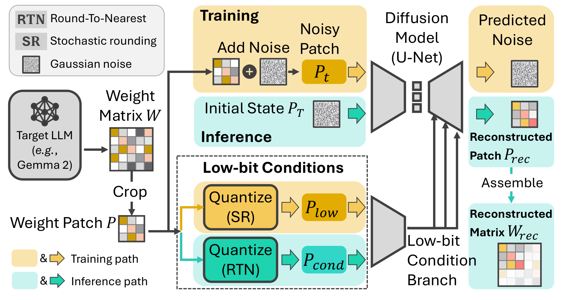
ReRound revisits the final rounding assignments under a fixed quantization setup. For each pretrained LLM, a conditional diffusion model is trained once to produce continuous reconstructed weights (Section 3.2). These reconstructed weights guide rounding decisions affected by midpoint ambiguity and produce candidate quantized integer weight matrices using a position-dependent tolerance metric (Section 3.3). For each matrix, the candidate whose de-quantized weight matrix has leading singular values that best match those of the full-precision matrix is selected (Section 3.4).
3.1 Midpoint-Ambiguous RTN Decisions
Let be a full-precision weight matrix. Consider one quantization group with scale and zero-point ; the same derivation applies independently to every group. For a weight , define its quantized weight as
| (1) |
RTN selects the closer adjacent quantized integer:
| (2) |
The lower and upper assignments incur
| (3) | ||||
Thus, flipping the RTN assignment incurs the additional cost
| (4) |
The cost is smallest at the midpoint and increases toward either adjacent quantized integer. ReRound accordingly gives reconstructed weights greater influence near the midpoint and increasingly preserves RTN away from it.
3.2 Conditional Weight Reconstruction
The flip cost in Eq. (4) identifies where an RTN assignment can be changed at low scalar cost, but not whether the alternative assignment is supported by the joint weight structure. For each pretrained LLM, ReRound trains one conditional diffusion model on local patches from its full-precision weight matrices. The model jointly reconstructs each patch from its low-bit observation, providing a prior learned from the pretrained LLM’s own weights.
Let denote a patch cropped from a full-precision weight matrix . During training, its low-bit condition is formed by group-wise stochastic quantization:
| (5) |
where and are the corresponding scale and zero-point. For an entry , define its quantized weight as , where . Then selects the quantized integer with probability and the quantized integer with probability . Only the condition is quantized; the reconstruction target remains the full-precision patch . ReRound models the conditional distribution using conditional diffusion (41).
At diffusion step , Gaussian noise produces
| (6) |
where determines the noise level. The denoiser receives , , and and predicts the added noise:
| (7) |
During diffusion inference, let be the patches cropped from a weight matrix of the pretrained LLM. Each patch is conditioned on its deterministic RTN quantization:
| (8) |
Starting from , the conditional reverse process produces
| (9) |
where denotes reverse diffusion from step to step . The reconstructed patches are returned to their original locations to form the reconstructed matrix . Because each patch is reconstructed jointly, each reconstructed entry depends on its low-bit observation and the surrounding entries in the patch. The reconstructed matrix is used only to guide rounding and is not deployed as the final weight matrix.
3.3 Reconstruction-Guided Rounding

ReRound uses the reconstructed weights to propose alternative floor-or-ceiling assignments under the fixed PTQ quantization parameters. Let and be corresponding entries of and the reconstructed matrix . Using the fixed scale and zero-point , we map both to the same quantized weight space:
| (10) |
Using , , and from Eq. (19), define
| (11) | ||||||
The reconstructed weight proposes changing RTN only when . Thus, reconstruction-guided rounding can only switch RTN to the opposite adjacent quantized integer. Whether the proposal is accepted depends on the original quantized weight’s position within its quantization interval. Define its distance to the nearest quantized integer as
| (12) |
Here, at the midpoint and decreases toward zero near either adjacent quantized integer. By Eq. (4), for a fixed scale , larger corresponds to a lower RTN flip cost.
The position-dependent tolerance metric for a reconstruction-guided proposal depends on . Given a tolerance parameter , ReRound defines
| (13) |
where . The parameter defines the midpoint region , where . Outside this region, controls how quickly the tolerance metric decreases toward either adjacent quantized integer.
The reconstruction deviation, measured in quantization-step units, is
| (14) |
The candidate assignment for tolerance parameter is
| (15) |
Applying Eq. (15) element-wise produces one candidate quantized integer weight matrix for each tolerance parameter . Different tolerance parameters produce different rounding candidates, while all other quantization settings remain fixed. The next section selects one candidate for each weight matrix.
3.4 Candidate Selection via Spectral Preservation

| Gemma 2 2B | Gemma 3 1B | Qwen3 1.7B | ||||||||||||||
| Method | WinoGrande | PIQA | BoolQ | SIQA | Avg. | WinoGrande | PIQA | BoolQ | SIQA | Avg. | WinoGrande | PIQA | BoolQ | SIQA | Avg. | |
| 16-bit | 69.0 | 79.3 | 72.7 | 51.4 | 68.1 | 58.8 | 74.9 | 66.5 | 42.9 | 60.8 | 60.9 | 72.6 | 77.5 | 45.2 | 64.1 | |
| W4A16 | RTN channel-wise | 66.2 | 75.6 | 70.2 | 45.6 | 64.4 | 57.2 | 72.1 | 44.9 | 39.8 | 53.5 | 56.5 | 68.4 | 72.3 | 40.1 | 59.3 |
| RTN group-wise, | 67.7 | 78.1 | 69.6 | 50.3 | 66.4 | 57.9 | 72.4 | 62.6 | 42.3 | 58.8 | 57.6 | 70.4 | 77.7 | 42.9 | 62.2 | |
| HQQ, | 68.8 | 78.2 | 71.4 | 50.8 | 67.3 | 58.9 | 73.9 | 54.7 | 42.9 | 57.6 | 59.0 | 69.0 | 75.0 | 42.4 | 61.3 | |
| BNB (FP4) | 67.6 | 77.7 | 61.7 | 50.6 | 64.4 | 58.4 | 73.5 | 55.5 | 42.1 | 57.4 | 57.8 | 68.9 | 76.7 | 43.1 | 61.6 | |
| Hadamard + RTN, | 68.0 | 78.0 | 58.3 | 49.6 | 63.5 | 58.4 | 73.4 | 63.1 | 42.4 | 59.3 | 57.1 | 66.5 | 72.4 | 41.3 | 59.3 | |
| ReRound | 68.7 | 78.6 | 72.0 | 50.1 | 67.4 | 59.3 | 73.3 | 61.9 | 42.6 | 59.3 | 58.6 | 70.3 | 78.3 | 43.2 | 62.6 | |
| W3A16 | RTN channel-wise | 51.3 | 55.4 | 61.5 | 34.3 | 50.6 | 50.2 | 52.6 | 47.3 | 33.9 | 46.0 | 50.5 | 53.1 | 40.1 | 34.4 | 44.5 |
| RTN group-wise, | 63.2 | 73.5 | 68.3 | 42.6 | 61.9 | 55.5 | 65.9 | 60.9 | 38.9 | 55.3 | 53.4 | 62.5 | 62.9 | 37.5 | 54.1 | |
| HQQ, | 62.3 | 73.5 | 60.9 | 44.3 | 60.2 | 55.6 | 67.4 | 60.2 | 38.1 | 55.3 | 48.5 | 54.4 | 51.4 | 34.2 | 47.1 | |
| Hadamard + RTN, | 61.6 | 76.1 | 63.8 | 46.0 | 61.9 | 55.0 | 67.4 | 48.2 | 37.7 | 52.1 | 49.6 | 54.7 | 48.2 | 34.3 | 46.7 | |
| ReRound | 63.8 | 73.1 | 68.6 | 42.6 | 62.0 | 56.2 | 65.5 | 61.3 | 38.9 | 55.5 | 52.5 | 62.7 | 64.6 | 36.9 | 54.2 | |
Reconstruction-guided rounding produces one candidate quantized integer weight matrix for each tolerance parameter . ReRound selects the candidate whose de-quantized weight matrix has leading singular values that most closely match those of the full-precision matrix . These values summarize the strengths of the matrix’s dominant transformation modes, providing a matrix-level criterion without requiring activation data.
Figure 4 illustrates the selection process. For each tolerance parameter , the candidate quantized integer weight matrix is de-quantized using the fixed PTQ parameters:
| (16) |
where and denote the fixed scales and zero-points, applied group-wise when needed. The candidate is de-quantized only for spectral comparison.
Let be the smaller dimension of . We compare the leading singular values, where . This choice adapts to the matrix size and uses at most singular values. Let and denote their leading singular values, ordered from largest to smallest.
| (17) |
where ensures numerical stability. ReRound selects
| (18) |
The selected provides the final quantized integer assignments and, together with the fixed scales and zero-points, defines the quantized representation of .
4 Experiments
4.1 Experimental Setup
We summarize the main settings below; further implementation details are provided in the supplementary material.
Models and evaluation.
Our full baseline comparison includes Gemma 2 2B (19), Gemma 3 1B (18), Qwen3 1.7B (44), OLMo 2 1B (30), and SmolLM2 1.7B (1). We further evaluate whether ReRound consistently improves RTN across Llama 3.2 1B (20), Pythia 1.4B (4), and Phi-2 2.7B (22). We evaluate zero-shot accuracy on WinoGrande (34), PIQA (5), BoolQ (10), and SIQA (35) using the LM Evaluation Harness (17). For SINQ (28), we adopt its quantization scales and also report perplexity on WikiText-2 (27) and C4 (31).
| OLMo 2 1B | SmolLM2 1.7B | ||||||||||
| Method | WinoGrande | PIQA | BoolQ | SIQA | Avg. | WinoGrande | PIQA | BoolQ | SIQA | Avg. | |
| 16-bit | 64.6 | 75.2 | 62.3 | 43.4 | 61.4 | 66.1 | 77.3 | 72.5 | 44.3 | 65.1 | |
| W4A16 | RTN channel-wise | 59.4 | 72.4 | 63.2 | 42.2 | 59.3 | 58.1 | 72.2 | 64.3 | 40.1 | 58.7 |
| RTN group-wise, | 63.5 | 74.9 | 51.7 | 42.3 | 58.1 | 63.5 | 76.2 | 68.3 | 42.8 | 62.7 | |
| HQQ, | 64.3 | 74.8 | 59.9 | 42.5 | 60.4 | 61.8 | 75.4 | 67.3 | 43.0 | 61.9 | |
| BNB (FP4) | 61.9 | 74.7 | 64.3 | 43.4 | 61.1 | 62.7 | 76.3 | 54.4 | 44.0 | 59.3 | |
| Hadamard + RTN, | 63.3 | 75.5 | 52.3 | 43.3 | 58.6 | 62.8 | 74.8 | 68.3 | 42.0 | 62.0 | |
| ReRound | 63.9 | 75.4 | 54.4 | 43.7 | 59.4 | 65.1 | 76.7 | 67.3 | 42.3 | 62.9 | |
| W3A16 | RTN channel-wise | 51.1 | 57.6 | 38.8 | 33.8 | 45.4 | 48.2 | 51.0 | 49.4 | 33.3 | 45.5 |
| RTN group-wise, | 58.7 | 71.2 | 47.7 | 39.5 | 54.3 | 57.9 | 70.0 | 58.0 | 38.2 | 56.0 | |
| HQQ, | 56.3 | 67.1 | 58.0 | 36.4 | 54.4 | 53.4 | 60.8 | 58.9 | 37.8 | 52.8 | |
| Hadamard + RTN, | 55.6 | 68.4 | 42.1 | 35.5 | 50.4 | 51.5 | 59.7 | 45.0 | 36.1 | 48.1 | |
| ReRound | 57.7 | 71.4 | 51.4 | 39.9 | 55.1 | 57.5 | 71.0 | 60.6 | 38.3 | 56.9 | |
Quantization settings.
In the main RTN and ReRound experiments, we use asymmetric uniform weight quantization. W4A16 and W3A16 denote 4-bit and 3-bit weight quantization, respectively, both with 16-bit activations. All group-wise methods use group size . For all evaluated quantization methods, we quantize the transformer linear layers and the output logit layer (lm_head). ReRound uses the same scales, zero-points, group size, and layer coverage as group-wise RTN; only selected quantized integer assignments differ. It therefore preserves the same low-bit representation and inference procedure as RTN.
Baselines.
Diffusion training and inference.
For each pretrained LLM, we train one conditional diffusion model (41) on two GPUs using full-precision patches paired with 2-bit conditions generated by stochastic rounding (SR). Diffusion inference uses one GPU to reconstruct from deterministic 2-bit RTN conditions. The same reconstructed matrix is reused for the 3- and 4-bit ReRound runs. For SINQ, we instead train separate models for 3-bit and 4-bit conditions, using SR during training and RTN during diffusion inference.
ReRound PTQ.
For each target bit width, ReRound uses one GPU to map and to the same quantized weight space, construct candidate quantized integer weight matrices over , and select one candidate for each weight matrix by matching the leading singular values of its de-quantized weight matrix to those of . It changes at most of the RTN quantized integer assignments in each matrix and uses the same formulation across models. All diffusion-based reconstruction and ReRound PTQ stages use only the pretrained model’s weights, without activation or text calibration samples.
| Model | Method | WinoGrande | PIQA | BoolQ | SIQA | Avg. |
|---|---|---|---|---|---|---|
| Gemma 2 2B | 16 bits | 69.0 | 79.3 | 72.7 | 51.4 | 68.1 |
| GPTQ, | 66.5 | 78.6 | 70.9 | 50.8 | 66.7 | |
| AdaRound, | 68.2 | 78.5 | 70.6 | 50.2 | 66.9 | |
| SignRound, | 67.9 | 78.4 | 70.8 | 51.1 | 67.0 | |
| CafeQ | 66.9 | 78.0 | 67.1 | 51.4 | 65.9 | |
| ReRound | 68.7 | 78.6 | 72.0 | 50.1 | 67.4 | |
| Gemma 3 1B | 16 bits | 58.8 | 74.9 | 66.5 | 42.9 | 60.8 |
| GPTQ, | 58.0 | 73.9 | 56.8 | 42.3 | 57.8 | |
| AdaRound, | 59.1 | 73.0 | 61.4 | 42.0 | 58.9 | |
| SignRound, | 58.5 | 73.2 | 63.5 | 41.3 | 59.1 | |
| ReRound | 59.3 | 73.3 | 61.9 | 42.6 | 59.3 |
| Bits | Method | Rec. | Pos. | Spec. | Wino. | PIQA | BoolQ | SIQA | Avg. |
|---|---|---|---|---|---|---|---|---|---|
| W4A16 | RTN (group-wise, ) | – | – | – | 63.5 | 74.9 | 51.7 | 42.3 | 58.1 |
| Matched random flips | – | ✓ | ✓ | 63.5 | 75.3 | 51.8 | 43.3 | 58.5 | |
| Midpoint window | ✓ | – | ✓ | 63.8 | 75.6 | 50.7 | 43.6 | 58.4 | |
| Weight-MSE selection | ✓ | ✓ | – | 64.6 | 75.5 | 50.6 | 44.0 | 58.7 | |
| ReRound | ✓ | ✓ | ✓ | 63.9 | 75.4 | 54.4 | 43.7 | 59.4 | |
| W3A16 | RTN (group-wise, ) | – | – | – | 58.7 | 71.2 | 47.7 | 39.5 | 54.3 |
| Matched random flips | – | ✓ | ✓ | 57.4 | 70.2 | 49.3 | 39.3 | 54.1 | |
| Midpoint window | ✓ | – | ✓ | 59.0 | 71.2 | 48.0 | 39.6 | 54.5 | |
| Weight-MSE selection | ✓ | ✓ | – | 58.7 | 71.2 | 47.7 | 39.5 | 54.3 | |
| ReRound | ✓ | ✓ | ✓ | 57.7 | 71.4 | 51.4 | 39.9 | 55.1 |
4.2 Comparison with Calibration-Free PTQ
Tables 1 and 2 compare ReRound with calibration-free weight-only PTQ methods across five LLMs. ReRound improves its matched group-wise RTN baseline for every model at both bit widths, with gains of – points at 3 bits and – points at 4 bits. Because the scales, zero-points, group size, and layer coverage are fixed, these gains come solely from revising selected quantized integer assignments.
At 3 bits, ReRound achieves the highest four-task average on every model, showing the benefit of revisiting midpoint-ambiguous decisions under aggressive quantization. At 4 bits, it achieves or matches the best average on four of the five models. On OLMo 2 1B, HQQ and BNB FP4 obtain averages of and , respectively, compared with for ReRound. Nevertheless, ReRound raises its matched group-wise RTN baseline from to , the largest 4-bit gain in the comparison. Thus, even when another quantization parameterization performs better, revising selected quantized integer assignments substantially improves the fixed RTN quantization setup.
| Method | WinoGrande | PIQA | BoolQ | SIQA | Acc Avg. | Wiki2 | C4 | PPL Avg. | |
|---|---|---|---|---|---|---|---|---|---|
| 16-bit | 60.9 | 72.6 | 77.5 | 45.2 | 64.1 | 16.72 | 19.25 | 17.99 | |
| W4A16 | SINQ-scale RTN, | – | – | – | – | – | 17.14 | 19.83 | 18.49 |
| SINQ-scale RTN, | 59.0 | 71.5 | 75.1 | 42.9 | 62.1 | 17.19 | 19.87 | 18.53 | |
| SINQ-scale ReRound, | 59.7 | 71.7 | 74.8 | 44.0 | 62.6 | 17.09 | 19.83 | 18.46 | |
| W3A16 | SINQ-scale RTN, | – | – | – | – | – | 22.39 | 24.88 | 23.64 |
| SINQ-scale RTN, | 54.1 | 67.4 | 66.1 | 40.6 | 57.1 | 23.27 | 25.25 | 24.26 | |
| SINQ-scale ReRound, | 55.6 | 66.8 | 65.9 | 40.9 | 57.3 | 23.14 | 24.97 | 24.06 |
4.3 Comparison with Calibration-Based PTQ
Table 3 compares ReRound with calibration-based PTQ methods under W4A16 quantization, together with CafeQ on Gemma 2 2B. ReRound achieves the highest four-task average among the quantized methods on both models. The strongest calibration-based method, SignRound, reaches averages of on Gemma 2 2B and on Gemma 3 1B, whereas ReRound achieves and , respectively. Thus, ReRound surpasses the best calibration-based result by and points without using activation or text calibration data. These results show that revisiting midpoint-ambiguous rounding decisions with a weight prior learned from the pretrained model’s own weights can compete effectively with calibration-data-driven PTQ.
4.4 Ablation of ReRound Components
Table 4 isolates reconstruction guidance, the position-dependent tolerance metric, and spectral selection on OLMo 2 1B. Each ablation replaces one component while retaining the other two. Matched random flips remove reconstruction guidance by randomly choosing the same number of quantized integer assignment changes as ReRound. Midpoint window replaces the position-dependent tolerance metric with , while weight-MSE selection uses element-wise weight MSE instead of spectral discrepancy. Full ReRound achieves the highest four-task average at both bit widths, improving group-wise RTN by points at W4 and points at W3. Replacing any component lowers the average accuracy.
4.5 Alternative Quantization Parameters
Table 5 evaluates ReRound using quantization parameters generated by another PTQ method. We use SINQ parameters and compare RTN with ReRound under the same reproduced setting, including SINQ’s reported RTN perplexities for reference. At 4 bits, ReRound increases the four-task average from to and reduces average perplexity from to . At 3 bits, it increases the average from to and reduces average perplexity from to . Thus, ReRound also improves quantization setups from other PTQ methods.
4.6 RTN Improvements on Additional Models
Figure 5 extends the five-model comparison with Llama 3.2 1B, Pythia 1.4B, and Phi-2 2.7B. ReRound improves group-wise RTN for every model at both 3 and 4 bits. The gains range from to points at 4 bits and from to points at 3 bits. Because ReRound and RTN use the same scales, zero-points, group size, and layer coverage, these differences arise solely from revising selected quantized integer assignments. The positive gains on the three additional models extend the same trend beyond those used in the full calibration-free comparison. Complete per-task results for these models are provided in the supplementary material.
| Model | Diffusion Training (h) | Diffusion Inference (h) | ReRound PTQ (s) |
|---|---|---|---|
| Gemma 2 2B | 2.52 | 9.55 | 105 |
| Gemma 3 1B | 2.69 | 3.65 | 42 |
| Qwen3 1.7B | 1.76 | 6.29 | 74 |
| OLMo 2 1B | 1.77 | 9.32 | 57 |
| SmolLM2 1.7B | 3.43 | 6.25 | 124 |
4.7 Offline Runtime
Table 6 reports the offline cost of ReRound. Diffusion training is performed once per model on two GPUs, and one-GPU diffusion inference produces the reconstructed matrix for reuse across bit widths. With this shared reconstruction, ReRound PTQ averages to seconds across W3 and W4. All additional computation occurs before deployment; the resulting quantized model uses the same low-bit representation and inference procedure as RTN.
5 Discussion and Limitations
ReRound revises RTN assignments while keeping scales and zero-points fixed, so it can refine quantization parameters produced by other PTQ methods. However, its candidate set remains constrained by these parameters, motivating joint optimization of quantization parameters and reconstruction-guided rounding. Although the approach may extend beyond LLMs, we evaluate only small LLMs.
ReRound also requires a separate diffusion model for each pretrained LLM, introducing model-specific offline cost. Reusing reconstructed weights across bit widths reduces this cost, but scaling to many models remains expensive. In addition, spectral selection operates only in weight space and may not identify the best candidate for every downstream task, while patch-based reconstruction may miss long-range and cross-layer dependencies. Reducing reconstruction cost, transferring weight priors across models, and using broader structural criteria are promising directions.
6 Conclusion
We presented ReRound, a calibration-free framework that revisits midpoint-ambiguous RTN decisions after quantization parameters are fixed. ReRound learns a diffusion prior from the model’s own weights, uses it to guide floor-or-ceiling changes, and selects candidate matrices through spectral preservation. Across diverse LLMs, it consistently improves 3- and 4-bit weight-only PTQ without activation or text calibration data. Because ReRound changes only selected quantized integer assignments, the quantization parameters, low-bit representation, and inference procedure remain unchanged. These results show that structural patterns in pretrained weights can serve as an effective prior for resolving ambiguous rounding decisions.
Appendix A Quantization Notation
Let be a full-precision weight in a quantization group with scale and zero-point . Applying these fixed quantization parameters gives
| (19) |
We refer to the continuous floating-point value before rounding as the quantized floating-point weight, or simply the quantized weight. Rounding produces a discrete quantized integer . Mapping back to the original weight space gives the corresponding dequantized weight, .
Appendix B Software Environment
We use the same software environment for diffusion-based weight recovery, post-training quantization (PTQ), and language-model evaluation. PyTorch is compiled with CUDA 12.4. Table 7 lists the main packages used in our experiments. For weight recovery, we follow the DeepFloyd IF Stage-II (11; 32) implementation used by Vavilala et al. (41) and initialize the model from the IF-II-M-v1.0 pretrained checkpoint.
| Package | Version |
|---|---|
| PyTorch | 2.5.1+cu124 |
| TorchVision | 0.20.1+cu124 |
| CUDA runtime | 12.4.127 |
| cuDNN | 9.1.0.70 |
| Accelerate | 1.1.1 |
| Transformers | 4.57.1 |
| Diffusers | 0.35.2 |
| Datasets | 5.0.0 |
| lm-eval | 0.4.11 |
| Hugging Face Hub | 0.36.0 |
| Tokenizers | 0.22.1 |
Appendix C Diffusion Training and Inference Details
Diffusion architecture and conditioning.
Following Vavilala et al. (41), we build the weight recovery model from DeepFloyd IF Stage II (IF-II-M-v1.0). We add a ControlNet to the pretrained U-Net and use the low-bit weight patch as the ControlNet condition. During training, the U-Net remains frozen and only the ControlNet is updated. The ControlNet text-encoder pooling and projection layers are also kept frozen.
Because weight recovery does not require natural-language information, we use a precomputed T5 embedding of an empty prompt for all training and inference runs. Each weight patch and its low-bit condition contain one channel. We repeat each of them across three channels to match the input format of the pretrained diffusion model.
Weight-patch construction.
For each target LLM, we extract its two-dimensional weight matrices, including the language-model head. We exclude token embeddings and normalization parameters. The extracted weights are converted to FP32 and divided into patches.
Before they are given to the diffusion model, the weights in each quantization group are normalized to the range using the minimum and range of that group. We use asymmetric group-wise quantization with a group size of 128 to generate the low-bit conditions.
During training, we first randomly select a weight matrix and then randomly crop a patch from that matrix. This allows the model to observe patches from different layers and different locations throughout training. If a matrix is smaller than the patch size, the patch is padded to , and a validity mask identifies the original, non-padded entries. We also horizontally flip each training patch with probability .
Each normalized full-precision target patch is paired with a 2-bit condition generated by stochastic rounding (SR). SR rounds each quantized weight to its lower or upper neighboring integer according to its fractional part. The resulting 2-bit patch is used only as the condition, while the training target remains the normalized full-precision patch.
Optimization and hardware.
We train a separate diffusion model for each target LLM using two NVIDIA GeForce RTX 4090 GPUs. Each model is trained for five epochs, with randomly sampled patches per epoch. The batch size is 32 per GPU, giving an effective batch size of 64 across the two GPUs, without gradient accumulation.
We optimize the ControlNet using AdamW with a constant learning rate of and no learning-rate scheduler. We use the default PyTorch AdamW settings: , , , and weight decay . The script-level random seed is set to 1.
Diffusion inference and matrix assembly.
Diffusion inference is performed on one NVIDIA GeForce RTX 4090 GPU with a batch size of 128. Unlike training, inference uses deterministic 2-bit RTN conditions. We use DDPM sampling with the super27 timestep-respacing schedule, which contains 27 reverse-diffusion steps.
During inference, we process all patches of each weight matrix in a fixed order. We begin at the top-left corner, move from left to right, and then continue to the next rows. If the matrix size is not divisible by 64, we add a final patch aligned with the bottom or right edge so that every weight is covered.
The diffusion model predicts each patch in the normalized space. We then map the predicted values back to the original full-precision weight space using the minimum and range of their corresponding quantization groups. Each recovered patch is written back to its original location. After all patches are processed, they are combined to form the complete recovered weight matrix .
For ReRound, we train one diffusion model per target LLM using 2-bit SR conditions. During diffusion inference, the model reconstructs from deterministic 2-bit RTN conditions. The resulting is computed once and reused unchanged for both the 3-bit and 4-bit ReRound experiments.
For the SINQ experiments, we instead train separate diffusion models for the 3-bit and 4-bit conditions. At each precision, SR is used to generate the training conditions, whereas deterministic RTN is used to generate the conditions during diffusion inference.
Appendix D ReRound Settings
ReRound PTQ.
For each target bit width, ReRound uses one GPU to map and to the same quantized weight space, construct candidate quantized integer weight matrices over , and select one candidate for each weight matrix by matching the leading singular values of its dequantized weight matrix to those of . We use separate candidate sets for the transformer linear layers and the output logit layer (lm_head). Table 8 reports these candidate sets and the position-dependent tolerance parameter . The same settings are used for the 3-bit and 4-bit experiments. A candidate with corresponds to retaining the RTN assignments. ReRound changes at most of the RTN quantized integer assignments in each matrix and uses the same formulation across models. All diffusion-based reconstruction and ReRound PTQ stages use only the pretrained model’s weights, without activation or text calibration samples. In Eq. (13) of the main paper, we set for all models and bit widths, corresponding to the central midpoint ambiguity region .
| Model | |||
|---|---|---|---|
| Gemma 2 2B | 8 | ||
| Gemma 3 1B | 64 | ||
| Qwen3 1.7B | 128 | ||
| OLMo 2 1B | 32 | ||
| SmolLM2 1.7B | 128 | ||
| Llama 3.2 1B | 64 | ||
| Pythia 1.4B | 8 | ||
| Phi-2 2.7B | 64 | ||
| Falcon 3-1B-Base | 8 |
ReRound with SINQ parameters.
For the experiments using SINQ quantization parameters on Qwen3 1.7B, we follow SINQ’s layer coverage and leave the output logit layer (lm_head) unquantized. Table 9 reports the tolerance candidate sets used for the remaining transformer linear layers. We use at both bit widths. As before, corresponds to retaining the RTN assignments.
| Weight precision | ||
|---|---|---|
| W4 | 8 | |
| W3 | 8 |
Appendix E Additional PTQ Results
E.1 RTN Improvements on Additional Models
Table 10 reports the complete per-task results for Llama 3.2 1B (20), Pythia 1.4B (4), and Phi-2 2.7B (22), together with results on Falcon 3-1B-Base (15). We compare ReRound with group-wise RTN under W4A16 and W3A16 quantization using the same scales, zero-points, group size , and layer coverage. ReRound achieves a higher four-task average for every model at both bit widths, with improvements of up to points. Because the quantization setup remains unchanged, these gains result solely from revising selected quantized integer assignments.
| Model | Bits | Method | WinoGrande | PIQA | BoolQ | SIQA | Avg. |
|---|---|---|---|---|---|---|---|
| Llama 3.2 1B | 16 bits | – | 60.3 | 74.6 | 63.7 | 43.0 | 60.4 |
| W4A16 | RTN group-wise, | 61.1 | 72.4 | 47.1 | 41.8 | 55.6 | |
| ReRound, | 61.3 | 72.5 | 50.4 | 41.7 | 56.5 | ||
| W3A16 | RTN group-wise, | 53.6 | 63.0 | 50.1 | 37.7 | 51.1 | |
| ReRound, | 51.4 | 62.8 | 54.3 | 38.3 | 51.7 | ||
| Falcon 3-1B-Base | 16 bits | – | 61.7 | 74.5 | 71.8 | 45.2 | 63.3 |
| W4A16 | RTN group-wise, | 59.6 | 73.8 | 70.6 | 44.4 | 62.1 | |
| ReRound, | 59.6 | 74.2 | 70.8 | 45.0 | 62.4 | ||
| W3A16 | RTN group-wise, | 58.6 | 71.9 | 62.9 | 41.3 | 58.7 | |
| ReRound, | 59.0 | 72.4 | 63.1 | 40.6 | 58.8 | ||
| Phi-2 2.7B | 16 bits | – | 76.2 | 78.6 | 83.1 | 55.5 | 73.4 |
| W4A16 | RTN group-wise, | 75.5 | 78.6 | 81.1 | 54.7 | 72.5 | |
| ReRound, | 76.5 | 78.2 | 80.7 | 55.6 | 72.8 | ||
| W3A16 | RTN group-wise, | 71.7 | 77.6 | 64.7 | 51.3 | 66.3 | |
| ReRound, | 73.6 | 78.4 | 67.1 | 52.3 | 67.9 | ||
| Pythia 1.4B | 16 bits | – | 57.5 | 71.1 | 63.2 | 41.2 | 58.3 |
| W4A16 | RTN group-wise, | 55.9 | 70.2 | 61.6 | 40.2 | 57.0 | |
| ReRound, | 56.1 | 70.0 | 62.3 | 41.1 | 57.4 | ||
| W3A16 | RTN group-wise, | 52.7 | 67.0 | 52.8 | 38.8 | 52.8 | |
| ReRound, | 53.0 | 66.7 | 55.9 | 39.0 | 53.7 |
E.2 Comparison with AdaRound
Table 11 compares AdaRound and ReRound under W4A16 quantization on OLMo 2 1B (30), SmolLM2 1.7B (1), Llama 3.2 1B (20), Falcon 3-1B-Base (15), Phi-2 2.7B (22), and Qwen3 1.7B (44). Both methods make layer-wise rounding decisions. AdaRound uses 128 calibration samples from C4 (31), while ReRound uses only the pretrained model weights. ReRound achieves a higher four-task average than AdaRound on all six models, with improvements of up to points. Although AdaRound performs better on some individual tasks, ReRound consistently provides higher average accuracy without activation or text calibration data.
| Model | Method | WinoGrande | PIQA | BoolQ | SIQA | Avg. |
|---|---|---|---|---|---|---|
| OLMo 2 1B | AdaRound, | 63.4 | 74.9 | 48.1 | 43.7 | 57.5 |
| ReRound, | 63.9 | 75.4 | 54.4 | 43.7 | 59.4 | |
| SmolLM2 1.7B | AdaRound, | 62.4 | 76.0 | 69.4 | 42.7 | 62.6 |
| ReRound, | 65.1 | 76.7 | 67.3 | 42.3 | 62.9 | |
| Llama 3.2 1B | AdaRound, | 61.2 | 72.7 | 46.2 | 41.9 | 55.5 |
| ReRound, | 61.3 | 72.5 | 50.4 | 41.7 | 56.5 | |
| Falcon 3-1B-Base | AdaRound, | 60.1 | 74.0 | 70.2 | 44.4 | 62.2 |
| ReRound, | 59.6 | 74.2 | 70.8 | 45.0 | 62.4 | |
| Phi-2 2.7B | AdaRound, | 75.9 | 77.9 | 80.7 | 54.7 | 72.3 |
| ReRound, | 76.5 | 78.2 | 80.7 | 55.6 | 72.8 | |
| Qwen3 1.7B | AdaRound, | 58.1 | 70.4 | 77.2 | 42.0 | 61.9 |
| ReRound, | 58.6 | 70.3 | 78.3 | 43.2 | 62.6 |
Appendix F Baseline Implementation Details
Unless otherwise stated, all reimplemented baselines use the model checkpoints and evaluation protocol described in Section G. The transformer linear layers and output logit layer are quantized in the main comparisons, and all group-wise methods use group size .
RTN.
We implement uniform asymmetric RTN using the minimum and maximum weight values for computing the scale and zero-point. Channel-wise RTN computes one pair of quantization parameters per output channel, whereas group-wise RTN computes one pair for every group of 128 consecutive weights along the input dimension.
HQQ.
HQQ version 0.2.8.post1 is applied with the PyTorch backend, quantization axis 1, and group size .
BNB FP4.
BitsAndBytes version 0.49.2 is applied with FP4 weight quantization and BF16 computation. BNB FP4 is evaluated only under W4A16.
Hadamard-transformed RTN.
We apply a normalized Hadamard transform independently to groups of 128 consecutive weights along the input-feature dimension, perform asymmetric RTN in the transformed domain, and then apply the inverse transform.
GPTQ.
GPTQ is applied to all transformer linear layers using asymmetric group-wise quantization with group size . We use 128 calibration sequences of length 2048 from the C4 training split (31) and enable activation ordering and true-sequential quantization. The output logit layer uses asymmetric group-wise RTN with .
AdaRound.
AdaRound uses asymmetric group-wise quantization with group size and 128 calibration sequences of length 2048 from the C4 training split (31). Rounding variables are optimized for 200 iterations using up to 1024 calibration tokens per weight matrix, a learning rate of , and a regularization weight of . To accommodate the large output logit layer, we divide it into blocks covering 1024 vocabulary outputs and optimize each block for 50 iterations.
SignRound.
We use AutoRound version 0.13.1 with its default optimization settings, symmetric group-wise weight quantization, and group size . The output logit layer is also quantized using AutoRound’s built-in quant_lm_head procedure.
Appendix G Models and Evaluation Protocol
Model checkpoints.
Table 12 lists the exact Hugging Face checkpoints used in our experiments.
| Model | Hugging Face checkpoint |
|---|---|
| Gemma 2 2B | google/gemma-2-2b |
| Gemma 3 1B | google/gemma-3-1b-pt |
| Qwen3 1.7B | Qwen/Qwen3-1.7B |
| OLMo 2 1B | allenai/OLMo-2-0425-1B |
| SmolLM2 1.7B | HuggingFaceTB/SmolLM2-1.7B |
| Llama 3.2 1B | meta-llama/Llama-3.2-1B |
| Pythia 1.4B | EleutherAI/pythia-1.4b |
| Phi-2 2.7B | microsoft/phi-2 |
| Falcon 3-1B-Base | tiiuae/Falcon3-1B-Base |
Accuracy evaluation.
All accuracy evaluations are zero-shot and use the standard task configurations in LM Evaluation Harness v0.4.11. We report accuracy (acc) for WinoGrande, BoolQ, and SIQA, and normalized accuracy (acc_norm) for PIQA. Activations remain in 16-bit precision for all weight-quantized experiments. Across all methods, we use random seed 0 and set the NumPy and PyTorch seeds to 1234.

Appendix H Visualization of the Position-Dependent Tolerance Metric
Figure 6 visualizes the position-dependent tolerance metric for different values of . For illustration, we show the tolerance parameters . With , the midpoint ambiguity region is , or equivalently . Within this region, . Outside the midpoint ambiguity region, controls how quickly the tolerance metric decreases toward either adjacent quantized integer. A smaller produces a more gradual decrease, whereas a larger produces a sharper decrease at the boundaries of the midpoint region.

(a) W4

(b) W3
Appendix I Matrix-Wise Revision of RTN Assignments
For each weight matrix, we report the percentage of RTN assignments revised by ReRound. Figures 7 and 8 visualize these revision rates across layers and matrix types under W3 and W4 quantization.
The revision rates vary across matrices and bit widths. Although W3 and W4 reuse the same reconstructed weights, the same matrix can receive different revision rates at the two bit widths. This is because ReRound evaluates the rounding candidates under each target quantization grid and performs spectral selection separately for every matrix. Therefore, the amount of revision depends on both the weight matrix and the target bit width, rather than on the reconstructed weights alone.

(a) W4

(b) W3
Appendix J Continuous Reconstruction for Low-Bit Rounding
ReRound uses a DDPM-based conditional diffusion model (21; 33) to produce continuous reconstructed weights from low-bit weight observations. The reconstructed weights are not deployed as model parameters. They provide an additional signal for reconsidering midpoint-ambiguous RTN assignments.
J.1 Low-Bit Conditioning
Let denote a normalized patch cropped from a full-precision weight matrix . During diffusion training, its low-bit condition is obtained by applying group-wise stochastic rounding (SR):
| (20) |
where denotes the group-wise SR operation. The parameters and are the scale and zero-point used to construct the 2-bit diffusion condition. The subscript distinguishes these conditioning parameters from the target quantization parameters and used later for W3 or W4 rounding.
During diffusion inference, the condition is instead generated deterministically using RTN. For a patch ,
| (21) |
For fixed and , deterministic low-bit quantization is many-to-one. Distinct continuous patches may produce the same RTN condition:
| (22) |
The low-bit condition therefore does not uniquely identify the original full-precision patch.
The diffusion model represents a conditional distribution over full-precision patches given their low-bit conditions (33):
| (23) |
Because the entries of a patch are reconstructed jointly, each reconstructed entry can depend on both its own low-bit observation and the surrounding entries in the patch.
J.2 Conditional Denoising Relation
The following relations are defined under the joint training distribution of the full-precision patch , its stochastic condition , the diffusion timestep , and Gaussian noise . Define
| (24) |
Following the DDPM forward process (21), Gaussian noise is added as
| (25) |
where is sampled independently of . For a fixed and timestep , the forward transition is
| (26) |
Let denote the conditional marginal distribution of the noisy patch. Differentiating this marginal with respect to gives
| (27) |
The second equality follows from
| (28) |
We can also express the conditional score through the added noise. Taking the conditional expectation of Eq. (25) given gives
| (30) |
Solving for the conditional noise mean yields
| (31) |
Combining Eqs. (27) and (31) gives
| (32) |
The conditional diffusion model minimizes
| (33) |
For a fixed input , let
| (34) |
For any noise predictor , the conditional squared error decomposes as
| (35) |
The first term does not depend on , and the second term is minimized when
| (36) |
Therefore, the ideal noise predictor satisfies
| (37) |
Substituting Eq. (37) into Eq. (31) gives
| (38) |
Thus, for the ideal noise predictor, the clean estimate associated with one denoising step equals the conditional mean of the full-precision patch under Gaussian corruption (14; 21). In practice, the learned denoiser approximates this predictor. In addition, the relation above is defined using the stochastic training condition , whereas reverse diffusion is conditioned on the deterministic RTN patch during inference. The final multi-step output is therefore used as a continuous reconstruction, not as an exact recovery of the original patch or as an exact conditional mean.
J.3 Midpoint Distance of Accepted Revisions
Consider a target W3 or W4 quantization group with fixed scale and zero-point . For corresponding entries and of the full-precision and reconstructed matrices, define
| (39) |
where
| (40) |
The RTN assignment, its opposite adjacent assignment, and the reconstruction-based assignment are
| (41) | ||||||
ReRound considers changing RTN only when
| (42) |
The acceptance threshold depends on the fractional position . Define
| (43) |
which equals at the midpoint and decreases toward either adjacent quantized integer.
For tolerance parameter , ReRound uses
| (44) |
where . The parameter defines the central midpoint ambiguity region , in which . Outside this region, the tolerance decreases continuously according to ; it is not set to zero.
The reconstruction deviation in quantization-step units is
| (45) |
A revision is accepted only when
| (46) |
The distance from the original quantized weight to the midpoint boundary is
| (47) |
For the reconstructed assignment to equal the opposite adjacent integer, must reach the other side of the midpoint boundary. Its displacement must therefore be at least . Every accepted revision consequently satisfies
| (48) |
This relation follows directly from the realized reconstruction and the ReRound acceptance conditions. It does not depend on the denoiser being ideal. An RTN assignment can be revised only when the quantized weight’s distance from the midpoint is no larger than the effective tolerance at that position.
J.4 Scalar Error of an Accepted Revision
The squared errors of assigning to the lower and upper adjacent integers are
| (49) |
Switching from RTN to the opposite adjacent assignment adds
| (50) | ||||
Using Eq. (48), an accepted revision satisfies
| (51) |
The tolerance rule therefore bounds the additional scalar squared quantization error of each accepted revision relative to RTN. This is a scalar weight-space relation and does not characterize changes in model outputs or downstream task accuracy.
J.5 Spectral Comparison with RTN
For each tolerance parameter , applying the ReRound rule element-wise produces a quantized integer matrix . Its dequantized matrix is
| (52) |
where and are the fixed target quantization parameters. The candidate retains all RTN assignments:
| (53) |
For each candidate, ReRound measures
| (54) |
where denotes the leading singular values, and provides numerical stability. For a matrix evaluated by the candidate search, ReRound selects
| (55) |
Because is included in , RTN is one of the candidates in this comparison. It follows directly from the selection rule that
| (56) |
The selected candidate therefore has no larger discrepancy than RTN under the spectral criterion used for selection. This inequality applies only to the spectral discrepancy used for candidate selection.
The conditional model produces the continuous reconstruction used to propose alternative assignments. The position-dependent tolerance determines which proposals are accepted, while spectral selection compares the resulting matrices with the unchanged RTN candidate.
Appendix K Weight Reconstruction and ReRound Procedures
Algorithms 1 and 2 present the complete procedures for conditional weight reconstruction and ReRound PTQ. All quantization operations are applied group-wise, and all matrix operations in Algorithm 2 are element-wise unless otherwise stated. The reconstructed matrices are produced once and reused for the W3 and W4 ReRound runs.
References
- SmolLM2: when smol goes big—data-centric training of a fully open small language model. In COLM, Cited by: §E.2, §4.1.
- QuaRot: outlier-free 4-bit inference in rotated llms. In NeurIPS, pp. 100213–100240. Cited by: §1, §2.1, §4.1.
- Half-quadratic quantization of large machine learning models. External Links: Link Cited by: §2.1.
- Pythia: a suite for analyzing large language models across training and scaling. In ICML, pp. 2397–2430. Cited by: §E.1, §4.1.
- PIQA: reasoning about physical commonsense in natural language. In AAAI, pp. 7432–7439. Cited by: §4.1.
- Diffusion model based signal recovery under 1-bit quantization. In AAAI, pp. 20400–20408. Cited by: §2.3.
- SignRoundV2: closing the performance gap in extremely low-bit post-training quantization for llms. arXiv preprint arXiv:2512.04746. Cited by: §2.2.
- Optimize weight rounding via signed gradient descent for the quantization of llms. In Findings of EMNLP, pp. 11332–11350. Cited by: §2.2.
- Diffusion posterior sampling for general noisy inverse problems. In ICLR, Cited by: §2.3.
- BoolQ: exploring the surprising difficulty of natural yes/no questions. In NAACL-HLT, pp. 2924–2936. Cited by: §4.1.
- DeepFloyd IF: a text-to-image diffusion model. Note: https://stability.ai/news-updates/deepfloyd-if-text-to-image-modelStability AI Cited by: Appendix B.
- QLoRA: efficient finetuning of quantized llms. In NeurIPS, pp. 10088–10115. Cited by: §4.1.
- Interpreting the weight space of customized diffusion models. In NeurIPS, pp. 137334–137371. Cited by: §2.3.
- Tweedie’s formula and selection bias. Journal of the American Statistical Association, pp. 1602–1614. Cited by: §J.2, §J.2.
- The falcon 3 family of open models. External Links: Link Cited by: §E.1, §E.2.
- GPTQ: accurate post-training quantization for generative pre-trained transformers. arXiv preprint arXiv:2210.17323. Cited by: §1, §2.1.
- The language model evaluation harness. Note: ZenodoVersion v0.4.11, released February 2026 Cited by: §4.1.
- Gemma 3 technical report. arXiv preprint arXiv:2503.19786. Cited by: §4.1.
- Gemma 2: improving open language models at a practical size. arXiv preprint arXiv:2408.00118. Cited by: §4.1.
- The llama 3 herd of models. arXiv preprint arXiv:2407.21783. Cited by: §E.1, §E.2, §4.1.
- Denoising diffusion probabilistic models. In NeurIPS, pp. 6840–6851. Cited by: §J.2, §J.2, Appendix J.
- Phi-2: the surprising power of small language models. External Links: Link Cited by: §E.1, §E.2, §4.1.
- FlexRound: learnable rounding based on element-wise division for post-training quantization. In ICML, pp. 18913–18939. Cited by: §2.2.
- AWQ: activation-aware weight quantization for on-device llm compression and acceleration. GetMobile: Mobile Computing and Communications, pp. 12–17. Cited by: §1, §2.1.
- SpinQuant: llm quantization with learned rotations. In ICLR, Cited by: §2.1.
- Quantized compressed sensing with score-based generative models. arXiv preprint arXiv:2211.13006. Cited by: §2.3.
- Pointer sentinel mixture models. In ICLR, Cited by: §4.1.
- SINQ: sinkhorn-normalized quantization for calibration-free low-precision llm weights. In ICML, Cited by: §2.1, §4.1, §4.1.
- Up or down? adaptive rounding for post-training quantization. In ICML, pp. 7197–7206. Cited by: §2.2.
- OLMo 2 furious. arXiv preprint arXiv:2501.00656. Cited by: §E.2, §4.1.
- Exploring the limits of transfer learning with a unified text-to-text transformer. Journal of machine learning research 21, pp. 140:1–140:67. Cited by: §E.2, Appendix F, Appendix F, §4.1.
- Photorealistic text-to-image diffusion models with deep language understanding. In NeurIPS, pp. 36479–36494. Cited by: Appendix B.
- Image super-resolution via iterative refinement. IEEE Transactions on Pattern Analysis and Machine Intelligence, pp. 4713–4726. Cited by: §J.1, Appendix J.
- WinoGrande: an adversarial winograd schema challenge at scale. In AAAI, pp. 8732–8740. Cited by: §4.1.
- Social iqa: commonsense reasoning about social interactions. In EMNLP-IJCNLP, pp. 4462–4472. Cited by: §4.1.
- OmniQuant: omnidirectionally calibrated quantization for large language models. In ICLR, Cited by: §2.1.
- Diffusion-based neural network weights generation. In ICLR, Cited by: §2.3.
- FlatQuant: flatness matters for llm quantization. In ICML, Cited by: §2.1.
- CafeQ: calibration-free quantization via learned transformations and adaptive rounding. arXiv preprint arXiv:2511.19705. Cited by: §2.2.
- Learning single index models with diffusion priors. arXiv preprint arXiv:2505.21135. Cited by: §2.3.
- Dequantization and color transfer with diffusion models. In WACV, pp. 9630–9639. Cited by: Appendix B, Appendix C, §2.3, §3.2, §4.1.
- Neural network diffusion. arXiv preprint arXiv:2402.13144. Cited by: §2.3.
- SmoothQuant: accurate and efficient post-training quantization for large language models. In ICML, pp. 38087–38099. Cited by: §1, §2.1.
- Qwen3 technical report. arXiv preprint arXiv:2505.09388. Cited by: §E.2, §4.1.