Adiabatic Perturbations in GW170817-Compatible Einstein-Gauss-Bonnet Inflation
Abstract
We study the adiabaticity of the cosmological perturbations in the context of inflationary Einstein-Gauss-Bonnet theories. We focus on viable inflationary Einstein-Gauss-Bonnet theories which are compatible with the current Cosmic Microwave Background radiation experiments and also are compatible with the GW170817 observations. We derive the effects of the adiabaticity requirement on the Einstein-Gauss-Bonnet physical parameters and we show that the sound speed of the scalar perturbations and the propagation speed of the tensor perturbations are constrained. We consider two classes of inflationary viable and GW170817-compatible theories, and in the first class the adiabaticity is not violated during inflation, while in the second class the adiabaticity is violated only at the end of inflation. We discuss the effects of the adiabaticity violation in the second class of models. From our analysis, it seems that only one class of viable EGB inflationary theories, which is also compatible with the GW170817 event, is free from adiabaticity pathologies.
I Introduction
The next decade is expected to be quite fascinating, since major experiments having to do with cosmology are expected to commence. The most important aim of these experiments is to reveal whether the inflationary regime of our Universe took place primordially. Undoubtedly, the primordial era of our Universe has long been theorized and the only theory that can actually be tested is inflation [1, 2, 3, 4, 5, 6]. The inflation theory is a theoretical construction that solves the flatness and horizon problems of the standard Big Bang cosmology and currently is constrained by the Cosmic Microwave Background (CMB) experiments. A smoking gun signature of inflation would be the observation of the B-modes in the CMB polarization. This is the aim of the near future CMB experiments like the Simons Observatory [7] and the LiteBird experiment [8]. Apart from the CMB, the inflationary era can be indirectly revealed by the existence of a stochastic gravitational wave background with cosmological origin, and this will be probed in the mid 2030 by the future gravitational wave experiments [9, 10, 11, 12, 13, 14, 15, 16, 17]. NANOGrav already confirmed the existence of a stochastic gravitational wave background in 2023 [18], but it is highly unlikely that such a background can be attributed solely to inflation [19, 20].
Apart from the single scalar field modelling of inflation [1, 2, 3, 4, 5, 6], there is also the modified gravity description [21, 22, 23, 6], and two mainstream modified gravity theories are of fundamental importance for modelling inflation, gravity [24, 25, 27, 26, 28, 29, 30, 31, 32, 33, 34, 35, 36, 37, 38, 39, 40, 41, 42, 43, 44, 45, 46] and Einstein-Gauss-Bonnet (EGB) gravity [47, 48, 49, 50, 51, 52, 53, 54, 55, 56, 57, 58, 59, 60, 61, 62, 63, 64, 65, 66, 67, 68, 69, 70, 71, 72, 73, 74, 75, 76, 77, 78]. Both these theories are very well theoretically motivated, because the EGB term and the gravity emerge as the one-loop corrections of a single scalar field in its vacuum configuration, which is conformally or minimally coupled. Indeed, the quantum corrections of the scalar field action has the form [71],
| (1) | ||||
with the parameters , being dimensionful constants. Doubts were cast on EGB theories and Horndeski theories in general back in 2017, with the release of the GW170817 observation [79, 80, 81, 82], see Refs. [83, 84, 85, 86, 87]. The GW170817 constraint on the gravitational wave speed is,
| (2) |
and since EGB and many Horndeski theories in general predict a speed of tensor perturbations distinct from unity in natural units, these theories were cast out from being viable inflationary theories. A remedy however for EGB theories was proposed in Refs. [72, 73, 74, 75], which solved the viability issues of EGB theories.
In this work we focus on the viable EGB inflationary theories of Refs. [72, 73, 74, 75] and we study an aspect of these theories that has never been formally addressed in the literature, namely the adiabaticity of the cosmological perturbations of these theories. Specifically, we shall study two distinct classes of viable EGB theories, the constrained EGB inflationary theories developed in [72, 73, 74] and the unconstrained EGB inflationary theories [75]. We shall analyze the adiabaticity criteria for general inflationary EGB theories, and we shall study which of the two classes respects the adiabaticity criteria. As we demonstrate, the constrained EGB theories violate the adiabaticity criteria at the end of the inflationary era, in the last few -foldings, thus particle creation takes place at the end of inflation, but also the power spectrum is affected by the non-adiabaticity of the perturbations. However, the unconstrained EGB theories do not violate the adiabaticity criteria.
For the rest of this work, we assume that the spacetime is described by a flat Friedmann-Robertson-Walker (FRW) spacetime, with line element,
| (3) |
where is the scale factor and also the Hubble rate is .
II Adiabatic Perturbations and the Adiabatic Vacuum of EGB Theories
II.1 Adiabatic Cosmological Perturbation Definition
In this section we thoroughly discuss the meaning of the adiabatic vacuum and the adiabatic perturbations in cosmology. The terminology ”adiabatic” in curved spacetime quantum field theories refers essentially to the quantum mechanical adiabaticity and not the thermodynamical adiabatic processes. The term adiabatic means essentially that the transitions between instantaneous eigenmodes is suppressed, and no Bogoliubov mixing occurs. If no Bogoliubov mixing occurs in the perturbation modes of a cosmological theory, no particle production occurs and vice versa. This occurs in cosmological theories where the background parameters vary very slowly compared to the oscillation time scale of the field modes.
In cosmological theories, the perturbations satisfy an evolution equation of the form,
| (4) |
where is and are the Fourier modes of the perturbations, is the scale factor and is the conformal time. More importantly, the frequency is a time-dependent variable which is model dependent and depends strongly on the Mukhanov-Sasaki variable in cosmological contexts.
In curved spacetime, the definition of a particle and the very own definition of the vacuum state becomes quite fuzzy. However, the adiabatic vacuum bypasses these problems of the Fock space of the perturbations, and it relies heavily on the high frequency regime of the perturbations, the subhorizon regime. The main problem with Eq. (4) is that the frequency can get quite complicated and thus the definition of an adiabatic vacuum can get cumbersome, and particles may be produced if the solutions are not adiabatic, due to the mixing of the in- and out-states, due to the effect of curved spacetime. Thus if the solutions are adiabatic, no such mixing occurs and thus no particle production occurs.
In order to have a concrete definition of the vacuum we need adiabatic solutions for Eq. (4), so we employ a WKB recursion method of solving it, with solutions of the form,
| (5) |
where is evaluated using a recursion formula, and the leading order expression is,
| (6) |
where is easily evaluated by using a recursion series for , and it reads,
| (7) |
where the “prime” denotes differentiation with respect to the conformal time. The adiabaticity condition is that the leading order term , must satisfy,
| (8) |
Now let us make contact with specific cosmological theories, so we consider EGB theories in a flat FRW spacetime. In order to quantify optimally the problem at hand, so in the next section we recall the essential features of EGB inflationary theories.
II.2 Overview of Viable EGB Inflationary Theories
Viable EGB inflationary theories have many challenges to face, since the theory must be simultaneously compatible with the Planck data, and alternatively the ACT data, but also these theories must be compatible with the GW170817 even which put serious constraints on the propagation speed of the tensor perturbations. For reference, the Planck data [88] and BICEP data [89] constrain the spectral index of the scalar perturbations as follows,
| (9) |
The Planck data are the benchmark in inflationary cosmology, at least currently, but there are also the ACT data [90, 91] which are in tension with the Planck data, since the scalar spectral index was found to be constrained as follows,
| (10) |
This tension has attracted the attention of theoretical cosmologists in the field, and a considerable number of works has been published, aiming to model inflationary models that are compatible with the ACT data, see [92, 93, 94, 95, 96, 97, 98, 99, 100, 101, 102, 103, 104, 105, 106, 107, 108, 109, 110, 111, 112, 113, 114, 115, 116, 117, 118, 119, 120, 121, 122, 123, 124, 125, 126, 127, 128, 129, 130, 131, 132, 133, 134, 135, 136, 137, 138] and references therein. Let us note that the ACT data are not considered solely, but in conjunction with the DESI data [139], and the DESI data have really stirred things up in theoretical cosmology [140, 141, 142, 143, 144], which added new mysteries in the already mysterious basis of cosmology [145, 146, 147, 148, 149, 150], see also Ref. [151] for fresh insights in the field of inflationary cosmology and its interconnection to the Hubble tension. So regarding the inflationary viability, we shall consider both the benchmark Planck data and the ACT data and of course GW170817 compatible theories only.
Let us return to EGB inflationary theories, and we present in brief the formalism of EGB inflationary theories. The action of EGB theories is,
| (11) |
with denoting the Ricci scalar, with being the reduced Planck mass, and in addition is the four dimensional Gauss-Bonnet invariant, which is expressed in terms of the Ricci scalar, the Ricci tensor and the Riemann tensor in the following way . By assuming that the scalar field has no space-dependence, by varying the action (11) with respect to the scalar field and the metric, we obtain the following field equations,
| (12) |
| (13) |
| (14) |
The inflationary era occurs when , and also it is mandatory to have a slow-roll inflationary era in order for the inflationary regime to last long enough in order to solve the horizon and flatness problems. So we need to require the following slow-roll constraints
| (15) |
The speed of the tensor perturbations of the EGB is equal to [47],
| (16) |
with the functions , and being equal to , , and in addition . The inflationary phenomenology can be derived by using the slow-roll indices, and the observational indices are expressed in terms of the slow-roll indices. The slow-roll indices for EGB theories have the general form [47],
| (17) |
with , , , , , , and in addition . The observational indices of inflation that are severely constrained by the CMB experiments are the spectral index of the primordial scalar perturbations, which is,
| (18) |
and also the tensor-to-scalar ratio which is equal to,
| (19) |
where is the sound speed of the scalar perturbations, the exact form of which is,
| (20) |
This is an important quantity that will determine the adiabatic perturbations. Also, the propagation speed of the tensor perturbations, which is essentially the primordial gravitational wave propagation speed, appears in Eq. (16) and this quantity will also determine the adiabaticity conditions for the perturbations. The spectral index of the tensor perturbations has the following form,
| (21) |
The last observational quantity which is necessary for EGB inflationary phenomenology is the amplitude of the scalar perturbations which is constrained by the Planck data [88] as follows . The definition of the amplitude of the scalar perturbations is,
| (22) |
and it must be evaluated at first horizon crossing at the beginning of inflation, with being the CMB pivot scale. In the case of EGB theories, the amplitude of the scalar perturbations can be written in terms of the slow-roll parameters as follows [47],
| (23) |
with , with , and all the quantities appearing above must be calculated at the first horizon crossing.
Now there are two classes of GW170817 compatible EGB theories, which produce a viable inflationary regime. These were developed in Refs. [74, 72] where a constraint satisfied by the non-minimal Gauss-Bonnet coupling is satisfied, and in Ref. [75] where the resulting theory produces a gravitational wave speed compatible with the GW170817 constraints. We shall call the former class of EGB theories of Refs. [74, 72] constrained EGB gravity, and the theory developed in [75], unconstrained EGB gravity.
II.3 Conditions for Adiabatic Perturbations in EGB Gravity
Let us now derive the Mukhanov-Sasaki equation for the scalar and tensor perturbations of EGB gravity. Our aim is to reveal the actual form of Eq. (4) for the cosmological perturbations of EGB and to see at first hand the conditions that adiabaticity imposes on the minimal Gauss-Bonnet coupling. Then we can work out numerically and in some cases analytically the conditions of adiabaticity and see when the theory at hand produces non-adiabatic perturbations. Finally we discuss qualitatively later on the effects of adiabaticity violation.
Let us derive the perturbation equations for EGB gravity based on the presentation of [47]. The metric perturbation of the flat FRW spacetime is,
| (24) |
where is the scale factor expressed in terms of the conformal time . The parameters , , and quantify the scalar spacetime-dependent perturbations, and also stands for the tensor perturbation and it is a transverse and trace-free tensor. Also denotes the metric of the comoving three-space section corresponding to the FRW metric,
| (25) |
We can express the kinematic quantities in the normal frame in the following way,
| (26) |
where
| (27) |
and also denotes the Laplacian operator of . In addition denotes the expansion scalar, also denotes the shear tensor, and in addition stands for the acceleration vector. By performing the gauge transformation, we obtain the following expressions for the perturbation variables,
| (28) |
with and moreover . In addition, and stand for the background and also the perturbation part of the scalar field . We shall use the following gauge-invariant variables,
| (29) | |||
with . In addition, we shall use the perturbation variable definitions that follow,
| (30) |
and in addition the sound wave speed is,
| (31) |
The scalar-type perturbation equations for EGB, are written in the following way,
| (32) | |||
| (33) |
with,
| (34) |
| (35) |
| (36) |
| (37) |
and . Upon normalizing, and redefining the variables in the following way,
| (38) |
we get the perturbation equations,
| (39) | |||
| (40) |
and is the sound wave speed of the fluctuating fluid or the fluctuating field and of the excited metric. Regarding the tensor mode, by using,
| (41) |
with or , we obtain,
| (42) |
The two differential equations (39 and 42) are the Mukhanov-Sasaki perturbation equations for EGB gravity and specifically the scalar and tensor perturbation equations respectively.
Now we can proceed by specifying the exact form of in Eq. (4) for the scalar and tensor perturbations of EGB gravity. Let us start with the scalar perturbations, so the second order perturbed Mukhanov action for the scalar perturbation is,
| (43) |
so by using the definition above , we get the perturbation equation for the scalar perturbations,
| (44) |
and expanding in Fourier modes, we obtain,
| (45) |
Then each Fourier mode of the scalar perturbation satisfies the following evolution equation,
| (46) |
The differential equation (46) is identical to Eq. (4) so we can identify,
| (47) |
Now in view of Eq. (6) and also (7), the adiabaticity condition (8) at leading order reads,
| (48) |
Considering the subhorizon modes, we have , thus the adiabaticity condition becomes,
| (49) |
or in terms of the cosmic time,
| (50) |
By introducing the Hubble rate at both hands of the above equation, the condition (50) can easily be written as follows,
| (51) |
and since we are considering subhorizon modes, the condition (51) reads,
| (52) |
Now the violation of adiabaticity occurs near the horizon crossing of the subhorizon modes, when , so when,
| (53) |
the adiabaticity is violated. In the same way, the adiabaticity criterion for the tensor perturbations is,
| (54) |
Now suppose that the adiabaticity criteria are violated, so we shall provide some general formulas for EGB gravity, which will cover the adiabaticity investigation to be presented in the next sections. Suppose we start from an adiabatic vacuum,
| (55) |
so this is the “in” cosmological state asymptotically in the past at the beginning of inflation. The cosmological “out” state is,
| (56) |
hence positive and negative solutions mix in the “out state”. The problematic term, that will cause particle production if the adiabaticity condition is violated, is the negative frequency term that contains the Bogoliubov coefficient , which is equal to,
| (57) |
which stems from the evolution equation,
| (58) |
Eq. (57) is easily converted to contain the cosmic time,
| (59) |
In the following sections we shall investigate the implications of the adiabaticity conditions developed in this section to two mainstream EGB inflationary approaches appearing in the literature.
III GW170817-compatible Unconstrained EGB Theories are Also Fully Adiabatic
In this section we examine the adiabaticity of the inflationary perturbations for the unconstrained EGB inflationary theories that respect the GW170817 constraint (2). For the phenomenology of this section, and the assignment of numerical values in the free parameters, we shall use the Planck units system,
| (60) |
however for the expressions we shall keep the Planck related parameter , in order to be formal. Only in the numerical analysis we shall use Planck units for simplicity.
We shall examine if the adiabaticity constraints (52) are satisfied for the inflationary viable theories developed in Ref. [75]. The constraints imposed on the EGB inflationary theories are indeed large in number and too restrictive but the models of this section succeed to pass all the phenomenological tests, and even the adiabaticity constraints. Let us recall the formalism before we proceed to the examination of the models, which will be numerical for the whole duration of the inflationary regime. Recall that the constraint (2) requires the gravitational wave speed of Eq. (16) to have significantly small contributions related to the Gauss-Bonnet coupling function. From the gravitational wave speed functional form (16), we can see that the constraint (2) can be satisfied if,
| (61) |
These two constraints have to be satisfied independently from each other, and note that these two constraints are fundamental and are not chosen for the sake of analyticity. These constraints realize the requirement that , and in this context, the Gauss-Bonnet coupling is free to chose, in contrast to the approach adopted in Refs. [72, 73, 74] which will be discussed in the next section. Now in the present context, due to the assumptions (61) and also taking into account the slow-roll assumptions, the Friedmann equation reads,
| (62) |
and by making the effective theory motivated assumptions,
| (63) |
the Raychaudhuri equation reads,
| (64) |
while the modified Klein-Gordon equation becomes,
| (65) |
Now, having at hand the structural field equations at an effective field theory leading order level, we can proceed to the phenomenology of the models of this section. The -foldings number is,
| (66) |
with and being the scalar field values at first horizon crossing, and at the end of inflation respectively. Taking into account (66) and (65), the -foldings number (66) takes the following form,
| (67) |
which in view of the Friedmann equation (62) is finally written as follows,
| (68) |
At this point, we can express the first slow-roll index in terms of the Gauss-Bonnet scalar coupling and the scalar potential, so combining Eqs. (62), (64) and (65), we have,
| (69) |
In order to have full analytic command of the inflationary phenomenology, we may choose the Gauss-Bonnet scalar coupling function as follows,
| (70) |
so the gravitational wave speed becomes,
| (71) |
and the first slow-roll index takes the form,
| (72) |
while the -foldings number takes the form,
| (73) |
An interesting aspect of the models (70) is that the coupling term increases when the potential decreases during inflation [67].
Having the formalism at hand, we can proceed to examining the phenomenology of some models, and also examine numerically whether the adiabaticity constraints are satisfied. Let us start with the following model, in which the scalar potential is chosen as follows,
| (74) |
and in this case is,
| (75) |
and the first slow-roll index is,
| (76) |
while the -foldings number is,
| (77) |
This model can be compatible with the ACT data as we now evince, for various choices of the free parameters of the model. For example the compatibility with the ACT data comes for the choice and , in which case we get , and the gravitational wave speed is and also the amplitude of the scalar perturbations is .
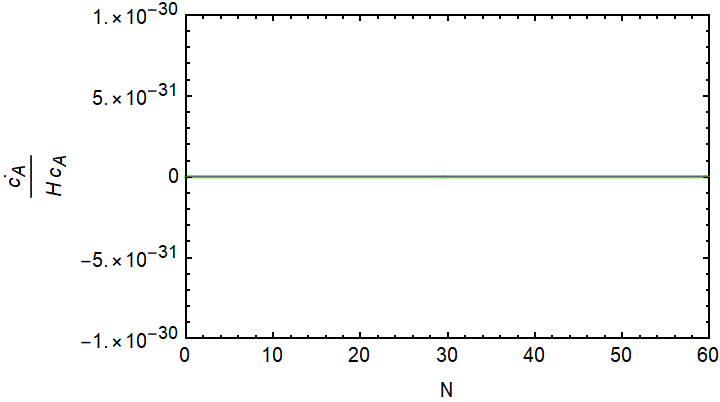
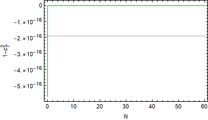
Also the adiabaticity constraint is satisfied for the whole duration of the inflationary era. This can be seen in Fig. 1 where we present the behavior of the constraint as a function of the -foldings number (left plot) and the gravitational wave speed as a function of the -foldings (right plot). As it can be seen, the resulting theory is phenomenologically viable and it also produces adiabatic perturbations, for the whole inflationary era. The numerical values of are too small, so we quote here the actual values at the end and the beginning of inflation and these are and respectively.
Now let us proceed with a model that is both ACT and Planck compatible, in which case the scalar potential is chosen as follows,
| (78) |
and in this case is,
| (79) |
and the first slow-roll index is,
| (80) |
while the -foldings number is,
| (81) |
This model can be compatible with both the ACT data and the Planck data as we now evince, for various choices of the free parameters of the model. For example the compatibility with the ACT data comes for the choice and , in which case we get , and the gravitational wave speed is and also the amplitude of the scalar perturbations is . With regard to the compatibility of the model with respect to the Planck data, the compatibility with the Planck data comes for the choice and , in which case we get , and the gravitational wave speed is and also the amplitude of the scalar perturbations is .
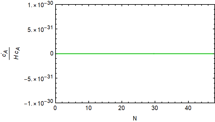
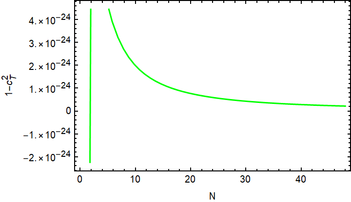
Also the adiabaticity constraint is satisfied for the whole duration of the inflationary era. This can be seen in Fig. 2 where we present the behavior of the constraint as a function of the -foldings number (left plot) and the gravitational wave speed as a function of the -foldings (right plot). As it can be seen, the resulting theory is phenomenologically viable and it also produces adiabatic perturbations, for the whole inflationary era. The numerical values of are too small, so we quote here the actual values at the end and the beginning of inflation and these are and respectively, using the Planck data compatibility. The same viability applies for the ACT data too.
Now let us proceed with a model that is ACT compatible only, in which case the scalar potential is chosen as follows,
| (82) |
and in this case is,
| (83) |
and the first slow-roll index is,
| (84) |
while the -foldings number is,
| (85) |
This model can be compatible wit the ACT data only as we now evince, for various choices of the free parameters of the model. For example the compatibility with the ACT data comes for the choice and , in which case we get , and the gravitational wave speed is and also the amplitude of the scalar perturbations is .
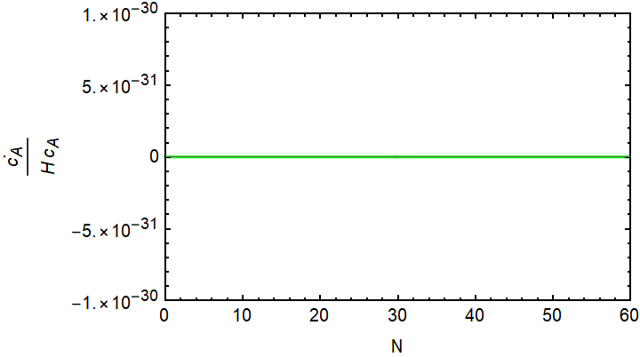
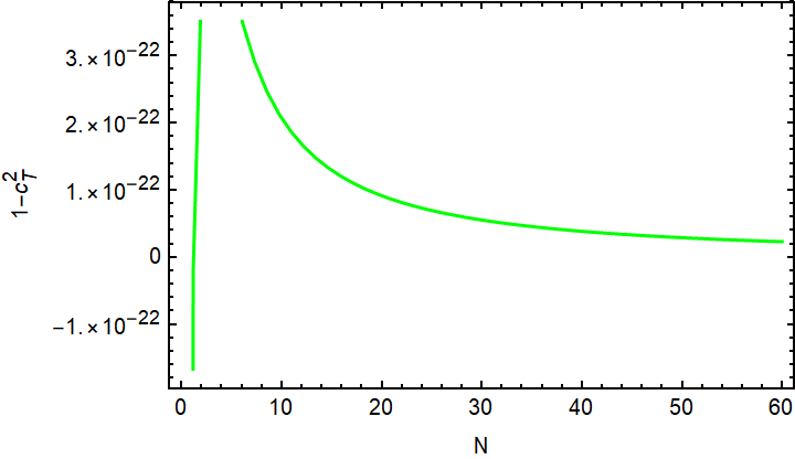
Also the adiabaticity constraint is satisfied for the whole duration of the inflationary era. This can be seen in Fig. 3 where we present the behavior of the constraint as a function of the -foldings number (left plot) and the gravitational wave speed as a function of the -foldings (right plot). As it can be seen, the resulting theory is phenomenologically viable and it also produces adiabatic perturbations, for the whole inflationary era. The numerical values of are too small, so we quote here the actual values at the end and the beginning of inflation and these are and respectively.
Now let us proceed with a model that is only ACT compatible, in which case the scalar potential is chosen as follows,
| (86) |
and in this case is,
| (87) |
and the first slow-roll index is,
| (88) |
while the -foldings number is,
| (89) |
This model can be compatible with the ACT data as we now evince, for various choices of the free parameters of the model. For example the compatibility with the ACT data comes for the choice and , in which case we get , and the gravitational wave speed is and also the amplitude of the scalar perturbations is .
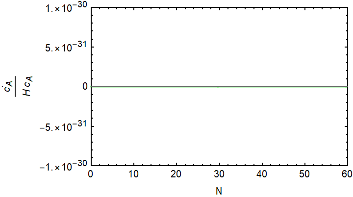
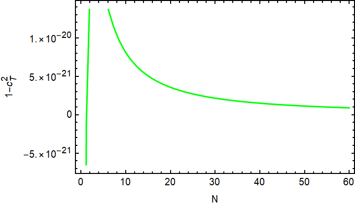
Also the adiabaticity constraint is satisfied for the whole duration of the inflationary era. This can be seen in Fig. 4 where we present the behavior of the constraint as a function of the -foldings number (left plot) and the gravitational wave speed as a function of the -foldings (right plot). As it can be seen, the resulting theory is phenomenologically viable and it also produces adiabatic perturbations, for the whole inflationary era. The numerical values of are too small, so we quote here the actual values at the end and the beginning of inflation and these are and respectively.
Now let us proceed with a model that is ACT only compatible, in which case the scalar potential is chosen as follows,
| (90) |
and in this case is,
| (91) |
and the first slow-roll index is,
| (92) |
while the -foldings number is,
| (93) |
This model can be compatible with the ACT data only as we now evince, for various choices of the free parameters of the model. For example the compatibility with the ACT data comes for the choice and , in which case we get , and the gravitational wave speed is and also the amplitude of the scalar perturbations is .
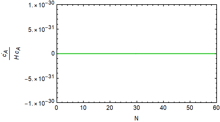
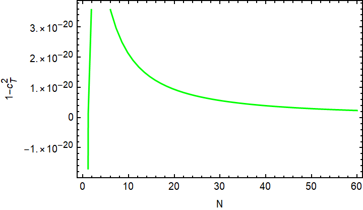
Also the adiabaticity constraint is satisfied for the whole duration of the inflationary era. This can be seen in Fig. 5 where we present the behavior of the constraint as a function of the -foldings number (left plot) and the gravitational wave speed as a function of the -foldings (right plot). As it can be seen, the resulting theory is phenomenologically viable and it also produces adiabatic perturbations, for the whole inflationary era. The numerical values of are too small, so we quote here the actual values at the end and the beginning of inflation and these are and respectively.
Finally we present another model that is both ACT and Planck compatible, in which case the scalar potential is chosen as follows,
| (94) |
and in this case is,
| (95) |
and the first slow-roll index is,
| (96) |
while the -foldings number is,
| (97) |
This model can be compatible with both the ACT data and the Planck data as we now evince, for various choices of the free parameters of the model. For example the compatibility with the ACT data comes for the choice and , in which case we get , and the gravitational wave speed is and also the amplitude of the scalar perturbations is . With regard to the compatibility of the model with respect to the Planck data, the compatibility with the Planck data comes for the choice and , in which case we get , and the gravitational wave speed is and also the amplitude of the scalar perturbations is .
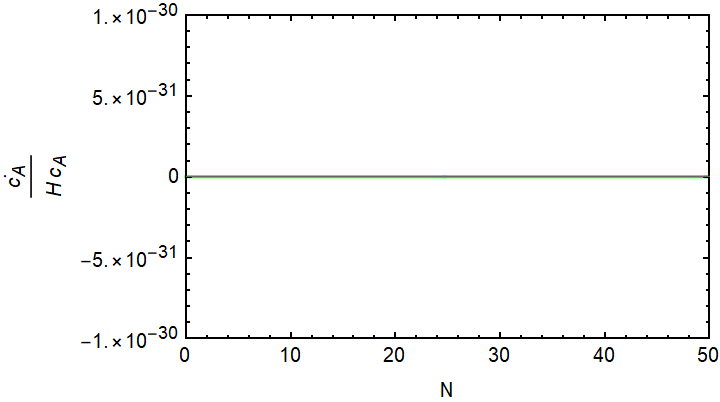
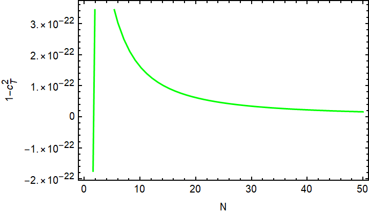
Also the adiabaticity constraint is satisfied for the whole duration of the inflationary era. This can be seen in Fig. 6 where we present the behavior of the constraint as a function of the -foldings number (left plot) and the gravitational wave speed as a function of the -foldings (right plot). As it can be seen, the resulting theory is phenomenologically viable and it also produces adiabatic perturbations, for the whole inflationary era. The numerical values of are too small, so we quote here the actual values at the end and the beginning of inflation and these are and respectively, by taking the Planck compatibility values of the free parameters.
IV Constrained EGB Theories, Non-Adiabaticity, Particle Production and New Features: Sinusoidal Power-Spectrum
There is a second formalism to obtain a viable inflationary EGB theory which is compatible with the GW170817 event, and it was developed in Refs. [72, 73, 74]. In the context of this formalism, one utilizes the fact that the gravitational wave speed of Eq. (16) is equal to unity when , and this happens when . This constraint on the Gauss-Bonnet coupling can be expressed in terms of the scalar field as follows,
| (98) |
where the “prime” indicates differentiation with respect to the scalar field. By assuming,
| (99) |
which is motivated by the scalar field slow-roll conditions, Eq. (98) takes the form,
| (100) |
| (101) |
We focus on models that further satisfy the following,
| (102) |
and in addition,
| (103) |
which is strongly related to the constraint (102). Eqs. (100) and (103), yield,
| (104) |
| (105) |
| (106) |
Also Eqs. (104) and (103) yield,
| (107) |
Thus the scalar field potential and the Gauss-Bonnet coupling are not free to choose in this context, but these satisfy,
| (108) |
So the slow-roll indices in this class of models take the form,
| (109) |
| (110) |
| (111) |
| (112) |
| (113) |
| (114) |
where, and is,
| (115) |
Hence the observational indices of inflation in this scenario are,
| (116) |
regarding the scalar spectral index, while the tensor spectral index and the tensor-to-scalar ratio acquire very simple forms,
| (117) |
| (118) |
Also the -foldings number takes the form,
| (119) |
The phenomenology of such framework was thoroughly analyzed in Refs. [72, 73, 74], so let us consider a viable model that is both ACT and Planck compatible, also considering the adiabaticity constraints.
Let us consider the model with scalar Gauss-Bonnet coupling function,
| (120) |
where is some dimensionless constant and . Combining (120) and Eq. (108) we obtain,
| (121) |
where is some dimensionless integration constant. Then we get,
| (122) |
| (123) |
| (124) |
| (125) |
| (126) |
| (127) |
So upon solving we get , and by solving Eq. (119) with respect to the variable we obtain . Hence the scalar spectral index takes the form,
| (128) |
and also the tensor-to-scalar ratio becomes,
| (129) |
In addition, the tensor-spectral index takes the form,
| (130) |
A viable set of parameter values that yields compatibility with the ACT data is ( for , for which , , and all these observables are compatible with the ACT constraints and the updated Planck tensor-to-scalar ratio constraints. For these values, the amplitude of the scalar perturbations is which is of course by construction, compatible with the Planck 2018 constraints [88]. Regarding the Planck data constraints, by choosing , we get, and and .
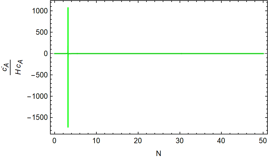
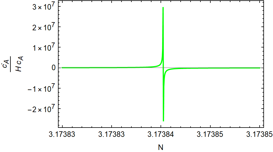
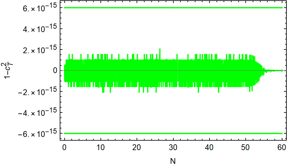
Also the adiabaticity constraint is satisfied for the largest part of the inflationary era, but it is strongly violated in the last few -foldings. Indeed, some characteristic values are at the end of inflation, at the beginning of inflation and for . Hence we need a closer look on the behavior of the adiabaticity condition , so in Fig. 7 we present the behavior of the constraint as a function of the -foldings number in both left and right upper plots. The right plot is a close up of the left plot, for small -foldings number. As it can be seen, the theory violates the adiabaticity constraints in the last few -foldings. In the bottom plot of Fig. 7 we present the behavior of the gravitational wave speed as a function of the -foldings, including the upper and lower limits of the GW170817 constraints. As it can be seen, the gravitational wave constraints are well respected.
Since the theory becomes non-adiabatic, interesting phenomena are expected, so let us first analyze possible reasons why this unexpected non-adiabaticity occurs for this theoretical framework. Using the analytic form of the sound wave speed for EGB in Eq. (20), we end up to the following expression,
| (131) |
Using the definition of the first slow-roll index,
| (132) |
the above expression (131) can be rewritten as follows,
| (133) |
therefore giving a rough estimate, the condition for adiabaticity of the scalar perturbations in EGB is,
| (134) |
Notice that enters in the field equation and thus the condition is an effective field theory requirement. Before proceeding, let us here reveal an important feature regarding the adiabaticity criteria. The requirement , contributes to the adiabaticity criterion (134), and can be written as,
| (135) |
where the “prime” denotes here differentiation with respect to the scalar field. In view of Eq. (135), the adiabaticity requirement reads,
| (136) |
therefore, in order to have adiabatic perturbations, one must have simultaneously,
| (137) |
The condition can be automatically satisfied if with , and such tracking conditions have been used in the literature [152] and it produces analytic solutions for inflation in single scalar field theory. A simple extension of the tracking condition in the context of EGB can therefore produce automatically adiabatic perturbations, if and , with the later being simply a slow-roll condition on the scalar field.
Now in the present context we have by construction, so the adiabaticity condition in Eq. (137) might be violated due to this and the relative fraction . This is probably the source of the non-adiabaticity of this framework, but note that the conditions (137) are not sufficient to determine the adiabaticity of the theory. Only the numerical study appearing in Fig. 7 provides enough and solid details on the problem of adiabaticity.
Now, since the theory becomes non-adiabatic at the end of inflation, interesting phenomena may occur at the end of inflation. The adiabaticity conditions are violated at the end of the inflationary regime and in fact in the very last few -foldings, so at the end of the inflationary regime, the Bogoliubov coefficient in Eq. (59) will increase, leading to particle production at the end of the inflationary regime. The energy density of these particles will be,
| (138) |
so by considering only the subhorizon modes that nearly exit the horizon at the end of inflation, we have , and since for all the models we analyzed, the final energy density of the produced particles is,
| (139) |
These particles redshift as radiation, hence this particle production at the end of the inflationary era is a mechanism for preheating which will facilitate the reheating era. Hence, this class of EGB inflationary models may lead to particle production at the end of inflation which acts as a gravitational reheating mechanism. Note that for the non-adiabatic modes, the CMB is not affected, since the non-adiabatic modes exit the Hubble horizon at the end of inflation, nearly at . However, we may have some secondary gravitational wave effects, which we aim to further examine in a future work.
Let us reveal another interesting feature of this class of models, suppose that in the context of this section’s scenario, the inflationary regime commenced from a Bunch-Davies vacuum and the “out” state is given by Eq. (56). The power spectrum in this scenario is,
| (140) |
which can be written as follows,
| (141) |
or equivalently,
| (142) |
where . The Bogoliubov coefficients and satisfy,
| (143) |
so the power spectrum becomes,
| (144) |
where we used the unperturbed power spectrum of the Bunch-Davies vacuum . Hence the power spectrum of the scalar perturbations in this case is rendered an oscillating spectrum, which is also known to appear in the literature for exotic inflationary scenarios, see for example [153, 154, 155, 156, 157, 158, 159, 160, 161, 162, 163, 164, 165, 166, 167, 168, 169, 170, 171, 172, 173, 174, 175, 176, 177, 178, 179, 180, 181]. This is a new feature for the EGB inflationary theories, but note that this oscillating feature is acquired by the power spectrum only at the last few -foldings, so it surely does not affect the CMB modes, and is surely distinct from the scenarios [153, 154, 155, 156, 157, 158, 159, 160, 161, 162, 163, 164, 165, 166, 167, 168, 169, 170, 171, 172, 173, 174, 175, 176, 177, 178, 179, 180, 181], because in these references the oscillating feature occurs for the whole inflationary era and not for a few -foldings in the end of inflation. Now it would be interesting to check for secondary gravitational wave effects at the end of inflation, due to this oscillating behavior, and we aim to investigate this feature in a future work.
V Conclusions
In this work we considered the adiabaticity of the cosmological scalar and tensor perturbations of EGB theories of gravity. We discussed the quantitative effects of the adiabaticity conditions and how do these affect the quantities entering in the EGB Lagrangian. We considered two classes of inflationary EGB theories of gravity which are compatible with the current CMB experiments and are also compatible with the GW170817 event. In the first class, the resulting cosmological perturbations are adiabatic during inflation, save the few last -foldings, and this results to particle creation at the end of inflation and also the power spectrum is affected acquiring sinusoidal terms. Also this adiabaticity violation at the end of inflation generates particle creation and thus the preheating is facilitated in this model. The other class of EGB theories has adiabatic perturbations during the inflationary regime. An interesting observation regarding the adiabaticity criterion of EGB theories is that the adiabaticity of EGB theory can occur solely if . Such tracking conditions have been analyzed in the literature [152], so it would be intriguing to work such a scenario in some detail. We aim to address this topic in a future work.
In retrospect, from the two viable EGB theories we presented, the unconstrained EGB theories are more stable and free from adiabaticity pathologies. For these theories, the dark energy perspective would be quite interesting to address, since in the present context, in the unconstrained EGB theories, the scalar Gauss-Bonnet coupling function satisfies . Thus inflation in the this context starts when and when , thus as inflation ends, the Gauss-Bonnet coupling increases, hence the dark energy era will be affected by the increasing Gauss-Bonnet coupling function . We aim to work along this research line in the near future.
References
- [1] A. D. Linde, Lect. Notes Phys. 738 (2008) 1 [arXiv:0705.0164 [hep-th]].
- [2] A. D. Linde, Phys. Lett. B 108 (1982), 389-393 doi:10.1016/0370-2693(82)91219-9
- [3] D. S. Gorbunov and V. A. Rubakov, “Introduction to the theory of the early universe: Cosmological perturbations and inflationary theory,” Hackensack, USA: World Scientific (2011) 489 p;
- [4] A. Linde, arXiv:1402.0526 [hep-th];
- [5] D. H. Lyth and A. Riotto, Phys. Rept. 314 (1999) 1 [hep-ph/9807278].
- [6] S. D. Odintsov, V. K. Oikonomou, I. Giannakoudi, F. P. Fronimos and E. C. Lymperiadou, Symmetry 15 (2023) no.9, 1701 doi:10.3390/sym15091701 [arXiv:2307.16308 [gr-qc]].
- [7] M. H. Abitbol et al. [Simons Observatory], Bull. Am. Astron. Soc. 51 (2019), 147 [arXiv:1907.08284 [astro-ph.IM]].
- [8] E. Allys et al. [LiteBIRD], PTEP 2023 (2023) no.4, 042F01 doi:10.1093/ptep/ptac150 [arXiv:2202.02773 [astro-ph.IM]].
- [9] S. Hild, M. Abernathy, F. Acernese, P. Amaro-Seoane, N. Andersson, K. Arun, F. Barone, B. Barr, M. Barsuglia and M. Beker, et al. Class. Quant. Grav. 28 (2011), 094013 doi:10.1088/0264-9381/28/9/094013 [arXiv:1012.0908 [gr-qc]].
- [10] J. Baker, J. Bellovary, P. L. Bender, E. Berti, R. Caldwell, J. Camp, J. W. Conklin, N. Cornish, C. Cutler and R. DeRosa, et al. [arXiv:1907.06482 [astro-ph.IM]].
- [11] T. L. Smith and R. Caldwell, Phys. Rev. D 100 (2019) no.10, 104055 doi:10.1103/PhysRevD.100.104055 [arXiv:1908.00546 [astro-ph.CO]].
- [12] J. Crowder and N. J. Cornish, Phys. Rev. D 72 (2005), 083005 doi:10.1103/PhysRevD.72.083005 [arXiv:gr-qc/0506015 [gr-qc]].
- [13] T. L. Smith and R. Caldwell, Phys. Rev. D 95 (2017) no.4, 044036 doi:10.1103/PhysRevD.95.044036 [arXiv:1609.05901 [gr-qc]].
- [14] N. Seto, S. Kawamura and T. Nakamura, Phys. Rev. Lett. 87 (2001), 221103 doi:10.1103/PhysRevLett.87.221103 [arXiv:astro-ph/0108011 [astro-ph]].
- [15] S. Kawamura, M. Ando, N. Seto, S. Sato, M. Musha, I. Kawano, J. Yokoyama, T. Tanaka, K. Ioka and T. Akutsu, et al. [arXiv:2006.13545 [gr-qc]].
- [16] A. Weltman, P. Bull, S. Camera, K. Kelley, H. Padmanabhan, J. Pritchard, A. Raccanelli, S. Riemer-Sørensen, L. Shao and S. Andrianomena, et al. Publ. Astron. Soc. Austral. 37 (2020), e002 doi:10.1017/pasa.2019.42 [arXiv:1810.02680 [astro-ph.CO]].
- [17] P. Auclair et al. [LISA Cosmology Working Group], [arXiv:2204.05434 [astro-ph.CO]].
- [18] G. Agazie et al. [NANOGrav], Astrophys. J. Lett. 951 (2023) no.1, L8 doi:10.3847/2041-8213/acdac6 [arXiv:2306.16213 [astro-ph.HE]].
- [19] S. Vagnozzi, JHEAp 39 (2023), 81-98 doi:10.1016/j.jheap.2023.07.001 [arXiv:2306.16912 [astro-ph.CO]].
- [20] V. K. Oikonomou, Phys. Rev. D 108 (2023) no.4, 043516 doi:10.1103/PhysRevD.108.043516 [arXiv:2306.17351 [astro-ph.CO]].
- [21] S. Nojiri, S. D. Odintsov and V. K. Oikonomou, Phys. Rept. 692 (2017) 1 [arXiv:1705.11098 [gr-qc]].
-
[22]
S. Capozziello, M. De Laurentis,
Phys. Rept. 509, 167 (2011);
V. Faraoni and S. Capozziello, Fundam. Theor. Phys. 170 (2010). - [23] S. Nojiri, S.D. Odintsov, Phys. Rept. 505, 59 (2011);
- [24] S. Nojiri and S. D. Odintsov, Phys. Rev. D 68 (2003), 123512 doi:10.1103/PhysRevD.68.123512 [arXiv:hep-th/0307288 [hep-th]].
- [25] S. Capozziello, V. F. Cardone and A. Troisi, Phys. Rev. D 71 (2005), 043503 doi:10.1103/PhysRevD.71.043503 [arXiv:astro-ph/0501426 [astro-ph]].
- [26] S. Capozziello, C. A. Mantica and L. G. Molinari, Int. J. Geom. Meth. Mod. Phys. 16 (2018) no.01, 1950008 doi:10.1142/S0219887819500087 [arXiv:1810.03204 [gr-qc]].
- [27] S. Capozziello, V. F. Cardone and M. Francaviglia, Gen. Rel. Grav. 38 (2006), 711-734 doi:10.1007/s10714-006-0261-x [arXiv:astro-ph/0410135 [astro-ph]].
- [28] J. c. Hwang and H. Noh, Phys. Lett. B 506 (2001), 13-19 doi:10.1016/S0370-2693(01)00404-X [arXiv:astro-ph/0102423 [astro-ph]].
- [29] K. Bamba, G. Cognola, S. D. Odintsov and S. Zerbini, Phys. Rev. D 90 (2014) no.2, 023525 doi:10.1103/PhysRevD.90.023525 [arXiv:1404.4311 [gr-qc]].
- [30] S. Nojiri and S. D. Odintsov, Phys. Rev. D 74 (2006), 086005 doi:10.1103/PhysRevD.74.086005 [arXiv:hep-th/0608008 [hep-th]].
- [31] Y. S. Song, W. Hu and I. Sawicki, Phys. Rev. D 75 (2007), 044004 doi:10.1103/PhysRevD.75.044004 [arXiv:astro-ph/0610532 [astro-ph]].
- [32] S. Capozziello, V. F. Cardone and V. Salzano, Phys. Rev. D 78 (2008), 063504 doi:10.1103/PhysRevD.78.063504 [arXiv:0802.1583 [astro-ph]].
- [33] R. Bean, D. Bernat, L. Pogosian, A. Silvestri and M. Trodden, Phys. Rev. D 75 (2007), 064020 doi:10.1103/PhysRevD.75.064020 [arXiv:astro-ph/0611321 [astro-ph]].
- [34] S. Capozziello and M. De Laurentis, Annalen Phys. 524 (2012), 545-578 doi:10.1002/andp.201200109
- [35] T. Faulkner, M. Tegmark, E. F. Bunn and Y. Mao, Phys. Rev. D 76 (2007), 063505 doi:10.1103/PhysRevD.76.063505 [arXiv:astro-ph/0612569 [astro-ph]].
- [36] G. J. Olmo, Phys. Rev. D 75 (2007), 023511 doi:10.1103/PhysRevD.75.023511 [arXiv:gr-qc/0612047 [gr-qc]].
- [37] I. Sawicki and W. Hu, Phys. Rev. D 75 (2007), 127502 doi:10.1103/PhysRevD.75.127502 [arXiv:astro-ph/0702278 [astro-ph]].
- [38] V. Faraoni, Phys. Rev. D 75 (2007), 067302 doi:10.1103/PhysRevD.75.067302 [arXiv:gr-qc/0703044 [gr-qc]].
- [39] S. Carloni, P. K. S. Dunsby and A. Troisi, Phys. Rev. D 77 (2008), 024024 doi:10.1103/PhysRevD.77.024024 [arXiv:0707.0106 [gr-qc]].
- [40] S. Nojiri and S. D. Odintsov, Phys. Lett. B 657 (2007), 238-245 doi:10.1016/j.physletb.2007.10.027 [arXiv:0707.1941 [hep-th]].
- [41] S. Capozziello, A. Stabile and A. Troisi, Phys. Rev. D 76 (2007), 104019 doi:10.1103/PhysRevD.76.104019 [arXiv:0708.0723 [gr-qc]].
- [42] N. Deruelle, M. Sasaki and Y. Sendouda, Prog. Theor. Phys. 119 (2008), 237-251 doi:10.1143/PTP.119.237 [arXiv:0711.1150 [gr-qc]].
- [43] S. A. Appleby and R. A. Battye, JCAP 05 (2008), 019 doi:10.1088/1475-7516/2008/05/019 [arXiv:0803.1081 [astro-ph]].
- [44] P. K. S. Dunsby, E. Elizalde, R. Goswami, S. Odintsov and D. S. Gomez, Phys. Rev. D 82 (2010), 023519 doi:10.1103/PhysRevD.82.023519 [arXiv:1005.2205 [gr-qc]].
- [45] V. K. Oikonomou, Phys. Rev. D 103 (2021) no.12, 124028 doi:10.1103/PhysRevD.103.124028 [arXiv:2012.01312 [gr-qc]].
- [46] V. K. Oikonomou, Phys. Rev. D 103 (2021) no.4, 044036 doi:10.1103/PhysRevD.103.044036 [arXiv:2012.00586 [astro-ph.CO]].
- [47] J. c. Hwang and H. Noh, Phys. Rev. D 71 (2005) 063536 doi:10.1103/PhysRevD.71.063536 [gr-qc/0412126].
- [48] G. Cognola, E. Elizalde, S. Nojiri, S. Odintsov and S. Zerbini, Phys. Rev. D 75 (2007) 086002 doi:10.1103/PhysRevD.75.086002 [hep-th/0611198].
- [49] S. Nojiri, S. D. Odintsov and M. Sasaki, Phys. Rev. D 71 (2005) 123509 doi:10.1103/PhysRevD.71.123509 [hep-th/0504052].
- [50] S. Nojiri and S. D. Odintsov, Phys. Lett. B 631 (2005) 1 doi:10.1016/j.physletb.2005.10.010 [hep-th/0508049].
- [51] M. Satoh, S. Kanno and J. Soda, Phys. Rev. D 77 (2008) 023526 doi:10.1103/PhysRevD.77.023526 [arXiv:0706.3585 [astro-ph]].
- [52] Z. Yi, Y. Gong and M. Sabir, Phys. Rev. D 98 (2018) no.8, 083521 doi:10.1103/PhysRevD.98.083521 [arXiv:1804.09116 [gr-qc]].
- [53] Z. K. Guo and D. J. Schwarz, Phys. Rev. D 80 (2009) 063523 doi:10.1103/PhysRevD.80.063523 [arXiv:0907.0427 [hep-th]].
- [54] Z. K. Guo and D. J. Schwarz, Phys. Rev. D 81 (2010) 123520 doi:10.1103/PhysRevD.81.123520 [arXiv:1001.1897 [hep-th]].
- [55] P. X. Jiang, J. W. Hu and Z. K. Guo, Phys. Rev. D 88 (2013) 123508 doi:10.1103/PhysRevD.88.123508 [arXiv:1310.5579 [hep-th]].
- [56] C. van de Bruck, K. Dimopoulos, C. Longden and C. Owen, arXiv:1707.06839 [astro-ph.CO].
- [57] E. O. Pozdeeva, M. R. Gangopadhyay, M. Sami, A. V. Toporensky and S. Y. Vernov, Phys. Rev. D 102 (2020) no.4, 043525 doi:10.1103/PhysRevD.102.043525 [arXiv:2006.08027 [gr-qc]].
- [58] S. Vernov and E. Pozdeeva, Universe 7 (2021) no.5, 149 doi:10.3390/universe7050149 [arXiv:2104.11111 [gr-qc]].
- [59] E. O. Pozdeeva and S. Y. Vernov, Eur. Phys. J. C 81 (2021) no.7, 633 doi:10.1140/epjc/s10052-021-09435-8 [arXiv:2104.04995 [gr-qc]].
- [60] I. Fomin, Eur. Phys. J. C 80 (2020) no.12, 1145 doi:10.1140/epjc/s10052-020-08718-w [arXiv:2004.08065 [gr-qc]].
- [61] M. De Laurentis, M. Paolella and S. Capozziello, Phys. Rev. D 91 (2015) no.8, 083531 doi:10.1103/PhysRevD.91.083531 [arXiv:1503.04659 [gr-qc]].
-
[62]
Scalar Field Cosmology, S. Chervon, I. Fomin, V. Yurov and
A. Yurov, World Scientific 2019,
doi:10.1142/11405 - [63] K. Nozari and N. Rashidi, Phys. Rev. D 95 (2017) no.12, 123518 doi:10.1103/PhysRevD.95.123518 [arXiv:1705.02617 [astro-ph.CO]].
- [64] S. D. Odintsov and V. K. Oikonomou, Phys. Rev. D 98 (2018) no.4, 044039 doi:10.1103/PhysRevD.98.044039 [arXiv:1808.05045 [gr-qc]].
- [65] S. Kawai, M. a. Sakagami and J. Soda, Phys. Lett. B 437, 284 (1998) doi:10.1016/S0370-2693(98)00925-3 [gr-qc/9802033].
- [66] Z. Yi and Y. Gong, Universe 5 (2019) no.9, 200 doi:10.3390/universe5090200 [arXiv:1811.01625 [gr-qc]].
- [67] C. van de Bruck, K. Dimopoulos and C. Longden, Phys. Rev. D 94 (2016) no.2, 023506 doi:10.1103/PhysRevD.94.023506 [arXiv:1605.06350 [astro-ph.CO]].
- [68] K. i. Maeda, N. Ohta and R. Wakebe, Eur. Phys. J. C 72 (2012) 1949 doi:10.1140/epjc/s10052-012-1949-6 [arXiv:1111.3251 [hep-th]].
- [69] W. Y. Ai, Commun. Theor. Phys. 72 (2020) no.9, 095402 doi:10.1088/1572-9494/aba242 [arXiv:2004.02858 [gr-qc]].
- [70] R. Easther and K. i. Maeda, Phys. Rev. D 54 (1996) 7252 doi:10.1103/PhysRevD.54.7252 [hep-th/9605173].
- [71] A. Codello and R. K. Jain, Class. Quant. Grav. 33 (2016) no.22, 225006 doi:10.1088/0264-9381/33/22/225006 [arXiv:1507.06308 [gr-qc]].
- [72] V. K. Oikonomou, Class. Quant. Grav. 38 (2021) no.19, 195025 doi:10.1088/1361-6382/ac2168 [arXiv:2108.10460 [gr-qc]].
- [73] V. K. Oikonomou, Astropart. Phys. 141 (2022), 102718 doi:10.1016/j.astropartphys.2022.102718 [arXiv:2204.06304 [gr-qc]].
- [74] S. D. Odintsov, V. K. Oikonomou and F. P. Fronimos, Nucl. Phys. B 958 (2020), 115135 doi:10.1016/j.nuclphysb.2020.115135 [arXiv:2003.13724 [gr-qc]].
- [75] V. K. Oikonomou, Phys. Lett. B 856 (2024), 138890 doi:10.1016/j.physletb.2024.138890 [arXiv:2407.12155 [gr-qc]].
- [76] J. Fier, H. Han, B. Li, K. Lin, S. Mukohyama and A. Wang, [arXiv:2503.01975 [gr-qc]].
- [77] E. O. Pozdeeva, M. A. Skugoreva, A. V. Toporensky and S. Y. Vernov, JCAP 09 (2024), 050 doi:10.1088/1475-7516/2024/09/050 [arXiv:2403.06147 [gr-qc]].
- [78] S. D. Odintsov, V. K. Oikonomou, P. Tsyba, O. Razina and D. Rakhatov, [arXiv:2604.18861 [gr-qc]].
- [79] B. P. Abbott et al. [LIGO Scientific and Virgo], Phys. Rev. Lett. 119 (2017) no.16, 161101 doi:10.1103/PhysRevLett.119.161101 [arXiv:1710.05832 [gr-qc]].
- [80] B. P. Abbott et al. [LIGO Scientific, Virgo, Fermi-GBM and INTEGRAL], Astrophys. J. Lett. 848 (2017) no.2, L13 doi:10.3847/2041-8213/aa920c [arXiv:1710.05834 [astro-ph.HE]].
- [81] B. P. Abbott et al. “Multi-messenger Observations of a Binary Neutron Star Merger,” Astrophys. J. 848 (2017) no.2, L12 doi:10.3847/2041-8213/aa91c9 [arXiv:1710.05833 [astro-ph.HE]].
- [82] B. P. Abbott et al. [LIGO Scientific and Virgo], Phys. Rev. D 100 (2019) no.6, 061101 doi:10.1103/PhysRevD.100.061101 [arXiv:1903.02886 [gr-qc]].
- [83] J. M. Ezquiaga and M. Zumalacárregui, Phys. Rev. Lett. 119 (2017) no.25, 251304 doi:10.1103/PhysRevLett.119.251304 [arXiv:1710.05901 [astro-ph.CO]].
- [84] T. Baker, E. Bellini, P. G. Ferreira, M. Lagos, J. Noller and I. Sawicki, Phys. Rev. Lett. 119 (2017) no.25, 251301 doi:10.1103/PhysRevLett.119.251301 [arXiv:1710.06394 [astro-ph.CO]].
- [85] P. Creminelli and F. Vernizzi, Phys. Rev. Lett. 119 (2017) no.25, 251302 doi:10.1103/PhysRevLett.119.251302 [arXiv:1710.05877 [astro-ph.CO]].
- [86] J. Sakstein and B. Jain, Phys. Rev. Lett. 119 (2017) no.25, 251303 doi:10.1103/PhysRevLett.119.251303 [arXiv:1710.05893 [astro-ph.CO]].
- [87] S. Boran, S. Desai, E. O. Kahya and R. P. Woodard, Phys. Rev. D 97 (2018) no.4, 041501 doi:10.1103/PhysRevD.97.041501 [arXiv:1710.06168 [astro-ph.HE]].
- [88] Y. Akrami et al. [Planck], Astron. Astrophys. 641 (2020), A10 doi:10.1051/0004-6361/201833887 [arXiv:1807.06211 [astro-ph.CO]].
- [89] P. A. R. Ade et al. [BICEP and Keck], Phys. Rev. Lett. 127 (2021) no.15, 151301 doi:10.1103/PhysRevLett.127.151301 [arXiv:2110.00483 [astro-ph.CO]].
- [90] T. Louis et al. [ACT], [arXiv:2503.14452 [astro-ph.CO]].
- [91] E. Calabrese et al. [ACT], [arXiv:2503.14454 [astro-ph.CO]].
- [92] R. Kallosh, A. Linde and D. Roest, [arXiv:2503.21030 [hep-th]].
- [93] Q. Gao, Y. Gong, Z. Yi and F. Zhang, [arXiv:2504.15218 [astro-ph.CO]].
- [94] L. Liu, Z. Yi and Y. Gong, [arXiv:2505.02407 [astro-ph.CO]].
- [95] Yogesh, A. Mohammadi, Q. Wu and T. Zhu, [arXiv:2505.05363 [astro-ph.CO]].
- [96] Z. Yi, X. Wang, Q. Gao and Y. Gong, [arXiv:2505.10268 [astro-ph.CO]].
- [97] Z. Z. Peng, Z. C. Chen and L. Liu, [arXiv:2505.12816 [astro-ph.CO]].
- [98] W. Yin, [arXiv:2505.03004 [hep-ph]].
- [99] C. T. Byrnes, M. Cortês and A. R. Liddle, [arXiv:2505.09682 [astro-ph.CO]].
- [100] W. J. Wolf, [arXiv:2506.12436 [astro-ph.CO]].
- [101] S. Aoki, H. Otsuka and R. Yanagita, [arXiv:2504.01622 [hep-ph]].
- [102] Q. Gao, Y. Qian, Y. Gong and Z. Yi, [arXiv:2506.18456 [gr-qc]].
- [103] M. Zahoor, S. Khan and I. A. Bhat, [arXiv:2507.18684 [astro-ph.CO]].
- [104] E. G. M. Ferreira, E. McDonough, L. Balkenhol, R. Kallosh, L. Knox and A. Linde, [arXiv:2507.12459 [astro-ph.CO]].
- [105] A. Mohammadi, Yogesh and A. Wang, [arXiv:2507.06544 [astro-ph.CO]].
- [106] S. Choudhury, G. Bauyrzhan, S. K. Singh and K. Yerzhanov, [arXiv:2506.15407 [astro-ph.CO]].
- [107] S. D. Odintsov and V. K. Oikonomou, Phys. Lett. B 868 (2025), 139779 doi:10.1016/j.physletb.2025.139779 [arXiv:2506.08193 [gr-qc]].
- [108] R. D. A. Q., J. Chagoya and A. A. Roque, [arXiv:2508.13273 [gr-qc]].
- [109] Y. Zhu, Q. Gao, Y. Gong and Z. Yi, [arXiv:2508.09707 [astro-ph.CO]].
- [110] G. Kouniatalis and E. N. Saridakis, [arXiv:2507.17721 [astro-ph.CO]].
- [111] M. Hai, A. R. Kamal, N. F. Shamma and M. S. J. Shuvo, [arXiv:2506.08083 [hep-th]].
- [112] C. Dioguardi, A. J. Iovino and A. Racioppi, Phys. Lett. B 868 (2025), 139664 doi:10.1016/j.physletb.2025.139664 [arXiv:2504.02809 [gr-qc]].
- [113] J. Yuennan, P. Koad, F. Atamurotov and P. Channuie, [arXiv:2508.17263 [astro-ph.CO]].
- [114] H. J. Kuralkar, S. Panda and A. Vidyarthi, [arXiv:2504.15061 [gr-qc]].
- [115] H. J. Kuralkar, S. Panda and A. Vidyarthi, JCAP 05 (2025), 073 doi:10.1088/1475-7516/2025/05/073 [arXiv:2502.03573 [astro-ph.CO]].
- [116] T. Modak, [arXiv:2509.02979 [astro-ph.CO]].
- [117] S. Aoki, H. Otsuka and R. Yanagita, [arXiv:2509.06739 [hep-ph]].
- [118] Z. Ahghari and M. Farhoudi, [arXiv:2512.12286 [gr-qc]].
- [119] E. McDonough and E. G. M. Ferreira, [arXiv:2512.05108 [astro-ph.CO]].
- [120] D. Chakraborty, M. Hai, S. T. Jahan, A. R. Kamal and M. S. J. Shuvo, [arXiv:2511.19610 [hep-th]].
- [121] S. Noori Gashti, M. A. S. Afshar, M. R. Alipour, B. Pourhassan and J. Sadeghi, Eur. Phys. J. C 85 (2025) no.11, 1343 doi:10.1140/epjc/s10052-025-15066-0
- [122] J. Yuennan, F. Atamurotov and P. Channuie, [arXiv:2511.17216 [astro-ph.CO]].
- [123] B. Deb and A. Deshamukhya, [arXiv:2511.06453 [gr-qc]].
- [124] M. A. S. Afshar, S. Noori Gashti, M. R. Alipour, B. Pourhassan, I. Sakalli and J. Sadeghi, [arXiv:2510.20876 [astro-ph.CO]].
- [125] J. Ellis, M. A. G. Garcia, K. A. Olive and S. Verner, [arXiv:2510.18656 [hep-ph]].
- [126] L. Iacconi, S. Bhattacharya, M. Fasiello and D. Wands, [arXiv:2511.14673 [astro-ph.CO]].
- [127] J. Yuennan, F. Atamurotov and P. Channuie, Phys. Lett. B 872 (2026), 140065 doi:10.1016/j.physletb.2025.140065 [arXiv:2509.23329 [gr-qc]].
- [128] Q. Y. Wang, [arXiv:2512.10862 [astro-ph.CO]].
- [129] Z. C. Qiu, Y. H. Pang and Q. G. Huang, [arXiv:2510.18320 [astro-ph.CO]].
- [130] X. Wang, K. Kohri and T. T. Yanagida, [arXiv:2506.06797 [astro-ph.CO]].
- [131] T. Asaka, S. Iso, H. Kawai, K. Kohri, T. Noumi and T. Terada, PTEP 2016 (2016) no.12, 123E01 doi:10.1093/ptep/ptw161 [arXiv:1507.04344 [hep-th]].
- [132] V. K. Oikonomou, Phys. Lett. B 871 (2025), 139972 doi:10.1016/j.physletb.2025.139972 [arXiv:2508.17363 [gr-qc]].
- [133] S. Choudhury, S. K. Singh and S. K. Sahoo, [arXiv:2511.19898 [gr-qc]].
- [134] S. K. Singh, [arXiv:2511.05545 [hep-ph]].
- [135] J. Kim, X. Wang, Y. l. Zhang and Z. Ren, JCAP 09 (2025), 011 doi:10.1088/1475-7516/2025/09/011 [arXiv:2504.12035 [astro-ph.CO]].
- [136] Z. Y. Peng, H. S. Yuan, Q. Lai, J. Q. Jiang, G. Ye, J. Zhang and Y. S. Piao, [arXiv:2601.14288 [astro-ph.CO]].
- [137] Samson S. Hounmenou, Ines G. Salako, Biswajit Deb, Atri Deshamukhya, Annals Phys. 490 (2026) 170462 https://doi.org/10.1016/j.aop.2026.170462
- [138] S. D. Odintsov and V. K. Oikonomou, Phys. Lett. B 880 (2026), 140805 doi:10.1016/j.physletb.2026.140805 [arXiv:2605.17813 [gr-qc]].
- [139] A. G. Adame et al. [DESI], JCAP 04 (2025), 012 doi:10.1088/1475-7516/2025/04/012 [arXiv:2404.03000 [astro-ph.CO]].
- [140] D. H. Lee, W. Yang, E. Di Valentino, S. Pan and C. van de Bruck, [arXiv:2507.11432 [astro-ph.CO]].
- [141] E. Özülker, E. Di Valentino and W. Giarè, [arXiv:2506.19053 [astro-ph.CO]].
- [142] D. A. Kessler, L. A. Escamilla, S. Pan and E. Di Valentino, [arXiv:2504.00776 [astro-ph.CO]].
- [143] S. Nojiri, S. D. Odintsov and V. K. Oikonomou, [arXiv:2506.21010 [gr-qc]].
- [144] S. Vagnozzi, Phys. Rev. D 102 (2020) no.2, 023518 doi:10.1103/PhysRevD.102.023518 [arXiv:1907.07569 [astro-ph.CO]].
- [145] D. Pedrotti, J. Q. Jiang, L. A. Escamilla, S. S. da Costa and S. Vagnozzi, Phys. Rev. D 111 (2025) no.2, 023506 doi:10.1103/PhysRevD.111.023506 [arXiv:2408.04530 [astro-ph.CO]].
- [146] J. Q. Jiang, D. Pedrotti, S. S. da Costa and S. Vagnozzi, Phys. Rev. D 110 (2024) no.12, 123519 doi:10.1103/PhysRevD.110.123519 [arXiv:2408.02365 [astro-ph.CO]].
- [147] S. Vagnozzi, Universe 9 (2023) no.9, 393 doi:10.3390/universe9090393 [arXiv:2308.16628 [astro-ph.CO]].
- [148] S. A. Adil, Ö. Akarsu, E. Di Valentino, R. C. Nunes, E. Özülker, A. A. Sen and E. Specogna, Phys. Rev. D 109 (2024) no.2, 023527 doi:10.1103/PhysRevD.109.023527 [arXiv:2306.08046 [astro-ph.CO]].
- [149] A. Bernui, E. Di Valentino, W. Giarè, S. Kumar and R. C. Nunes, Phys. Rev. D 107 (2023) no.10, 103531 doi:10.1103/PhysRevD.107.103531 [arXiv:2301.06097 [astro-ph.CO]].
- [150] S. Gariazzo, E. Di Valentino, O. Mena and R. C. Nunes, Phys. Rev. D 106 (2022) no.2, 023530 doi:10.1103/PhysRevD.106.023530 [arXiv:2111.03152 [astro-ph.CO]].
- [151] M. A. Sabogal, A. J. Iovino and S. Vagnozzi, [arXiv:2606.31362 [astro-ph.CO]].
- [152] V. K. Oikonomou, [arXiv:2603.11794 [gr-qc]].
- [153] C. Zeng, E. D. Kovetz, X. Chen, Y. Gong, J. B. Muñoz and M. Kamionkowski, Phys. Rev. D 99 (2019) no.4, 043517 doi:10.1103/PhysRevD.99.043517 [arXiv:1812.05105 [astro-ph.CO]].
- [154] G. Domènech and M. Kamionkowski, JCAP 11 (2019), 040 doi:10.1088/1475-7516/2019/11/040 [arXiv:1905.04323 [astro-ph.CO]].
- [155] U. H. Danielsson, Phys. Rev. D 66 (2002), 023511 doi:10.1103/PhysRevD.66.023511 [arXiv:hep-th/0203198 [hep-th]].
- [156] M. G. Jackson and G. Shiu, Phys. Rev. D 88 (2013) no.12, 123511 doi:10.1103/PhysRevD.88.123511 [arXiv:1303.4973 [hep-th]].
- [157] A. Kempf, Phys. Rev. D 63 (2001), 083514 doi:10.1103/PhysRevD.63.083514 [arXiv:astro-ph/0009209 [astro-ph]].
- [158] R. Easther, B. R. Greene, W. H. Kinney and G. Shiu, Phys. Rev. D 67 (2003), 063508 doi:10.1103/PhysRevD.67.063508 [arXiv:hep-th/0110226 [hep-th]].
- [159] J. Martin and R. Brandenberger, Phys. Rev. D 68 (2003), 063513 doi:10.1103/PhysRevD.68.063513 [arXiv:hep-th/0305161 [hep-th]].
- [160] X. Chen, R. Easther and E. A. Lim, JCAP 04 (2008), 010 doi:10.1088/1475-7516/2008/04/010 [arXiv:0801.3295 [astro-ph]].
- [161] R. Flauger, L. McAllister, E. Pajer, A. Westphal and G. Xu, JCAP 06 (2010), 009 doi:10.1088/1475-7516/2010/06/009 [arXiv:0907.2916 [hep-th]].
- [162] L. Covi, J. Hamann, A. Melchiorri, A. Slosar and I. Sorbera, Phys. Rev. D 74 (2006), 083509 doi:10.1103/PhysRevD.74.083509 [arXiv:astro-ph/0606452 [astro-ph]].
- [163] J. Hamann, L. Covi, A. Melchiorri and A. Slosar, Phys. Rev. D 76 (2007), 023503 doi:10.1103/PhysRevD.76.023503 [arXiv:astro-ph/0701380 [astro-ph]].
- [164] D. K. Hazra, M. Aich, R. K. Jain, L. Sriramkumar and T. Souradeep, JCAP 10 (2010), 008 doi:10.1088/1475-7516/2010/10/008 [arXiv:1005.2175 [astro-ph.CO]].
- [165] A. Shafieloo and T. Souradeep, Phys. Rev. D 70 (2004), 043523 doi:10.1103/PhysRevD.70.043523 [arXiv:astro-ph/0312174 [astro-ph]].
- [166] A. Achúcarro, V. Atal, P. Ortiz and J. Torrado, Phys. Rev. D 89 (2014) no.10, 103006 doi:10.1103/PhysRevD.89.103006 [arXiv:1311.2552 [astro-ph.CO]].
- [167] D. K. Hazra, A. Shafieloo and T. Souradeep, JCAP 11 (2014), 011 doi:10.1088/1475-7516/2014/11/011 [arXiv:1406.4827 [astro-ph.CO]].
- [168] X. Chen, M. H. Namjoo and Y. Wang, JCAP 02 (2015), 027 doi:10.1088/1475-7516/2015/02/027 [arXiv:1411.2349 [astro-ph.CO]].
- [169] G. Nicholson and C. R. Contaldi, JCAP 07 (2009), 011 doi:10.1088/1475-7516/2009/07/011 [arXiv:0903.1106 [astro-ph.CO]].
- [170] P. Hunt and S. Sarkar, JCAP 12 (2015), 052 doi:10.1088/1475-7516/2015/12/052 [arXiv:1510.03338 [astro-ph.CO]].
- [171] M. Braglia, X. Chen and D. K. Hazra, JCAP 06 (2021), 005 doi:10.1088/1475-7516/2021/06/005 [arXiv:2103.03025 [astro-ph.CO]].
- [172] M. Braglia, X. Chen and D. K. Hazra, Eur. Phys. J. C 82 (2022) no.5, 498 doi:10.1140/epjc/s10052-022-10461-3 [arXiv:2106.07546 [astro-ph.CO]].
- [173] A. Antony and S. Jain, Eur. Phys. J. C 82 (2022) no.8, 687 doi:10.1140/epjc/s10052-022-10616-2 [arXiv:2110.06837 [astro-ph.CO]].
- [174] D. K. Hazra, A. Antony and A. Shafieloo, JCAP 08 (2022) no.08, 063 doi:10.1088/1475-7516/2022/08/063 [arXiv:2201.12000 [astro-ph.CO]].
- [175] A. Antony, F. Finelli, D. K. Hazra and A. Shafieloo, Phys. Rev. Lett. 130 (2023) no.11, 111001 doi:10.1103/PhysRevLett.130.111001 [arXiv:2202.14028 [astro-ph.CO]].
- [176] E. Silverstein and A. Westphal, Phys. Rev. D 78 (2008), 106003 doi:10.1103/PhysRevD.78.106003 [arXiv:0803.3085 [hep-th]].
- [177] L. McAllister, E. Silverstein and A. Westphal, Phys. Rev. D 82 (2010), 046003 doi:10.1103/PhysRevD.82.046003 [arXiv:0808.0706 [hep-th]].
- [178] S. R. Behbahani, A. Dymarsky, M. Mirbabayi and L. Senatore, JCAP 12 (2012), 036 doi:10.1088/1475-7516/2012/12/036 [arXiv:1111.3373 [hep-th]].
- [179] X. Wang, B. Feng, M. Li, X. L. Chen and X. Zhang, Int. J. Mod. Phys. D 14 (2005), 1347 doi:10.1142/S0218271805006985 [arXiv:astro-ph/0209242 [astro-ph]].
- [180] R. Easther, B. R. Greene, W. H. Kinney and G. Shiu, Phys. Rev. D 66 (2002), 023518 doi:10.1103/PhysRevD.66.023518 [arXiv:hep-th/0204129 [hep-th]].
- [181] V. Bozza, M. Giovannini and G. Veneziano, JCAP 05 (2003), 001 doi:10.1088/1475-7516/2003/05/001 [arXiv:hep-th/0302184 [hep-th]].