Mass Lumping and Numerical Quadrature for Approximation of Fractional Elliptic Differential Equations Driven by Gaussian White Noise††thanks: This publication is based upon work supported by King Abdullah University of Science and Technology (KAUST) under Award No. ORFS-CRG12-2024-6399.
Abstract
Fractional elliptic stochastic partial differential equations (SPDEs) are widely used in statistics and machine learning for computationally efficient and flexible modeling of Gaussian random fields. The computational efficiency of the SPDE approach relies on finite element approximations combined with numerical quadrature and mass lumping, which enable sparse matrix methods during inference. Although many works have studied finite element approximations of fractional SPDEs, the effect of the mass lumping and quadrature approximations used in practice has not been fully analyzed. To fill this gap, we derive convergence rates for numerical approximations of fractional SPDEs based on finite element discretizations combined with numerical quadrature and mass lumping. Specifically, we obtain explicit convergence rates for the mean-squared error of the covariance function in a general framework that covers the main settings where mass lumping is used in the SPDE approach. We also analyze non-stationary variance-control factors of the form , where is spatially varying, and derive covariance error estimates showing how the regularity of affects the convergence rate. As specific examples, we provide results for random fields on bounded Euclidean domains, Riemannian manifolds, and metric graphs. Numerical experiments are presented that confirm the theoretical results.
Keywords: Fractional SPDEs, Gaussian random fields, finite element methods, mass lumping, covariance approximation
MSC (2020): Primary 65N30, 65D32, 60H15, 35R11; Secondary 65D30, 62M30, 60G60
1 Introduction and Notation
1.1 Introduction
The stochastic partial differential equation (SPDE) approach [51] is widely used to represent Gaussian random fields in spatial statistics [50]. It considers Gaussian random fields on a domain that can be represented as solutions to SPDEs of the form
| (1.1) |
where is Gaussian white noise on , and is a fractional power of a second-order elliptic differential operator . The choice of determines the covariance structure of . A motivating example is the elliptic operator , where is a suitable matrix-valued function and is a real-valued function on . Here, and denote the gradient and divergence operators on the underlying spatial domain. This construction is closely related to Gaussian random fields with Matérn covariance functions [55], arguably the most widely used class of covariance models in spatial statistics and machine learning [59]. In particular, when , is constant, and and are constants, the solution to (1.1) has a possibly anisotropic Matérn covariance function [69]. The parameters and control the correlation range and smoothness of the field, respectively.
The main idea of the SPDE approach, as introduced in [51], is that one can obtain a computationally efficient Gaussian Markov random field (GMRF) approximation of by considering a finite element method (FEM) approximation
of (1.1) in terms of continuous piecewise linear “hat functions” defined by a triangulation of the domain . The distribution of the weights is calculated through the Galerkin method, which for the case with and , results in , where the precision matrix is given by
| (1.2) |
Here is the mass matrix with elements , the stiffness matrix with elements , and the inner product. As shown in [51], similar GMRF representations can be obtained for all , and one can allow the parameter to be spatially varying to obtain a non-stationary Gaussian field. The only practical difference in the non-stationary case is that is replaced by a matrix with elements .
Since the introduction of the method, it has been used in a large number of applications (see [4, 50] for recent reviews) and it has been extended and analyzed theoretically in a number of papers. In particular, the half-integer restriction on has been removed by combining the FEM approximation with a rational approximation of the fractional power, and convergence rates of the resulting approximations have been derived [9, 7, 8, 31]. Further, extensions to non-Gaussian models [21, 68, 66, 20], models on manifolds and surfaces [40, 25], non-stationary models with different features [41, 35, 4], spatio-temporal models [28, 49, 27] have been considered and other computational methods have been proposed [38, 63]. Statistical properties of the SPDE-based models and the FEM approximations have recently also been considered more carefully [10, 62].
The key property that makes GMRFs computationally efficient is the sparsity of the precision matrix. However, as introduced above, (1.2) is not a sparse matrix. Therefore, a key step in the SPDE approach is a so-called mass lumping, where the matrix in (1.2) is replaced by a diagonal matrix , where . Since and are sparse, this results in a sparse precision matrix. This additional approximation is always used in the SPDE approach, but the effects of the approximation have not yet been fully investigated. In fact, as far as we know, all papers which have presented theoretical results on the SPDE approach simply ignore this additional approximation and state the results without mass lumping (see for example [62, 9, 31]). This is not ideal since the theoretical results are then not directly applicable to the method actually used in practical applications. The only result available in the literature is the discussion on the mass lumping in [51], where it is stated (without a detailed proof) that the additional approximation does not reduce the convergence rate of the approximation in the non-fractional case with a constant , and [12] who studied the effects of the mass lumping numerically.
Our main contribution is to fill this gap in the theory of the SPDE approach by providing a convergence analysis for mass-lumped and quadrature-based discretizations of covariance functions induced by fractional SPDEs. The analysis is carried out in a general operator-theoretic framework, but it is motivated by the matrix approximations used in practical implementations of the SPDE approach.
More specifically, we first analyze the effect of replacing exact mass matrices by mass-lumped ones. For instance, in the case , this includes both the basic mass-lumped approximation, where the matrix in (1.2) is replaced by , and the fully mass-lumped approximation, where the mass matrices appearing in are also replaced by their lumped counterparts. Thus, in the constant-coefficient case, the latter approximation leads to the precision matrix Our results show that these replacements can be performed without reducing the covariance convergence rate, under suitable assumptions on the quadrature rules and the finite element spaces. Second, we consider quadrature-based approximations of spatially varying coefficients. In the non-stationary case, matrices such as are typically not assembled exactly. Instead, they are approximated using quadrature rules, often leading to diagonal or mass-lumped matrix representations involving the nodal values of . We provide explicit convergence rates for these approximations in the fractional setting, thereby covering the matrix constructions commonly used in applications.
In the abstract formulation developed below, these practical matrix replacements are encoded through admissible discrete inner products and admissible discretizations of the underlying operator. This viewpoint allows us to treat exact Galerkin discretizations, mass-lumped discretizations, and quadrature-based non-stationary discretizations within the same framework. It also clarifies why the inverse mass matrix appearing in expressions such as (1.2) is tied to the choice of discrete inner product. The precise operator-level formulation of this point is introduced later, after the finite-dimensional spaces and discrete inner products have been defined.
Finally, we also study a commonly used extension of (1.1) in which the model includes a spatially varying variance-control factor. More precisely, we consider models of the form where is used to model non-stationary marginal variance separately from the dependence structure induced by the elliptic operator . When is constant, it simply rescales the variance. When varies over , however, multiplication by has to be discretized, usually through nodal or mass-lumped approximations. This leads to another natural quadrature problem. We derive covariance error estimates for this case and show explicitly how the regularity of affects the convergence rate.
The outline of the manuscript is as follows. The model considered in this work is presented in Section 2. The approximation methods and main results are presented in Section 3. Section 4 describes the most important applications of the general theory, and the proofs are given in Section 5. Numerical experiments confirming our theoretical findings are presented in Section 6, while Section 7 concludes with a brief discussion.
1.2 Notation
Throughout this work, denotes a complete probability space. We let be a measure space, where denotes the spatial domain, is a -algebra on , and is a reference measure. In the examples considered here, is typically a separable metric space equipped with a natural choice of and . The precise assumptions on will be given in Section 2. For a Hilbert space , we denote its inner product by and its norm by . We write as shorthand for , the Hilbert space of -square-integrable functions on , and use the notation for its canonical norm.
For Hilbert spaces and , we denote by and the spaces of bounded linear operators and Hilbert–Schmidt operators from to , respectively. When , we write and . The corresponding operator and Hilbert–Schmidt norms are denoted by and , respectively. If for some vector space , and if the identity map on , restricted to , defines an element of , we say that is continuously embedded in . If, in addition, is continuously embedded in , then the two norms are equivalent; in this case, we write . For a Banach space , we denote by its dual space, namely the space of all continuous linear functionals on . Finally, given a non-empty set and functions , we write if there exists a constant such that for every . The constant is understood to be independent of the relevant parameter being varied; in particular, when is a set of discretization parameters, is independent of the discretization parameter.
2 Model description
We are interested in Gaussian random fields specified through fractional-order SPDEs of the form (1.1). To be able to develop a unified numerical analysis that applies across the wide range of possible spatial domains, we only make the following weak assumption regarding the domain on which the SPDE is posed.
Assumption 2.1 (Domain).
A spatial domain refers to a finite measure space equipped with a countably generated -algebra on .
The requirement of a countably generated -algebra is important because the corresponding space is then separable (see, e.g., [30, Proposition 3.4.5]).
Example 2.2.
Spatial domains that satisfy Assumption 2.1 and are typically considered in real-world applications are:
-
(D1)
Bounded, connected, and convex open subsets of (for ) with polytope boundaries. In this case, we take to be the Lebesgue measure over the Borel sets of ;
-
(D2)
Compact, connected, orientable hypersurfaces of without boundary. In this case, we take to be the -dimensional Hausdorff measure over the Borel sets of ;
-
(D3)
Compact and connected metric graphs , with
where, if denotes the length of , is the pushforward of the Lebesgue measure on the interval by the (arc-length) parametrization of the edge . That is, .
In Section 4, we revisit these examples and illustrate how our theoretical results apply to each class of spatial domains described in Example 2.2. Next, we introduce the assumptions on the differential operator in (1.1).
Assumption 2.3 (Operator).
The operator is densely defined, self-adjoint, bijective, with a compact inverse . It is further strictly positive, which means that for every . Consequently, there exists an orthonormal basis of consisting of eigenfunctions of . We denote the corresponding eigenvalues by and enumerate them in non-decreasing order, counting multiplicities. Thus, , with and as . We further assume that the eigenvalues satisfy the following Weyl-type growth condition: there exist and constants such that
| (2.1) |
Due to Assumption 2.3 we may introduce, for , the -fractional power of as the operator , where
and for . Note that endowed with the inner product
is a Hilbert space which induced norm is denoted by or simply . Finally, in case , we define and consequently, we are allowed to take the -fractional power of for any . In this sense, note that if the operator is well-defined.
The bilinear form , defined by , plays an important role in this work. We refer to it as the Dirichlet form associated with . If and , then . In particular, since for every , we obtain
| (2.2) |
Thus, is coercive with respect to the -norm. Moreover, as , the spectral representation of gives the following relation:
| (2.3) |
In particular, for every .
Since is dense in , the space coincides with the energetic space associated with the symmetric and -strongly monotone bilinear form ; see [70, Chapter 5, Example 4]. In this sense, is the self-adjoint operator associated with the closed form , equivalently the Friedrichs extension of .
The final component in (1.1) that remains to be specified is the white noise term . We define as Gaussian white noise on , that is, as an isonormal Gaussian process over ; see, e.g., [56]. Thus, is a centered Gaussian family satisfying for every , and the map is linear as a map from into . Let be the orthonormal basis of from Assumption 2.3, and define . Then is a sequence of independent standard Gaussian random variables. Moreover, for every ,
| (2.4) |
where the series converges in and almost surely for each fixed . We refer to (2.4) as the Karhunen–Loève expansion of .
The covariance operator induced by (1.1), whenever the solution is well defined as an -valued random variable, is . In this context, we refer to as the precision operator. The operator is closely related to its covariance kernel , which is the main object of interest in this work and motivates the discretizations considered in this manuscript. Indeed, by the Weyl-type condition (2.1), if and only if . Equivalently, is trace class if and only if . In this regime, the solution of (1.1) can be represented as the centered Gaussian random element in , where are the Gaussian random variables in (2.4). Its covariance operator is .
Moreover, is a Hilbert–Schmidt operator and therefore admits a kernel , defined -a.e. by
| (2.5) |
Thus, for every , is given by
| (2.6) |
where the equality is understood in . Consequently, we have the equality When pointwise evaluations of are meaningful, the kernel coincides with the covariance function of the field, in the sense that for -a.e. .
3 Discretization Methods for the Covariance Function
In this section, we present and analyze several discretization methods for the covariance function introduced in the previous section. We begin with the finite element method as a foundation and then introduce alternative schemes designed to address specific computational challenges. For each method, we state our main theoretical results and provide a discussion of their respective advantages and limitations, offering insight into their practical applicability across different settings.
3.1 Galerkin Discretization for the Covariance
We begin by showing how a FEM discretization of (1.1) naturally leads to a discretization of the covariance function. This approximation, which we also refer to as the Galerkin-based approximation, serves as our starting point for alternative discretization strategies.
We first impose an assumption on the finite-dimensional trial spaces and on the interpolation operators used throughout the paper. The assumption also involves a class of sufficiently regular multiplier functions. In standard Euclidean finite element settings, is typically chosen as , or as an appropriate subspace of compatible with the scale .
Assumption 3.1 (Trial space and interpolator).
Let . We assume the existence of a family of finite-dimensional subspaces and a family of linear operators . Moreover, we assume that there exists a nontrivial normed subspace , containing the constant functions, such that, for every , the following properties hold:
-
(i)
for every and ;
-
(ii)
for every and ;
-
(iii)
for every and ;
-
(iv)
for every .
The procedure we follow to discretize relies on first discretizing the most basic operator that is used to define , namely, the operator . To do so, we take advantage of relation (2.3). Indeed, the Galerkin discretization of the operator is the unique linear operator that satisfies the relation
| (3.1) |
where is the Dirichlet form associated with .
Note that is a positive-definite, symmetric, linear operator on the finite-dimensional space . Hence, we may arrange the eigenvalues of as
with corresponding eigenvectors which are orthonormal in . So, based on (2.5) we finally define our FEM discretization, or simply Galerkin discretization, for as the map given by
| (3.2) |
Alternatively, let denote the -orthogonal projection onto . Since is given by
| (3.3) |
the discretization can be identified with the kernel of the operator . That is,
| (3.4) |
with the equality holding for -a.e. .
3.2 Precision-based discretization for the covariance
The discretization methods proposed in this work are motivated by the need to approximate the covariance function , which is related to the operator through (2.6). In the Galerkin setting, the construction of an approximation to starts with the discretization of , the basic operator from which both the covariance operator and the precision operator are defined. In this sense, the central object to be discretized is the underlying precision operator ; for this reason, we refer to this approach as a precision-based discretization.
By (2.3), the Galerkin discretization of is completely determined by the restriction of the Dirichlet form to . Therefore, discretizing amounts to specifying, for each , a bilinear form on that plays the role of in (3.1). This motivates the following assumption on the family .
Definition 3.2 (Admissible bilinear form).
A family of symmetric bilinear forms , with , is called admissible if
| (3.5) |
Remark 3.3.
Definition 3.2 asserts that an admissible bilinear form approximates with second-order accuracy. In Section 4, where explicit expressions for are available, admissible families of bilinear forms arise naturally by applying appropriate quadrature rules to the integrals defining . These quadrature rules also induce mass lumping, leading to diagonal mass matrices in the corresponding matrix representations and, consequently, to more efficient computations.
Observe that the right-hand side of (3.4) depends on the representation of the operator with respect to the -inner product on . We may generalize this construction by considering representations with respect to a broader class of inner products. This motivates the following definition, which we also borrow from [1].
Definition 3.4 (Admissible inner product).
We say that a family of inner products , with defined on , is admissible if
-
1.
and are equivalent on , with constants independent of ;
-
2.
for every ,
where denotes the norm induced by .
Each admissible choice of the bilinear form and inner product gives rise to a corresponding discretization of the underlying operator , and therefore of the precision operator . This flexibility is particularly relevant for the fractional problems considered here; see, e.g., [1]. In the applications discussed in Section 4, the main example of an admissible inner product is the lumped mass inner product.
The discretization of the precision based on is the family of approximate operators uniquely determined by the relation
| (3.6) |
where is an admissible inner product. By Remark 3.3 the operator is invertible. Moreover, from the symmetry of , we may determine a set of eigenvalues with associated eigenvectors of , which are orthonormal in . Therefore, our discretization of will be given by the family of functions given by
Similarly to (3.3), we may consider fractional powers of . To relate the resulting operator to functions in , we introduce the operator by
where denotes the inner product on . Then, one can readily check that the precision-based approximation of the covariance operator satisfies
| (3.7) |
A natural question is what the practical effect is of replacing the Galerkin covariance approximation by the precision-based approximation . Our first main result provides an answer to this question.
Theorem 3.5.
Assume that and that . Then, for every , the estimate
| (3.8) |
holds for every sufficiently small .
Estimate (3.8) shows that the precision-based approximation inherits the convergence rate of the Galerkin approximation, up to the additional term . Thus, whenever the Galerkin covariance approximation is known to converge with order no smaller than , that order is preserved by the precision-based approximation.
The practical advantage of this replacement is algebraic. In Section 4, we provide examples of admissible inner products and admissible bilinear forms for which the matrix expressions of the discretized covariance operator involve diagonal mass matrices at every occurrence. This is achieved through suitable quadrature rules, which both approximate the relevant bilinear forms and induce mass lumping. One should note that the inverse mass matrix appearing in the matrix representations discussed in the introduction is related to the change from the inner product to the discrete inner product . This change of inner product is precisely accounted for by the operator .
In Section 4, we show how Theorem 3.5 applies to the specific classes of spatial domains introduced in Example 2.2. Using known convergence estimates from the literature, we verify that the order of convergence of the Galerkin approximation is preserved in these examples.
3.2.1 Approximation for the fractional power operation
Note that when with , our covariance approximation is computable. On the other hand, this is not the case if the fractional power is not a half-integer and an additional approximation step must be incorporated to the method.
Recall from (3.7) that the approximating covariance function is defined through the operator . Hence, the problem of approximating the covariance function reduces to approximating . Since is explicitly defined by the discrete variational relation introduced in the previous section, the computationally nontrivial part is the evaluation of negative fractional powers of . For this reason, we focus in this section on constructing accurate approximations of for .
By definition, using the eigendecomposition of with respect to , if denotes an -orthonormal eigensystem of , then
Thus, approximating amounts to approximating the scalar function on the spectrum of . By the rescaling , we assume without loss of generality throughout this section that this spectrum is contained in . The following assumption specifies what we mean by a sufficiently accurate approximation of this scalar function.
Assumption 3.6 (-power approximation).
Let . We assume that, for every , there exists a continuous function and an error bound such that
| (3.9) |
The approximation functions introduced in Assumption 3.6 will be used to approximate the non-integer negative powers of appearing in the discrete covariance operator. Let and, when , write . We define the approximate discrete covariance operator by
The fractional-power approximation of the covariance function is then defined as the kernel associated with , that is,
| (3.10) |
with the equality understood in , or -a.e. in .
When , no approximation of a fractional power is needed, and coincides with the Galerkin covariance kernel . When , the explicit form of depends on the choice of the scalar approximation . In the applications later, we focus on two such choices: sinc-quadrature approximations, see [22], and rational approximations, see [18]. Both lead to explicit expressions for the approximate covariance kernel. We examine these two cases in more detail below.
3.2.2 Rational Approximation
The rational approximation of the covariance is an additional step used to efficiently approximate when for every . In this case, we do not have explicit expressions for in terms of the stiffness and (lumped) mass matrices. The main idea is to reduce the problem to the rational approximation of the scalar function . Indeed, negative fractional powers of can be written as positive fractional powers of its inverse, namely . This formulation is particularly convenient because the spectrum of is contained in a bounded interval, uniformly in , whereas the spectrum of grows as . Thus, instead of approximating on an -dependent unbounded range, we approximate on a compact interval containing the spectrum of .
In what follows, we adopt the procedure introduced in [18] to construct a rational approximation of . This approach is widely used in practical applications and leads to explicit matrix-based expressions for the resulting approximation of the covariance kernel. We first write , where . If denotes the spectrum of , then, since , after dividing by we may assume .
Let be the best rational approximation of in the -norm among rational functions whose numerator and denominator have degree at most ; see, for instance, [65]. We then define the corresponding rational approximation of by . This approximation is not necessarily the best rational approximation of , but it is obtained directly from the best rational approximation of its fractional part. Equivalently, this construction yields a rational approximation of on any compact interval by setting
Here and are polynomials of degree at most and , respectively.
In this setting, our candidate approximation of is
Consequently, when , we approximate the covariance operator by . As emphasized above, the purpose of the rational approximation is to obtain a computable approximation of when . In this case, let denote the kernel associated with the operator . We define the rational-based approximation of the covariance kernel by
| (3.11) |
The proof of Proposition 2 in [18] yields, for ,
| (3.12) |
where denotes the fractional part of . This estimate is one of the key ingredients in the proof of the following result.
Theorem 3.7.
Let and denote, respectively, the Galerkin approximation and the rational-based approximation of . Under the assumptions of Theorem 3.5, for every , the estimate
| (3.13) |
holds for every sufficiently small .
A useful feature of the convergence estimate in (3.13) is that, when , the rational approximation term on the right-hand side decays root-exponentially fast with respect to the rational degree . Thus, the parameter can be chosen as a function of the mesh size so that the rational approximation error does not affect the overall convergence rate.
More precisely, for a given , we may choose such that
With this choice, the rational approximation error is dominated by the spatial discretization error, and (3.13) yields the formal convergence rate
up to the usual interpretation that the exponent may be approached from below.
Equivalently, if one wants the rational approximation term to be of order , for some , it is enough to choose of order . Indeed,
implies .
Remark 3.8.
The proof of Theorem 3.7 only uses the root-exponential uniform error bound in (3.12). Thus, the result applies to any rational approximation satisfying this bound, including BURA methods [65, 39]; related approaches include sinc-quadrature [24, 23], rational SPDE approximations [9], and covariance-based rational approximations [18]; see also [42].
3.3 Non-Stationary Variance Control Factor
In this section we introduce an approximation for the covariance function associated with fractional SPDEs
| (3.14) |
The main difference from the previously considered fractional SPDEs lies in the introduction of the factor that controls the variance of the solution . When is a function of the spatial domain , we say that is non-stationary, and it is referred to as stationary only when is constant over the spatial domain.
When is constant, say , equation (3.14) reduces to . Hence, the covariance kernel is simply rescaled by the factor , and the discretizations developed in the previous sections apply directly. The new case is therefore the one in which varies over the spatial domain.
Before turning to the technical details, we recall that spatially varying variance parameters are commonly used in applications of the SPDE approach, in particular in non-stationary models implemented through R-INLA; see, for instance, [52, 47]. More generally, non-stationary SPDE models with spatially varying coefficients have been considered in [43, 35, 4]. The practical motivation for the discretization proposed below comes from the finite element matrix representations used in these implementations, where spatially varying coefficients are represented on the mesh and the corresponding multiplication operators are assembled through nodal or quadrature-based approximations. Our aim is to analyze this procedure at the level of the covariance function.
There are two points that have not been fully addressed in the convergence theory for the SPDE approach with non-stationary variance factors. The first is to obtain an explicit convergence rate for the covariance approximation when varies over . The second is to understand how the regularity of influences this rate.
Let us now give a technical motivation for the main idea behind our discretization. Assume that is bounded and bounded away from zero, analogously to the assumption imposed on in Assumption 4.1. Let denote the solution of
Then, the solution of (3.14), by definition, is given by .
Suppose that is a finite element approximation of , whose covariance can be approximated with order up to by the methods developed in the previous sections. A natural candidate for approximating is then . However, this function does not, in general, belong to the finite element space . In particular, it is not determined solely by its coefficients at the mesh nodes. To obtain an approximation that remains in , we instead consider , where denotes the Lagrange interpolation operator, which is exact on linear polynomials.
Let denote the multiplication operator defined by . Since is equivalent to , where solves , the exact covariance operator is . We denote its kernel by . Equivalently, for -a.e. .
We now define the corresponding discrete approximation, including both the rational approximation and the mass-lumped discretization. Let , and let denote its adjoint with respect to the inner product on . We define as the kernel associated with the finite-rank operator . That is,
| (3.15) |
with the equality understood in , or equivalently -a.e. in .
We then have the following convergence result.
Theorem 3.9.
Assume that is bounded and bounded away from zero, in the same sense discussed in Assumption 4.1 C2), and suppose that , where is the multiplier space introduced in Assumption 3.1. Under the assumptions of Theorem 3.5, assume also that . Then, for every , the estimate
| (3.16) |
holds for every sufficiently small . In particular, if , the additional error caused by the discretization of the variance-control factor does not reduce the convergence order obtained in (3.13).
The estimate (3.16) makes explicit how the regularity of the variance-control factor affects the covariance approximation. The additional term comes from replacing the product by its interpolant , which is necessary in order to keep the approximation inside the finite element space . This interpolation error is present even without rational approximation or mass lumping; it is intrinsic to the discretization of the non-stationary multiplication factor. When , this term is of at least second order and is therefore dominated by the spatial approximation order considered in Theorem 3.5.
4 Examples and Applications
In this section we discuss how the results stated in the previous section apply for the particular cases of the spatial domain described in Example 2.2. We begin with some required notation and a few general assumptions. The goal is to identify, in each setting, concrete choices of admissible inner products and admissible bilinear forms in the sense of Definitions 3.4 and 3.2.
Let be the dimension of the spatial domain in the sense that the relation (2.1) of Assumption 2.3 is satisfied with . Further, let
| (4.1) |
denote the Sobolev space of all functions such that the weak gradient satisfies . The notion of weak gradient is defined properly for each different type of spatial domain below. The space is a Hilbert space when equipped with the inner product
| (4.2) |
Inductively, if we assume well defined for some , we may define the high order Sobolev space
| (4.3) |
In this case is a Hilbert space when equipped with the inner product
| (4.4) |
In a similar fashion, for every we may define by replacing the space in (4.3) and (4.1) by . The space is a Banach space when equipped with the norm
| (4.5) |
Throughout this section assume that and we let be the second-order elliptic differential operator formally given by
| (4.6) |
The relation between and is one-to-one and this connection is given through (2.3). Therefore, taking advantage of this correspondence, we focus on rigorously defining the expressions for and . To do so, we make the following basic assumption concerning the coefficients and in (4.6).
Assumption 4.1 (Coefficients).
We assume the following general conditions on the coefficients:
-
C1)
is a well defined map over , such that is an endomorphism in the tangent space at (denoted by ), that is represented by a symmetric matrix . Further, is uniformly elliptic, i.e., there exists such that
where is the vector-wise representation of the tangent vector at .
-
C2)
bounded and bounded away from zero, that is, there exist positive constants and such that .
-
C3)
We assume that , where , for every , denote the coordinate functions of .
The bilinear form corresponding to the operator is given by
| (4.7) |
where and since , the derivatives in (4.7) are understood in the weak sense.
The discussion conducted thus far provides sufficient foundation to ensure that Assumption 2.3 is satisfied across all our examples. We now turn our attention to the construction and analysis of our discrete structures. Given a family of triangulations of (the closure of ), indexed by the mesh width , where is the diameter of the element , we let be the (conforming) finite element space with continuous piecewise linear basis functions , with . Additionally, denote by the radius of the largest ball inscribed in . Further, we assume that the family of triangulations is quasi-uniform, i.e., there exist constants such that and for all and . For each we let denote the corresponding Lagrange interpolator defined over , where denotes the space of continuous functions over .
Before we proceed with the definition of the family of bilinear forms some basic notation and definitions are needed. Let be the dimension of and fix some . Also, let denote the vertices of , the set of nodes of and the barycenter of the simplex . Considering the segments that connect to the midpoints of the edges of (or one-dimensional faces of ), we obtain a partition of into regions of equal -measure. That is, , for all . The dual mesh of is the partition of such that, given any node in the triangulation , we put .
The lumped mass inner product on the trial space , is the inner product
| (4.8) |
The inner product in (4.8) is the prototype of the admissible inner products considered in Definition 3.4. It is induced by a quadrature rule that is exact on polynomials of degree at most on each element , in the sense that whenever is affine on . Moreover, in the nodal basis, this choice yields a diagonal mass matrix, which is the mass-lumping property used in the matrix representations of the discretized covariance operators. For further details, we refer the reader to [67, Chapter 15] and [45].
Taking into account (4.8), for each , we define the family of bilinear forms as
| (4.9) |
where
Thus, is obtained by applying the same quadrature rule to the integrals defining . In the terminology of Definition 3.2, the family provides an admissible bilinear-form approximation of .
Remark 4.2.
We emphasize that, if desired, instead of a complete numerical approximation of both integrals, we may use a quadrature rule to approximate only one of the integrals on the right-hand side of (4.7). In this case, the resulting bilinear form is still admissible, and therefore the results of this work remain valid.
4.1 Euclidean domains
We first consider the case in which is a bounded open subset of . This is the most classical setting and serves as a reference point for the other examples considered below. In this case, , , and the finite element spaces are understood in the standard sense of Sobolev space theory; see, e.g., [29]. Moreover, the Weyl-type condition (2.1) holds with , where is the dimension of .
The space encodes the boundary condition associated with the operator . In this section, we restrict attention to the two classical homogeneous cases: pure Dirichlet and pure Neumann boundary conditions. Thus,
| (4.10) |
Since we work with conforming finite element spaces, , the functions in inherit the corresponding boundary condition.
Let denote the trace operator associated with the normal derivative; see, e.g., [37, Section 1.5.3]. The domain of is then specified by
| (4.11) |
In both cases, the bilinear form associated with is the one given in (4.7).
The fractional spaces can be identified with suitable Sobolev or interpolation spaces, where such an identification means that the spaces are topologically isomorphic and have equivalent norms; see [31, Lemma 2] and [18, Proposition 1] for precise characterizations. In the following discussion, these identifications allow us to employ standard interpolation estimates in the finite element analysis and properties of the Borel functional calculus when studying fractional powers of the continuous and discrete operators.
The following lemma quantifies the accuracy of the lumped-mass quadrature rule in approximating the classical inner product. For the proof, we refer to [67, 34].
Lemma 4.3.
For , define the quadrature error functional
| (4.12) |
Then, for every , the following estimates hold:
-
1)
-
2)
for each coordinate function of .
In particular, if , then
| (4.13) |
Lemma 4.3 shows that the quadrature rule defining provides the required second-order control of the quadrature error. Consequently, the lumped-mass inner product introduced in (4.8) is an admissible inner product in the sense of Definition 3.4. Moreover, when the same quadrature rule is used in the definition of in (4.9), the family defines an admissible bilinear form in the sense of Definition 3.2; see, for example, [1, Remark 2.6]. Thus, the assumptions required to apply the abstract results of Section 3 are satisfied in the Euclidean setting.
In this Euclidean setting, the multiplier space appearing in Assumption 3.1 can be taken to be the Sobolev–multiplier space , with the natural compatibility conditions imposed by the boundary condition associated with . For , in the Neumann case this simply gives . In the Dirichlet case, the finite element functions already satisfy the homogeneous boundary condition, and multiplication by functions in preserves the required boundary behavior. The standard Lagrange interpolation estimates and inverse inequalities on quasi-uniform meshes then imply the approximation and stability properties required in Assumption 3.1; see, for example, [26, Chapter 4].
For Euclidean domains of dimension , [31, Proposition 4] establishes the Galerkin covariance convergence order . Since in this setting, Theorem 3.5 shows that mass lumping preserves this order. We therefore obtain the following consequence.
Corollary 4.4.
Let . Under the assumptions of Theorem 3.5, the lumped-mass covariance approximation converges with order , which is the same order as for the corresponding Galerkin approximation. Moreover, analogous conclusions hold for the rational approximation and non-stationary variance-control settings of Theorems 3.7 and 3.9, respectively.
In Figure 1, we show samples of Gaussian random fields generated using the precision-based covariance approximation on a spatial domain containing Switzerland. Following common practice in applications of the SPDE approach, we enlarge the computational domain before sampling in order to reduce boundary effects inside the region of interest; see, for example, [51, 52, 9]. More precisely, we first construct an extended polygonal domain containing Switzerland and generate a finite element mesh on this domain; see Figure 1, upper left. We then impose Neumann boundary conditions on the boundary of the extended computational domain and simulate the field for , and . Finally, the simulated fields are restricted to the subdomain corresponding to Switzerland.

The simulations in Figure 1 were generated in R [60]. We used the rnaturalearth package [54] to obtain the Switzerland boundary and the sf package [58] for the corresponding geometric operations. Mesh generation, construction of the extended domain, and assembly of the finite element objects were performed using the fmesher package [53]. The samples were generated using the rSPDE package [19], which implements the covariance-based rational approximation methodology of [18]. We refer the reader to [18] for the relevant matrix expressions for the precision operator, which are implemented in rSPDE.
4.2 Surface domains
We now assume that is a compact, connected, orientable hypersurface in without boundary. Let be the Riemannian metric on induced by the Euclidean metric of . For a smooth function on , the gradient is the unique vector field satisfying for every smooth vector field on . We denote by the Riemannian volume form associated with . Since is induced by the Euclidean embedding, the corresponding volume measure coincides with the restriction of the -dimensional Hausdorff measure to . For a smooth vector field on , we denote by its Riemannian divergence, which may be written as , where denotes interior multiplication, is the exterior derivative, and is the Hodge star operator; see, e.g., [48].
A function is said to have an weak gradient if there exists a vector field on with such that
for every smooth vector field on . In this case, is uniquely determined and is denoted by . With this notion of weak gradient, is precisely the space defined in (4.1). Since has no boundary, the spaces and appearing in our assumptions are taken to be and , respectively. The spaces are defined analogously, replacing -integrability by essential boundedness.
Remark 4.5.
We emphasize that, while the above description is consistent with the Sobolev spaces and introduced earlier, the equivalent description adopted in [33], which expresses differential structures and function spaces in terms of the ambient space , is more suitable in the finite element analysis. This approach facilitates the derivation of explicit and practically useful error estimates for families of surfaces in the same ambient space that approximate .
We assume that admits a tubular neighborhood of radius . Within this neighborhood, we consider a polygonal surface , with vertices on , approximating . Let denote the unit normal vector to at . For every , there exists a unique closest point such that , where is the signed distance to . Restricting this projection to defines a bijective map .
The map allows us to identify functions on with functions on by means of the lift operator. If is defined on , its lift to is . Conversely, if is defined on , we define its inverse lift to by .
Since restricted to each simplex provides a parametrization of its image on , the bilinear form in (4.7) can be written as
| (4.14) |
where denotes the Jacobian of , , and and denote the surface measures on and , respectively.
The coefficients appearing in the pullback representation (4.14) satisfy the same type of boundedness and ellipticity conditions as those imposed in Assumption 4.1, provided is sufficiently small. However, in the classical finite element method on closed surfaces, one usually avoids the full pullback form (4.14). Instead, one works directly on the polygonal surface with the simpler bilinear form
| (4.15) |
for . After lifting, the corresponding discrete structures on approximate the structures defined by on ; this is the standard surface finite element viewpoint, see, e.g., [33].
We now introduce the lumped-mass version of (4.15). The quadrature rule defining in (4.8), now applied on the triangulated surface with the measure , gives an admissible inner product on in the sense of Definition 3.4. Using this quadrature rule in the two integrals in (4.15), we define
| (4.16) |
The family is therefore an admissible bilinear form in the sense of Definition 3.2. This follows from the quadrature error estimate in Lemma 4.3, combined with the standard geometric estimates for surface finite elements; see, e.g., [33]. Hence, the abstract results of Section 3 apply to the lifted approximations on .
To describe the precision-based covariance approximation on surface domains, let denote the lifting operator, , and let be its adjoint. The Galerkin-based covariance kernel on is then defined as the kernel associated with the lifted operator . That is,
with the equality understood in , or equivalently for -a.e. .
Remark 4.6.
Let denote the covariance kernel on associated with . Then the corresponding covariance kernel on the original surface is obtained by lifting both variables:
Thus, in practice, one first computes the covariance kernel associated with on the polygonal surface , and then lifts it to . This mirrors the standard strategy in surface finite element methods: the discrete problem is formulated on the simpler approximating surface , and the resulting discrete objects are transported back to the original surface through the lift map. The presence of the lifting operator and its adjoint in the operator formulation is what makes this covariance-level lifting precise.
Analogously, the Galerkin-based covariance kernel is defined as the kernel associated with the lifted operator , where is defined by (3.1) with in place of . That is, is the covariance kernel obtained from the standard surface finite element discretization on and then lifted to .
The proof of Theorem 3.5, together with the same argument used to estimate the term in the proof of Theorem 3.9, shows that the precision-based covariance approximation and the Galerkin-based covariance approximation differ by an error of order . More precisely, for every ,
| (4.17) |
for all sufficiently small .
It remains to quantify the convergence of the lifted Galerkin covariance kernel to the exact covariance kernel on the surface . Several works establish convergence results for Galerkin approximations of fractional SPDEs on surfaces driven by Gaussian white noise; see, for example, [22, 44, 40]. However, these works do not state the covariance-kernel estimate in the form needed here. Because the convergence condition required for the covariance in the surface case is rather lengthy and lies beyond the main scope of the present work, we omit its full derivation here. This condition will be addressed in the forthcoming work of the authors. Nevertheless, for completeness, we state the result below.
Theorem 4.7 (Surface Galerkin covariance estimate).
Combining Theorem 4.7 with the estimate (4.17) shows that the precision-based covariance approximation on surfaces preserves the corresponding Galerkin convergence rate. We record this as the following corollary
Corollary 4.8.
Finally, in the surface case, the multiplier space appearing in Assumption 3.1 can again be taken as . The verification of the interpolation and stability properties follows analogously to the Euclidean case: after pulling back to each flat element , the estimates reduce to the standard local finite element interpolation estimates and inverse inequalities, with additional geometric factors controlled by the surface approximation. These geometric factors are uniformly bounded for sufficiently small by the standard estimates for surface finite elements; see, e.g., [33]. Thus the abstract assumptions involving are satisfied in this setting as well.
Figure 2 illustrates realizations of Gaussian random fields with precision-based covariance on several approximated surface domains satisfying condition (D2) in Example 2.2. The numerical implementation uses the FEniCSx finite element framework, through the dolfinx library [5]. Mesh generation was performed with gmsh [36], while the variational formulations were specified using ufl [2]. The resulting linear algebra operations were carried out using petsc4py [32].

4.3 Metric graph domains
An important class of domains covered by our framework is given by metric graphs. A metric graph consists of a set of edges connected at vertices . Each edge is not merely an abstract connection between two vertices, but a curve parametrized by arc length. The graph is endowed with the induced shortest-path metric, so that distances can be measured between arbitrary locations , whether they are vertices or points in the interior of edges; see, e.g., [6] for a background of metric graphs.
There have been significant recent developments on Gaussian random fields and fractional SPDEs on metric graphs. In particular, Whittle–Matérn fields on compact metric graphs were introduced in [14], where existence, sample path regularity, Karhunen–Loève expansions, and invariance under insertion or removal of degree-two vertices are established. Regularity and finite element approximation of fractional elliptic equations on compact metric graphs are studied in [11], while Markov properties of Gaussian fields defined through fractional-order differential equations on compact metric graphs are analyzed in [16]. Related covariance-based approaches on graphs and their edges are considered in [3]. Gaussian random fields on metric graph provide a natural way to model data observed on complex networks, such as street or river networks. Statistical inference for Gaussian Whittle–Matérn fields on metric graphs is developed in [17], including likelihood-based inference, prediction, and asymptotic properties of maximum likelihood estimators and linear predictors. For an application to point patterns on road networks, see [13], where such fields are used to identify high-risk areas on road networks.
For a metric graph , we identify each edge with an interval through an arc-length parametrization. We fix an arbitrary orientation on each edge and denote its initial and terminal vertices by and , respectively. Thus, a function can be written edgewise as , where denotes the restriction of to the edge . We define , where denotes the space of continuously differentiable functions compactly supported in the interior of the edge . A function is said to have weak derivative if
for every . In this case, we write .
For , the decoupled Sobolev space on the metric graph is defined by
equipped with the natural norm . Thus, is decoupled across edges and does not, by itself, impose continuity or vertex conditions.
For a vertex , let If is a loop based at , then both and belong to . For , we define the outward derivative of at the endpoint by
In the metric-graph setting, we have that , where denotes the space of functions that are continuous on each edge and whose edge traces agree at every vertex. The operator domain is
The vertex conditions above are called Kirchhoff, or Kirchhoff–Neumann, conditions. With this notation, the bilinear form associated with is
where denotes the restriction of the coefficient to the edge . The fractional Sobolev spaces induced by can also be characterized in terms of interpolation spaces on metric graphs. These identifications are important for regularity theory and for the analysis of fractional elliptic equations on graphs; we refer to [11] for the precise statements. Turning to the precision-based discretization, let be the conforming piecewise linear finite element space on the metric graph. The mesh is defined edgewise, and derivatives are taken with respect to the arc-length coordinate on each edge. The lumped-mass quadrature rule introduced in (4.8) applies edge by edge and defines an admissible inner product on in the sense of Definition 3.4. Using the same quadrature rule in the bilinear form associated with , we define
Equivalently, this means that the integrals defining are approximated by the edgewise lumped quadrature rule. Since the estimates reduce on each edge to the standard one-dimensional finite element quadrature estimates, is an admissible bilinear form in the sense of Definition 3.2 for each .
In this setting, the multiplier space in Assumption 3.1 can be taken as for . More precisely, is understood edgewise, with the corresponding continuity requirements at the vertices whenever needed. The verification of the interpolation and stability estimates in Assumption 3.1 is obtained by reducing the estimates to the Euclidean one-dimensional case on each edge. Since the graph has finitely many edges, the edgewise constants can be combined to obtain constants uniform over .
For compact metric graphs, [11, Theorem 6.9] establishes the Galerkin covariance convergence rate . Since these graphs have spectral dimension , this agrees with the rate in Theorem 3.5, which shows that the precision-based discretization preserves this rate. We thus obtain the following consequence.
Corollary 4.9.
Under the assumptions of Theorem 3.5, for every and all sufficiently small ,
In particular, the precision-based discretization preserves the optimal Galerkin covariance convergence rate. In addition, we note that similar conclusions hold for the rational approximation and non-stationary variance-control settings of Theorems 3.7 and 3.9, respectively.
Figure 3 shows a sample of a Gaussian random field with precision-based covariance on a metric graph constructed from the road network of New Cairo, Egypt, for . The graph was built from OpenStreetMap data [57], extracted using the browser-based tool Overpass turbo [61]. We retained the largest connected component of the subnetwork formed by primary, secondary, and tertiary highways. The metric graph construction, mesh generation, finite element matrices, and data manipulation were carried out using the MetricGraph package [15]. The rational approximation structures and sampling of the field were computed using rSPDE.

5 Collected proofs
In this section, we prove the results stated in Section 3. We begin with a spectral comparison result that will be used repeatedly in the sequel.
Proposition 5.1.
Let be the eigenvalues of , enumerated in non-decreasing order and counted with multiplicities. For each , let and denote the eigenvalues of the Galerkin operator defined in (3.1) and of the precision-based operator defined in (3.6), respectively, again enumerated in non-decreasing order and counted with multiplicities. Then:
-
1)
, for ;
-
2)
, for ;
-
3)
, for .
Proof.
The results are straightforward consequences of the Courant min-max principle. Indeed, let , and the Rayleigh quotients of , and over , and , respectively. Then, it follows from Remark 3.3 that
| (5.1) |
Therefore, the Courant min-max principle combined with (5.1) implies 1). Moreover, any subspace of dimension of is also a subspace of dimension of . Consequently, from the min-max principle, we have that
and 2) follows. If is the eigenfunction of associated with the eigenvalue such that , then , where the last inequality holds from item (4) in Assumption 3.1. Now 3) follows by combining the previous inequality with the result of 1). ∎
The proof of Theorem 3.5 relies on Proposition 5.1 and a fundamental integral representation of fractional powers of self-adjoint bounded operators with spectrum bounded away from zero. The lines of our proof follows similar ideas as those presented in [1, Theorem 4.2], with the main difference being the intermediation of the Hilbert-Schmidt norm, by the Schatten norm, which for a bounded linear operator , defined over hilbert spaces and , is defined for as the norm , where are the singular values of counted with multiplicities.
To keep the notation brief, we from now on write for both and , for , and for .
Proof of Theorem 3.5.
Let denote the kernel associated with . By the triangle inequality,
| (5.2) |
It remains to estimate the last two terms on the right-hand side of (5.2). We focus our attention on estimating
and note that the estimate for follows analogously and in a simpler way since the projections are the same. We split the proof into the cases and .
Case : From [1, Theorem 4.3], the identity
| (5.3) |
is valid for and , provided that and . In particular, by Proposition 5.1, we may choose , with independent of , so that
| (5.4) |
Here and denote the eigenvalues of and , respectively, enumerated in non-decreasing order, and . Since , the operators in the integrands are strongly measurable and bounded over the intervals under consideration. Consequently, (5.3) holds inside the space of -valued Bochner integrable functions. From these observations, we get that
| (5.5) |
where we set for , and for . Using and that an operator always commutes with its resolvent under the Borel functional calculus, we get that
where we set . Now, observing that , we can use the Schatten–Hölder inequality; see, for instance, [64, Theorem 2.7 and Theorem 2.8], to get that
| (5.6) |
Reasoning as in [1, Theorem 4.2], it follows that and . In order to estimate the -norms in , we note that for ,
| (5.7) |
for and . In fact, if we let , where is a large enough constant such that , for every ; note that this last part depends only on the constants in (2.1). We get from Proposition 5.1 and the fact that , for every , that
where in the last step we used that and (2.1). Now, we note that if , then we obviously have that . Using again that , the same conclusion holds for . In short, we have shown that (5.7) is true, and due to the other mentioned estimates, for the terms in the right-hand side of (5.6), we have that . Reasoning analogously, it is enough to estimate the corresponding resolvent factors in order to estimate the other integrands in the right-hand side of (5.5). We use the explicit choice of in one of these cases. Indeed, following the same notation for , we use the relations (5.4) to get the inequality , and conclude that
Since is fixed, it is easy to conclude that . In short, we conclude that and , and we have found an estimate for all integrands in (5.5). Consequently, we have that
where denotes the Iverson bracket, and we have used the explicit choice of in the last estimate.
Case : Since , we have that , where , and . Observe that with this notation and our definition of , we have that . Now, assume that and denote -orthonormal and -orthonormal eigenpairs of and , respectively. Further, consider the notation and . Notice that the following relation holds:
Consequently, we get that
| (5.8) |
Since and , it follows that . Using that , the scalar mean value theorem implies that
| (5.9) |
Squaring both sides of (5.8),using (5.9), and taking the summation over , we obtain that
| (5.10) |
In order to estimate the -norms of the terms on the right-hand side of the previous estimate, we use the fact that given two real numbers such that , there exist such that
Using the Schatten–Hölder inequality on each term on the right-hand side of (5.10), with the choices and , and recalling that and whenever and , we get that
| (5.11) |
Finally, using the fact that , and (5.11), we conclude that . ∎
We now prove Theorem 3.7, which quantifies the additional error introduced by the rational approximation when combined with the lumped-mass discretization.
Proof of Theorem 3.7.
By the triangle inequality and the definition of the rational-based approximation, we have
| (5.12) |
The first term on the right-hand side is bounded by Theorem 3.5. The second term is controlled by the rational approximation estimate (3.12). Therefore, for every and all sufficiently small ,
This is precisely (3.13). ∎
We now prove Theorem 3.9.
Proof of Theorem 3.9.
We first rewrite the estimate in terms of covariance operators. For notational convenience, set . Since , the exact covariance operator is . Hence, by the triangle inequality,
We estimate the three terms separately. The term is present only when .
Since is bounded away from zero and , Assumption 3.1 implies that for every . Thus is uniformly bounded as an operator on , and so is . If is an orthonormal basis of ,
| (5.13) |
where in the last step we used (3.12). Hence The bound for follows from the boundedness of as , and therefore
By Theorem 3.5, for every , we have
It remains to estimate . Adding and subtracting , we obtain
Thus . We first estimate . Using Assumption 3.1, in particular the interpolation estimate for functions of the form with , and recalling that , we get, for any orthonormal basis of ,
| (5.14) |
Here we used the boundedness of in the second line. The last estimate follows from the Hilbert–Schmidt summability of , which is ensured by the condition . We now estimate . The adjoint relation
| (5.15) |
shows that the operator appearing on the right of in is controlled by the same interpolation error as in the estimate of . Moreover, by the boundedness argument used in (5.13), it is enough to bound the Hilbert–Schmidt norm of By (5.15) and the fact that the Hilbert–Schmidt norm of an operator equals that of its adjoint, this norm is bounded by the same expression estimated in (5.14). Therefore, Combining the bounds for and gives
6 Numerical experiments
6.1 Fractional models in one dimension
We consider a Gaussian generalized Whittle–Matérn random field on specified through the SPDE
| (6.1) | |||||
| (6.2) |
where and . The equation is discretized on a uniform mesh using continuous piecewise linear basis functions. The fractional power is approximated by the sinc-quadrature method described in Section 3, with quadrature step size , calibrated as a function of the mesh width so that the quadrature error is of the same order as the finite element error. Since , the theoretical convergence rate for the error of the covariance function, with or without mass lumping, is given by
To verify these rates numerically, we compare three approximation methods. The first is the standard sinc-Galerkin approximation, where neither the inner product nor the bilinear form is replaced by a lumped version. The second is the sinc-Galerkin approximation with partial mass lumping: here the admissible bilinear form is kept exact, namely , while the mass matrix associated with the discrete inner product is replaced by its lumped version. This is precisely the mass matrix whose inverse appears in the matrix representation of the covariance approximation. The third method is the sinc-Galerkin approximation with full mass lumping, where both the discrete inner product and the bilinear form are replaced by their lumped quadrature versions. One could also consider the complementary partial mass-lumping variant, in which the inner product is kept exact while only the bilinear form is replaced by its quadrature-based version; this case is not shown separately here, since the three methods above already illustrate the effects relevant for our main results.
We consider four values of the fractional exponent, . For each value of , we use four uniform meshes with nodes (including the two Dirichlet boundary nodes) and mesh widths , for . Since the exact covariance function is not available in closed form, we use a numerical approximation computed on a finer mesh with as a reference solution. The errors are approximated by evaluating the covariance functions on the reference mesh and computing the corresponding discrete average of the squared differences. The resulting errors are shown in Figure 4.


For each approximation method and each tested value of , we obtain a data set , where denotes the covariance error for the mesh width . The observed convergence rate is computed as the least-squares slope in the regression . As shown in Table 1, the observed rates agree well with the theoretical values predicted by Theorem 3.7.
| No mass lumping | 0.73 (0.75) | 1.26 (1.25) | 1.73 (1.75) | 1.97 (2.00) |
|---|---|---|---|---|
| Partial mass lumping | 0.74 (0.75) | 1.26 (1.25) | 1.74 (1.75) | 2.01 (2.00) |
| Full mass lumping | 0.74 (0.75) | 1.26 (1.25) | 1.74 (1.75) | 2.01 (2.00) |
6.2 An example on a metric graph
Next, we consider the stochastic equation
| (6.3) |
where is the compact metric graph shown in Figure 5. The operator is equipped with standard Kirchhoff vertex conditions, as described in Section 4.3, and we set .


By [11, Theorem 6.9], the Galerkin covariance approximation on compact metric graphs has convergence rate for . Since metric graphs have spectral dimension , this is precisely the rate predicted by the general theory in the present work. In the sinc-quadrature approximation of the fractional power, we take the quadrature step size proportional to ; more precisely, we use . This choice ensures that the quadrature error is of the same order as the finite element error.
We perform the same type of experiment as in the one-dimensional Euclidean case. We consider for , and use four meshes obtained by subdividing each edge into equally sized elements so that the maximal segment length is , for . For each value of , we compare three approximations: the standard sinc-Galerkin approximation without mass lumping, the approximation with partial mass lumping, and the approximation with full mass lumping. As before, partial mass lumping means that only the mass matrix associated with the discrete inner product is replaced by its lumped version, whereas full mass lumping means that both the discrete inner product and the bilinear form are replaced by their lumped quadrature versions.
Since the exact covariance function is not available in closed form, we use a sinc-Galerkin approximation without mass lumping on a fine reference mesh with as a proxy for the true covariance. For each approximation, the error is computed by approximating the covariance functions as piecewise constant on the reference mesh. The resulting errors are shown in Figure 5.
For each approximation method and each value of , we computed the observed convergence rates as in Section 6.1. The resulting observed rates, shown in Table 2, agree well with the theoretical rates and confirm that the use of mass lumping does not reduce the convergence order.
| No mass lumping | 0.65 (0.7) | 1.11 (1.1) | 1.44 (1.5) | 1.86 (1.9) | 1.99 (2.0) |
|---|---|---|---|---|---|
| Partial mass lumping | 0.66 (0.7) | 1.11 (1.1) | 1.44 (1.5) | 1.88 (1.9) | 2.01 (2.0) |
| Full mass lumping | 0.67 (0.7) | 1.12 (1.1) | 1.45 (1.5) | 1.92 (1.9) | 2.07 (2.0) |
6.3 An example on the sphere
Finally, let us illustrate the theoretical results for an example on a closed surface. In particular, we consider the sphere and the SPDE
| (6.4) |
where is the Laplace-Beltrami operator, and is Gaussian white noise on . By, e.g.[46], the covariance function of is given by
| (6.5) |
where denotes the geodesic distance and is the -th Legendre polynomial,
We again focus on the covariance error, and this time consider the covariance-based rational SPDE approach by [18] to approximate the covariance function of directly. As [18] suggested, we perform mass lumping to a computationally efficient GMRF approximation, and we now try to verify the theoretical rate of convergence for this approach when mass lumping is performed ([18] only derived the rate without mass lumping).
We consider five different quasi-uniform meshes of the sphere:
The order of the rational approximation is fixed at . For this choice, the error from the rational approximation is smaller than the finite element error, according to the calibration of the rational order in [18]. We therefore expect the covariance error to converge at the rate .
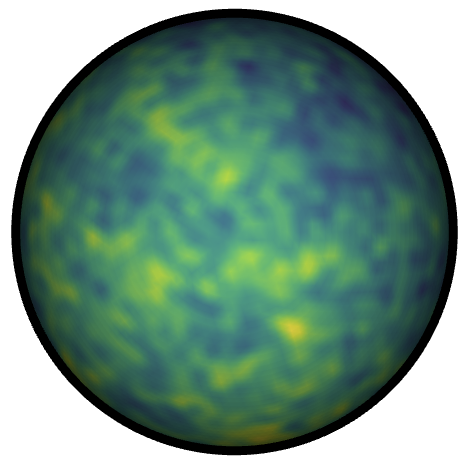
The true covariance function is approximated by truncating the infinite series in (6.5) to and the error is computed by approximating the covariance functions to be piecewise constant on an overkill mesh consisting of nodes. The resulting errors can be seen in Figure 6 together with a simulation of the field on the overkill mesh.
Based on the observed errors, linear regression is again used to compute the empirical rates of convergence for each value of . The resulting observed rates are shown in Table 3 and validate the theoretical results.

| Rates | 1.52 (1.4) | 1.76 (1.8) | 1.97 (2.0) | 2.06 (2.0) | 2.08 (2.0) |
|---|
7 Discussion
Figure 4 shows that the fully mass-lumped approximation can have a smaller error than the approximation in which mass lumping is applied only to the right-hand side. This phenomenon has previously been observed in the non-fractional case with constant . In that setting, the matrix expression for the precision operator reveals that some of the errors introduced by replacing the mass matrix with its lumped version may partially cancel when all mass matrices in the precision matrix are treated consistently.
Our results provide a theoretical justification for this observation in a much broader setting. In particular, they show that replacing the exact mass matrices by lumped ones does not reduce the convergence rate of the covariance approximation. This remains true for fractional powers of elliptic operators and for the non-stationary extensions considered in this work.
The analysis of the non-stationary variance-control factor gives an additional conclusion. For models of the form , the covariance of the solution involves multiplication by on both sides of the covariance operator associated with . In practical finite element implementations, this multiplication must also be discretized, typically through nodal interpolation or quadrature-based approximations. Our results show that the error introduced by this additional discretization is controlled by the regularity of . More precisely, if belongs to the multiplier space , which is typically of the form coupled with appropriate boundary conditions, then the covariance error contains an additional term of order . Thus, when , the discretization of the variance-control factor does not reduce the second-order convergence rate of the covariance approximation.
Thus, mass lumping is not only computationally attractive because it leads to sparse and easily invertible mass matrices, but it can also be used without sacrificing the asymptotic convergence rate of the covariance approximation, even in the fractional and non-stationary settings considered here.
References
- [1] (2026) Finite element and box-method discretizations for fractional elliptic problems with quadrature and mass lumping. Note: arXiv:2605.12082 External Links: Document, 2605.12082 Cited by: §3.2, §3.2, §4.1, §5, §5, §5.
- [2] (2014) Unified form language: a domain-specific language for weak formulations of partial differential equations. ACM Trans. Math. Software 40 (2), pp. 9:1–9:37. External Links: Document Cited by: §4.2.
- [3] (2020) Isotropic covariance functions on graphs and their edges. Ann. Statist. 48 (4), pp. 2478–2503. External Links: Document Cited by: §4.3.
- [4] (2019) Non-stationary Gaussian models with physical barriers. Spat. Stat. 29, pp. 268–288. External Links: Document Cited by: §1.1, §3.3.
- [5] (2023) DOLFINx: the next generation FEniCS problem solving environment. Zenodo. Note: DOI: 10.5281/zenodo.10447666 External Links: Document Cited by: §4.2.
- [6] (2013) Introduction to quantum graphs. Mathematical Surveys and Monographs, Vol. 186, American Mathematical Society, Providence, RI. External Links: ISBN 978-0-8218-9211-4 Cited by: §4.3.
- [7] (2018) Weak convergence of Galerkin approximations for fractional elliptic stochastic PDEs with spatial white noise. BIT Numer. Math. 58 (4), pp. 881–906. External Links: Document Cited by: §1.1.
- [8] (2020) Numerical solution of fractional elliptic stochastic PDEs with spatial white noise. IMA J. Numer. Anal. 40 (2), pp. 1051–1073. External Links: Document Cited by: §1.1.
- [9] (2020) The rational SPDE approach for Gaussian random fields with general smoothness. J. Comput. Graph. Statist. 29 (2), pp. 274–285. External Links: Document Cited by: §1.1, §1.1, Remark 3.8, §4.1.
- [10] (2023) Equivalence of measures and asymptotically optimal linear prediction for Gaussian random fields with fractional-order covariance operators. Bernoulli 29 (2), pp. 1476–1504. External Links: Document Cited by: §1.1.
- [11] (2024) Regularity and numerical approximation of fractional elliptic differential equations on compact metric graphs. Math. Comp. 93 (349), pp. 2439–2472. External Links: Document Cited by: §4.3, §4.3, §4.3, §6.2.
- [12] (2013) A comparison between Markov approximations and other methods for large spatial data sets. Comput. Statist. Data Anal. 61, pp. 7–21. External Links: Document Cited by: §1.1.
- [13] (2026) Log-Gaussian Cox process on general metric graphs. Biometrika. External Links: Document, Link Cited by: §4.3.
- [14] (2024) Gaussian Whittle–Matérn fields on metric graphs. Bernoulli 30 (2), pp. 1611–1639. External Links: Document Cited by: §4.3.
- [15] (2025) MetricGraph: random fields on metric graphs. Note: R package version 1.6.0 External Links: Link Cited by: §4.3.
- [16] (2026) Markov properties of Gaussian random fields on compact metric graphs. Bernoulli 32 (1), pp. 153–178. External Links: Document Cited by: §4.3.
- [17] (2026) Statistical inference for Gaussian Whittle–Matérn fields on metric graphs. J. R. Stat. Soc. Ser. B Stat. Methodol.. External Links: Document, Link Cited by: §4.3.
- [18] (2024) Covariance–based rational approximations of fractional SPDEs for computationally efficient Bayesian inference. J. Comput. Graph. Statist. 33 (1), pp. 64–74. External Links: Document Cited by: §3.2.1, §3.2.2, §3.2.2, Remark 3.8, §4.1, §4.1, §6.3, §6.3.
- [19] (2025) rSPDE: rational approximations of fractional stochastic partial differential equations. Note: R package version 2.5.1 External Links: Link Cited by: §4.1.
- [20] (2020) Multivariate type G Matérn stochastic partial differential equation random fields. J. R. Stat. Soc. Ser. B Stat. Methodol. 82 (1), pp. 215–239. External Links: Document Cited by: §1.1.
- [21] (2014) Spatial Matérn fields driven by non-Gaussian noise. Scand. J. Statist. 41 (3), pp. 557–579. External Links: Link, Document Cited by: §1.1.
- [22] (2024) Numerical approximation of Gaussian random fields on closed surfaces. Comput. Methods Appl. Math. 24 (4), pp. 829–858. External Links: Document Cited by: §3.2.1, §4.2.
- [23] (2019) On sinc quadrature approximations of fractional powers of regularly accretive operators. J. Numer. Math. 27 (2), pp. 57–68. External Links: Document Cited by: Remark 3.8.
- [24] (2015) Numerical approximation of fractional powers of elliptic operators. Math. Comp. 84 (295), pp. 2083–2110. External Links: Document Cited by: Remark 3.8.
- [25] (2020) Matérn Gaussian processes on Riemannian manifolds. In Advances in Neural Information Processing Systems, Vol. 33, pp. 12426–12437. Cited by: §1.1.
- [26] (2008) The mathematical theory of finite element methods. 3 edition, Texts in Applied Mathematics, Vol. 15, Springer, New York. External Links: Document Cited by: §4.1.
- [27] (2013) Spatio-temporal modeling of particulate matter concentration through the SPDE approach. AStA Adv. Stat. Anal. 97 (2), pp. 109–131. External Links: Link, Document Cited by: §1.1.
- [28] (2022) A general framework for SPDE-based stationary random fields. Bernoulli 28 (1), pp. 1–32. External Links: Document Cited by: §1.1.
- [29] (2002) The finite element method for elliptic problems. SIAM. External Links: Document Cited by: §4.1.
- [30] (2013) Measure theory: second edition. Birkhäuser Advanced Texts Basler Lehrbücher, Springer, New York. External Links: Document, ISBN 9781461469568 Cited by: §2.
- [31] (2020) Regularity and convergence analysis in Sobolev and Hölder spaces for generalized Whittle–Matérn fields. Numer. Math. 146, pp. 819–873. External Links: Document Cited by: §1.1, §1.1, §3.1, §4.1, §4.1.
- [32] (2011) Parallel distributed computing using Python. Adv. Water Resour. 34 (9), pp. 1124–1139. External Links: Document Cited by: §4.2.
- [33] (2013) Finite element methods for surface PDEs. Acta Numer. 22, pp. 289–396. External Links: Document Cited by: §4.2, §4.2, §4.2, Remark 4.5.
- [34] (1972) Effects of quadrature errors in finite element approximation of steady state, eigenvalue and parabolic problems. In The mathematical foundations of the finite element method with applications to partial differential equations, pp. 525–556. External Links: Document Cited by: §4.1.
- [35] (2015) Exploring a new class of non-stationary spatial Gaussian random fields with varying local anisotropy. Statist. Sinica 25 (1), pp. 115–133. External Links: Document Cited by: §1.1, §3.3.
- [36] (2009) Gmsh: a three-dimensional finite element mesh generator with built-in pre- and post-processing facilities. Internat. J. Numer. Methods Engrg. 79 (11), pp. 1309–1331. External Links: Document Cited by: §4.2.
- [37] (2011) Elliptic problems in nonsmooth domains. SIAM, Philadelphia. External Links: Document Cited by: §4.1.
- [38] (2024) Multilevel approximation of Gaussian random fields: covariance compression, estimation, and spatial prediction. Adv. Comput. Math. 50 (5), pp. 101. External Links: Document Cited by: §1.1.
- [39] (2020) Analysis of numerical methods for spectral fractional elliptic equations based on the best uniform rational approximation. J. Comput. Phys. 408, pp. 109285. External Links: Document Cited by: Remark 3.8.
- [40] (2020) Multilevel approximation of Gaussian random fields: fast simulation. Math. Models Methods Appl. Sci. 30 (1), pp. 181–223. External Links: Document Cited by: §1.1, §4.2.
- [41] (2021) Deformed SPDE models with an application to spatial modeling of significant wave height. Spat. Stat. 42, pp. 100449. External Links: Document Cited by: §1.1.
- [42] (2020) A unified view of some numerical methods for fractional diffusion. Comput. Math. Appl. 80 (2), pp. 332–350. External Links: Document Cited by: Remark 3.8.
- [43] (2014) Spatial models with explanatory variables in the dependence structure. Spat. Stat. 8, pp. 20–38. External Links: Document Cited by: §3.3.
- [44] (2022) Surface finite element approximation of spherical Whittle–Matérn Gaussian random fields. SIAM J. Sci. Comput. 44 (2), pp. A825–A842. External Links: Link, Document Cited by: §4.2.
- [45] (2013) Error estimates for a semidiscrete finite element method for fractional order parabolic equations. SIAM J. Numer. Anal. 51 (1), pp. 445–466. External Links: Document Cited by: §4.
- [46] (2022) Necessary and sufficient conditions for asymptotically optimal linear prediction of random fields on compact metric spaces. Ann. Statist. 50 (2), pp. 1038–1065. External Links: Document Cited by: §6.3.
- [47] (2019) Advanced spatial modeling with stochastic partial differential equations using R and INLA. Chapman and Hall/CRC, Boca Raton. External Links: Document Cited by: §3.3.
- [48] (2013) Introduction to smooth manifolds. 2 edition, Graduate Texts in Mathematics, Vol. 218, Springer, New York, NY. External Links: Document Cited by: §4.2.
- [49] (2024) A diffusion‐based spatio‐temporal extension of Gaussian Matérn fields. Stat. Oper. Res. Trans. 48 (1), pp. 3–66. External Links: Link, Document Cited by: §1.1.
- [50] (2022) The SPDE approach for Gaussian and non-Gaussian fields: 10 years and still running. Spat. Stat. 50, pp. 100599. External Links: Document Cited by: §1.1, §1.1.
- [51] (2011) An explicit link between Gaussian fields and Gaussian Markov random fields: the stochastic partial differential equation approach. J. R. Stat. Soc. Ser. B Stat. Methodol. 73 (4), pp. 423–498. External Links: Document Cited by: §1.1, §1.1, §1.1, §1.1, §4.1.
- [52] (2015) Bayesian spatial modelling with R-INLA. J. Stat. Softw. 63 (19), pp. 1–25. External Links: Document Cited by: §3.3, §4.1.
- [53] (2026) Fmesher: triangle meshes and related geometry tools. Note: R package version 0.7 External Links: Link Cited by: §4.1.
- [54] (2026) Rnaturalearth: world map data from natural earth. Note: R package version 1.2.0 External Links: Link Cited by: §4.1.
- [55] (1960) Spatial variation: Stochastic models and their application to some problems in forest surveys and other sampling investigations. Meddelanden Från Statens Skogsforskningsinstitut, Band 49, Nr. 5, Stockholm. External Links: Document Cited by: §1.1.
- [56] (1995) The Malliavin calculus and related topics. Probability and its Applications, Springer, New York. External Links: Document, ISBN 9781475724370 Cited by: §2.
- [57] (2026) OpenStreetMap data. External Links: Link Cited by: §4.3.
- [58] (2018) Simple features for R: standardized support for spatial vector data. R J. 10 (1), pp. 439–446. External Links: Document Cited by: §4.1.
- [59] (2024) The Matérn model: a journey through statistics, numerical analysis and machine learning. Statist. Sci. 39 (3), pp. 469–492. External Links: Document Cited by: §1.1.
- [60] (2026) R: a language and environment for statistical computing. R Foundation for Statistical Computing, Vienna, Austria. External Links: Link Cited by: §4.1.
- [61] (2026) Overpass turbo: a web-based data filtering tool for OpenStreetMap. External Links: Link Cited by: §4.3.
- [62] (2022) Finite element representations of Gaussian processes: balancing numerical and statistical accuracy. SIAM/ASA J. Uncertain. Quantif. 10 (4), pp. 1323–1349. External Links: Document Cited by: §1.1, §1.1.
- [63] (2022) The SPDE approach to Matérn fields: graph representations. Statist. Sci. 37 (4), pp. 519–540. External Links: Document Cited by: §1.1.
- [64] (2010) Trace ideals and their applications. Mathematical Surveys and Monographs, American Mathematical Society. External Links: Document, Link, ISBN 9781470413477 Cited by: §5.
- [65] (1993) Best uniform rational approximation of on . Bull. Amer. Math. Soc. 28 (1), pp. 116–122. External Links: Document Cited by: §3.2.2, Remark 3.8.
- [66] (2022) Cauchy Markov random field priors for Bayesian inversion. Stat. Comput. 32 (2), pp. 33. External Links: Document Cited by: §1.1.
- [67] (2007) Galerkin finite element methods for parabolic problems. Springer Series in Computational Mathematics, Vol. 25, Springer. External Links: Document Cited by: §4.1, §4.
- [68] (2015) Geostatistical modelling using non-Gaussian Matérn fields. Scand. J. Statist. 42 (3), pp. 872–890. External Links: Link, Document Cited by: §1.1.
- [69] (1963) Stochastic processes in several dimensions. Bull. Inst. Internat. Statist. 40, pp. 974–994. Cited by: §1.1.
- [70] (2012) Applied functional analysis: applications to mathematical physics. Applied Mathematical Sciences, Vol. 108, Springer. External Links: Document Cited by: §2.