Hybrid spatial–temporal graph neural network Powered NDTs: Towards Next-Gen Smart Infrastructure Twins

With inspiration from [12], we built our framework on Internet Topology Zoo, a collection of ISP network topologies transcribed into GraphML and GML [7] for use in network topology research. The dataset provides a diverse collection of real-world network topologies with varying scales and structural characteristics, enabling robust evaluation across different network conditions. It includes both medium and large-scale topologies, with node counts ranging from tens to several hundreds. This diversity supports the emulation of key 6G properties, particularly heterogeneous network integration and network-of-networks architectural concept [21]. As summarized in Table I, a combined graph of 1210 nodes and 1572 initial edges was used in our framework, augmented to 4354 edges after preprocessing for GNN input. All features where normalized to $[0,1]$ with min-max scaling for improved model performance [22]. The dataset split followed a train/validation/test split as additionally shown in Table I, preventing label leakages.

The 10-dimensional feature vector $\mathbf{x}_{i}$ for node $i$ included: degree, betweenness centrality, clustering coefficient, closeness centrality, PageRank, latitude, longitude, 2-hop neighborhood degree, eigenvector centrality, and core number. These features are of optimal importance and adopted in graph-based learning to capture both structural importance and spatial context [23, 17]. Table II summarizes the statistical properties of the raw node features prior to min-max normalization.

The target features (RTT & packet loss) adopted in our study were generated through a topology-driven simulation procedure. In the implementation, edge attributes such as geographic distance, propagation delay, link capacity, and utilization were derived from the connected network graph. Traffic demand was then emulated between sampled source-destination pairs using weighted shortest paths, allowing the underlying model to reflect topology-aware routing behavior in a controlled and reproducible setting. For each node, RTT was modeled as a function of path-level propagation delay, queueing delay driven by utilization, and additive noise, which is consistent with work showing that queueing delay dominates total network delay and that latency-based feedback can resolve very fine-grained queuing effects [16]. Packet loss was generated from a congestion-sensitive probability model, which fits the literature showing that packet loss can be bursty at sub-RTT timescales and tightly coupled to queueing behavior [28]. This design framework preserves reproducibility while producing targets that are closer to real network behavior.

Rather than choosing a single GNN paradigm, HSTGNN adopts a hybrid spatio-temporal design that fuses static and dynamic graphs and uses a GRU with graph convolution to model temporal evolution and spatial dependencies [30], while combining three complementary message-passing mechanisms in parallel. This hybrid structure matches recent spatial-temporal graph models that aggregate neighbors within each slice of a graph, exchange information across graph slices over time, and combine graph Fourier or spectral convolution operators with attention-based or temporal gated modules. These representations are then refined in stacked layers or blocks, which is consistent with architectures that repeat hierarchical aggregation or block-wise temporal modeling across depth. Additionally, this hybrid design framework follows recent trends demonstrating that combining spatial, spectral, and attention-based GNNs improves representational power and generalization [13].

$\mathbf{H}^{(\ell)}$ denoting the hidden representation at layer $\ell$. Each multi-scale block contains three parallel branches:

Branch 1 – Local (GraphSAGE):

$$\mathbf{h}_{i}^{(\text{sage})}=\sigma\left(\mathbf{W}_{1}\left[\mathbf{h}_{i}^{(\ell)}\,\|\,\mathrm{AGG}_{j\in\mathcal{N}(i)}\mathbf{h}_{j}^{(\ell)}\right]\right),$$

(1)

which captures local neighborhood structures through inductive aggregation.

Branch 2 – Spectral (Chebyshev):

$$\mathbf{h}_{i}^{(\text{cheb})}=\sum_{k=0}^{K}\theta_{k}T_{k}(\tilde{\mathbf{L}})\mathbf{h}_{i}^{(\ell)},$$

(2)

Branch 3 – Attention (TransformerConv):

$$\mathbf{h}_{i}^{(\text{attn})}=\sum_{j\in\mathcal{N}(i)\cup\{i\}}\alpha_{ij}\mathbf{W}_{3}\mathbf{h}_{j}^{(\ell)},$$

(3)

where $\tilde{\mathbf{L}}=\mathbf{I}_{N}-\mathbf{D}^{-1/2}\mathbf{A}\mathbf{D}^{-1/2}$ is the normalized graph Laplacian and $K=3$ in the proposed model and $\alpha_{ij}$ are learned attention coefficients that adaptively quantify the relative importance of each neighbor.

The branch outputs are concatenated and passed through a learned channel-gating mechanism:

$$\mathbf{h}_{i}^{(\text{cat})}=\left[\mathbf{h}_{i}^{(\text{sage})}\,\|\,\mathbf{h}_{i}^{(\text{cheb})}\,\|\,\mathbf{h}_{i}^{(\text{attn})}\right],$$

(4)

$$\mathbf{h}_{i}^{(\ell+1)}=\phi\left(\mathbf{g}^{(\ell)}\odot\mathbf{h}_{i}^{(\text{cat})}+\mathbf{R}\mathbf{h}_{i}^{(\ell)}\right),$$

(5)

where $\mathbf{g}^{(\ell)}$ is a learned channel gate, $\mathbf{R}$ is a residual projection, and $\phi(\cdot)$ denotes normalization and nonlinearity.

The full HSTGNN architecture stacked three such multi-scale blocks. After these blocks, two learnable temporal modulation modules apply channel-wise scale-shift transformations and feed-forward refinement. A final multi-head graph attention layer further refines the learned representation. The output stage combines graph-derived and raw-feature-derived representations through a learned mixing mechanism and adds a direct skip connection from the input features to the prediction head. This design improves expressiveness while maintaining stable optimization.

Training followed a full-graph node-regression setting using the AdamW optimizer, learning-rate scheduling, gradient clipping, and early stopping. The training objective combined Huber loss, mean squared error, and a ramped correlation-based term:

$$\mathcal{L}_{\text{HSTGNN}}=0.50\,\mathcal{L}_{\text{Huber}}+0.25\,\mathcal{L}_{\text{MSE}}+0.25\,r(t)\,\mathcal{L}_{\text{corr}},$$

(6)

where $r(t)$ is a ramp factor that gradually increases the influence of the correlation term during training.

For the baseline models, the training objective is:

$$\mathcal{L}_{\text{base}}=\mathcal{L}_{\text{MSE}}+0.05\,\mathcal{L}_{\text{L1}}.$$

(7)

For efficient evaluation, the models were trained and their final performance evaluated on a held-out test set using $R^{2}$, MAE, RMSE, and Huber loss as key evaluation metrics. The coefficient of determination $R^{2}$ defined as:

$$R^{2}=1-\frac{\sum_{i=1}^{n}(y_{i}-\hat{y}_{i})^{2}}{\sum_{i=1}^{n}(y_{i}-\bar{y})^{2}}$$

(8)

capturing the proportion of variance explained by the model and providing a measure of overall goodness-of-fit [5]. Mean Absolute Error computed as:

$$\text{MAE}=\frac{1}{n}\sum_{i=1}^{n}|y_{i}-\hat{y}_{i}|$$

(9)

reflecting the average magnitude of prediction errors and offering an interpretable measure of typical deviation [4]. Root Mean Squared Error given by:

$$\text{RMSE}=\sqrt{\frac{1}{n}\sum_{i=1}^{n}(y_{i}-\hat{y}_{i})^{2}}$$

(10)

penalizing larger errors more strongly due to its quadratic nature [4]. Finally, Huber loss which combines squared-error and absolute-error behavior [14]:

$$L_{\delta}(y,\hat{y})=\frac{1}{n}\sum_{i=1}^{n}\begin{cases}\frac{1}{2}(y_{i}-\hat{y}_{i})^{2}&\text{if }|y_{i}-\hat{y}_{i}|\leq\delta\\ \delta\left(|y_{i}-\hat{y}_{i}|-\frac{\delta}{2}\right)&\text{otherwise}\end{cases}$$

(11)

making it less sensitive to outliers (with $\delta=0.1$ in our experimentation framework).

In this subsection and the following ones, we provide an analysis of the results obtained. As demonstrated in Figures 3 and  4, HSTGNN achieved the highest coefficient of determination with $R^{2}\approx 0.8816$, while also obtaining the lowest MAE $\approx 0.0300$, the lowest RMSE $\approx 0.0458$, and the lowest Huber loss $\approx 0.00093$. These results show that the proposed hybrid model produces the most accurate and most stable predictions overall. Among the baseline methods, ChebNet is the strongest with $R^{2}\approx 0.7504$, MAE $\approx 0.0477$, and RMSE $\approx 0.0703$, followed closely by GraphSAGE with $R^{2}\approx 0.7503$, ResGatedGCN with $R^{2}\approx 0.7478$, and GraphTransformer with $R^{2}\approx 0.7363$.

The fact that HSTGNN outperforms the rest in all error performance metrics indicates that the framework is not only accurate on average, but is also less prone to large prediction errors. This makes the framework more aligned for practical NDT deployment, where occasional large estimation errors can be operationally costly especially in replicating the physical network (PT).

Additionally, the prediction-versus-actual scatter plots in Figure. 5 provide additional qualitative evidence of HSTGNN’s superiority. For a well-calibrated model, predictions should cluster closely around the diagonal identity line. In the scatter plots, HSTGNN exhibits the tightest concentration around this line compared to the highest performing baseline ChebNet. This visual pattern is significant because it confirms that the performance gain is not merely numerical but also visual, showing that HSTGNN produces predictions that track the true RTT values more closely across the full output range.

Moreover, Table III highlights the practical gain of HSTGNN over the strongest baseline. In absolute terms, the model improves $R^{2}$ by $17.5\%$. In relative terms, it reduces MAE by $37.1\%$ and RMSE by $34.9\%$, while also requiring substantially fewer epochs $\approx 146$ to converge. This is an important result because it shows that the performance advantage of HSTGNN is not achieved at the expense of optimization stability. Instead, the framework is both more accurate and more resource efficient during training.

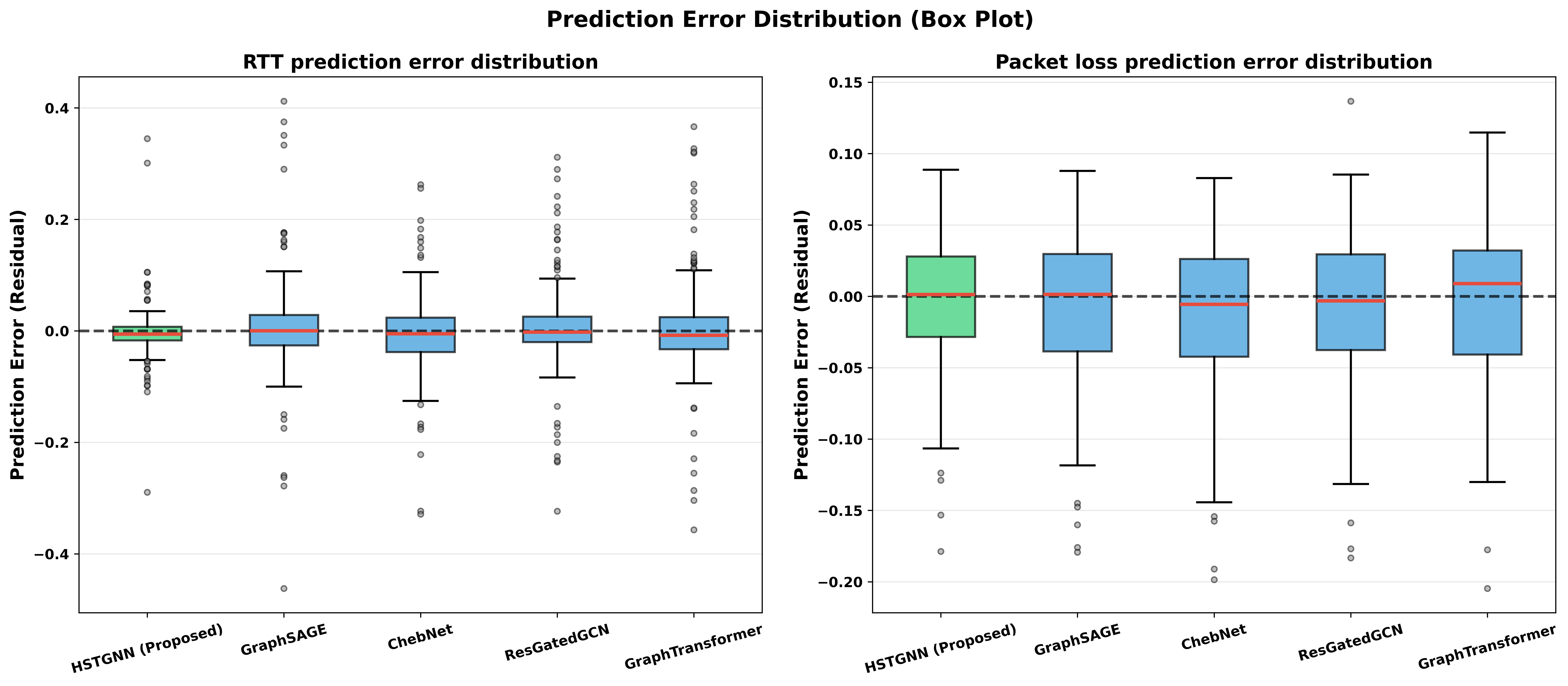
As the authors in [15] suggest, low variance in prediction errors is a critical requirement for reliable Network Digital Twin deployment, because it reflects the consistency and stability of model outputs under inherently stochastic network conditions In AI driven frameworks, high variability in errors is closely associated with increased uncertainty and reduced trustworthiness of predictions, even when average accuracy appears competitive [10]. Therefore, minimizing error variance is essential for ensuring reproducible and dependable model behavior in real-world environments. The presented plots in Figure 6 clearly demonstrates that HSTGNN achieves substantially lower error variance than all baseline model frameworks, as evidenced by the tightly concentrated distributions around zero for both RTT and packet loss predictions. Such compact distributions indicate highly consistent predictions across varying conditions, which is essential for operational decision-making in dynamic networks.

A NDT is expected to provide reliable predictions of operational metrics before control actions are applied to the real system in a closed loop framework [3]. In the results obtained, the proposed model achieves strong performance on both RTT and packet loss jointly, which is significant because these two metrics reflect complementary aspects of service quality that is, latency and reliability. The results also suggest that HSTGNN is suitable for scenarios involving planning, validation, and what-if case analysis. The lower MAE and RMSE imply more trustworthy prediction outputs, while the higher $R^{2}$ indicates that the framework captures the main patterns governing network behavior. Together, these properties strengthen the usefulness of the proposed architecture as a predictive framework inside a mobile network digital twin. Moreover, in Table IV we show experimental findings in a broader systems context where we show alignment of these capabilities with the direction of 6G intelligent networking and with 3GPP standadization road-map related to analytics-driven automation, service assurance, and closed-loop control. The experimental evidence indicates that the proposed architecture is well positioned for such future integration.

References

- [1] (2026) Release 18 and 19: 5g-advanced. Note: https://www.3gpp.org/specifications-technologies/releasesAccessed 2026 Cited by: TABLE IV.
- [2] (2024) Artificial intelligence in 6g wireless networks: opportunities, applications, and challenges. International Journal of Intelligent Systems 2024 (1), pp. 8845070. External Links: Document, Link Cited by: TABLE IV.
- [3] (2023) Digital twins for next-generation mobile networks: applications and solutions. IEEE Communications Magazine 61 (11), pp. 80–86. Cited by: §V-C, TABLE IV.
- [4] (2014) Root mean square error (rmse) or mean absolute error (mae)? – arguments against avoiding rmse in the literature. Geoscientific Model Development. External Links: Document Cited by: §IV-C, §IV-C.
- [5] (2021) The coefficient of determination r-squared is more informative than smape, mae, mape, mse and rmse in regression analysis evaluation. Peerj computer science 7, pp. e623. Cited by: §IV-C.
- [6] (2026) The promise of 6g. In 6G-life, pp. 3–16. Cited by: §I, TABLE IV.
- [7] (2026) 3D Internet Zoo: A 3D visualization of the Internet topology Zoo with Google Earth. Note: https://github.com/afourmy/3D-internet-zooGitHub repository, accessed 2026 Cited by: Figure 1, §I, §III-A.
- [8] (2011) Packet loss and delay measurement for mpls networks. RFC 6374, pp. 1–52. External Links: Link Cited by: §I.
- [9] (2008) Managing complex network operation with predictive analytics. In AAAI Spring Symposium: Technosocial Predictive Analytics, External Links: Link Cited by: §I.
- [10] (2021) Aleatoric and epistemic uncertainty in machine learning: an introduction to concepts and methods. Machine learning 110 (3), pp. 457–506. Cited by: §V-B.
- [11] (2022-01) Digital-twin-enabled 6g: vision, architectural trends, and future directions. IEEE Communications Magazine 60 (1), pp. 74–80. External Links: Document Cited by: TABLE IV.
- [12] (2011) The internet topology zoo. IEEE Journal on Selected Areas in Communications 29 (9), pp. 1765–1775. External Links: Document Cited by: §III-A.
- [13] (2022) Survey of graph neural networks and applications. Wireless Communications and Mobile Computing. External Links: Document Cited by: §IV-A.
- [14] (2021) An alternative probabilistic interpretation of the huber loss. In Proceedings of the ieee/cvf conference on computer vision and pattern recognition, pp. 5261–5269. Cited by: §IV-C.
- [15] (2025) Towards a robust transport network with self-adaptive network digital twin. Computer Networks, pp. 111967. Cited by: §V-B.
- [16] (2015) Latency-based congestion detection and control for datacenters major advisor :. External Links: Link Cited by: §III-C.
- [17] (2023) Empowering digital twin for future networks with graph neural networks: overview, enabling technologies, challenges, and opportunities. Future Internet 15 (12), pp. 377. External Links: Document Cited by: §II, §III-B.
- [18] (2025) Network digital twin toward networking, telecommunications, and traffic engineering: a survey. IEEE Access 13 (), pp. 16489–16538. External Links: Document Cited by: §I.
- [19] (2020) RouteNet: leveraging graph neural networks for network modeling and optimization in sdn. IEEE Journal on Selected Areas in Communications 38 (10), pp. 2260–2270. External Links: Document Cited by: §I, §II.
- [20] (2023) 5G-enabled internet of things: latency optimization through ai-assisted network slicing. pp. 1–10. External Links: Document Cited by: §I.
- [21] (2025) MultiNet6G: 5g nr, wifi and visible light communication working as single network. In 2025 IEEE Conference on Standards for Communications and Networking (CSCN), Vol. , pp. 1–7. External Links: Document Cited by: §III-A.
- [22] (2023) A novel approach for data feature weighting using correlation coefficients and min–max normalization. Symmetry 15, pp. 2185. External Links: Document Cited by: §III-A.
- [23] (2022) Graph neural networks for intelligent modelling in network management and orchestration: a survey on communications. Electronics 11 (20). External Links: Document Cited by: §II, §III-B.
- [24] (2020) Challenges towards automation of live telco network management: closed control loops. In 2020 16th International Conference on Network and Service Management (CNSM), Vol. , pp. 1–5. External Links: Document Cited by: §I.
- [25] (2022) A graph neural network-based digital twin for network slicing management. IEEE Transactions on Industrial Informatics 18 (2), pp. 1367–1376. External Links: Document Cited by: §II.
- [26] (2025) Hybrid spatio-temporal graph neural network with attention fusion for traffic flow prediction. Knowledge-Based Systems 324, pp. 113813. Cited by: §II.
- [27] (2025) Hybrid spatial–temporal graph neural network for traffic forecasting. Information Fusion 118, pp. 102978. Cited by: §II.
- [28] (2007) Packet loss burstiness: measurements and implications for distributed applications. In 2007 IEEE International Parallel and Distributed Processing Symposium, pp. 1–8. Cited by: §III-C.
- [29] (2025) On effectiveness of graph neural network architectures for network digital twins (ndts). pp. 1–6. Cited by: §I, §II.
- [30] (2025) A review of hyperspectral image classification based on graph neural networks. Artificial Intelligence Review 58. External Links: Document Cited by: §IV-A.
- [31] (2020) Graph neural networks: a review of methods and applications. AI open 1, pp. 57–81. Cited by: §I.