Bayesian Distilled Clustering for High-Dimensional Mixture Models

Pulkita Aggarwal Corresponding author: pulkitaaggarwal09@gmail.com pulkitaaggarwal09@gmail.com Abhishek Bhattacharjee Corresponding author: abhishek@theabstractmath.com abhishek@theabstractmath.com

1 Introduction

Latent subgroup analysis is a central problem in modern statistics, with applications in genomics, precision medicine, social science, and large-scale observational studies. In these settings, the observed population is often heterogeneous, and the scientific objective is not merely to predict an outcome, but to identify interpretable subpopulations with distinct covariate structure, response behavior, or dependence patterns. Mixture models provide a natural probabilistic framework for this task. They allow the data-generating distribution to be represented as a weighted combination of subgroup-specific laws, with the subgroup label treated as an unobserved random variable.

The high-dimensional regime presents a more delicate problem. When the number of measured covariates is large, only a small subset of variables may be responsible for meaningful subgroup separation. The remaining variables may contain measurement noise, nuisance variation, or correlation induced by the relevant covariates, but they need not carry independent information about subgroup membership. Standard clustering methods often treat all variables as exchangeable inputs. In high dimensions, this can be statistically inefficient and scientifically misleading: irrelevant coordinates accumulate noise, distort distances, and may obscure the low-dimensional structure that defines the latent classes.

This paper develops a Bayesian distilled clustering framework for high-dimensional mixture models. The basic premise is that clustering should be carried out in a statistically justified subspace rather than in the full ambient space. The proposed method first uses a Bayesian variable-selection model to estimate posterior inclusion probabilities for the covariates. These probabilities quantify the evidence that each covariate contributes to subgroup separation or subgroup-specific response behavior. A distilled covariate set is then obtained by controlling the posterior expected false-discovery proportion. Clustering is subsequently performed only on this selected subspace. Finally, within each inferred subgroup, conditional-independence diagnostics are used to study subgroup-specific dependence among the selected variables.

The formulation is deliberately model-based. The selected variables are not obtained by marginal screening, nor by a generic dimension-reduction criterion. Instead, the distillation step is tied to the mixture structure and to the response model. This makes the resulting subspace directly aligned with the scientific object of interest: latent subgroups that differ in distributional structure and response behavior.

1.1 Existing Works

The literature on variable selection for clustering problems from a frequentist perspective includes methods based on the ideas of sparse K-means by Witten and Tibshirani (2010), pairwise penalized model-based clustering by Guo et al. (2010), and L1-penalized EM algorithms for finite mixtures of regressions by Städler et al. (2010). The extension of the latter approach to group-lasso penalization without sample splitting was provided by Wang et al. (2024). None of these methods maintain an uncertainty measure over the selected set of variables and do not provide a means of controlling the false discoveries of variables within the selection step.

The Bayesian approach to variable selection in clustering was first considered by Tadesse et al. (2005). Kim et al. (2006) extended this approach to Dirichlet process mixtures. Raftery and Dean (2006) employed a likelihood approach to model variable selection, where models including and excluding each variable were compared using Bayes factors and greedy search procedures. Maugis et al. (2009) considered variable selection within Dirichlet process mixtures, but with a more careful modeling of the dependence between relevant and irrelevant variables. In each of these approaches, however, no asymptotic theoretical results are provided for cases in which the number of variables p is allowed to grow at a much faster rate than the number of observations n, and where a response model is included that is specific to subgroups of the clustering algorithm results.

The posterior concentration theory for high-dimensional Bayesian variable selection was developed by Castillo and van der Vaart (2012), and also by Castillo et al. (2015). The theory applies to the type of spike-and-slab priors with complexity penalties that have been used in this paper. Scott and Berger (2010) provided an analysis of the multiplicity properties of these priors. The posterior false-discovery rate rule is based upon the approaches of Newton et al. (2004) and Müller et al. (2004).

The graphical diagnostics for the subgroups is based upon the graphical lasso method of Friedman et al. (2008) and the debiasing approach of Janková and van de Geer (2015), who prove that the debiased graphical lasso estimator is asymptotically normal entry-wise. Thus, statistical tests can be performed on each graphical edge within the estimated subgroups. A false-discovery rate control rule for graphical edges is that of Benjamini and Hochberg (1995).

The approach of this paper unifies these methods in a way that does not appear in the existing literature. While the variable selection and clustering steps are separate in terms of their computational approach, the two methods are based upon the same underlying probabilistic model that encompasses both the subgroup-specific covariate distribution and the response variable. Furthermore, the choice of subspace is based upon the posterior false-discovery rate rule rather than upon model selection methods. Asymptotic guarantees are established for each of the steps of the approach: variable selection, information preservation, clustering, response variable estimation, and graphical model estimation.

1.2 Our contributions

The main contributions are as follows.

•

We introduce a Bayesian distillation framework for high-dimensional mixture models in which feature selection and clustering are separated computationally but connected through a common probabilistic model.
•

We define posterior inclusion probabilities for covariates and use them to construct a distilled covariate set with posterior false-discovery control. This provides a principled alternative to marginal screening or unsupervised dimension reduction.
•

We show that, under a conditional-irrelevance assumption, the excluded covariates contain no additional subgroup information once the distilled variables are known. Consequently, the Bayes classifier based on all covariates coincides with the Bayes classifier based only on the relevant covariates.
•

We establish theoretical properties of the procedure, including posterior selection consistency, preservation of subgroup information after distillation, clustering consistency, posterior contraction for subgroup-specific response parameters, and validity of subgroup-level conditional-independence tests.
•

We formulate a subgroup-specific graphical diagnostic based on conditional independence. In the Gaussian case, this diagnostic is expressed through the precision matrix within each inferred subgroup and allows the analyst to study how selected covariates interact differently across latent classes.
•

We provide a simulation framework for evaluating variable-selection accuracy, cluster recovery, prediction, and graph recovery in high-dimensional mixture settings.

1.3 Structure of the paper

The remainder of the paper is organized as follows. Section 2 gives the statistical model and defines the relevant covariate set. Section 3 presents the Bayesian distillation model, including the prior specification, posterior inclusion probabilities, and posterior false-discovery rule. Section 4 describes the clustering step on the distilled subspace. Section 5 introduces subgroup-specific conditional-independence diagnostics. Section 6 states the assumptions and theoretical guarantees. Section 7 summarizes the practical implementation. Section 8 gives a recommended simulation design. Section 9 concludes. Proofs are collected in Appendix A.

2 Statistical Setting

Let

D_{n}=\{(Y_{i},X_{i}):1\leq i\leq n\}

be independent observations, where $Y_{i}\in\mathcal{Y}$ is a response and

X_{i}=(X_{i1},\ldots,X_{ip})^{\top}\in\mathbb{R}^{p}

is a high-dimensional covariate vector. The dimension $p$ may be much larger than $n$ . The population is assumed to contain $K$ latent subgroups. For each subject $i$ , let

Z_{i}\in\{1,\ldots,K\}

denote the unobserved subgroup label, with

\mathbb{P}(Z_{i}=k)=\pi_{k},\qquad\pi_{k}>0,\qquad\sum_{k=1}^{K}\pi_{k}=1.

The central statistical assumption is that only a small subset of covariates carries information about the latent subgroup structure and the subgroup-specific response behavior. Let

S_{0}\subset\{1,\ldots,p\}

be the unknown set of relevant covariates, with

|S_{0}|=s_{0}\ll p.

The complement $S_{0}^{c}$ consists of variables that may be noisy, correlated, or biologically measurable, but do not help distinguish the latent subgroups after the variables in $S_{0}$ are known.

For a candidate subset $S$ , write $X_{iS}$ for the coordinates of $X_{i}$ indexed by $S$ . A rigorous model for the joint distribution of $(Y_{i},X_{i})$ is

p(y,x)=\sum_{k=1}^{K}\pi_{k}q_{k}(x_{S};\psi_{k})r_{k}(y\mid x_{S};\theta_{k})h(x_{S^{c}}\mid x_{S}),

where $q_{k}$ is the subgroup-specific covariate density on the selected coordinates, $r_{k}$ is the subgroup-specific response model, and $h$ is the conditional distribution of the excluded variables. The key structural restriction is that $h$ does not depend on $k$ . Thus the excluded variables may be statistically dependent on the selected variables, but they do not contain additional subgroup information once $X_{S}$ is known.

A concrete Gaussian version, useful for theory and implementation, is

X_{iS_{0}}\mid Z_{i}=k\sim N_{s_{0}}(\mu_{k0},\Sigma_{k0}),

and

Y_{i}\mid X_{i},Z_{i}=k\sim f\{y;\eta_{ik},\phi_{k}\},\qquad\eta_{ik}=\alpha_{k}+X_{iS_{0}}^{\top}\beta_{k0}.

Here $f$ may be a Gaussian, Bernoulli, Poisson, or other regular exponential-family density. The covariates outside $S_{0}$ satisfy

p(X_{iS_{0}^{c}}\mid X_{iS_{0}},Z_{i}=k)=p(X_{iS_{0}^{c}}\mid X_{iS_{0}})

for every $k$ . Therefore, irrelevant variables may still be statistically associated with relevant variables, but they do not help separate the latent groups.

This distinction is important. A variable is not called irrelevant merely because it has small marginal variance or weak marginal association with the response. It is irrelevant only if it contributes neither to subgroup separation nor to subgroup-specific response behavior after the selected variables are accounted for.

3 Bayesian Distillation Model

Introduce a binary inclusion vector

\gamma=(\gamma_{1},\ldots,\gamma_{p})^{\top}\in\{0,1\}^{p},

where

\gamma_{j}=\begin{cases}1,&\text{if covariate }j\text{ is included},\\ 0,&\text{otherwise}.\end{cases}

Let

S_{\gamma}=\{j:\gamma_{j}=1\}.

For a given $\gamma$ , define the observed-data likelihood

L_{n}(\Theta,\gamma)=\prod_{i=1}^{n}\sum_{k=1}^{K}\pi_{k}q_{k}(X_{iS_{\gamma}};\psi_{k})r_{k}(Y_{i}\mid X_{iS_{\gamma}};\theta_{k}),

where

\Theta=\{\pi_{k},\psi_{k},\theta_{k}:1\leq k\leq K\}.

The variables outside $S_{\gamma}$ are not used in the clustering likelihood because, under the model, their conditional distribution does not depend on the latent subgroup once $X_{iS_{\gamma}}$ is given.

A sparse prior is placed on $\gamma$ . One convenient choice is the complexity prior

\mathbb{P}(\gamma)\propto c^{-|\gamma|}p^{-a|\gamma|},\qquad a>1,\ c>0,

where

|\gamma|=\sum_{j=1}^{p}\gamma_{j}.

This prior penalizes large models strongly enough to prevent the posterior from including many irrelevant variables when $p$ is large.

Conditional on $\gamma$ , the mixture weights have prior

(\pi_{1},\ldots,\pi_{K})\sim\operatorname{Dirichlet}(a_{\pi},\ldots,a_{\pi}),

and the subgroup-specific parameters receive proper continuous priors. For example, in the Gaussian covariate model,

\mu_{k,S_{\gamma}}\mid\Sigma_{k,S_{\gamma}}\sim N_{|S_{\gamma}|}(m_{0},\kappa_{0}^{-1}\Sigma_{k,S_{\gamma}}),

and

\Sigma_{k,S_{\gamma}}^{-1}\sim\operatorname{Wishart}(\nu_{0},A_{0}).

For the response model,

\beta_{k,S_{\gamma}}\sim N_{|S_{\gamma}|}(0,\tau_{\beta}^{2}I),\qquad\alpha_{k}\sim N(0,\tau_{\alpha}^{2}).

The posterior distribution is

\Pi(\Theta,\gamma\mid D_{n})=\frac{L_{n}(\Theta,\gamma)p(\Theta\mid\gamma)p(\gamma)}{\sum_{\gamma^{\prime}}\int L_{n}(\Theta^{\prime},\gamma^{\prime})p(\Theta^{\prime}\mid\gamma^{\prime})p(\gamma^{\prime})\,d\Theta^{\prime}}.

For each variable $j$ , define its posterior inclusion probability

w_{j}=\Pi(\gamma_{j}=1\mid D_{n}).

The distilled set is chosen by controlling the posterior expected false-discovery proportion. For a threshold $t\in[0,1]$ , define

\widehat{S}(t)=\{j:w_{j}\geq t\}.

The posterior expected false-discovery proportion is

\operatorname{BFDR}(t)=\frac{\sum_{j:w_{j}\geq t}(1-w_{j})}{|\widehat{S}(t)|\vee 1}.

For a preassigned level $q\in(0,1)$ , choose

\widehat{t}=\inf\{t:\operatorname{BFDR}(t)\leq q\},

and set

\widehat{S}=\widehat{S}(\widehat{t}).

This rule has a clear interpretation: among the selected variables, the posterior expected fraction of irrelevant variables is at most $q$ .

4 Clustering on the Distilled Subspace

After the distilled set $\widehat{S}$ is obtained, the clustering step is performed only on $X_{i\widehat{S}}$ . The primary clustering model is

X_{i\widehat{S}}\mid Z_{i}=k\sim q_{k}(\cdot;\psi_{k}),\qquad\mathbb{P}(Z_{i}=k)=\pi_{k}.

In the Gaussian version,

X_{i\widehat{S}}\mid Z_{i}=k\sim N_{|\widehat{S}|}(\mu_{k,\widehat{S}},\Sigma_{k,\widehat{S}}).

Let

\widehat{\Psi}=\{\widehat{\pi}_{k},\widehat{\mu}_{k},\widehat{\Sigma}_{k}:1\leq k\leq K\}

denote the fitted mixture parameters. The posterior membership weight for observation $i$ and subgroup $k$ is

\widehat{r}_{ik}=\frac{\widehat{\pi}_{k}\varphi_{|\widehat{S}|}(X_{i\widehat{S}};\widehat{\mu}_{k},\widehat{\Sigma}_{k})}{\sum_{\ell=1}^{K}\widehat{\pi}_{\ell}\varphi_{|\widehat{S}|}(X_{i\widehat{S}};\widehat{\mu}_{\ell},\widehat{\Sigma}_{\ell})}.

The estimated subgroup label is

\widehat{Z}_{i}=\operatorname*{arg\,max}_{1\leq k\leq K}\widehat{r}_{ik}.

The response $Y_{i}$ may be incorporated in two ways. In the primary version, $Y_{i}$ is used to guide variable selection, but cluster assignment is based on the covariate subspace. This respects the goal of identifying covariate-defined latent subgroups. In a supervised extension, one may assign labels by the joint posterior weight

\widehat{r}_{ik}^{\mathrm{joint}}=\frac{\widehat{\pi}_{k}q_{k}(X_{i\widehat{S}};\widehat{\psi}_{k})r_{k}(Y_{i}\mid X_{i\widehat{S}};\widehat{\theta}_{k})}{\sum_{\ell=1}^{K}\widehat{\pi}_{\ell}q_{\ell}(X_{i\widehat{S}};\widehat{\psi}_{\ell})r_{\ell}(Y_{i}\mid X_{i\widehat{S}};\widehat{\theta}_{\ell})}.

The covariate-only version is preferred when the scientific target is subgroup discovery. The joint version is useful when the target is response-stratified prediction.

5 Conditional-Independence Diagnostics Within Subgroups

For each estimated subgroup $k$ , define

\widehat{\mathcal{I}}_{k}=\{i:\widehat{Z}_{i}=k\},\qquad\widehat{n}_{k}=|\widehat{\mathcal{I}}_{k}|.

The goal is to study how the selected variables depend on one another within each subgroup. In the Gaussian case,

X_{i\widehat{S}}\mid Z_{i}=k\sim N(\mu_{k},\Sigma_{k}),

and the conditional-independence structure is encoded by the precision matrix

\Omega_{k}=\Sigma_{k}^{-1}.

For two distinct selected variables $a,b\in\widehat{S}$ ,

X_{a}\perp X_{b}\mid X_{\widehat{S}\setminus\{a,b\}},Z=k\quad\Longleftrightarrow\quad(\Omega_{k})_{ab}=0.

Thus the subgroup-specific graph is

G_{k}=(\widehat{S},E_{k}),

where

(a,b)\in E_{k}\quad\Longleftrightarrow\quad(\Omega_{k})_{ab}\neq 0.

A high-dimensional estimator of $\Omega_{k}$ may be obtained using a penalized likelihood,

\widehat{\Omega}_{k}=\operatorname*{arg\,min}_{\Omega\succ 0}\left\{\operatorname{tr}(\widehat{\Sigma}_{k}\Omega)-\log\det(\Omega)+\lambda_{k}\sum_{a\neq b}|\Omega_{ab}|\right\},

where $\widehat{\Sigma}_{k}$ is the sample covariance matrix within subgroup $k$ .

For inference on individual edges, use a debiased estimator $\widehat{\Omega}_{k,ab}^{d}$ . The test statistic is

T_{k,ab}=\frac{\sqrt{\widehat{n}_{k}}\widehat{\Omega}_{k,ab}^{d}}{\widehat{\sigma}_{k,ab}}.

Under the null hypothesis

H_{0,k,ab}:(\Omega_{k})_{ab}=0,

the statistic satisfies

T_{k,ab}\rightsquigarrow N(0,1).

The resulting $p$ -values are adjusted within each subgroup using the Benjamini-Hochberg procedure. This yields a subgroup-specific dependence graph with controlled false discoveries.

6 Theoretical Properties

The following results are stated for a clean Gaussian version of the model. This is the natural first theory for the proposed method. Extensions to generalized responses or non-Gaussian covariates require the same structure: identifiability, sparsity, regular priors, and concentration of likelihood ratios.

6.1 Assumptions

Assumption 6.1 (Sparse truth).

There exists a true subset $S_{0}\subset\{1,\ldots,p\}$ with

|S_{0}|=s_{0},\qquad s_{0}\log p=o(n).

The true inclusion vector is $\gamma_{0}$ , where $(\gamma_{0})_{j}=1$ if and only if $j\in S_{0}$ .

This condition formalizes the high-dimensional regime in which only a small number of covariates drive the mixture structure and the subgroup-specific response model. The requirement $s_{0}\log p=o(n)$ is the usual effective-sample-size condition for recovering a sparse subset among $p$ candidates. It links the distillation step to the central statistical goal of the paper: clustering should be performed on the variables that carry subgroup information, not on the full ambient feature space.

Assumption 6.2 (Irrelevant variables contain no subgroup information).

For all $k$ ,

p_{0}(X_{S_{0}^{c}}\mid X_{S_{0}},Z=k)=p_{0}(X_{S_{0}^{c}}\mid X_{S_{0}}).

Thus $X_{S_{0}^{c}}$ may be correlated with $X_{S_{0}}$ , but it carries no additional information about $Z$ .

This assumption gives a precise meaning to irrelevance in the mixture setting. Variables in $S_{0}^{c}$ are allowed to be correlated with the selected variables, so the condition does not impose marginal independence. Rather, it requires that, after conditioning on $X_{S_{0}}$ , the remaining variables do not further distinguish the latent subgroups. This is the population-level justification for distillation: removing $S_{0}^{c}$ should reduce noise without removing information about the latent class.

Assumption 6.3 (Identifiability).

For $k\neq\ell$ ,

(\mu_{k0},\Sigma_{k0},\alpha_{k},\beta_{k0},\phi_{k})\neq(\mu_{\ell 0},\Sigma_{\ell 0},\alpha_{\ell},\beta_{\ell 0},\phi_{\ell}).

The mixture is identifiable up to relabeling of the $K$ components.

The latent classes must correspond to distinct data-generating mechanisms. Since mixture labels are inherently arbitrary, identifiability is required only up to permutation of the component labels. Without this condition, neither posterior concentration nor clustering consistency has a well-defined target. The assumption ensures that the inferred subgroups can be compared to a population-level mixture decomposition rather than to an artifact of parameterization.

Assumption 6.4 (Eigenvalue control).

There exist constants $0<c<C<\infty$ such that, for every $k$ ,

c\leq\lambda_{\min}(\Sigma_{k0})\leq\lambda_{\max}(\Sigma_{k0})\leq C.

This condition rules out degenerate or nearly singular within-component covariance matrices. It prevents subgroup separation from being created by ill-conditioned covariance structure rather than by stable distributional differences. The bounded-eigenvalue condition is also needed for likelihood concentration, Gaussian tail bounds, and precision-matrix inference within subgroups.

Assumption 6.5 (Signal strength).

For every $j\in S_{0}$ , the variable has detectable subgroup or response signal. Define

b_{j}=\max_{k\neq\ell}|\mu_{kj,0}-\mu_{\ell j,0}|+\max_{k}|\beta_{kj,0}|.

Assume

\min_{j\in S_{0}}b_{j}\geq b_{n},

where

nb_{n}^{2}\geq C_{1}\log p

for a sufficiently large constant $C_{1}$ .

Each relevant variable must leave a detectable trace either through subgroup separation or through the subgroup-specific response model. The lower bound $nb_{n}^{2}\geq C_{1}\log p$ is a beta-min condition adapted to the high-dimensional setting. It separates true variables from noise at the scale needed to search over many candidate covariates. This condition is what makes posterior distillation possible rather than merely descriptive.

Assumption 6.6 (Component separation).

Define

\Delta_{n}=\min_{k\neq\ell}\left[(\mu_{k0}-\mu_{\ell 0})^{\top}\Sigma_{0}^{-1}(\mu_{k0}-\mu_{\ell 0})\right]^{1/2},

where $\Sigma_{0}$ is a representative within-component covariance, such as a common covariance in the homoscedastic case. Assume

\Delta_{n}\to\infty

for vanishing clustering error, and

\Delta_{n}^{2}\geq C_{2}\log n

for exact recovery with probability tending to one.

The quantity $\Delta_{n}$ measures the minimum separation between latent components in the informative subspace. Consistent clustering cannot be expected when components overlap too strongly, even if the correct variables are known. The stronger logarithmic separation condition gives exact label recovery with high probability. This assumption connects the variable-selection part of the method to the downstream clustering target: after the relevant subspace has been recovered, the components must still be statistically distinguishable.

Assumption 6.7 (Prior regularity).

The prior on $\gamma$ satisfies

\mathbb{P}(\gamma)\propto c^{-|\gamma|}p^{-a|\gamma|},\qquad a>1,

and the parameter priors have continuous densities that are positive in neighborhoods of the true parameter values.

The prior assigns enough mass near the true sparse model while penalizing unnecessarily large models. The factor $p^{-a|\gamma|}$ , with $a>1$ , prevents the posterior from favoring large models that improve the likelihood only by fitting noise. Positivity of the parameter priors near the truth ensures that the Bayesian procedure does not exclude the data-generating parameter values. Together, these conditions make posterior model selection compatible with high-dimensional sparsity.

6.2 Posterior Selection Consistency

Theorem 6.1 (Posterior selection consistency).

Under Assumptions 6.1, 6.3, 6.5, and 6.7,

\Pi(\gamma=\gamma_{0}\mid D_{n})\longrightarrow 1

in $P_{0}$ -probability. Consequently,

\max_{j\in S_{0}}(1-w_{j})\to 0,\qquad\max_{j\notin S_{0}}w_{j}\to 0

in $P_{0}$ -probability. Therefore, for any fixed threshold $t\in(0,1)$ ,

\widehat{S}(t)=S_{0}

with probability tending to one.

The posterior inclusion probabilities separate relevant and irrelevant variables asymptotically. Relevant variables receive inclusion probability tending to one, while irrelevant variables receive inclusion probability tending to zero. This gives the distillation step a formal target: the selected subspace converges to the population subspace that drives subgroup and response heterogeneity.

The proof is given in Appendix A.1.

6.3 Information Preservation After Distillation

Theorem 6.2 (Information preservation after distillation).

Under Assumption 6.2, the Bayes classifier based on all variables $X$ is identical to the Bayes classifier based only on $X_{S_{0}}$ . That is,

\operatorname*{arg\,max}_{k}\mathbb{P}(Z=k\mid X)=\operatorname*{arg\,max}_{k}\mathbb{P}(Z=k\mid X_{S_{0}}).

The relevant subspace is sufficient for optimal subgroup classification. Discarding $X_{S_{0}^{c}}$ does not change the population Bayes rule because those variables contain no additional class information once $X_{S_{0}}$ is known. This property is central to the paper’s construction: distillation is not merely a computational reduction, but a statistically lossless reduction for the clustering target under the stated model.

The proof is given in Appendix A.2.

6.4 Clustering Consistency

Theorem 6.3 (Clustering consistency).

Assume Theorem 6.1 holds and Assumptions 6.2, 6.4, and 6.6 hold. Let $\widehat{Z}_{i}$ be the label obtained by fitting the mixture model on $X_{i\widehat{S}}$ . Then, up to a permutation of component labels,

\frac{1}{n}\sum_{i=1}^{n}\mathbf{1}(\widehat{Z}_{i}\neq Z_{i})=O_{P}\{\exp(-c\Delta_{n}^{2})\}+o_{P}(1)

for some constant $c>0$ .

If, in addition,

\Delta_{n}^{2}\geq C\log n

for a sufficiently large constant $C$ , then

\mathbb{P}\left(\min_{\sigma\in\mathfrak{S}_{K}}\max_{1\leq i\leq n}\mathbf{1}\{\widehat{Z}_{i}\neq\sigma(Z_{i})\}=0\right)\to 1,

where $\mathfrak{S}_{K}$ is the set of all permutations of $\{1,\ldots,K\}$ .

Once the distilled subspace recovers the relevant variables, clustering in that subspace attains the usual Gaussian-mixture classification behavior. The error rate is governed by the separation $\Delta_{n}$ , not by the ambient dimension $p$ . This supports the two-stage design: posterior distillation controls the high-dimensional feature problem, while mixture clustering then operates in the statistically relevant coordinates.

The proof is given in Appendix A.3.

6.5 Posterior Contraction for the Response Model

Theorem 6.4 (Posterior contraction for the response model).

Suppose the response model is a regular exponential-family regression model and Assumptions 6.1, 6.3, 6.5, and 6.7 hold. Then, after relabeling the mixture components,

\Pi\left(\max_{1\leq k\leq K}\|\beta_{k,S_{0}}-\beta_{k0,S_{0}}\|_{2}>M\sqrt{\frac{s_{0}\log p}{n}}\ \middle|\ D_{n}\right)\to 0

in $P_{0}$ -probability for a sufficiently large constant $M$ . The same rate holds for $\mu_{k,S_{0}}$ under the Gaussian covariate model.

After model selection, the subgroup-specific response parameters concentrate at the standard sparse high-dimensional rate. The rate depends on $s_{0}\log p$ , rather than on the full dimension $p$ . This result links clustering to inference: the distilled variables are not only useful for label recovery, but also support stable estimation of subgroup-specific response relationships.

The proof is given in Appendix A.4.

6.6 Validity of Subgroup Conditional-Independence Tests

Theorem 6.5 (Validity of subgroup conditional-independence tests).

Assume the subgroup-specific covariate distribution is Gaussian. For subgroup $k$ , let

\Omega_{k0}=\Sigma_{k0}^{-1}.

Assume $\Omega_{k0}$ is sparse, with maximum node degree $d_{k}$ , and

d_{k}^{2}\frac{\log s_{0}}{n_{k}}\to 0,

where

n_{k}=\#\{i:Z_{i}=k\}.

Assume also that Theorem 6.3 gives exact recovery of the subgroup labels with probability tending to one.

Then, for every null edge $(a,b)$ satisfying

(\Omega_{k0})_{ab}=0,

the debiased statistic satisfies

T_{k,ab}\rightsquigarrow N(0,1).

Consequently, if the Benjamini-Hochberg procedure is applied within subgroup $k$ , the false-discovery rate satisfies

\operatorname{FDR}_{k}\leq q+o(1).

Moreover, if for a nonzero edge

\frac{\sqrt{n_{k}}|(\Omega_{k0})_{ab}|}{\sigma_{k,ab}}\to\infty,

then the probability of detecting that edge tends to one.

The subgroup-specific graphical analysis remains valid after clustering, provided the labels are recovered with high probability and the precision matrices are sufficiently sparse. The result separates two sources of uncertainty: label uncertainty is controlled by the clustering theorem, and edge-level uncertainty is handled by debiased precision-matrix inference. This gives a formal basis for using the inferred subgroups to study conditional dependence structures among the distilled variables.

The proof is given in Appendix A.5.

7 Practical Methodology

7.1 Step 1: Preprocessing

Each covariate is centered and scaled. For biological data, variables with extreme missingness or near-zero variance are removed before modeling. Missing values may be handled by model-based imputation, but the imputation model should be fit inside the training folds when cross-validation is used.

7.2 Step 2: Bayesian Variable Distillation

Fit the Bayesian mixture-response model with sparse inclusion vector $\gamma$ . Compute posterior inclusion probabilities

w_{j}=\Pi(\gamma_{j}=1\mid D_{n}).

Select

\widehat{S}=\{j:w_{j}\geq\widehat{t}\}

using posterior false-discovery control.

This step is not a marginal screening rule. A variable is selected because the posterior evidence supports its role in subgroup separation, subgroup-specific response behavior, or both.

7.3 Step 3: Refit the Mixture on the Distilled Subspace

Fit a finite mixture model to

\{X_{i\widehat{S}}:1\leq i\leq n\}.

Compute posterior membership weights $\widehat{r}_{ik}$ and assign

\widehat{Z}_{i}=\operatorname*{arg\,max}_{k}\widehat{r}_{ik}.

Uncertainty should be reported through the entropy

H_{i}=-\sum_{k=1}^{K}\widehat{r}_{ik}\log\widehat{r}_{ik}.

Subjects with large $H_{i}$ are weakly assigned and should not be overinterpreted.

7.4 Step 4: Estimate Subgroup-Specific Response Models

Within each inferred subgroup, fit

Y_{i}\mid X_{i\widehat{S}},\widehat{Z}_{i}=k.

This provides subgroup-specific associations between the selected covariates and the response. These estimates are useful for interpretation, prediction, and treatment-effect heterogeneity analysis.

7.5 Step 5: Conditional-Independence Diagnostics

For each subgroup $k$ , estimate the precision matrix $\Omega_{k}$ of $X_{\widehat{S}}$ . Test

H_{0,k,ab}:(\Omega_{k})_{ab}=0

for all pairs $a\neq b$ . Adjust the resulting $p$ -values using Benjamini-Hochberg within each subgroup.

The output is a collection of graphs

\widehat{G}_{1},\ldots,\widehat{G}_{K},

where each graph describes conditional dependence among selected variables inside one subgroup.

7.6 Step 6: Model Checking

The following checks should be reported:

1.

Stability of $\widehat{S}$ under resampling.
2.

Stability of cluster assignments under resampling.
3.

Posterior uncertainty of $K$ , if $K$ is not fixed.
4.

Predictive performance for $Y$ .
5.

Separation of clusters in the selected subspace.
6.

Sensitivity to the posterior false-discovery level $q$ .
7.

Sensitivity to the prior on model size.

8 Simulation Studies

A rigorous simulation study should vary the following factors:

n\in\{100,300,500\},\qquad p\in\{500,2000,10000\},

and

s_{0}\in\{5,10,25\},\qquad K\in\{2,3,5\}.

Generate latent labels

Z_{i}\sim\operatorname{Categorical}(\pi_{1},\ldots,\pi_{K}).

For $j\in S_{0}$ , generate subgroup-dependent covariates. For $j\notin S_{0}$ , generate noise covariates that may be correlated with $S_{0}$ , but do not depend on $Z_{i}$ after conditioning on $X_{iS_{0}}$ .

Generate responses from

Y_{i}=\alpha_{Z_{i}}+X_{iS_{0}}^{\top}\beta_{Z_{i}}+\varepsilon_{i},\qquad\varepsilon_{i}\sim N(0,\sigma^{2}),

or from a logistic model for binary outcomes.

Report:

\text{variable-selection TPR},\qquad\text{variable-selection FDR},\qquad\text{adjusted Rand index},

and

\text{misclassification rate},\qquad\text{prediction error},\qquad\text{graph edge FDR},\qquad\text{graph edge power}.

The main comparisons should include full-dimensional Gaussian mixtures, sparse $K$ -means, penalized mixture models, spectral clustering on all variables, and clustering after marginal screening.

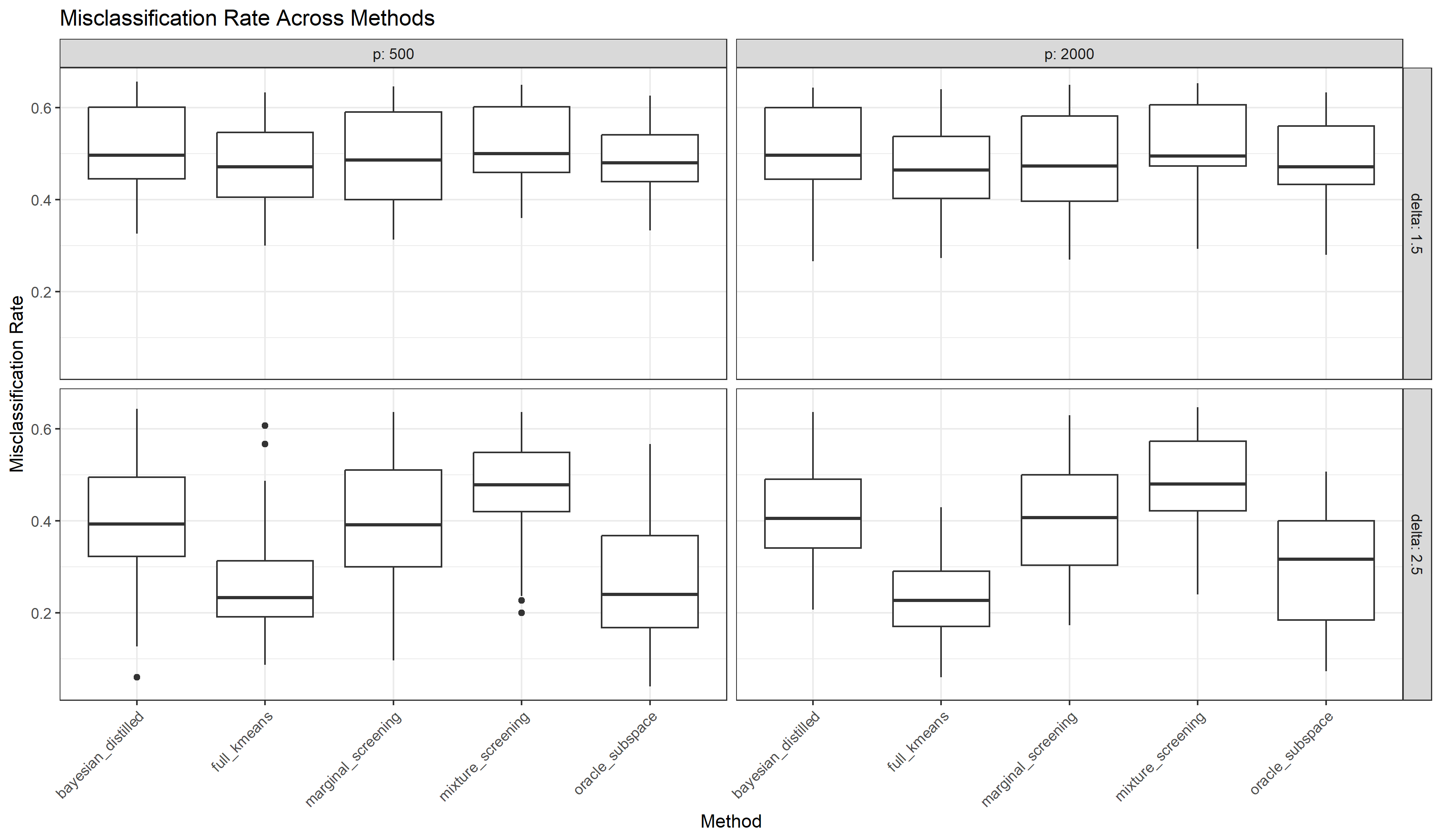
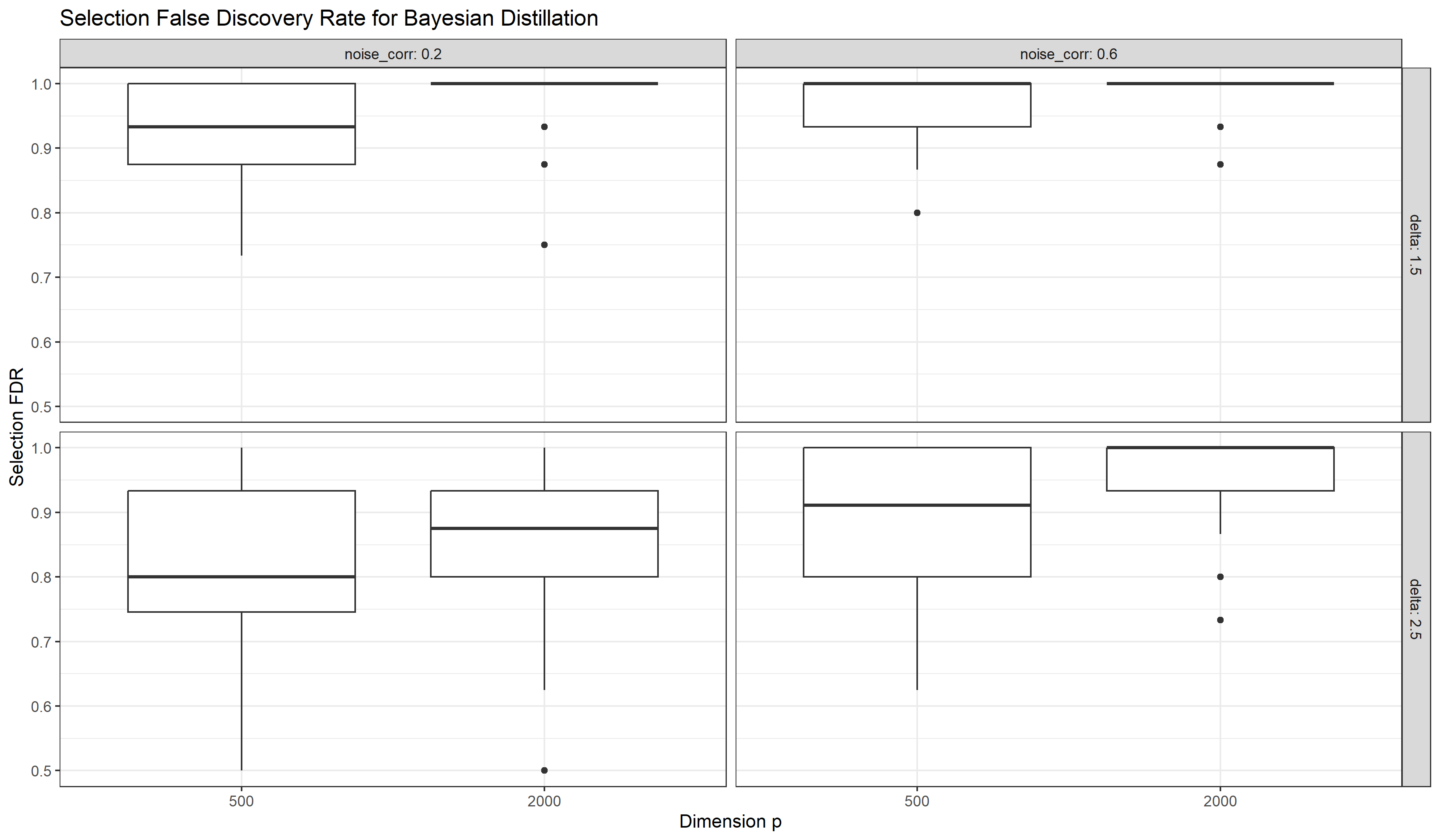
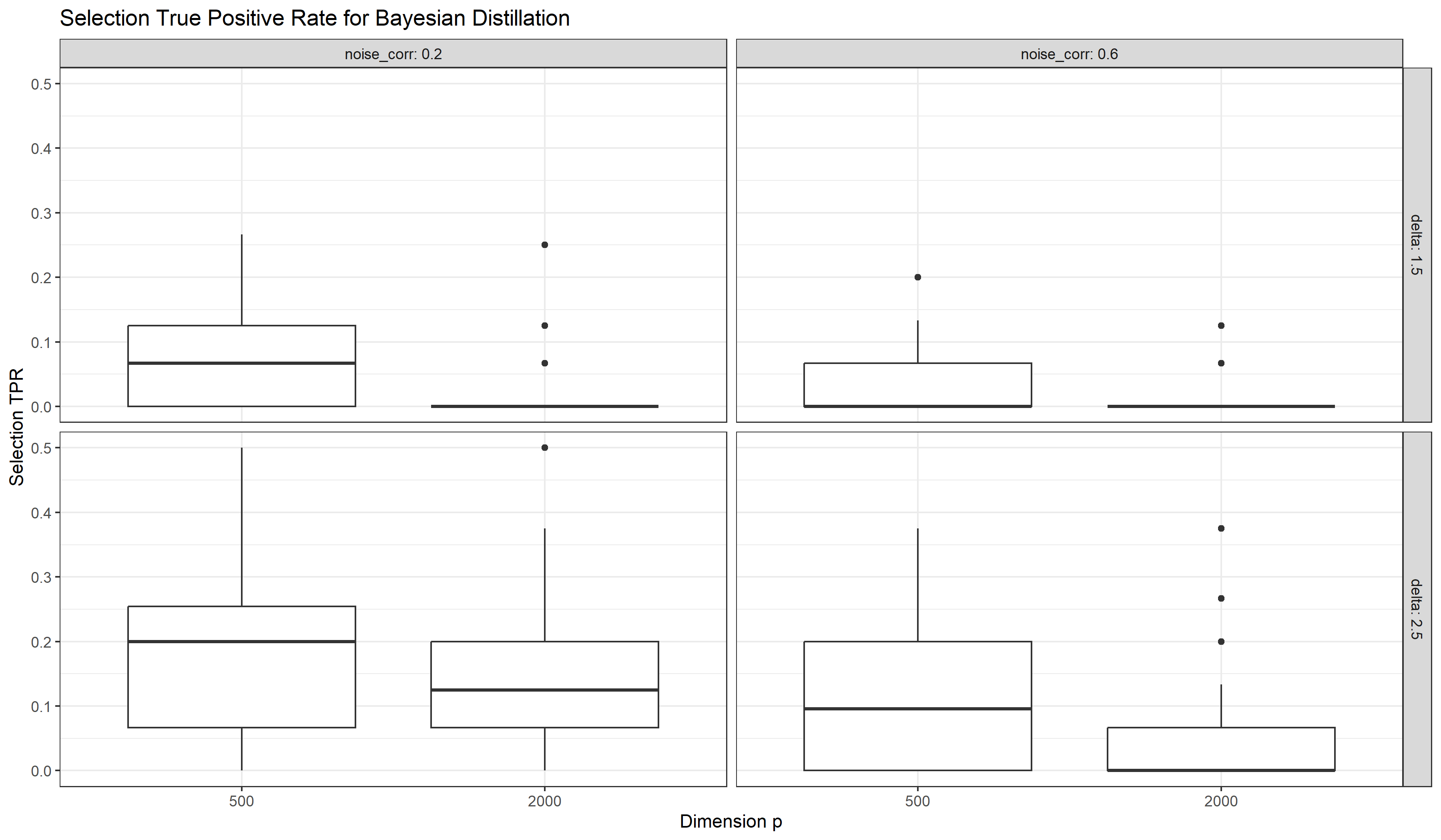
The central empirical claim should be modest and testable: when the relevant subgroup information is sparse, Bayesian distillation should reduce noise accumulation and improve both variable recovery and cluster recovery relative to methods that treat all variables equally.

For the details, we refer to the following diagrams.

Refer to caption — Figure 1: Adjusted rank index across methods

9 Conclusion

High-dimensional clustering is most useful when the recovered groups correspond to interpretable and reproducible sources of heterogeneity. In mixture models, this objective is difficult to achieve when the relevant subgroup information is sparse and embedded in a large number of nuisance variables. The framework developed here addresses this difficulty by placing variable selection before clustering, while preserving a coherent probabilistic link between the selected variables, the latent subgroup labels, and the response.

The proposed procedure has three features that are especially important in scientific applications. First, the distilled subspace is selected using posterior evidence, rather than by marginal association or purely geometric dimension reduction. Second, clustering is performed only after the high-dimensional noise has been attenuated, which improves both interpretability and statistical stability. Third, the subgroup-specific conditional-independence analysis provides a second layer of inference: after the subgroups are estimated, one may examine how the selected variables relate to one another within each subgroup.

The theory formalizes these points. Under sparsity, signal-strength, identifiability, and separation conditions, the posterior concentrates on the true relevant variables, the distilled subspace preserves subgroup information, and the clustering rule consistently recovers the latent labels. Under additional sparsity assumptions on subgroup-specific precision matrices, conditional-independence tests within the estimated subgroups are asymptotically valid. These results support the use of Bayesian distillation as a principled tool for high-dimensional subgroup discovery, particularly in settings such as genomics and multi-omics studies where interpretability, uncertainty quantification, and structural insight are all central to the analysis.

References

Y. Benjamini and Y. Hochberg (1995) Controlling the false discovery rate: a practical and powerful approach to multiple testing. Journal of the Royal Statistical Society: Series B (Methodological) 57 (1), pp. 289–300. External Links: Document Cited by: §1.1.
I. Castillo, J. Schmidt-Hieber, and A. van der Vaart (2015) Bayesian linear regression with sparse priors. The Annals of Statistics 43 (5), pp. 1986–2018. External Links: Document Cited by: §1.1.
I. Castillo and A. van der Vaart (2012) Needles and straw in a haystack: posterior concentration for possibly sparse sequences. The Annals of Statistics 40 (4), pp. 2069–2101. External Links: Document Cited by: §1.1.
J. Friedman, T. Hastie, and R. Tibshirani (2008) Sparse inverse covariance estimation with the graphical lasso. Biostatistics 9 (3), pp. 432–441. External Links: Document Cited by: §1.1.
J. Guo, E. Levina, G. Michailidis, and J. Zhu (2010) Pairwise variable selection for high-dimensional model-based clustering. Biometrics 66 (3), pp. 793–804. External Links: Document Cited by: §1.1.
J. Janková and S. van de Geer (2015) Confidence intervals for high-dimensional inverse covariance estimation. Electronic Journal of Statistics 9 (1), pp. 1205–1229. External Links: Document Cited by: §1.1.
S. Kim, M. G. Tadesse, and M. Vannucci (2006) Variable selection in clustering via Dirichlet process mixture models. Biometrika 93 (4), pp. 877–893. External Links: Document Cited by: §1.1.
C. Maugis, G. Celeux, and M. Martin-Magniette (2009) Variable selection for clustering with Gaussian mixture models. Biometrics 65 (3), pp. 701–709. External Links: Document Cited by: §1.1.
P. Müller, G. Parmigiani, C. Robert, and J. Rousseau (2004) Optimal sample size for multiple testing: the case of gene expression microarrays. Journal of the American Statistical Association 99 (468), pp. 990–1001. External Links: Document Cited by: §1.1.
M. A. Newton, A. Noueiry, D. Sarkar, and P. Ahlquist (2004) Detecting differential gene expression with a semiparametric hierarchical mixture method. Biostatistics 5 (2), pp. 155–176. External Links: Document Cited by: §1.1.
A. E. Raftery and N. Dean (2006) Variable selection for model-based clustering. Journal of the American Statistical Association 101 (473), pp. 168–178. External Links: Document Cited by: §1.1.
J. G. Scott and J. O. Berger (2010) Bayes and empirical-Bayes multiplicity adjustment in the variable-selection problem. The Annals of Statistics 38 (5), pp. 2587–2619. External Links: Document Cited by: §1.1.
N. Städler, P. Bühlmann, and S. van de Geer (2010) $\ell_{1}$ -Penalization for mixture regression models. TEST 19 (2), pp. 209–256. Note: With discussion External Links: Document Cited by: §1.1.
M. G. Tadesse, N. Sha, and M. Vannucci (2005) Bayesian variable selection in clustering high-dimensional data. Journal of the American Statistical Association 100 (470), pp. 602–617. External Links: Document Cited by: §1.1.
N. Wang, X. Zhang, and Q. Mai (2024) Statistical analysis for a penalized EM algorithm in high-dimensional mixture linear regression model. Journal of Machine Learning Research 25 (222), pp. 1–85. Cited by: §1.1.
D. M. Witten and R. Tibshirani (2010) A framework for feature selection in clustering. Journal of the American Statistical Association 105 (490), pp. 713–726. External Links: Document Cited by: §1.1.

Appendix A Appendix A - Proofs of Results

A.1 Proof of Theorem 6.1

Proof of Theorem 6.1.

Write the posterior probability of an incorrect model as

\Pi(\gamma\neq\gamma_{0}\mid D_{n})=\frac{\sum_{\gamma\neq\gamma_{0}}m_{\gamma}(D_{n})p(\gamma)}{\sum_{\gamma^{\prime}}m_{\gamma^{\prime}}(D_{n})p(\gamma^{\prime})},

where

m_{\gamma}(D_{n})=\int L_{n}(\Theta,\gamma)p(\Theta\mid\gamma)\,d\Theta

is the marginal likelihood under model $\gamma$ .

It is enough to show that

\sum_{\gamma\neq\gamma_{0}}\frac{m_{\gamma}(D_{n})p(\gamma)}{m_{\gamma_{0}}(D_{n})p(\gamma_{0})}\to 0.

Separate the incorrect models into two classes.

First, consider underfitted models, for which $S_{\gamma}\not\supset S_{0}$ . Such a model excludes at least one truly relevant variable. By Assumption 6.5, excluding that variable causes a loss in Kullback-Leibler risk of at least order $b_{n}^{2}$ . Therefore there exists $c_{0}>0$ such that

\inf_{\Theta}\operatorname{KL}(p_{0},p_{\Theta,\gamma})\geq c_{0}b_{n}^{2},

where $\operatorname{KL}(p_{0},p_{\Theta,\gamma})$ is the Kullback-Leibler divergence from the true density to the best density under model $\gamma$ . Standard likelihood concentration gives

\frac{m_{\gamma}(D_{n})}{m_{\gamma_{0}}(D_{n})}\leq\exp\{-c_{1}nb_{n}^{2}\}

with $P_{0}$ -probability tending to one. Since $nb_{n}^{2}\geq C_{1}\log p$ , and $C_{1}$ is sufficiently large, the sum of these ratios over all underfitted models tends to zero.

Second, consider overfitted models, for which $S_{\gamma}\supsetneq S_{0}$ . These models contain the true variables and at least one irrelevant variable. Their likelihood can improve only by fitting noise. The marginal likelihood automatically penalizes the additional dimension. More precisely, for a model with

m=|S_{\gamma}|-s_{0}

extra variables,

\frac{m_{\gamma}(D_{n})}{m_{\gamma_{0}}(D_{n})}=O_{P_{0}}(n^{-c_{2}m})

for some $c_{2}>0$ . The prior contributes the additional factor

\frac{p(\gamma)}{p(\gamma_{0})}=c^{-m}p^{-am}.

The number of models with $m$ extra variables is at most $\binom{p}{m}\leq p^{m}$ . Hence

\sum_{m\geq 1}p^{m}p^{-am}n^{-c_{2}m}=\sum_{m\geq 1}p^{-(a-1)m}n^{-c_{2}m}\to 0

because $a>1$ . Thus the total posterior mass on overfitted models vanishes.

Combining the two cases yields

\Pi(\gamma\neq\gamma_{0}\mid D_{n})\to 0,

which proves the result. ∎

A.2 Proof of Theorem 6.2

Proof of Theorem 6.2.

By Bayes’ rule,

\mathbb{P}(Z=k\mid X)=\frac{\pi_{k}p(X\mid Z=k)}{\sum_{\ell=1}^{K}\pi_{\ell}p(X\mid Z=\ell)}.

Write $X=(X_{S_{0}},X_{S_{0}^{c}})$ . Then

p(X\mid Z=k)=p(X_{S_{0}}\mid Z=k)p(X_{S_{0}^{c}}\mid X_{S_{0}},Z=k).

By Assumption 6.2,

p(X_{S_{0}^{c}}\mid X_{S_{0}},Z=k)=p(X_{S_{0}^{c}}\mid X_{S_{0}})

for all $k$ . Therefore,

\mathbb{P}(Z=k\mid X)=\frac{\pi_{k}p(X_{S_{0}}\mid Z=k)p(X_{S_{0}^{c}}\mid X_{S_{0}})}{\sum_{\ell=1}^{K}\pi_{\ell}p(X_{S_{0}}\mid Z=\ell)p(X_{S_{0}^{c}}\mid X_{S_{0}})}.

The common factor $p(X_{S_{0}^{c}}\mid X_{S_{0}})$ cancels, so

\mathbb{P}(Z=k\mid X)=\frac{\pi_{k}p(X_{S_{0}}\mid Z=k)}{\sum_{\ell=1}^{K}\pi_{\ell}p(X_{S_{0}}\mid Z=\ell)}=\mathbb{P}(Z=k\mid X_{S_{0}}).

Thus the selected subspace preserves all subgroup information. ∎

A.3 Proof of Theorem 6.3

Proof of Theorem 6.3.

Let

A_{n}=\{\widehat{S}=S_{0}\}.

By Theorem 6.1,

\mathbb{P}(A_{n})\to 1.

On $A_{n}$ , clustering is performed on exactly the true informative variables. By Theorem 6.2, no subgroup information is lost by ignoring $S_{0}^{c}$ .

For Gaussian mixtures with bounded eigenvalues and identifiable components, the fitted mixture parameters are consistent up to label switching. Thus

\max_{k}\left(\|\widehat{\mu}_{k}-\mu_{k0}\|+\|\widehat{\Sigma}_{k}-\Sigma_{k0}\|+|\widehat{\pi}_{k}-\pi_{k0}|\right)=o_{P}(1)

after a suitable relabeling.

The misclassification rate of the plug-in classifier is therefore asymptotically equal to that of the Bayes classifier. For two Gaussian components with Mahalanobis distance $\Delta_{n}$ , standard Gaussian tail bounds imply that the probability of assigning an observation from one component to the other is at most

C_{0}\exp(-c_{0}\Delta_{n}^{2})

for constants $C_{0},c_{0}>0$ . Taking the union over the finite number of component pairs gives

\mathbb{P}(\widehat{Z}_{i}\neq Z_{i})\leq C_{1}\exp(-c_{1}\Delta_{n}^{2})+o(1).

Averaging over $i$ gives

\frac{1}{n}\sum_{i=1}^{n}\mathbf{1}(\widehat{Z}_{i}\neq Z_{i})=O_{P}\{\exp(-c_{1}\Delta_{n}^{2})\}+o_{P}(1).

If $\Delta_{n}^{2}\geq C\log n$ , then

n\exp(-c_{1}\Delta_{n}^{2})\to 0

for sufficiently large $C$ . Hence, by the union bound,

\mathbb{P}(\exists i:\widehat{Z}_{i}\neq Z_{i})\to 0,

again up to label permutation. This proves exact recovery. ∎

A.4 Proof of Theorem 6.4

Proof of Theorem 6.4.

By Theorem 6.1, the posterior places probability tending to one on the true model $S_{0}$ . It is therefore sufficient to prove the contraction rate conditional on $S_{0}$ .

Within the true model, the effective parameter dimension is of order $Ks_{0}$ . The log likelihood is locally quadratic around the true parameter, and the Fisher information matrix has eigenvalues bounded away from zero and infinity under the regularity assumptions. Hence, for parameters at Euclidean distance $r_{n}$ from the truth,

r_{n}=M\sqrt{\frac{s_{0}\log p}{n}},

the likelihood ratio is bounded by

\exp(-cnr_{n}^{2})=\exp(-cM^{2}s_{0}\log p)

outside the ball of radius $r_{n}$ .

The prior assigns at least

\exp(-Cs_{0}\log p)

mass to a neighborhood of the true parameter. Choosing $M$ sufficiently large makes the likelihood decay outside the ball dominate the prior mass denominator. Standard testing arguments for parametric models with growing dimension then give

\Pi(\|\beta-\beta_{0}\|_{2}>Mr_{n}\mid D_{n},S_{0})\to 0.

Combining this with $\Pi(S_{0}\mid D_{n})\to 1$ proves the result. ∎

A.5 Proof of Theorem 6.5

Proof of Theorem 6.5.

By Theorem 6.3, with probability tending to one the estimated subgroup labels equal the true subgroup labels up to permutation. Conditional on this event, the sample used for subgroup $k$ is an independent sample from

N(\mu_{k0},\Sigma_{k0}).

Under the sparsity condition

d_{k}^{2}\frac{\log s_{0}}{n_{k}}\to 0,

the graphical-lasso or nodewise-regression estimator has elementwise error small enough for debiasing. The debiased estimator admits the expansion

\sqrt{n_{k}}\left(\widehat{\Omega}_{k,ab}^{d}-\Omega_{k0,ab}\right)=\frac{1}{\sqrt{n_{k}}}\sum_{i:Z_{i}=k}\xi_{i,ab}+o_{P}(1),

where $\xi_{i,ab}$ are mean-zero random variables with variance $\sigma_{k,ab}^{2}$ . The central limit theorem gives

\frac{\sqrt{n_{k}}(\widehat{\Omega}_{k,ab}^{d}-\Omega_{k0,ab})}{\widehat{\sigma}_{k,ab}}\rightsquigarrow N(0,1).

Under the null $\Omega_{k0,ab}=0$ , this is exactly the stated result for $T_{k,ab}$ . The Benjamini-Hochberg false-discovery control follows because the null $p$ -values are asymptotically uniform. The additional error caused by estimated labels is $o(1)$ , since exact recovery holds with probability tending to one.

For a nonzero edge, the statistic has mean

\frac{\sqrt{n_{k}}\Omega_{k0,ab}}{\sigma_{k,ab}},

which diverges by assumption. Therefore the rejection probability tends to one. ∎