GeV $\gamma$-ray emission in the star-forming region S140

In the subsequent analyses, we adopt the following fitting strategy: we allow the normalizations of all sources within a radius of $5^{\circ}$ from the ROI center (including the normalizations of the Galactic diffuse emission and the isotropic background components) to vary, and we also thaw all spectral parameters of sources within a radius of $1^{\circ}$ from the ROI center. All these free parameters are then fitted simultaneously. For clarity of presentation, we show a square region of $2^{\circ}\times 2^{\circ}$ centered on the ROI. The nearest $\gamma$-ray source to the ROI center (i.e., the MYSO S140 IRS1) is 4FGL J2220.8+6319, with Galactic coordinates $(l=106.95^{\circ},b=5.22^{\circ})$. Its angular separation from S140 IRS1 is $0.18^{\circ}$.

Within this $2^{\circ}\times 2^{\circ}$ region, we focus on three $\gamma$-ray sources, whose spatial positions are shown in Fig. 1. We first perform a fit in the $0.1$–$500~\mathrm{GeV}$ energy band. The fitting results are as follows:

• •

  4FGL J2220.8+6319: This is our target source, with $\mathrm{TS}=651.5$, $N_{\mathrm{pred}}=11909.5$, and a Log-Parabola(LP) spectrum:

  $$\frac{dN}{dE}=N_{0}\left(\frac{E}{E_{b}}\right)^{-\alpha-\beta\ln(E/E_{b})}.$$

  (1)

  The spectral parameters are $\alpha=2.85$, $\beta=0.40$, $E_{b}=1385\,\mathrm{MeV}$;

• •

  4FGL J2221.6+6349c: $\mathrm{TS}=83.5$, $N_{\mathrm{pred}}=2601.0$, also with a LP spectrum, with parameters $\alpha=2.38$, $\beta=0.39$, $E_{b}=1396\,\mathrm{MeV}$;

• •

  4FGL J2217.5+6346: $\mathrm{TS}=212.7$, $N_{\mathrm{pred}}=370.0$, also a LP spectrum, with $\alpha=1.51$, $\beta=0.42$, $E_{b}=5269\,\mathrm{MeV}$. In addition, this source is marked as being associated with the X-ray source 1RXS J221728.9+634714 (Voges et al., 2000).

Next, we selected events with energies above 1 GeV and re-localized the above three sources using the localize method in Fermipy. The positional offsets for 4FGL J2220.8+6319 and 4FGL J2217.5+6346 are $0.01^{\circ}$ and $0.02^{\circ}$, respectively, while that for 4FGL J2221.6+6349c is $0.13^{\circ}$. This relatively large offset can be understood from Fig. 1, as its TS distribution appears diffuse. In the subsequent analysis, we retain the original positions of all three sources. On the other hand, by analyzing the above information, we can conclude that source 4FGL J2221.6+6349c may be related to our target source 4FGL J2220.8+6319, owing to the similarity in their spectral characteristics (in fact, there is also a spatial association, see Fig. 2 and Sec. V). On the other hand, source 4FGL J2217.5+6346 is not considered to be associated with the target source 4FGL J2220.8+6319, because of its significantly different spectral properties and the lack of apparent spatial correlation (see Fig. 2).

First, we performed an extension test on the target source 4FGL J2220.8+6319. The $TS_{\mathrm{ext}}$ values presented here are directly obtained from the output of the Fermipy tool. For the Gaussian extension (which corresponds to Model 2 in the subsequent comparison), the $TS_{\mathrm{ext}}$ values in the $>400$ MeV and $>1$ GeV bands are 56.07 and 44.89, respectively; for the Disk extension (Model 3), the corresponding values are 48.33 and 37.20. Combined with Fig. 1, we tentatively conclude that the $\gamma$-ray emission in this region possesses an extended component, and we will consider different spatial extension templates to describe this extended emission component in the subsequent model comparison. Moreover, the spectra of both extended models exhibit significant curvature ($TS_{\mathrm{cur}}$ of the LP model exceeds 100 in each case, using the curvature method in Fermipy). Hence, we fix the spectral shape of the target source to a log-parabola in the following model comparison. Finally, from Fig. 1 we also note that it is evident that excluding only 4FGL J2221.6+6349c yields a poor result, appearing as a diffuse $\sqrt{\mathrm{TS}}$ distribution. Therefore, we also consider a model where 4FGL J2221.6+6349c is removed.

We then employed the Akaike Information Criterion (AIC Akaike, 1974) to compare the following six models and determine which one most accurately describes the $\gamma$-ray emission in this region:

• •

  Model 1: the initial baseline model obtained after the first fit, which includes 4FGL J2220.8+6319 and 4FGL J2221.6+6349c, both treated as point sources;

• •

  Model 2: based on Model 1, but with the spatial template of 4FGL J2220.8+6319 changed to a Gaussian extension;

• •

  Model 3: based on Model 1, but with the spatial template of 4FGL J2220.8+6319 changed to a Disk extension;

• •

  Model 4: based on Model 1, but with 4FGL J2221.6+6349c removed and the spatial template of 4FGL J2220.8+6319 changed to a Gaussian extension;

• •

  Model 5: based on Model 1, but with 4FGL J2221.6+6349c removed and the spatial template of 4FGL J2220.8+6319 changed to a Disk extension;

• •

  Model 6: based on Model 1, but with both 4FGL J2220.8+6319 and 4FGL J2221.6+6349c removed, and fitted using the spatial distribution template of total protons (i.e., $\text{H}{\vphantom{\text{X}}}_{\smash[t]{\text{2}}}$+HI+HII, see Sec. III.3 and Fig. 2), while still maintaining a log-parabola spectrum.

The obtained results are presented in Tab. 1. To minimise the influence of the PSF and Galactic diffuse emission as much as possible, we primarily focus on data above 400 MeV and use these as the basis for model selection. Ultimately, we adopt the total proton template (Model 6) as our final template and perform spectral fitting over the full energy band ($>100$ MeV), for the following reasons:

1. 1.

   Above 400 MeV, the AIC evidence ratio (ER) of Model 6 is of the same order of magnitude as that of Model 2, and is at least one order of magnitude larger than those of all the other models, making it the second-best model;

2. 2.

   Above 1 GeV, the ER of Model 6 is comparable to that of Model 2 and significantly exceeds those of all other models by several orders of magnitude;

3. 3.

   Overall, statistically speaking, Model 6 is comparable to Model 2, but the total-proton template (Model 6) can still be adopted because it has a clearer physical interpretation.

We designate the $\gamma$-ray source obtained from the total proton template fit as 4FGL J2220.8+6319e, with a TS value of 1029.9. Its spectrum is described by a log-parabola, and our spectral fitting yielded the following parameter values: $N_{0}=(2.38\pm 0.10)\times 10^{-12}\ \mathrm{MeV^{-1}\ cm^{-2}\ s^{-1}}$, $\alpha=2.44\pm 0.05$, $\beta=0.29\pm 0.03$, and $E_{b}=1200$ MeV. The spectral curvature test yields $TS_{\mathrm{cur}}(\mathrm{LP})=104.1$ and $TS_{\mathrm{cur}}(\mathrm{PLSC})$³³3https://fermi.gsfc.nasa.gov/ssc/data/analysis/scitools/source_models.html $=89.2$, indicating that significant curvature still remains. We will subsequently analyze 4FGL J2220.8+6319e.

We use the Planck CO revisited data (Ghosh et al., 2024) with a $4\sigma$ mask to trace the molecular hydrogen distribution around S140 IRS1. The data are directly provided as CO (1$\to$0) integrated intensity $W_{\mathrm{CO}}$ (in K km s^-1), which we convert to molecular hydrogen column density using a conversion factor $X_{\mathrm{CO}}=2\times 10^{20}~\mathrm{cm^{-2}~K^{-1}~km^{-1}~s}$ (Bolatto et al., 2013). For comparison, we also generated a map from the Dame CO survey data (Dame et al., 2001). In that case, we extracted the CO spectrum toward the molecular cloud L1204 ($l=107.47^{\circ}$, $b=4.81^{\circ}$) and integrated over the velocity range $[-7.8,-3.9]~\mathrm{km~s^{-1}}$ where the signal-to-noise ratio exceeds $3\sigma$. After applying the same $X_{\mathrm{CO}}$ factor, the resulting column density distribution is similar to the one derived from the Planck data. Because the Planck CO revisited data offer superior quality in both resolution and signal-to-noise ratio, we ultimately adopt the Planck-based map for our subsequent analyses.

To trace the spatial distribution of neutral hydrogen, we use the HI4PI (HI4PI Collaboration et al., 2016) 21 cm data cube and adopt the following formula to compute the HI column density (Dickey and Lockman, 1990):

where $T_{\mathrm{bg}}\approx 2.66\ \mathrm{K}$ is the 21 cm CMB brightness temperature, and $T_{B}$ denotes the brightness temperature of the HI emission. When $T_{B}>T_{s}-5\ \mathrm{K}$, it is truncated to this value, and we fix the spin temperature at $T_{s}=150\ \mathrm{K}$. The integration is performed over the velocity range $[-12.78,2.68]\ \mathrm{km\,s^{-1}}$ where the signal-to-noise ratio exceeds $3\sigma$.

To map the ionized hydrogen distribution, we use the Planck free-free map (Planck Collaboration et al., 2016). We first convert the emission measure (EM) into the free-free intensity using the conversion factor provided in Table 1 of Finkbeiner (2003). Then we derive the HII column density from the free-free intensity ($I_{\nu}$) following Eq. (5) of Sodroski et al. (1997):

where $\nu=353\ \mathrm{GHz}$ is the frequency, and the electron temperature is $T_{e}=8000\ \mathrm{K}$. We adopt an effective electron density of $2\ \mathrm{cm^{-3}}$, as suggested by Sodroski et al. (1997) for the region outside the solar circle.

With the above procedures, we obtain the spatial distribution maps of the neutral hydrogen and ionized hydrogen column densities. We find that both distributions exhibit a diffuse background and show no significant correlation with either the Sqrt(TS) map (see Fig. 1) or the molecular hydrogen column density map.

We construct the total proton column density map by co‑aligning the three hydrogen components (H i, H ii, and H₂) onto a common $32\times 32$ pixel grid with a sampling of $0.048^{\circ}$. The total proton column density is then obtained as $N_{\rm H}=N_{\rm HI}+2N_{\rm H_{2}}+N_{\rm HII}$, and its spatial distribution is displayed in Fig. 2. To isolate the dense gas structure associated with the target source and suppress diffuse background and noise, we estimate the noise level of the $N_{\rm H}$ map using the median absolute deviation (MAD) and apply a $4\sigma_{\rm MAD}$ clipping threshold ($\approx 9\times 10^{21}~\mathrm{cm^{-2}}$). The resulting compact structure defines the total proton template adopted in Sec. II.2, and its boundary is overlaid on Fig. 2.

Based on a distance of $d=764~\mathrm{pc}$, we estimate the equivalent radius of this structure as $R=\sqrt{A/\pi}$, where $A$ is its projected area, yielding $R\sim 5.15~\mathrm{pc}$. Assuming a uniform spherical geometry ($V=\frac{4}{3}\pi R^{3}$) and a total proton mass $M_{\rm P}=M_{\rm H_{2}}+M_{\rm HI}+M_{\rm HII}$, we derive an average proton number density of $n_{\rm p}\sim 720~\mathrm{cm^{-3}}$.

We first searched the Green’s Galactic Supernova Remnant Catalog (Green, 2025) and the ATNF Pulsar Catalog (Manchester et al., 2005) within the extension radius of 4FGL J2220.8+6319e. No plausible $\gamma$-ray counterparts were found. Furthermore, we can argue against a significant influence of 4FGL J2217.5+6346 on 4FGL J2220.8+6319e based on the following considerations: (1) as shown in Fig. 2, 4FGL J2217.5+6346 does not appear to be spatially associated with the dense molecular gas; (2) the spectral properties of 4FGL J2217.5+6346 are notably different from those of 4FGL J2220.8+6319e. Based on these considerations, we turn our attention to possible particle accelerators within the extended source:

• •

  Stellar winds from the S140 cluster: S140 is a low- to intermediate-mass embedded cluster, whose most massive member is the MYSO S140 IRS1 with a mass of $11\,M_{\odot}$, while the other main members, IRS2–IRS7, have an average mass of $\sim 5\,M_{\odot}$ (Preibisch and Smith, 2002); there are also lower-mass members, but they are difficult to resolve and characterize. Since detailed physical properties are available only for IRS1, we estimate its wind power and reasonably assume that the total wind power of the cluster is of the same order of magnitude. Adopting the spherical wind model from Gibb and Hoare (2007), we calculate the wind power of S140 IRS1 as

  $$L_{w}=\frac{1}{2}\dot{M}_{w}v_{w}^{2},$$

  (6)

  where $\dot{M}_{w}=3\times 10^{-6}\,M_{\odot}\,\mathrm{yr}^{-1}$ is the mass-loss rate of the wind and $v_{w}=400\,\mathrm{km\,s}^{-1}$ is the wind terminal velocity, yielding $L_{w}=1.5\times 10^{35}\,\mathrm{erg\,s}^{-1}$. We thus estimate the total stellar wind power of the S140 cluster as $L_{w,\mathrm{cluster}}\sim 2\times 10^{35}\,\mathrm{erg\,s}^{-1}$. Taking the cluster age $t_{\mathrm{cluster}}=10^{5}\,\mathrm{yr}$ and the total proton energy $W_{p}$ obtained in Sec. IV, the proton acceleration efficiency can be derived as $\eta_{\mathrm{wind}}=W_{p}/(L_{w,\mathrm{cluster}}\,t_{\mathrm{cluster}})\sim 3.6\%$. Such an efficiency is unreasonably high for a cluster that does not even contain a protostar of O-type mass, because typical Young Massive Star Clusters suggest that the efficiencies of particle acceleration by collective stellar winds are generally below $10\%$, and in some cases even lower than $1\%$ (Bykov et al., 2020); there is currently no reason to believe that the S140 cluster can achieve such a level of acceleration efficiency.

• •

  The jet from S140 IRS1: Although other protostellar jets may exist in the S140 region, the jet power of S140 IRS1 dominates in magnitude. We first compute the accretion luminosity of S140 IRS1 using

  $$L_{\mathrm{acc}}=\frac{GM_{\star}\dot{M}_{\mathrm{acc}}}{R_{\star}},$$

  (7)

  where $\dot{M}_{\mathrm{acc}}=7.5\times 10^{-5}\,M_{\odot}\,\mathrm{yr}^{-1}$ is the disk accretion rate, $M_{\star}=11\,M_{\odot}$ is the mass of S140 IRS1, and $R_{\star}=4.92\,R_{\odot}$ is its radius, all adopted from Maud et al. (2013). This gives $L_{\mathrm{acc}}\sim 5300\,L_{\odot}$. Assuming a ratio of 0.075 between the jet kinetic luminosity and the accretion luminosity (Cabrit, 2007), the kinetic luminosity of the MYSO S140 IRS1 jet is estimated to be $L_{j}=1.5\times 10^{36}\,\mathrm{erg\,s}^{-1}$. Adopting a jet acceleration efficiency in the range $2\%$–$10\%$ (Araudo et al., 2021) and using $t_{\mathrm{injection}}=W_{p}/(\eta L_{\mathrm{j}})$, we derive $t_{\mathrm{injection}}=4.8\times 10^{3}$–$2.4\times 10^{4}$ yr, which is consistent with the age of MYSO S140 IRS1. We further evaluate the maximum energy attainable by particles accelerated in the MYSO jet of S140 IRS1 using the criterion (Wang et al., 2025)

  $$L_{\mathrm{j}}\geq 10^{38}\left(\frac{E_{\mathrm{max}}}{10\ \mathrm{PeV}}\right)^{2}\widetilde{\omega}\beta^{-1}\sigma_{-1}^{-1}\ \mathrm{erg\ s^{-1}},$$

  (8)

  where $\widetilde{\omega}=1$ is adopted for a collimated jet, $\beta\approx 0.0033$ (i.e., $v=1000\ \mathrm{km/s}$), and $\sigma_{-1}=\sigma/0.1$ with the non-relativistic magnetization $\sigma=B^{2}/(2\pi\rho v^{2})$. Assuming a mean magnetic field $B=0.1\ \mathrm{mG}$ (Rodríguez-Kamenetzky et al., 2019) and a jet particle density $n_{\mathrm{j}}=10^{4}\ \mathrm{cm^{-3}}$ (Araudo et al., 2021), the kinetic luminosity $L_{\mathrm{j}}=1.5\times 10^{36}\,\mathrm{erg\,s^{-1}}$ gives $E_{\mathrm{max}}\approx 0.55\ \mathrm{TeV}$, in agreement with the typical $\sim$0.24 TeV proton maximum energy expected for protostellar jet acceleration (Araudo et al., 2021). For our ECPL proton and LP electron models, we define the maximum energy as the value containing 99.99% of the total distribution, yielding $E_{p,\mathrm{max}}=85.76\ \mathrm{GeV}$ and $E_{e,\mathrm{max}}=127.73\ \mathrm{GeV}$, both comfortably within the derived limit.

As for the jet scenario, we also searched for possible non-thermal radio sources within a $10^{\prime}$ radius centered on MYSO S140 IRS1, since their presence would imply particles accelerated to relativistic energies. The results are as follows:

• •

  At a distance of $\sim 0.05^{\circ}$ from the MYSO, we identified the radio source NVSS J221924+632143 (Condon et al., 1998), with an integrated total flux of $58.4\,\mathrm{mJy}$ in the $L$ band ($1.4\,\mathrm{GHz}$). Coincident with this position (the only counterpart within $2^{\prime}$, separated by $\sim 1^{\prime\prime}$) is VLASS1QLCIR J221924.20+632144.8 (Gordon et al., 2021), which has an integrated total flux of $34.196\,\mathrm{mJy}$ in the $S$ band ($2$–$4\,\mathrm{GHz}$), along with a unique $74\,\mathrm{MHz}$ VLSSr source (Lane et al., 2014) whose total flux, estimated from the peak intensity, is $0.64\,\mathrm{Jy}$. Assuming all three represent the same radio source, we derived spectral indices $\alpha_{74-L}=-0.81\pm 0.05$ and $\alpha_{L-S}=-0.70\pm 0.06$.

• •

  At a distance of $\sim 0.14^{\circ}$ from the MYSO, we found NVSS J221803+631814 (Condon et al., 1998), with an integrated total flux of $48.8\,\mathrm{mJy}$ in the $L$ band ($1.4\,\mathrm{GHz}$). Its positional coincidence (the only counterpart within $2^{\prime}$, separated by $\sim 1^{\prime\prime}$) is VLASS1QLCIR J221803.48+631815.0 (Gordon et al., 2021), with an integrated total flux of $28.415\,\mathrm{mJy}$ in the $S$ band ($2$–$4\,\mathrm{GHz}$). No $74\,\mathrm{MHz}$ data exist within $2^{\prime}$. We derived a spectral index $\alpha_{L-S}=-0.71\pm 0.04$.

Judging from their spectral indices, both radio sources display non-thermal characteristics. Their locations are indicated in Fig. 2. As seen in the figure, the non-thermal source closer to the MYSO lies near the jet direction and could be produced by particles accelerated in the jet, whereas the other non-thermal source is situated farther from the jet.

we examine the diffusion of high-energy particles within the molecular cloud. The diffusion radii of protons and electrons are computed respectively as Aharonian (2004):

Here the diffusion coefficient is $D(E)=D_{0}\,(E/10~\mathrm{GeV})^{\delta}$, with $D_{0}$ typically in the range $10^{26}$–$10^{28}\,\mathrm{cm^{2}\,s^{-1}}$. To obtain a conservative lower limit, we adopt $D_{0}=10^{26}\,\mathrm{cm^{2}\,s^{-1}}$ (appropriate for a dense environment) and $\delta=0.5$, and consider a diffusion time $t=10^{4}$–$10^{5}\,\mathrm{yr}$.

For protons, the $pp$ energy-loss timescale is $t_{\mathrm{pp}}=(n_{0}\,\sigma_{\mathrm{pp}}\,f\,c)^{-1}\simeq 5.3\times 10^{7}\,(n/1\,\mathrm{cm^{-3}})^{-1}\,\mathrm{yr}$. Using the density $n\sim 720\,\mathrm{cm^{-3}}$ derived in Sec. III.3 yields $t_{\mathrm{pp}}\approx 7.4\times 10^{4}\,\mathrm{yr}$. For electrons, the time-dependent cutoff energy is $E_{\mathrm{cut}}(t)\simeq m_{\mathrm{e}}c^{2}/[(7\times 10^{-20}\,\mathrm{eV\,cm^{-3}\,s^{-1}})\,t]$. The diffusion radii for representative particle energies are listed in Tab. 3.

Given the characteristic molecular-cloud diameter $2R\sim 10\,\mathrm{pc}$ (see Sec. III.3), it is plausible that these high-energy particles diffuse through the cloud and generate the observed extended $\gamma$-ray emission, 4FGL J2220.8+6319e.

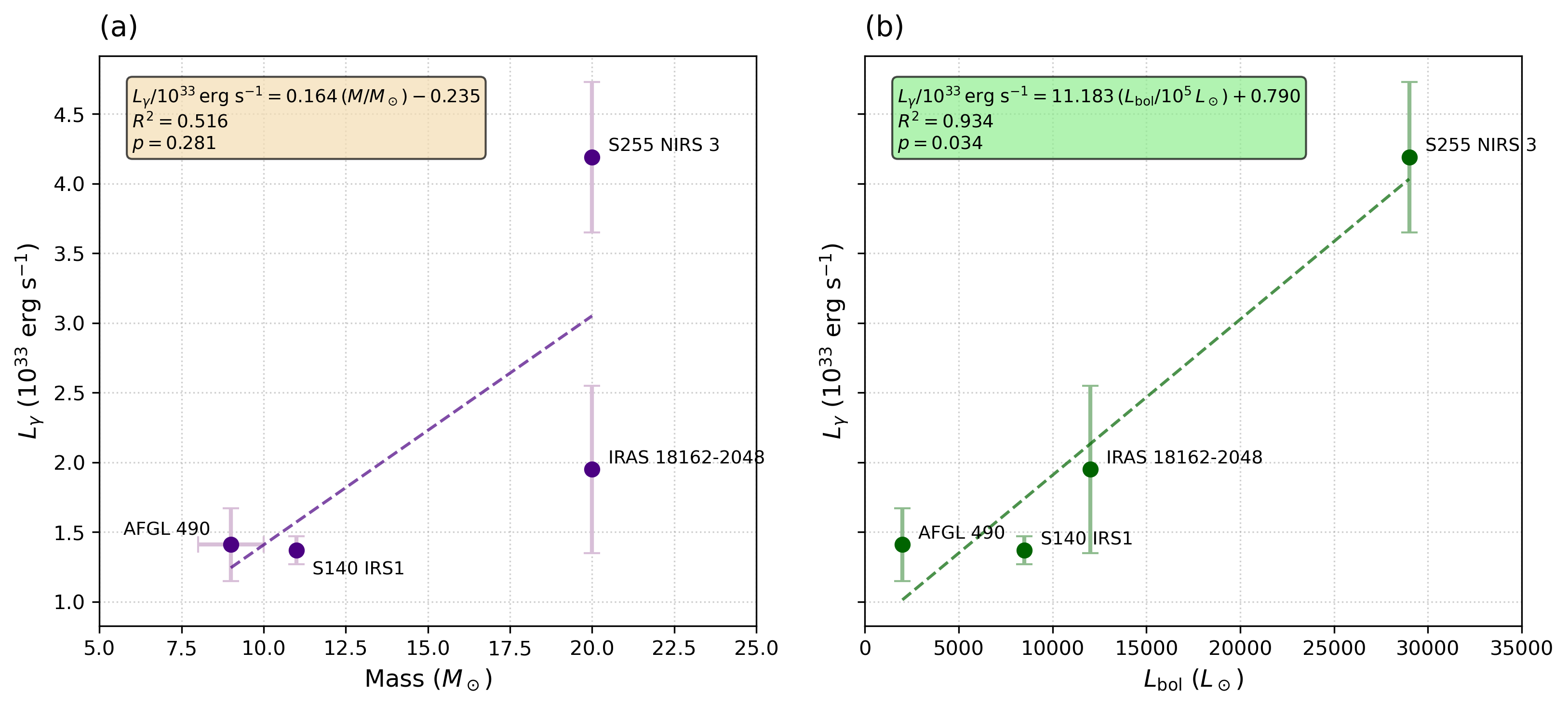
Finally, we compile the known (or candidate) cases of $\gamma$-ray emission from protostellar jets reported so far (see Sec. I) and compare them with S140 IRS1; the results are summarised in Tab. 4 and Fig. 4. A notable quantity is $L_{\gamma}/L_{\rm bol}$ ($\times 10^{5}$): HH 80-81, S255 NIRS3, and S140 IRS1 all exhibit values around 4, whereas AFGL 490 shows a significantly higher value of $\sim$18.

A linear regression analysis reveals that $L_{\gamma}$ exhibits no significant correlation with the source mass ($R^{2}=0.516$, $p=0.281$). In contrast, a tight positive correlation is found between $L_{\gamma}$ and $L_{\mathrm{bol}}$ ($R^{2}=0.934$, $p=0.034$), suggesting that the $\gamma$-ray luminosity primarily scales with the overall energy output rather than the final stellar mass. However, given the extremely limited sample size of only four sources, this preliminary correlation is statistically fragile and cannot be generalized as a universal physical law at present. Dedicated observations targeting protostellar objects across a wider range of bolometric luminosities are necessary to robustly verify this physical association.

To gain further physical insight into the underlying mechanisms, we can decompose this ratio using the following expression:

where the term $L_{\mathrm{acc}}/L_{\mathrm{bol}}$ characterizes the accretion intensity of massive protostars, representing the proportion of bolometric luminosity driven by ongoing accretion. The main difficulty in estimating this ratio stems from the considerable uncertainty in determining $L_{\mathrm{acc}}$. Among the three known $\gamma$-ray emitting protostellar systems mentioned above, this ratio can only be evaluated for AFGL 490 ($\sim 42.5\%$) (Yang et al., 2026), while it reaches $\sim 62.4\%$ for S140 IRS1. For IRAS 18162–2048 (HH 80-81), no estimate of $L_{\mathrm{acc}}$ is available, and for S255 NIRS 3, only the $L_{\mathrm{acc}}$ during the outburst phase is known, rather than in quiescence. Next, the term $L_{\mathrm{jet}}/L_{\mathrm{acc}}$ describes the fraction of accretion energy converted into the kinetic power of the jet, potentially associated with certain magnetohydrodynamic (MHD) processes. For example, Cabrit (2007) reported $L_{\mathrm{jet}}/L_{\mathrm{acc}}\sim 7.5\%$, which is the value adopted in this work. Finally, the term $L_{\gamma}/L_{\mathrm{jet}}$ represents the efficiency with which the jet’s kinetic energy is converted into $\gamma$-ray luminosity, which currently stands as the parameter about which we have the most limited understanding.