Bag-of-Visual-Words for Spatial Mapping of Lung Adenocarcinoma Growth Patterns††thanks: Supported by the Swiss National Science Foundation (SNSF) under Grant No. 220761
Abstract
Spatial mapping of lung adenocarcinoma (LUAD) growth patterns across whole slide images (WSIs) requires resolving architectural context at the region level, yet existing methods operate at the individual tile level and produce generic morphological clusters rather than clinically defined pattern maps. We propose a weakly supervised Bag-of-Visual-Words (BoVW) pipeline that learns a visual vocabulary from frozen foundation model embeddings extracted from a small set of annotated regions of interest (ROIs). Pattern prototypes are constructed as mean BoVW histograms of same-label ROIs and used for nearest-prototype classification of sliding-window regions under Jensen–Shannon divergence. The resulting predictions are projected onto the WSI tile grid to produce interpretable spatial pattern maps. We evaluate the method on 87 CPTAC-LUAD patients using three foundation model encoders and multiple vocabulary sizes on two clinically motivated tasks. For tumour/healthy classification, the best configuration achieves a balanced accuracy of with H-Optimus-1, approaching the obtained by a supervised SVM trained on mean-pooled WSI embeddings. For binary histologic grade classification, the BoVW pipeline achieves higher balanced accuracy than the supervised baseline for all encoders, suggesting that ROI-level pattern decomposition preserves grade-relevant heterogeneity that is attenuated by global mean pooling.
1 Introduction
Lung adenocarcinoma (LUAD) is characterised by a diverse set of histological growth patterns, namely lepidic, acinar, papillary, micropapillary, and solid, whose spatial distribution within a tumour carries significant prognostic information [1]. In clinical practice, pathologists report the dominant growth pattern per whole slide image (WSI), a convention that obscures the intratumoural heterogeneity that is increasingly recognised as a determinant of disease progression and treatment response. Spatial maps showing the distribution of growth patterns across a WSI would provide clinicians with richer information than a single dominant label, enabling quantitative characterisation of pattern composition and heterogeneity at the slide level. Yet the computational tools to generate such maps remain limited.
The challenge concerns both supervision and spatial scale. Prior supervised approaches have used pixel-wise semantic segmentation [2] or patch-level classification across WSIs [3, 4]. However, dense pixel annotations are costly and arguably finer than required for regionally defined LUAD growth patterns, while independent patch predictions capture only limited architectural context. Existing datasets such as ANORAK [2] instead annotate selected ROIs, whereas larger weakly labelled cohorts typically provide only a dominant slide label. These limitations motivate ROI-level spatial mapping from limited regional supervision.
Unsupervised methods have emerged as a promising alternative. Histomorphological Phenotype Learning (HPL) [5] and PANTHER [6] demonstrate that self-supervised tile embeddings can be clustered into morphologically coherent phenotype groups, producing spatial maps of tissue composition without any annotation. However, these methods operate at the individual tile level, typically pixels, and discover generic morphological concepts rather than the specific WHO-defined LUAD growth patterns. This is a fundamental limitation: LUAD growth patterns are architectural phenomena defined by the spatial arrangement of cells across multiple tile widths. A lepidic pattern is recognisable from the preservation of alveolar architecture across a region, not from any single tile in isolation. Tile-level clustering conflates locally similar tiles that belong to architecturally distinct patterns, reducing discriminability for the clinically relevant pattern taxonomy.
We adopt the region of interest (ROI) as the unit of analysis for LUAD growth pattern mapping. This is motivated by how pathologists annotate these patterns in practice: annotation protocols instruct experts to delineate regions as large as possible that are relatively pure, containing a single pattern [7, 2]. Furthermore, growth patterns are defined by the spatial arrangement of cells across a tissue region rather than by local pixel features [7], and empirical studies show that pattern recognition benefits from a field of view spanning several hundred microns [7]. An ROI spanning multiple tile widths therefore captures the architectural context required to identify each pattern, while remaining far coarser than pixel-level segmentation and computationally tractable at the WSI scale.
In this paper we propose a weakly supervised pipeline for spatial LUAD growth pattern mapping that operates at the ROI level. A visual vocabulary is learned by clustering tile embeddings from 168 annotated ROIs using a frozen foundation model encoder, and per-pattern prototypes are constructed as mean BoVW histograms of same-label ROIs. Pattern assignment on unseen WSIs is performed by nearest-prototype retrieval under Jensen–Shannon Divergence, and predictions are assembled into spatial pattern maps on the WSI tile grid. Evaluated on CPTAC-LUAD WSIs on tumour/healthy classification and binary histologic grade classification, our method achieves balanced accuracies of and respectively, with the latter outperforming a directly supervised baseline ().
2 Method
We propose a weakly supervised pipeline for spatially mapping LUAD growth patterns across WSIs. Given a small set of pattern-labelled regions of interest (ROIs) and a collection of unannotated whole slide images (WSIs), the goal is to assign a growth pattern label to every spatial position of each WSI without tile-level or pixel-level supervision. The pipeline proceeds in four stages: (i) visual vocabulary learning from annotated ROI tiles, (ii) ROI histogram encoding, (iii) per-pattern prototype construction, and (iv) WSI pattern assignment and spatial mapping, as illustrated in Figure 1.

2.1 Visual Vocabulary Learning
Let denote the set of -normalised tile embeddings extracted from all annotated ROIs using a frozen foundation model encoder . Although individual tiles carry no label, they are drawn exclusively from tissue regions whose enclosing ROI has been assigned a pattern label.
A visual vocabulary of visual words is learned by applying -Means to the embeddings of tiles extracted from the annotated ROIs (stages I and II in Figure 1):
| (1) |
yielding centroids that constitute the vocabulary. The algorithm operates without access to pattern labels, making vocabulary construction entirely unsupervised.
2.2 ROI Histogram Encoding
Given the vocabulary of centroids, each annotated ROI is encoded as a normalised histogram over visual words, the Bag-of-Visual-Words (BoVW) representation [8, 9]. For the tile embeddings belonging to ROI , each tile is assigned to its nearest centroid:
| (2) |
Because all embeddings and centroids are -normalised and therefore lie on the unit hypersphere, minimising squared Euclidean distance is equivalent to maximising cosine similarity: . The assignment in Eq. (2) thus selects the visually most similar visual word for each tile.
The ROI histogram is formed as the mean of one-hot assignment vectors:
| (3) |
where is the one-hot indicator of word . By construction is -normalised and constitutes a valid discrete probability distribution over the visual words.
2.3 Per-Pattern Prototype Construction
Let denote the set of BoVW histograms of all annotated ROIs carrying label , where Lepidic, Acinar, Papillary, Micropapillary, Solid, Normal. The prototype of pattern is the mean BoVW histogram over all ROIs of that pattern:
| (4) |
Because each histogram is already -normalised, is itself a valid probability distribution.
Vocabulary quality criterion.
The separability of the learned prototypes is assessed by computing the full matrix of pairwise Jensen–Shannon Divergences (JSD) between all prototype pairs. For two distributions :
| (5) |
where is the KL divergence. JSD is symmetric, bounded in , and well-defined even when histograms contain zero-count bins (a small smoothing constant is applied). A vocabulary passes quality control if , where is the threshold below which two prototypes are considered effectively indistinguishable.
2.4 WSI Pattern Assignment and Spatial Mapping
Sliding-window ROI extraction.
Pattern assignment.
Each WSI-ROI is assigned the pattern whose prototype is closest under JSD (Eq. (5)):
| (6) |
Spatial mapping.
ROI predictions are projected back onto the WSI tile grid (stage IV in Figure 1). Classification confidence for each ROI is defined as the normalised margin between the JSD distances to the closest and second-closest prototypes, , where and denote the closest and second-closest prototype distances respectively. ROIs whose confidence falls below threshold are labelled Unknown; each Unknown ROI is then relabelled by majority vote over its immediate grid neighbours, exploiting the spatial contiguity of LUAD growth patterns.
WSI-level classification tasks.
Two downstream tasks are evaluated.
Task 1: tumour/healthy classification. A WSI is classified as tumour if at least one ROI prediction belongs to a cancer pattern (); otherwise it is classified as healthy.
Task 2: binary histologic grade classification. High-grade patterns (Solid, Micropapillary) are associated with worse survival and higher recurrence risk than low-grade patterns (Lepidic, Acinar, Papillary) [1, 10, 11]. Each patient is assigned a binary grade from their ROI-level predictions using a highest-grade-wins rule, consistent with IASLC recommendations [1]:
| (7) |
3 Experiments and Results
We evaluate the pipeline on 87 CPTAC-LUAD [12] patients comprising 453 WSI entries, using H-Optimus-1 [13], H0-Mini [14], and UNI2-h [15], with vocabulary sizes . All analyses use -pixel tiles at magnification, matching the native input configuration of the encoders.
The reference pool contains 168 pattern-enriched ROIs of pixels, corresponding to 6,048 tiles. ROIs were selected from CPTAC-LUAD slides with dominant-pattern metadata. A pretrained tumour-localisation model was used only to identify tumour tissue, after which ROIs were manually selected by a computational pathology researcher without formal pathology training using the slide metadata and published morphological criteria. These ROIs are used exclusively for vocabulary learning and prototype construction. Evaluation patients are disjoint from those contributing reference ROIs.
Sliding-window regions extracted during WSI inference use the same size pixel field of view. Results are reported for WSI-level tumour/healthy classification and patient-level binary histologic grade classification. The supervised baseline mean-pools tile embeddings within each region and region embeddings within each WSI, followed by an SVM evaluated using leave-one-patient-out cross-validation. In contrast, the BoVW prototypes are learned from the disjoint reference ROI pool and applied without fitting to labels from the evaluation cohort. Attention-based multiple instance learning [16] was not evaluated because the labelled cohort was considered insufficient for reliable training.
3.1 Vocabulary Evaluation
Inter-prototype separability.
Table 1 reports the inter-prototype JSD matrix for H-Optimus-1 at . The lowest separation is between Acinar and Papillary, reflecting their known architectural similarity as glandular patterns [17]. The highest separation is between Micropapillary and Lepidic, consistent with these patterns representing opposite ends of the LUAD architectural spectrum. Table 2 shows that H-Optimus-1 achieves consistently higher minimum JSD than H0-Mini, while UNI2-h attains the highest absolute minimum yet underperforms on downstream classification (Tables 3 and 4), suggesting prototype separability is necessary but not sufficient for WSI-level pattern mapping. At , vocabulary size equals the number of pattern classes, yielding by construction due to trivially disjoint prototypes; these values are excluded from the trend analysis. For all encoders, minimum JSD increases monotonically with , yet the vocabulary size that maximises separability differs from the one that maximises classification accuracy. Every (encoder, ) configuration evaluated satisfies the quality criterion of Section 2.3 (, excluding the degenerate case), so no vocabulary was excluded from the downstream evaluation on this basis.
| Acin. | Lepi. | Microp. | Pap. | Solid | Norm. | |
|---|---|---|---|---|---|---|
| Acinar | — | 0.994 | 0.940 | 0.741 | 0.746 | 0.976 |
| Lepidic | 0.994 | — | 0.996 | 0.855 | 0.993 | 0.967 |
| Micropap. | 0.940 | 0.996 | — | 0.924 | 0.940 | 0.945 |
| Papillary | 0.741 | 0.855 | 0.924 | — | 0.955 | 0.991 |
| Solid | 0.746 | 0.993 | 0.940 | 0.955 | — | 0.929 |
| Normal | 0.976 | 0.967 | 0.945 | 0.991 | 0.929 | — |
| Encoder | |||||
|---|---|---|---|---|---|
| H-Optimus-1 | 0.741 | 0.752 | 0.785 | 0.825 | |
| H0-Mini | 0.469 | 0.516 | 0.506 | 0.545 | |
| UNI2-h | 0.824 | 0.844 | 0.830 | 0.910 | |
| †Degenerate case: disjoint support by construction. | |||||
3.2 Spatial Pattern Maps
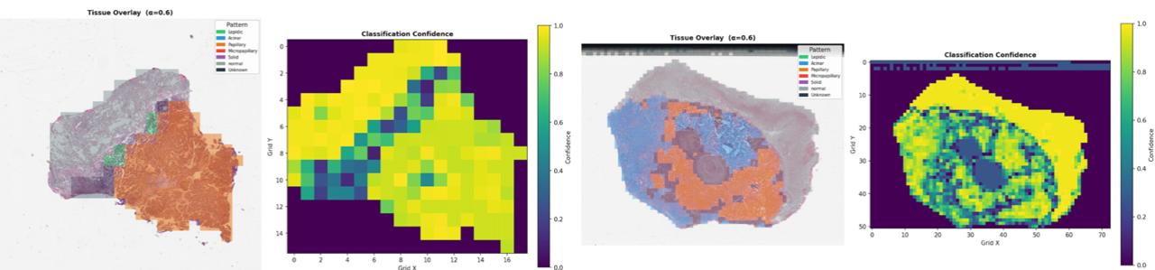
Each sliding-window ROI is coloured by and placed at its centre coordinates in tile units, with the confidence threshold set to and confidence encoded in a complementary heatmap. Representative maps for two CPTAC-LUAD slides are shown in Figure 2 (H-Optimus-1, ). Both slides show spatially coherent pattern regions consistent with expected tissue architecture, and uncertainty concentrates at pattern boundaries rather than being randomly distributed. This qualitative visual inspection suggests that the pipeline recovers plausible pattern organisation; a formal assessment by pathologists is left to future work (see Section 4).
3.3 Downstream Classification
Task 1: tumour/healthy classification.
The BoVW pipeline using H-Optimus-1 and H0-Mini both peak at , while UNI2-h improves monotonically with , peaking at , substantially below the other two encoders (Table 3). The small gap between the supervised baseline and the best BoVW configurations ( for H-Optimus-1) indicates that the training-free prototype pipeline achieves near-parity with a directly supervised method for tumour detection, a task for which the embedding signal is strong across all encoders.
Task 2: binary histologic grade classification.
The BoVW pipeline achieves higher balanced accuracy than the supervised SVM baseline for all three encoders (Table 4), with H-Optimus-1 at yielding the highest BoVW performance. This consistent advantage across encoders demonstrates that distributing WSI representation over pattern-relevant visual words preserves grade-discriminative spatial heterogeneity that is lost when embeddings are mean-pooled to a single vector. Notably, the optimal for Task 2 () is coarser than for Task 1 (), indicating that grade discrimination and tumour detection impose different requirements on vocabulary granularity. Task 2 results should be interpreted with caution given the cohort imbalance (68 low-grade, 19 high-grade), and validated on larger, balanced datasets.
| Healthy | Tumour | |||||||
|---|---|---|---|---|---|---|---|---|
| Encoder | Bal.Acc | P | R | F1 | P | R | F1 | |
| H-Optimus-1 | 6 | 0.738 | 1.00 | 0.48 | 0.64 | 0.77 | 1.00 | 0.87 |
| 8 | 0.955 | 0.99 | 0.91 | 0.95 | 0.95 | 1.00 | 0.97 | |
| 12 | 0.765 | 1.00 | 0.53 | 0.69 | 0.79 | 1.00 | 0.88 | |
| 16 | 0.974 | 0.99 | 0.95 | 0.97 | 0.97 | 1.00 | 0.98 | |
| 18 | 0.795 | 0.99 | 0.59 | 0.74 | 0.81 | 1.00 | 0.90 | |
| Baseline | 0.987 | 0.99 | 0.98 | 0.98 | 0.99 | 0.99 | 0.99 | |
| H0-Mini | 6 | 0.818 | 1.00 | 0.64 | 0.78 | 0.83 | 1.00 | 0.91 |
| 8 | 0.827 | 1.00 | 0.65 | 0.79 | 0.84 | 1.00 | 0.91 | |
| 12 | 0.858 | 0.98 | 0.72 | 0.83 | 0.87 | 0.99 | 0.92 | |
| 16 | 0.955 | 0.99 | 0.91 | 0.95 | 0.95 | 1.00 | 0.97 | |
| 18 | 0.921 | 0.99 | 0.85 | 0.91 | 0.92 | 1.00 | 0.96 | |
| Baseline | 0.981 | 0.98 | 0.98 | 0.98 | 0.99 | 0.99 | 0.99 | |
| UNI2-h | 6 | 0.698 | 1.00 | 0.40 | 0.57 | 0.75 | 1.00 | 0.86 |
| 8 | 0.694 | 1.00 | 0.39 | 0.56 | 0.75 | 1.00 | 0.85 | |
| 12 | 0.775 | 1.00 | 0.55 | 0.71 | 0.80 | 1.00 | 0.89 | |
| 16 | 0.788 | 0.99 | 0.58 | 0.73 | 0.81 | 1.00 | 0.89 | |
| 18 | 0.810 | 0.99 | 0.62 | 0.77 | 0.83 | 1.00 | 0.90 | |
| Baseline | 0.984 | 0.99 | 0.98 | 0.98 | 0.99 | 0.99 | 0.99 | |
| Low-grade | High-grade | ||||||||
|---|---|---|---|---|---|---|---|---|---|
| Encoder | Bal.Acc | Mac.F1 | P | R | F1 | P | R | F1 | |
| H-Optimus-1 | 6 | 0.707 | 0.641 | 0.90 | 0.68 | 0.77 | 0.39 | 0.74 | 0.51 |
| 8 | 0.729 | 0.671 | 0.91 | 0.72 | 0.80 | 0.42 | 0.74 | 0.54 | |
| 12 | 0.714 | 0.651 | 0.90 | 0.69 | 0.78 | 0.40 | 0.74 | 0.52 | |
| 16 | 0.714 | 0.651 | 0.90 | 0.69 | 0.78 | 0.40 | 0.74 | 0.52 | |
| 18 | 0.714 | 0.651 | 0.90 | 0.69 | 0.78 | 0.40 | 0.74 | 0.52 | |
| Baseline | 0.678 | 0.685 | 0.86 | 0.88 | 0.87 | 0.53 | 0.47 | 0.50 | |
| H0-Mini | 6 | 0.685 | 0.612 | 0.90 | 0.63 | 0.74 | 0.36 | 0.74 | 0.48 |
| 8 | 0.692 | 0.622 | 0.90 | 0.65 | 0.75 | 0.37 | 0.74 | 0.49 | |
| 12 | 0.673 | 0.615 | 0.88 | 0.66 | 0.76 | 0.36 | 0.68 | 0.47 | |
| 16 | 0.651 | 0.586 | 0.88 | 0.62 | 0.72 | 0.33 | 0.68 | 0.45 | |
| 18 | 0.666 | 0.605 | 0.88 | 0.65 | 0.75 | 0.35 | 0.68 | 0.46 | |
| Baseline | 0.644 | 0.650 | 0.84 | 0.87 | 0.86 | 0.47 | 0.42 | 0.44 | |
| UNI2-h | 6 | 0.699 | 0.631 | 0.90 | 0.66 | 0.76 | 0.38 | 0.74 | 0.50 |
| 8 | 0.692 | 0.622 | 0.90 | 0.65 | 0.75 | 0.37 | 0.74 | 0.49 | |
| 12 | 0.699 | 0.631 | 0.90 | 0.66 | 0.76 | 0.38 | 0.74 | 0.50 | |
| 16 | 0.707 | 0.641 | 0.90 | 0.68 | 0.77 | 0.39 | 0.74 | 0.51 | |
| 18 | 0.707 | 0.641 | 0.90 | 0.68 | 0.77 | 0.39 | 0.74 | 0.51 | |
| Baseline | 0.693 | 0.708 | 0.86 | 0.91 | 0.89 | 0.60 | 0.47 | 0.53 | |
4 Discussion
Our results show that a training-free BoVW pipeline anchored to a small set of reference ROIs can produce spatially coherent LUAD growth-pattern maps and competitive downstream classification. For binary grade classification, the BoVW pipeline achieves higher balanced accuracy than the supervised SVM baseline across all three encoders. This comparison should nevertheless be interpreted with care, since the SVM is trained through leave-one-patient-out cross-validation on the evaluation cohort, whereas the BoVW prototypes are learned from a disjoint reference set. The results suggest that decomposing each WSI into pattern-relevant visual words may preserve the contribution of spatially limited high-grade regions that can be attenuated by global mean pooling.
The two tasks benefit from different levels of vocabulary granularity, reflecting the different nature of the discriminative signal: separating tumour from healthy tissue relies on coarser tissue-type differences, while grade discrimination requires the vocabulary to resolve finer architectural distinctions between pattern groups.
Limitations.
Two data constraints limit the current study. The annotated ROI pool is small and class-imbalanced (14 to 44 ROIs per pattern), which may limit prototype quality for rare patterns. The evaluation dataset carries weak patient-level grade labels with no WSI-level ground truth and pronounced class imbalance (68 low-grade, 19 high-grade), which motivated the choice of binary rather than per-class evaluation and limits the conclusions that can be drawn from high-grade F1 values. Despite these constraints, the consistent advantage of the BoVW pipeline over the supervised baseline across all encoders and the qualitative coherence of the spatial maps suggest that the method is promising. Future work will leverage higher-quality hospital data to enable a more rigorous evaluation of per-class spatial mapping accuracy.
References
- [1] Moreira, A.L., et al.: A grading system for invasive pulmonary adenocarcinoma: a proposal from the International Association for the Study of Lung Cancer Pathology Committee. J. Thorac. Oncol. 15(10), 1599–1610 (2020).
- [2] Pan, X., AbdulJabbar, K., Coelho-Lima, J., et al.: The artificial intelligence-based model ANORAK improves histopathological grading of lung adenocarcinoma. Nature Cancer 5(2), 347–363 (2024).
- [3] Wei, J.W., Tafe, L.J., Linnik, Y.A., Vaickus, L.J., Tomita, N., Hassanpour, S.: Pathologist-level classification of histologic patterns on resected lung adenocarcinoma slides with deep neural networks. Sci. Rep. 9, 3358 (2019).
- [4] Lami, K., et al.: Standardized classification of lung adenocarcinoma subtypes and improvement of grading assessment through deep learning. Am. J. Pathol. 193(12), 2066–2079 (2023).
- [5] Quiros, A.C., Coudray, N., Yeaton, A., et al.: Mapping the landscape of histomorphological cancer phenotypes using self-supervised learning on unannotated pathology slides. Nature Commun. 15, 4596 (2024).
- [6] Song, A.H., Chen, R.J., Ding, T., et al.: Morphological Prototyping for Unsupervised Slide Representation Learning in Computational Pathology. arXiv:2405.11643 (2024).
- [7] Reisenbüchler, D., et al.: CellOMaps: A Compact Representation for Robust Classification of Lung Adenocarcinoma Growth Patterns. arXiv:2501.08094 (2025).
- [8] Sivic, J., Zisserman, A.: Video Google: A text retrieval approach to object matching in videos. In: ICCV, pp. 1470–1477 (2003).
- [9] Caicedo, J.C., Cruz, A., Gonzalez, F.A.: Histopathology image classification using bag of features and kernel functions. In: AIME, pp. 126–135 (2009).
- [10] Travis, W.D., et al.: The 2015 World Health Organization Classification of Lung Tumors. J. Thorac. Oncol. 10(9), 1243–1260 (2015).
- [11] Sica, G., et al.: A grading system of lung adenocarcinomas based on histologic pattern is predictive of disease recurrence in stage I tumors. Am. J. Surg. Pathol. 34(8), 1155–1162 (2010).
- [12] Edwards, N.J., et al.: The CPTAC Data Portal: A Resource for Cancer Proteomics Research. J. Proteome Res. 14(6), 2707–2713 (2015).
- [13] Scalbert, M., Saillard, C., Peeters, T., et al.: H-optimus-1: A foundation model for computational histopathology. In: Proc. AACR Annual Meeting, Cancer Research 86(8_Suppl), LB174 (2026).
- [14] Filiot, A., Dop, N., Tchita, O., et al.: Distilling foundation models for robust and efficient models in digital pathology. arXiv:2501.16239 (2025).
- [15] Chen, R.J., Ding, T., Lu, M.Y., et al.: Towards a general-purpose foundation model for computational pathology. Nature Medicine (2024).
- [16] Ilse, M., Tomczak, J., Welling, M.: Attention-based deep multiple instance learning. In: ICML, pp. 2127–2136 (2018).
- [17] Thunnissen, E., et al.: Reproducibility of histopathological subtypes and invasion in pulmonary adenocarcinoma. Mod. Pathol. 25(12), 1574–1583 (2012).