newfloatplacement\undefine@keynewfloatname\undefine@keynewfloatfileext\undefine@keynewfloatwithin
Quantifying Different Gains from Trade in Quality
Abstract
In this paper, I study to what extent countries differ in their preferences for quality and their technologies for improving quality. The paper also quantifies the contribution of those differences to the differences in gains from trade across countries. I adopt [undefc], which allows endogenous quality choice of firms. This paper extends that framework into multi-country and multi-sector setting. The new feature is that bilateral trade liberalization yields spillover effects on the competitiveness of another country. This paper structurally estimates the model under multi-country and multi-sector framework. It is found that richer countries generally have stronger valuation for quality. The quantification demonstrates that variations in the strength of quality preferences and in the technology of improving quality across countries add to their heterogeneities in market competitiveness. Subsequently, I simulate a 5% increase in the trade barriers. If the quality channel is shut down, countries with stronger preferences for quality have larger degrees of underestimations in their losses from the trade barrier. Finally, gains from a universal rise in quality preference are unequal among countries, with larger economies generally gaining more than smaller economies.
1 Introduction
Trade economists have paid particular attention to the role played by product quality in international trade. Under quality sorting, more efficient firms produce higher-quality goods, enter more competitive markets and charge higher prices,222See, for example, [undefe], [undeff], [undefj], [undefk] and [undefl]. which enriches conventional efficiency-based trade theories.333Conventional heterogeneous firm trade theories include [undefal] and [undefam]. Additionally, quality differentiations across firms and markets can explain price variations in exports and imports.444See, for example, [undefaf]. Finally, the product quality is related to welfare gains from trade.555See, for example, [undefo]
This paper analyzes differences in quality preferences and technologies among countries and investigates the impact of these differences on gains from trade. Despite the growing literature linking quality, price and welfare, little has considered the contribution of quality either to cross-country differences in market competitiveness or to unequal gains from trade. In addition, this paper is the first to quantify the countries’ heterogeneities in quality preferences and costs from both demand and supply sides. In this paper, I investigate this problem using a combination of empirical, theoretical and structural analyses. Two findings emerge from this analysis: first, differences in quality preferences among countries enlarge the inequality in gains from trade; second, a universal rise in quality preferences brings higher gains to larger economies.
To provide micro-foundations, I use a recent Chinese firm-level export transaction dataset to explore firm-level evidence. Evidence from this dataset shows that firms charging higher prices sell to larger countries, earn higher revenues and enter more markets. The positive relationship between price, revenue, and market entry is strengthened in sectors of high research and development (R&D) intensity. Typically, R&D intensity can be viewed as a proxy for scope of quality differentiation in [undefah]. Additionally, I choose two sectors with different levels of R&D intensity - tobacco (R&D intensity approximately zero) and pharmaceutical (R&D intensity approximately 50%). In the pharmaceutical sector, the positive relationship between price, revenue and market entry still holds. However, in tobacco sector, price is negatively correlated to revenue and the destination market size. The evidence reveals that the price is positively correlated destination market size, firm revenues and market entry in a subset of sectors only. This implies that price reveals quality only in selected industries and that some sectors are homogeneous with limited quality differentiation space.
Motivated by these stylized facts, I extend the framework of [undefc] into the multi-country and multi-sector setting. The framework introduces quality differentiation into [undefam] (MO, thereafter). According to [undefc], firms compete along the quality dimension as well as cost dimension so that more productive firms charge higher prices because they can produce higher-quality products. I also extend [undefc] so that a firm can produce multiple products. The extension suggests that more productive firms produce more products with higher average qualities. On the demand side, quality preferences are homogeneous within a country and sector. On the supply side, the cost of improving quality is embedded in both variable and sunk costs that firms have to pay.
In the multi-country setting in this paper, it is possible to assess spillover effects of the bilateral trade liberalization and the preference shock. The spillover effect is unique to this multi-country model. A bilateral trade liberalization between two countries can generate negative effect on competitiveness of other countries. The effect on the third country is higher, the larger the trade-liberalizing economies. Apart from that, a positive preference shock on one country could have positive effect on competitiveness of other countries. This occurs since quality differentiation scope in selling to that market are widened following positive preference shock. Firms in all countries respond by rising quality of goods sold to that market. The responses are higher for more productive firms. Therefore, the productivity threshold of entering the market with preference shock rises. As for other countries without shocks, the least productive firms cannot profitably export to the market with the positive preference shock. This makes this group of firms unable to cover the sunk cost of entry. Thus, the least productive firms are driven out of the market, in all countries. The productivity thresholds of other countries without preference shock could also rise. The larger the country with preference shock, the higher the effects on productivity of other countries. Finally, if the trade liberalization negatively affect competitiveness of a third country, higher quality preference alleviate the negative effect. If the trade liberalization positively affect competitiveness of a third country, higher quality preference strengthen the positive effect. This occurs since higher quality preference have positive selection effect.
The multi-country setting of this paper enables computation of equilibrium. I bring the model to data to estimate the relevant parameters of quality in the model. An extended gravity model can be derived from the above theoretical framework. In addition to the bilateral trade costs and the importer/exporter fixed effects typically included in a gravity model estimation,666The original gravity model starts from [undefas] and is augmented by [undefa]. I include (a non-linear function of) quality preferences and costs into the the gravity equation. According to this gravity model, bilateral trade flow is positively affected by the destination country’s quality preferences and negatively affected by the origin country’s costs of improving quality.777The details of this are discussed in the Section 3 and Section 4. I parameterize that gravity equation to estimate quality preferences/costs parameters as well as trade costs. After the estimation, I recover two measures of the degree of competition for each country-sector pair. The first measure is endogenous competitiveness. This is the productivity threshold above which firms can make non-negative profits. Thus, before a firm makes a random draw of productivity, a firm will be, ex ante, less likely to enter a market where the cutoff productivity is high and competition is fierce. The second is the exogenous measure of competitiveness. This is the fundamental productivity level in a market. Firms are more likely to draw a high productivity if the level of fundamental productivity is higher. I follow [undefi] and estimate the endogenous competitiveness first and back out the exogenous competitiveness using free-entry conditions.888This is discussed in detail in Section 4.
The structural analysis suggests that quality preferences are related to income and that considering quality enlarges differences in competitiveness across countries. First, the preference for quality is positively correlated with GDP per capita in more than half of the sectors studied.999For the rest of sectors, GDP per capita has insignificant effect on quality preferences. This indicates that for these industries, the preferences for quality are on average stronger in richer countries. Second, the distribution of preferences for quality vary across sectors. The variance of the estimates across countries is particularly large for certain sectors such as HS 85 (Electrical machinery and equipment), which is 56.19, and small for certain sectors such as HS 37 (Photographic or cinematographic goods), which is approximately 9.94.101010As for the cost of quality, it is found that the mean is smaller than the preference parameters within the same sector and the variance are also smaller. These findings are, to some extent, consistent with empirical evidence on the correlation between price and market size.111111[undefar] among other, reports a negative correlation between market size and output price, while [undefau] and [undefx] report positive correlations. For example, [undefaa] and [undefab] finds that prices are a good proxy for quality in some industries but not in others. I compare the endogenous competitiveness estimated from this model with that estimated from the MO canonical model. Comparing across countries by sector, it is noticeable that endogenous competitiveness is more dispersed under this model. This more dispersed distribution can be explained by the additional heterogeneity introduced by differentials in both quality preferences and costs of improving quality among countries.
A counterfactual exercise is performed to examine the competitiveness-enhancing effect of quality. Exogenous competitiveness and quality parameters are kept constant. I experiment with a 5% universal increase in international trade costs. This exercise is implemented under both this model and the MO model. In general, the productivity cutoffs, which measure the endogenous competitiveness, decrease in both models. This implies that the average productivity is lower and the economy becomes less competitive. Quantitatively, the decline of the productivity cutoff is 25% to 300% larger in this model with quality than that it is in the MO setup (depending on the sector). Furthermore, the differences between this model and the MO model in degrees of the declines of productivity cutoffs rise in the magnitude of preferences for quality, in most sectors. If consumers value quality more in some countries, the difference between the rise of productivity cutoffs in this model and in the MO model will be larger in these countries than the difference in other countries where quality is not valued. This suggests that gains from trade across countries are more heterogeneous than in a canonical model, in which quality is considered.
For the second counterfactual exercise, I simulate a universal positive shock in preference for quality. Although quality preferences are exogenous to this model, they can change over time by promoting consumers’ awareness of product quality. Most countries experience gains in productivity of less than 141.2%. Approximately 25 countries experience a loss in productivity. The total gains in productivity is nearly 5 times the total losses in productivity, from the global scale. It is noticeable that large economies generally gain more than small economies. On average, 1% rise in population size leads to 7.876% more gains in productivity. This finding is consistent with the model implication that larger economies have wider scope for quality differentiation.
Quality in international trade has been intensively studied, but existing work pays limited attention to sources of quality variation from both the demand and the supply side and does not link them to heterogeneity among countries. [undefw] estimates the demand for quality across countries on the demand side. Other studies focus more on firms’ behavior in quality improvement ([undefg], among others). Nevertheless, [undefc] reconciles both the demand and the supply sides into a single theoretical framework. This paper uses a more general framework and compares predictive differences between that quality-extended model and the MO model.
The analysis of this paper provides new insight into the sources of unequal gains from trade from a quality perspective. That countries do not gain equally has been well documented. Gains from trade can be divergent among countries of different sizes ([undefai], among others) or incomes ([undefat], among others). A recent study by [undefb] suggests that free trade agreement (FTA) can bring -0.3% to 5% gains to different countries. However, little literature provides explanations for the unequal gains across countries. The paper points out and quantifies the strengthening effect on competition brought by higher quality preferences and quantifies it.
The paper relates to three strands of literature: heterogeneous firms’ quality choices, pricing-to-market and non-homothetic preferences. Trade liberalization induces firms’ quality-upgrading behavior ([undefp], among others). Larger plants have higher output prices and use more expensive materials [undefad].121212Other studies include [undefah]. This paper embraces the above findings by allowing quality choices to be endogenous to firms such that prices and markups vary with plant size and productivity. The model also includes findings by [undefq] that export unit values vary to a larger extent than quality-adjusted prices.131313[undefd] finds that price deviate from purchasing power parity. Finally, the study, by estimating quality preferences and relating to the country-level income, incorporates non-homothetic preferences proposed by [undefm].141414Similarly, [undefr] proposes that richer households consume higher-elasticity goods more thus leading to more trade flows between high income countries than between low-income ones.
The remainder of the paper is organized as follows. Section 2 uses firm-product level trade statistics to explore the relationship between price, market features and firm exporting performances. I use these statistics to show the micro foundations of the model. Section 3 lays out the theoretical framework under a multi-country and multi-product setting. Section 4 discusses the data and how relevant parameters are estimated. Section 5 implements the counterfactual analysis. Finally, Section 6 concludes.
2 Stylized Facts
2.1 Data
In order to document stylized facts regarding f.o.b. export prices across destinations and across firms within the same destination, I use a unique micro-level data and two sets of macro-level data. The specific micro dataset used here is the China Customs Trade Statistics (CCTS) issued in 2013 by The General Administration of Customs. The advantage of this dataset is that it is highly disaggregated in recording the import/exports of Chinese firms. Additionally, it records the prices of exports/imports, origins/destinations of imports/exports, the product (HS8) of the transaction, and the mode (ordinary or processing) of international trade. I use the CEPII-Dist dataset to obtain bilateral characteristics of destination countries and China. The Penn World Table dataset is used to obtain population of destination countries.
2.2 Empirical Findings
In this subsection, I report three stylized facts concerning export prices across destinations and across firms within destinations. Although the existing literature such as [undefah] has documented these findings, it is important to show that they hold in the more recent years. Moreover, these are the facts to be embraced in the model and that lay the micro foundation in the model setup.
On export prices across destinations — Based on the entire customs export data in 2013, Table 1 reports the regression results using (log) export prices as the dependent variable and destination country’s population as the main explanatory variable, controlling for destination’s GDP per capita and distance to China. Columns 1-2 use the prices at the firm-HS8-country level and Columns 3-4 use HS8-country level. The coefficients on (log) population in all specifications are significantly positive, suggesting that export prices increase with the destination’s market size, consistent with [undefah]. Thus, it is summarized as the following fact:
Stylized Fact 1: On average, firms set higher export prices for the same product in larger markets.
On export prices and revenues - Table 2 presents robust evidence that firms charging higher export prices earn greater revenues even within very narrowly defined destination-product markets. In Columns 1-2, I use prices at the firm-HS8-country level and Columns 3-4 I use prices at firm-product level. This relationship is highly statistically significant. Importantly, it is also markedly stronger for goods with greater scope for quality upgrading, as proxied by sectors’ R&D intensity compiled by [undefac]. The magnitudes and signs of estimated coefficients are relatively robust to different specifications and different level of aggregations. The elasticity of export prices with respect to revenues is 0.15. A doubling in firm sales in a given market is thus associated with 20% higher bilateral unit prices for the average product. That number is bigger for sectors with higher R&D intensity. This yields the following fact:
Stylized Fact 2: On average, firms charge higher prices simultaneously earn greater revenues in each destination. The correlation between price and revenue is higher in R&D intensive sectors.
On prices and market entry -As reported in Table 3, exporters that supply more countries systematically charge higher average prices (Columns 1-2). Firms selling to more destinations also exhibit greater price dispersion across importers (Columns 3-4). In this table, I use prices (or price dispersions) at firm-HS8 product level. These results are both largely enhanced by products with substantial potential for quality differentiation. As columns (2) and (4) show, the patterns are stronger for sectors with larger scope for quality differentiation, which is proxied by sectoral R&D intensity, defined as before. The finding is consistent with [undefag] and [undefah] which use earlier versions of CCTS. This finding suggests the following fact:
Stylized Fact 3: On average, exporters entering more destinations and offering a wider range of export prices charge higher prices. The correlation between price and market entry is higher in R&D intensive sectors.
One caveat is that the above relationships can be sector-dependent. The above relationship exist only in a subset of sectors. In Figure 1 and 2, I plot the above 3 stylized facts for sector HS 24 (Tobacco) and HS 6, respectively. The findings of the three stylized facts continue to hold in the sub-sample of HS 6, while they are reversed in HS 24. From Figure (1(a)), the average price decreases with destination market size. Firms charging higher prices earn lower revenues, as in Figure (1(b)). The relationship between the firm’s price charged and the number of market it entered (Figure (1(c))) is not as significant as in sector HS 6 (2(c)). The comparison suggests that competition improves quality in only a subset of sectors. This is also consistent with the Table (2) -(3) where the relationship between price, revenue and market entry are "more positive" in R&D intensive sectors. In sector 30 (Pharmaceuticals), the average R&D intensity is approximately 58% while that ratio of sector 24 is 0.
3 Theory
I lay out theoretical frameworks that incorporate endogenous quality choices in the linear demand system. The demand side features heterogeneous quality preferences among different countries; In addition, quality upgrading requires additional variable and fixed costs such that producers endogenously choose the level of quality in their products. The model is built on a multi-country basis for the convenience of quantification in subsequent empirical studies. For simplicity, sector notations are dropped as there are no interactions between them.
3.1 Setup
I follow the framework of [undefc] and [undefs], the preference of a consumer in country is represented as (1). This utility function has the advantage that the price/quantity are linear in quality preference
| (1) | |||||
where and are individual ’s consumption in numeraire and differentiated goods (in sector ) respectively. The quality of each variety is given by and the taste for quality by consumers in country in sector is . In the above utility function, is equivalent to the variety-specific taste shifter in [undefs].151515The difference between this paper and [undefs] is that the latter regard the shifter as the idiosyncratic term. If qualities of all varieties are zero or if the taste parameters are zero, the model becomes traditional [undefam] model. Finally, and capture the degree of substitution between each variety and the numeraire. The parameter measures the degree of differentiation between varieties. picks up the degree of preference for variety. Specifically, are assumed to be positive and differ across countries and sectors.
This generates a linear inverse demand function that depends on both quantity and quality:
| (2) |
where . By re-arranging (2) one can obtain the total demand in country of each variety:
| (3) |
where is the mean price over all varieties in country , is the mean quality over all varieties in . This form of preference over quantity and quality ensures that demand function is linear in price and quality.
On the supply side, firms have to incur costs in both production and quality improvements. For simplicity, labor is assumed to be the only factor of production. As with most heterogeneous firm trade models, firms have to pay a sunk cost before they draw the productivity (marginal cost of production). If a firm in country produce and sell to country , it should choose both the quantity and the quality of its product, given the total cost function:
| (4) |
where is the ice-berg trade cost from country to and is the quality level of goods sold from to . The first term implies that firms have to incur additional marginal cost of quality upgrading,which depends on both quality level and quality improving technology at origin country , when producing in country ; the second term picks up the fixed cost of improving quality. To generate closed form solutions, I assume that the fixed cost is a quadratic function of quality level. A more generalized function form in the fixed cost can be found in [undefp] in which CES preference is assumed. In the cost function (4), the marginal cost of upgrading quality differs across countries/sectors, since labor productivity are heterogeneous across countries. The multiplier in the fixed cost is assumed to be identical across countries, since the fixed costs of innovation across countries, which include high-skilled workers, tend to be homogeneous across countries.161616This assumption is made since the highly skilled labor migrate to regions where wages are high, according to [undefao]. Therefore the wage for high skilled workers tend to converge over time.
3.2 Firms’ Problem
For a firm (of marginal cost ) from country selling to each (potential) market , it chooses quantity and quality to maximize profit:
| (5) |
Given the demand structure, the quantity of goods sold from country to country satisfies a linear function with respect to price :
| (6) |
where is the cost threshold so that firms with marginal cost of production can sell to market and make non-negative profits. Equation (6) shows that demand is linear to both price and quality. This makes it convenient for later analysis in optimal pricing.
Given the demand function and the firms’ problem, the optimal price and quantity as a function of quality is linear in marginal cost171717Per unit trade cost does not depend on quality:
| (7a) | ||||
| (7b) | ||||
where is the cost-cutoff in country , above which firms cannot profitably sell in market . This is also the endogenous competitiveness of country (lower cutoff, more endogenous competition), which changes with factors such as ice-berg trade costs, quality parameters and market size. Thus, that the profit of selling to market can be re-written as
| (8) |
Solving for the first-order conditions for profit, the optimal quality choice to sell from to of firm is written as a decreasing function of marginal cost so that more productive firms offer higher quality within a market
| (9) |
where . As Equation (9) shows, the quality is linearly related to marginal cost . Consistent with other international trade in quality literature,181818For example, see [undefo] in which more productive firms offer higher quality products with lower quality-adjusted costs. for the same firm from country , it is expected to offer higher quality goods to larger markets and countries with higher taste for quality. Higher quality is also expected from countries with higher labor productivity in quality improvement (i.e., lower ). It is noticeable that at the first glance, a lower cutoff resulting from trade liberalization seems to have negative impact on quality updates. However, a lower cutoff indicates that the average marginal cost is also lower, since firms with marginal cost above the new cutoff exit the market. Since firm-level quality decreases with , the average quality of products sold in the economy rises. That effect is higher the larger quality differentiation scope .
Given optimal quality function in (9) and price/quantity functions, it is evident that price and quantity can be further expressed as
| (10a) | ||||
| (10b) | ||||
So the for each firm with marginal cost of production , the operating revenue of exporting from country to is:
| (11) |
Equation (10) and (11) implies that other things equal, more productive firms charge higher prices and earn greater revenues from each destination, if . This is consistent with Stylized 2 in the prior section.
The operating profit can be expressed as191919Following [undefc], the fixed cost of upgrading quality is also regarded as sunk since this model is not dynamic.:
| (12) |
Profit function in (12) implies that countries of higher quality preferences offer higher profits, all else being equal. This is related to the third stylized facts. From (12), more productive firms earn higher profits and earn non-zero profits in a larger set of markets.
This profit function is a quality-adjusted form of [undefam], in which profits are magnified by a term larger than one. This quality-adjusted term is key to the later empirical analysis.
3.3 Equilibrium
In equilibrium, the free entry condition of each country implies that the expected profit (earned from selling to each market) of a firm is zero. Such that that
| (13) |
where is the sunk cost a firm have to pay prior to entry. It is assumed to be positive and can vary across countries and sectors. Equation (13) implies that operating profit from all markets are expected to merely compensate for the sunk cost.
Following prior literature, it is assumed here that marginal cost draws follow Pareto distribution: so that firms draw the marginal cost from the range . The term is the exogenous competitiveness in market . Lower values indicates that a firm in country is more likely to draw a lower cost. The power governs the Pareto distribution dispersion: higher implies that the distribution of is more concentrated.
Given profit as in (12), one can re-write the equilibrium condition in (13) for country so that the summation of expected profit from each market equals the sunk cost paid.
| (14) |
The same equilibrium condition can be written for each country , in the matrix form. In the multi-country case, the vector of cost threshold for each country satisfies:
| (15) |
where matrix is the the "quality adjusted" matrix of trade freeness. If there are a total of countries, the dimension is . This matrix is represented as the following form:
It is noticeable that whether elements in are larger or smaller than one depends on the trade freeness, ’s and ’s. If trade cost is small (i.e., is larger) and is large, element can exceed one.
The matrix is of dimension and is the diagonal matrix of market size for each country :
The last term on the right-hand-side of (15) is the vector of cutoffs (to the power of ), with the element being . On the right hand side of Equation (15), is the vector of exogenous competitiveness (to the power ), with element being . Both and are of dimension .
By inverting matrix , cost threshold for each country can be computed as follows:
| (16) |
where is the determinant of matrix and is the cofactor of . A closer examination of the matrices and Equation (16) implies that higher market size leads to a lower calculated cutoff, all else being equal.202020This also holds under multi-product setting in Appendix A. If ice-berg trade cost is symmetric, i.e. , bilateral trade liberalization can have heterogeneous effects on cost cutoffs of different countries. Following this argument, bilateral trade liberalization can have negative externalities on countries without trade liberalization.
Proposition 1.
If ice-berg trade cost is symmetric, i.e. , the effect of a bilateral trade liberalization between and on cutoffs is not universal i.e. , such that and . Additionally, B such that , and , . The larger the trade liberalizing economies, the higher the effects on the cutoff of country .
Proof.
See Appendix B ∎
The intuition for the negative externalities is comparable to the special case of two-country world. It is driven by the long-term entry.In the long run, the market entries in trade-liberalizing economies rise. This drives up the competitiveness, i.e. the cost cutoff decrease as a result. For other countries without trade liberalization, the profit from selling to these markets are higher, relative to countries with trade liberalization. This results in decreased entries and higher cost threshold.
Another implication from (16) is on the effect of a preference shock, i.e. a change in , on cutoffs of countries.
Proposition 2.
The effects of a shock in preference for quality of any country on cutoffs are universal, i.e. B such that , . The larger the country with preference shock, the higher the effects on the cutoff of country
Proof.
See Appendix B ∎
The intuition for this lies in the selection effect. Quality differentiation scope in selling to that market are widened following positive preference shock. Firms in all countries respond by rising quality of goods sold to that market. The responses are higher for more productive firms. Therefore, the productivity threshold of entering the market with preference shock rises. As for other countries without shocks, the least productive firms cannot profitably export to the market with the positive preference shock. This makes this group of firms unable to cover the sunk cost of entry. Thus, the least productive firms are driven out of the market, in all countries. The productivity thresholds of other countries without any preference shock also rise.
Additionally, the average bilateral f.o.b price and trade value can be computed by aggregating over 212121Trade value is computed based on f.o.b price.
| (17) |
This is related to the first stylized fact, which links price with market size. From (17), one can observe that market size affect price both by decreasing the cost cutoff and by increasing the scope for quality differentiation. If the latter dominates, the relationship between price and market size is similar to Figure (2(a)), otherwise, it is closer to (1(a)).
The total trade value from to
| (18) |
where denotes the expected number of entrants in country . From Equation (17) and (18), the quality components have two effects: higher raises prices and reduces the trade values because of the additional (variable) costs incurred in manufacturing higher-quality goods in the origin country. Higher quality preferences in the destination country raise the willingness to pay and thus average price and trade value rise. Another countervailing effect is that, higher quality preferences drive down the cost cutoffs in the importing country thus to some extent lowering prices and values.
Finally, one can compute other aggregate variables, which are the number of varieties, entries, price indexes and welfare. The expected number of varieties in a country (i.e., the number of producers from domestic and abroad servicing market ) is similar to the M.O model multiplied by a quality-adjustment term that is negatively related to (of the market ) and positively affected by (of each sourcing country). That can be characterized as:
| (19) |
where . denotes the number of varieties sold from country to country . Equation (19) indicates that a higher preference for quality can be countervailing: can directly lower the number of varieties because it imposes higher requirements for the quality firms offer to market such that fewer firms can meet the high-quality requirement. On the other hand, higher quality preferences lower the cutoffs as is previously argued, which then encourages entry by raising average profits.
One can solve for the number of entrants by noting that the number of producers from origin to destinations depends on the exogenous competitiveness of the origin country and the cutoff in the destination country. Equation (19) can be used to solve for the number of entrants in each country. Notice that the number of bilateral varieties satisfies the following condition
For each country , the total number of varieties from each sourcing country should equal Equation (19), which can be represented in the following condition
| (20) |
Under the multi-country set-up, refer to M.O model, re-arranging (19) leads to the following condition:
| (21) |
If there are countries, has the dimension of and is the transpose of matrix :
The second term on the left hand side is the diagonal matrix of and is also dimension of written as
and the third term denotes the vector of entrants with dimension . The element is .
On the right-hand-side, matrix is of dimension and the element is
The average price in a market is obtained by aggregating over the average delivered price over destinations. Using the bilateral price in (17), it is implied that the (weighted) expected price levels in country are as follows:
| (22) |
where . From (22), similar argument can be applied: higher can lower the cutoff thus lowering the price index. However, this raises prices, since the consumers could have a higher willingness to pay for high quality.
Finally, the welfare in country is as follows:
| (23) | |||||
where the quality component is defined in the similar manner as previous. Other things equal, higher valuation on quality always raises welfare: it directly raises welfare by raising the utility obtained from consuming higher quality goods; it indirectly increases welfare by reducing the cost cutoff so that more productive firms enters and provide higher quality goods.222222The third term in the square bracket has the opposite effect compared with the first two terms. I attempted to compute the last term (multiplied by ) and found that its proportion to the total welfare is less than 5%.
The above derivations indicate that the existence of quality can be double-sides. The subsequent proposition argues that if the quality scope is high, the quality preference amplifies the effect of the trade cost change.
Proposition 3.
The larger the scope for quality differentiation , the more likely the selection effect of quality preference , i.e. smaller.
Proof.
See Appendix B. ∎
3.4 Discussion
The theory sketched above is based on linear demand, and it addresses the point of pricing-to-market. Specifically, it relates market toughness to the behavior of firms, and consequently, to the economic aggregates such as price index and welfare. In such a setting, market toughness operates through two channels: an increase in competition and an increase in the scope for quality differentiation. The theory identifies the second channel through which market toughness affects firms’ outcomes. An increase in market toughness (e.g., an increase in market size or a decrease in trade costs) raises the scope of quality differentiation because it makes it easier for firms to recover the fixed cost of innovation. Under such circumstances, each firm responds by raising quality, mark-ups, and prices. The (endogenous) relation between the scope of quality differentiation and market toughness is a key element of the model and constitutes an important deviation from past work.232323These include works using CES framework, for example [undefu], [undefaf] and [undefp], etc. For the most productive firms, quality, prices and profit rise as the innovation effect dominates the competition. These firms can earn positive profit from exporting to more competitive market. This features the advantages of exporters. The theory provides clarity on the relation between prices, productivity, market shares, and quality. In heterogeneous firms’ trade models, if no quality is present, these models predict a negative correlation between prices and productivity. However, if quality is present, and if higher quality indicates higher prices, then the correlation between prices and productivity, and (possibly) between prices and firm size becomes positive. Furthermore, since these models produce a quality sorting along the productivity axis, then the correlation between prices and quality is also positive.
The model is also connected to prior theoretical frameworks. For example, [undefo] modified CES utility by allowing positive baseline utility. The derived price is then positively related to the destination market’s income. Variable markup is implied by this modification. The slight difference from this model is that quality does not depend on market size. The implications of the model are also consistent with other forms of extensions of Melitz-Ottaviano under quality framework. For example, using slightly different extensions of the MO framework with quality, [undefh] confirms the dominance of the quality-enhancing effect of competition using French firm-level data.
Furthermore, the setting can be extended to multi-product case. For instance, [undefl] discovers that core products have lower costs so that firms have more incentives to invest in upgrading quality in these groups of products. I follow [undefaj] and extend the current framework by allowing firms to sell more than one product to a market.242424Details of setup and derivations are in Appendix A. The implications are isomorphic to this extension. Under this setup, it is concluded that higher product customization costs lead to a more competitive market. For individual firms, rising market competitiveness exerts a larger effect on quality improvements of products closer to the core.
4 Quantification
This section discusses the dataset used in the study and the methodologies to compute relevant parameters. I focus on sectors that are for final consumption, since producers and consumers can have different attitudes towards quality.252525Sectors for intermediate use, capital investment and final consumption are recognized by Broad Economic Classification (BEC) conversion. As there is no sectoral interaction here, I carry out estimations sector by sector. According to the theoretical model, the parameters to be estimated are as follows: 1) preference and cost for each country and sector ; 2) cutoffs (endogenous competitiveness) for each country/sector; and 3) cost upper-bound (exogenous competitiveness) . Finally, sector refers to HS 2 product level. As one step in the counterfactual analysis, I perform the quantification under quality model and M.O model.
These are the steps to estimate the model:
Step 1. Given the bilateral trade flow in the data, the bilateral trade cost can be estimated using aggregate bilateral trade flow in (18).
Step 2. Obtain the residuals from the first step estimation and compute preference for quality and cost of improving quality for each country , using Generalized Method of Moments.
Step 3. With the above set of parameters, the cost cutoff (endogenous competitiveness, ) of each country is projected using bilateral price in (17).
Step 4. With parameters from the above three steps,the exogenous competitiveness (multiplied by fixed cost ) can be computed from free entry condition in (15).
4.1 Data
The main dataset used here is the BACI world trade database provided by CEPII. The origin of the dataset is COMTRADE of the United Nations Statistical Division. The advantage of BACI data is that it reconciles records of both exporter and importer when there are inconsistencies in the transaction records from both sides ([undeft]). Thus, the dataset is more accurate since the reliability of the reported data of both exporter and importer are evaluated and cross-proofed. Another advantage is that the dataset is highly disaggregated: it reports the bilateral trade value and quantity at the HS6 level for more than 5,000 HS6 sectors.
To complement the dataset, I collect bilateral remoteness data to proxy for ice-berg trade cost. The major statistics is from GeoDist data compiled by CEPII. This dataset records bilateral information on distance, and other variables used in gravity equations to identify particular links between two countries. These variables include colonial relation, common languages, the contiguity ([undefak]). Further, data on bilateral regional trade agreement and bilateral common currency relations are collected from de Sousa. These variables are used to proxy bilateral ice-berg trade cost. Finally, I proxy market size by population and this dataset is from Penn World Table.
I obtain Pareto distribution parameter from a global firm-level database. Here I use Orbis dataset for this purpose. The ORBIS database (compiled by the Bureau van Dijk Electronic Publishing, BvD) is a commercial dataset, which contains administrative data on 130 million firms worldwide. ORBIS is an umbrella product that provides firm-level data covering approximately 100+ countries, both developed and emerging, since 2008. This dataset covers both public and private firms. I access the financial module to obtain firm-level variables. Following [undefz], I use total asset, employment and material cost (either recorded in the original dataset or imputed by subtracting the total cost of employees from the cost of goods sold) to estimate total factor productivity (TFP) at the firm level. To get , I regress firm ranking (in TFP) on (computed) firm productivity.262626I use [undefae] to compute TFP. In the sample of firms, the majority consists of manufacturing. This gives .
Prior to the empirical studies, some summary statistics for the feature of the data are displayed first. Table 4 reports the number of observations for each HS 2 sector. A small number of observations in one sector indicates that zero trade occur very frequently. It is implied that sectors are heterogeneous in international trade transactions: HS 61 and HS 62 (clothing) has the most observations, followed by HS 85 (machinery/equipment). Table 5 and Table 6 report the number of HS 6 products a country imports (Table 5) or exports (Table 6). From Table 5, the USA imports the highest number of products, followed by Italy, Netherlands and United Kingdom. From Table 6, China and the USA export the highest number of products, followed by Netherlands and Italy and United Kingdom. To some extent, a large exporter can also be a large importer. Finally, it is evident in Table 5 and Table 6 that the distribution of the number of HS 6 products exported/imported is uneven across countries. Some countries import/export fewer than 100 products.
Another stylized fact lies in the f.o.b price. Figure (3(a)) displays the relation between (log of average) f.o.b price and (log of) GDP per capita in the destination country for the sector of 020422 (meat sheep or goats; fresh, chilled or frozen). The price to a destination market is the average f.o.b price across all source countries exporting to that destination. Figure (3(b)) presents for the sector of 940169 (Seats). These two sectors are chosen since they have many importing countries. From the graph, it is implied that sectors can be heterogeneous in relation between price and destination market income. Therefore, the ’quality sorting’ channel can exist only in a subset of sectors. The finding is to some extent consistent with [undefah], which reveals that firms charge higher prices in richer destinations within a firm-product category, using Chinese Customs Trade Statistics. It is also consistent with with [undefab], which uses the same dataset as [undefah] and finds that quality sorting (competition raise quality and price) exists in a subset of HS 2 industries while some other industries have efficiency sorting (competition lowers price).
4.2 Quality Preference and Cost Parameters
I recover quality preference and cost parameters based on the estimation of the gravity equation. According to (18), the bilateral trade flow can be decomposed into origin fixed effects, destination fixed effects, bilateral trade costs and a non-linear function of and . Specifically, I estimate the following gravity equation for each HS2 sector (I suppress sector notation here):
| (24) |
where origin fixed effects and destination fixed effects . This form is the original [undefam] gravity equation with additional quality terms. Equation (24) has the advantage of explaining residuals in the original MO model. The ice-berg trade cost is proxied by several bilateral variables, so that the specification of 24 can be re-written as
In the above specification, if the exporter () and the importer () are contiguous, and otherwise. if and share common official language, if and have ever in colonial relationship, if and have a common colonizer after 1945, if and are currently in colonial relation, if and were the same country. is the (log) distance between and . 272727This is the simple distance, which is the distance between the most populated cities of the two countries. The data of those variables are from CEPII GeoDist. Additionally, if and have reached any trade agreements and if and are in the same currency union. This is from [undefaq].
An issue with the ordinary least squares (OLS) is the presence of zero trade as is discussed before. The above gravity equation can be subject to bias due to the existence of zero bilateral trade, which to some extent suggested by Table 4. As is argued by [undefy], disregarding country pairs that do not trade with each other can cause biased estimates on the data. Additionally, it is documented in their empirical study that half of countries do not trade with each other. To address such issue, I use Poisson Pseudo Maximum Likelihood (PPML) proposed by [undefap] by including zero trade flows. The same estimation strategy is also used in [undefi].
Table 7 reports results from PPML estimates for selected sectors. At the first glance, the coefficients are within expectations. Specifically, distance has negative effects on trade flows. Regional trade agreements, common language and colonial relations can have positive effects on bilateral trade. Common currency can have both positive and negative effects. It is noticeable that most other sectors not reported here have similar patterns in terms of trade cost proxies.
Given the estimated equation, I am able to back parameters of quality preferences and costs from the residuals. These parameters are recovered using residuals in specification (24). Although BACI covers more than 200 countries, only 168 of them have data on population in the Penn World Table. Thus, for each HS2 sector, I have at most 336 parameters to recover. There are much more residuals than parameters. Therefore, the system is over-identified and hence I employed a least square procedure to hunt for the optimal solution. 282828Specifically, the optimal and satisfy: , where is the number of observations of trade flows in each sector.
I estimate those parameters for each sector and discovered stylized patterns from them. Table 9 reports the summary statistics of estimates of ’s for each sector; Table 10 reports the summary statistics of ’s. First, a comparison of Table 9 and Table 10 indicates that is on average larger than and tends to be more dispersed than . This to some extent implies that (dis) tastes for quality are more heterogeneous among countries than the technology of quality-improving. Second, a closer examination of Table 9 indicates that sectors differ in the dispersion of ’s across countries. For instance, HS 50 (textiles) has relatively small dispersion in , while HS 85 (electric motors and generators) has a very high dispersion. Thus, in some sectors countries tend to be homogeneous in preferences, while in other sectors countries can be divergent.
Table 11 attempts to explore the relation between the parameters and GDP per capita. Illustrations of the positive relation for 40 sectors are in the two panels of Figure 4. 292929Consistent with Table 11, I illustrate those sectors where GDP per capita has positive and significant effect on . Table 11 presents coefficients in regressing estimated on GDP per capita for 63 HS 2 sectors. It is evident that the positive correlation between and GDP per capita exists in a subset of industries, while in other sectors insignificant effects exist. Comparing with Table 9, it is implied that sectors with medium level of dispersion tend to have correlated with GDP per capita. One caveat is that the formation of quality preferences is exogenous to the model. This differentiate with [undefq] where quality preferences are modeled as endogenous to income. According non-homothetic preferences setup in [undefn], quality preference of a country can also depend on income inequality inside the country. In sum, consumer preferences result from multiple socio-economic conditions and it is out of the scope of the this paper.
In addition, I also examine the correlation between cost of quality and country income. Table 12 reports coefficients on GDP per capita in regressing on GDP per capita. Compared with Table 11, significant effects appear in fewer sectors. In addition, 3 of these sectors exhibit negative and significant results. The correlation between the marginal cost and income is less explicit compared with preferences. The explanation for this has two sides: the positive association can be accommodated by the fact that richer countries have higher labor cost while the negative association can be explained by that richer countries have a comparative advantage in producing higher quality goods since the demand for higher-quality is larger.
4.3 Endogenous and Exogenous Competitiveness
After parameters of preferences and cost of quality are estimated in the last subsection, the cost cutoff for each country is computed using the parameters estimated in the last step. Specifically, I use average bilateral f.o.b price in (17), the calculated trade cost and (and ) to back out the cost threshold for each country. However, it is worth noting that price calculated using value divided by quantity is noisy even though units are converted to tons. This potentially results in multiple cost cutoffs for one country in one sector. Thus, I modify (17) by allowing noisy terms. To account for this, I regress price on trade costs, nonlinear terms of / and destination country fixed effects, as in the following specification:
| (25) |
In (25), the exponential of the coefficients on each of the destination fixed effects are the cost cutoffs. 303030This follows from [undef], where preference parameters in that paper is recovered from good-level fixed effects. This corresponds to the endogenous competitiveness in [undefi].313131In [undefi], the cost cutoffs are computed using price index of countries in each sector. The practice is infeasible here due to data coverage issues.
With the cutoffs obtained from the empirical implementations, I back out cost upper bounds (exogenous competitiveness) (multiplied by ) for each country in each sector . For this set of parameters, I use Equation (16) to back out exogenous competitiveness for each country/sector () by the following relation:
where is the vector of and is the vector of , which is estimated as in Equation (25). Matrix is defined in the prior subsection. I also implement above two steps under M.O by eliminating all quality components in the relevant equations. Table 13(a) and Table 14(a) report results as summaries in estimations of exogenous competitiveness across sectors.
Exogenous competitiveness displays several characteristics. First, the levels of these statistics vary to a large extent across sectors. For example, for HS 50, the figures are in , while in other sectors the mean is below one. The cause in the large variation across sectors can be attributed to the different degrees of variations in the multiplication for different sectors.323232I perform the similar estimation of following multi-country version of [undefam], typically, the means and standard deviations are smaller for almost all sectors. The different degrees of variation results from the dispersion differences in and across sectors, which are analyzed in the prior subsection. Comparing with preference for quality, sectors having a large variation in can also have large variations in . Another explanation could be that the sunk cost vary across industries.
The similar estimation strategy is also implemented without quality considerations. This follows from multi-country [undefam] and [undefi]. Subsequently, I compute implied by the two models. The purpose of this practice is to compare the predicted endogenous competitiveness of the two models. Table 15 and Table 16 summarize cutoffs computed from the two different models across sectors. Illustrations of the distribution of cutoffs implied by both models for all sectors are displayed in the two panels of Figure 6. In comparison with the two models, several implications arise. Firstly, for most sectors, the levels of cutoffs are on the same scale: the means in cutoffs do not significant differ from each other. Second, for most sectors, the distribution of cutoffs are more dispersed under quality model than under the MO model: the variances in Table 15 is larger and for most sectors, cutoffs under quality sorting have higher maximum values and smaller minimum values. Those comparisons suggest that adding quality sorting enlarges the inequality among countries in competitiveness.
To further compare the two models, I summarize the differences in the predictions in cutoffs across countries for each sector. Figure 8 displays the kernel density of prediction differences across countries of various sectors. For most industries, the majority of differences lie around zero. The distribution in differences vary across sectors, which is observed from the skewness. For sectors such as HS 2 and HS 3, the difference distributions are nearly normal so the probability of overestimation and underestimation are nearly equal. Right skewness occurs in sectors such as HS 74 and HS 82, indicating that quality model over-predicts more than it under-predicts. Left skewness happens in sectors such as HS 4 and HS 10 so that more under-estimates of quality model exist in these sectors. In general, within most sectors, predictive differences between the two models do not deviate to a large extent from zero.
5 Counterfactual Scenario
Having estimated the model, one can use it to simulate the effects of trade frictions/liberalizations. This is achieved by recomputing for each sector the (quality-adjusted) trade freeness matrix while keeping the exogenous competitiveness, shape parameters and preference/costs for quality parameters constant. The resulting matrix is then used to compute new endogenous competitiveness. Specifically, the following statistic is to be computed:
where is the cutoff after trade liberalization. I estimated the above statistics under both this model and the M.O model and compare the differences between the two models to discover the underlying regularities leading to the differences.
Furthermore, I also experiment with preference and technological shocks. The purpose of the counterfactual is to explore the effect of preferences or technological progress (in improving quality) on endogenous competitiveness across countries and sectors. This practice is infeasible under the framework of [undefam] or other efficiency-based settings to the best of my knowledge. Thus, it is a significant contribution of this model.
5.1 International Trade Costs
The first exercise is to examine the effect of bilateral trade cost changes. I would like to examine the change in cutoffs across countries and sectors. I simulate a 5% increase in international trade cost while keeping intra-national trade costs constant. This counterfactual analysis is to examine the effect of protectionism on the endogenous competitiveness. This counterfactual analysis is relevant since the temptation of protectionism in the past decade has been large and increasing for a large number of policy makers. Thus there is possibility of introducing new external tariffs or other types of trade barriers.
As is noted above, I focus on two aspects: the changes in cutoffs and the differences in predictions implied by the two models. Table 17 summarizes the mean, standard deviation, minimum and maximum in the changes of cutoffs. Table 18 reports those statistics implied by [undefam]. It is worth noting that in almost all sectors here, an increase in international trade cost (while keeping intra-national trade cost constant) can lead to a decrease in cost cutoff for some countries, regardless of the models. This decline in cutoff (or rise in the endogenous competitiveness) is justified by the rising entry of local producers since the relative cost of intra-national trade is cheaper than international costs. In the two-country case, consider that in MO with two countries, the cutoff is computed as
where and indicates the freeness of trade. If the both and increase, the change in cutoff is then
| (26) |
so that the direction of change in cutoff depends on the magnitudes of , and the degrees in the changes of both. Under the current model, and can be higher than 1, since in this model it is replaced with and thus the sign of can be negative when and are negative.
Nonetheless, the aggregate cutoffs increase, for both models. A closer examination of the two sets of results implies the following regularities. First, the mean changes are all positive for both models, with the changes implied by the quality models higher than the MO model for most sectors. This difference can be partially driven by the higher maximum value in Table 17 (for most sectors). Second, and related to the prior section, the variance of changes is larger under this model. This is connected with the prior section in that variance under this model is higher than under [undefam] with additional quality components. Finally, under both models, the maximum of the change is larger than 1 for all sectors. Thus, the magnitude of effect on endogenous competitiveness is larger than the degree of trade cost rise.
Finally, it is worth exploring the underlying forces driving these changes. The focal points lie in whether such difference is systematic across countries in some (or all) sectors. If such regularities exist, then one can argue that these changes are not randomly driven. For all sectors, I attempt to correlate with quality preference of each country.333333I also attempt to link them with cost of quality of each country. However, no systematic regularities are found. In the two panels of Figure 10, I tried to plot the (log) quality preferences with the prediction differences (changes predicted by this model minus changes predicted by MO).343434I find similar patterns in the following sectors: HS2, HS4, HS7, HS8, HS9, HS11, HS15, HS16, HS17, HS18, HS19, HS35, HS36, HS38, HS39, HS52, HS58, HS63, HS64, HS65, HS69, HS73, HS76, HS81, HS86, HS95 and HS96. All else being equal, the higher the quality preference of the country, the larger the predicted difference between the current model and MO model. This result indicates that in models with quality preference differentials across countries, the disparity in terms of loss from higher trade barriers is larger than in models without quality considerations. This implication is to some extent consistent with simulations on the market size by [undefc], in which it is shown that larger market size results in larger cutoff decrease in countries with higher quality preferences.
5.2 Preference/Cost Changes
The second counterfactual exercise is to examine the effect of a universal preference or technology shocks on endogenous competitiveness. This analysis is infeasible under models of MO or other models based on the efficiency sorting of heterogeneous firms in international trade. It is perceived to be relevant since consumers’ preferences are changing over time. Although quality preferences are exogenous to this model, they can be altered in several ways. An increase in quality preference can result from higher expectations of consumers for the products they purchase. For instance, in food industry, food safety issues motivate more consumers to pursue organic food, which is perceived to be high-quality, thus raising the willingness-to-pay ([undefv]). The pervasiveness of advertisements and other multi-media can also shape consumers’ preference for high quality products. Apart from that technology progress drives down the cost of quality updates.
Essentially, the two changes are consistent. As is shown in the model, higher preference and lower marginal cost in quality raise the scope for quality differentiation. Therefore, I combine the two exercises by adding/ subtracting 0.1 units in either / in computing . All else being equal, individual producers entering each market raise product quality and charge higher prices. If other conditions remain unchanged, resulting cost cutoffs are lowered. In the long run, a trade diversion effect can occur in that a subset of countries can experience a rise in their cost cutoffs. This arises since the cutoff of each country depends on both its own (and ) and others’ (). This can be explained in detail in Equation (26) if one replaces with . Therefore, the direction of change in cutoffs depends on the magnitudes of and across countries.
As is expected, trade diversion occurs in a few countries. Table 19(a) and 20(a) summarize the percentage changes in cost cutoffs across countries. Figure 12 visualizes the changes using the world map. I compute the weighted cutoff changes for each country. The weight is calculated as an industry’s share of total value of imports of a country. Although the majority experience rising market competitiveness revealed in declining cost cutoffs, 25 of them have the opposite change. Overall, the magnitude of increase in cost cutoffs is lower than decrease: the decrease in cost cutoffs ranges from around 500% to around 0.6%. Thus positive preference or technology shocks brings more positive effects on productivity improving globally. A further plot in Figure 12 reveals that the more than half of the countries have their declines in cutoffs falling less than 141.2%. The change in endogenous competitiveness falling in the range of occupies the most area.
Large countries generally gain more than small economies. This can be supported from the optimal quality choice in (9). Loss in utility which is revealed from rise in cost cutoff occur mostly in small economies. The justification of this observation can be that small economies have smaller scopes for quality differentiation, thus firms have less incentive to sell high-quality goods. Faced with the same degree of preference rise, firms are diverted to sell higher-quality goods to larger markets. I prove that by regressing gains from trade on their (log) population and other country level controls in Table (21). They reveal negative relationship between the change in cost cutoffs and population size. This exercise implies that market size is negative associated with changes in cost cutoff, i.e., positively related to changes in productivity and welfare gains. On average, 1% rise in population size leads to 7.876% more gains in productivity. However, one caveat is that the aggregate gain in productivity is affected by other factors such as compositions of imports of a country.
6 Conclusion
This paper extends a theory on quality with endogenous markups. Theoretical framework is of multi-country type, which is a generalization of two-country model commonly used in Melitz and Ottaviano framework. Different from competition on cost, the theory identifies that in some sectors and countries, firms can also compete on quality. Tough competition featured by larger market, lower trade cost and higher preference for quality are more likely to induce firms to improve quality. The selection effect is larger when quality differentiation scope is wide.
Empirical study is undertaken to compare this theory with efficiency framework. Structural estimation is used to identify relevant parameters. These parameters are later used to compute cutoffs and average prices under quality competition. The same steps are used to compute counterparts under efficiency competition. The structural estimation implies that considering quality differentials among countries enlarges heterogeneities in competitiveness. The counterfactual study points out that in most sectors, the higher the quality preference of a country, the larger the loss from rising trade barrier, compared with Melitz and Ottaviano. Finally, positive universal preference shocks generally bring more gains to larger countries.
Though the paper addresses the importance of considering quality preference differentials across countries, it still has insufficiencies in investigating this issue. This study can be extended to examine the spatial distribution in quality preferences and technologies, using more disaggregated data, such as China Customs Trade Statistics and China Inter-Provincial Input-Output Statistics. Furthermore, one can compare the impacts of international and intra-national trade costs on competitiveness of different regions in China, under both the current model and Melitz-Ottaviano model.
References
- [undef] Treb Allen and David Atkin “Volatility and the Gains from Trade”, Working Paper Series 22276, 2016
- [undefa] James E. Anderson and Eric Wincoop “Gravity with Gravitas: A Solution to the Border Puzzle” In American Economic Review 93.1, 2003, pp. 170–192
- [undefb] James E. Anderson and Yoto V. Yotov “Terms of trade and global efficiency effects of free trade agreements, 1990–2002” In Journal of International Economics 99, 2016, pp. 279–298
- [undefc] Alexis Antoniades “Heterogeneous Firms, Quality, and Trade” In Journal of International Economics 95.2, 2015, pp. 263–273
- [undefd] Andrew Atkeson and Ariel Burstein “Pricing-to-Market, Trade Costs, and International Relative Prices” In American Economic Review 98.5, 2008, pp. 1998–2031
- [undefe] Richard Baldwin and James Harrigan “Zeros, Quality, and Space: Trade Theory and Trade Evidence” In American Economic Journal: Microeconomics 3.2, 2011, pp. 60–88
- [undeff] Silja Baller “Market Size, Trade and Quality: Evidence from French Exporters”, 2015
- [undefg] Maria Bas and Vanessa Strauss-Kahn “Input-Trade Liberalization, Export Prices and Quality Upgrading” In Journal of International Economics 95.2, 2015, pp. 250–262
- [undefh] Flora Bellone, Patrick Musso, Lionel Nesta and Frederic Warzynski “International Trade and Firm-Level Markups When Location and Quality Matter” In Journal of Economic Geography 16.1, 2016, pp. 67–91
- [undefi] Gregory Corcos, Massimo Del Gatto, Giordano Mion and Gianmarco I.P. Ottaviano “Productivity and Firm Selection: Quantifying the ‘New’ Gains from Trade” In The Economic Journal 122.561, 2011, pp. 754–798
- [undefj] Matthieu Crozet, Keith Head and Thierry Mayer “Quality Sorting and Trade: Firm-level Evidence for French Wine” In The Review of Economic Studies 79.2, 2012, pp. 609–644
- [undefk] F. Demir “Trading Tasks and Quality”, 2011
- [undefl] Carsten Eckel, Leonardo Iacovone, Beata Javorcik and J. Neary “Multi-Product Firms at Home and Away: Cost- versus Quality-based Competence” In Journal of International Economics 95.2, 2015, pp. 216–232
- [undefm] Pablo Fajgelbaum, Gene M. Grossman and Elhanan Helpman “Income Distribution, Product Quality, and International Trade” In Journal of Political Economy 119.4 The University of Chicago Press, 2011, pp. 721–765
- [undefn] Pablo Fajgelbaum and Amit Khandelwal “Measuring the Unequal Gains from Trade” In The Quarterly Journal of Economics 131.3, 2016, pp. 1113–1180
- [undefo] Haichao Fan, Yao Amber Li, Sichuang Xu and Stephen Ross Yeaple “Quality, Variable Markups, and Welfare: A Quantitative General Equilibrium Analysis of Export Prices”, 2018
- [undefp] Haichao Fan, Yao Amber Li and Stephen R. Yeaple “Trade Liberalization, Quality, and Export Prices” In The Review of Economics and Statistics 97.5, 2015, pp. 1033–1051
- [undefq] Robert C. Feenstra and John Romalis “International Prices and Endogenous Quality” In The Quarterly Journal of Economics 129.2, 2014, pp. 477–527
- [undefr] Ana Cecília Fieler “Nonhomotheticity and Bilateral Trade: Evidence and a Quantitative Explanation” In Econometrica 79.4, 2011, pp. 1069–1101
- [undefs] Lucia Foster, John Haltiwanger and Chad Syverson “Reallocation, Firm Turnover, and Efficiency: Selection on Productivity or Profitability?” In American Economic Review 98.1, 2008, pp. 394–425
- [undeft] Guillaume Gaulier and Soledad Zignago “BACI: International Trade Database at the Product-Level. The 1994-2007 Version”, 2010
- [undefu] Antoine Gervais “Product quality and firm heterogeneity in international trade” In Canadian Journal of Economics/Revue canadienne d’économique 48.3, 2016, pp. 1152–1174
- [undefv] Klaus G. Grunert “Food quality and safety: consumer perception and demand” In European Review of Agricultural Economics 32.3, 2005, pp. 369–391
- [undefw] Juan Carlos Hallak “Product quality and the direction of trade” In Journal of International Economics 68.1, 2006, pp. 238–265
- [undefx] Juan Carlos Hallak and Jagadeesh Sivadasan “Firms’ Exporting Behavior under Quality Constraints”, 2009
- [undefy] Elhanan Helpman, Marc J. Melitz and Yona Rubinstein “Estimating Trade Flows: Trading Partners and Trading Volumes” In The Quarterly Journal of Economics 123.2 MIT Press, 2008, pp. 441–487
- [undefz] Sebnem Kalemli-Ozcan, Bent Sorensen, Carolina Villegas-Sanchez, Vadym Volosovych and Sevcan Yesiltas “How to Construct Nationally Representative Firm Level data from the ORBIS Global Database”, Working Paper Series 21558, 2015
- [undefaa] Amit Khandelwal “The Long and Short (of) Quality Ladders” In The Review of Economic Studies 77.4 [Oxford University Press, Review of Economic Studies, Ltd.], 2010, pp. 1450–1476
- [undefab] Richard Kneller and Zhihong Yu “Quality Selection, Sectoral Heterogeneity and Chinese Exports” In Review of International Economics 24.4, 2016, pp. 857–874
- [undefac] Randall S. Kroszner, Luc Laeven and Daniela Klingebiel “Banking crises, financial dependence, and growth” In Journal of Financial Economics 84.1, 2007, pp. 187–228
- [undefad] Maurice Kugler and Eric Verhoogen “Prices, Plant Size, and Product Quality” In Review of Economic Studies 79.1, 2012, pp. 307–339
- [undefae] James Levinsohn and Amil Petrin “Estimating Production Functions Using Inputs to Control for Unobservables” In Review of Economic Studies 70.2, 2003, pp. 317–341
- [undefaf] Benjamin R. Mandel “Heterogeneous Firms and Import Quality : Evidence from Transaction-Level Prices”, 2010
- [undefag] Kalina Manova and Zhihong Yu “Multi-product firms and product quality” In Journal of International Economics 109, 2017, pp. 116–137
- [undefah] Kalina Manova and Zhiwei Zhang “Export Prices Across Firms and Destinations*” In The Quarterly Journal of Economics 127.1, 2012, pp. 379–436
- [undefai] James R. Markusen “Trade and the Gains from Trade with Imperfect Competition” In Journal of International Economics 11.4, 1981, pp. 531–551
- [undefaj] Thierry Mayer, Marc J. Melitz and Gianmarco I.. Ottaviano “Market Size, Competition, and the Product Mix of Exporters” In American Economic Review 104.2, 2014, pp. 495–536
- [undefak] Thierry Mayer and Soledad Zignago “Notes on CEPII’s distances measures: The GeoDist database”, 2011
- [undefal] Marc J. Melitz “The Impact of Trade on Intra-Industry Reallocations and Aggregate Industry Productivity” In Econometrica 71.6 [Wiley, Econometric Society], 2003, pp. 1695–1725
- [undefam] Marc J. Melitz and Gianmarco I.. Ottaviano “Market Size, Trade, and Productivity” In The Review of Economic Studies 75.1, 2008, pp. 295–316
- [undefan] G. Olley and Ariel Pakes “The Dynamics of Productivity in the Telecommunications Equipment Industry” In Econometrica 64.6 [Wiley, Econometric Society], 1996, pp. 1263–1297
- [undefao] Ashok Parikh and Michiel Van Leuvensteijn “Interregional labour mobility, inequality and wage convergence” In Applied Economics 35.8 Routledge, 2003, pp. 931–941
- [undefap] JMC Santos Silva and Silvana Tenreyro “The Log of Gravity” In The Review of Economics and Statistics 88.4 MIT Press, 2006, pp. 641–658
- [undefaq] José Sousa “The currency union effect on trade is decreasing over time” In Economics Letters 117.3, 2012, pp. 917–920
- [undefar] Chad Syverson “Prices, Spatial Competition and Heterogeneous Products: An Empirical Test” In The Journal of Industrial Economics 55.2, 2007, pp. 197–222
- [undefas] Jan Tinbergen “Shaping the World Economy; Suggestions for an International Economic Policy” Twentieth Century Fund, New York, 1962
- [undefat] Irene Trela and John Whalley “Global Effects of Developed Country Trade Restrictions on Textiles and Apparel” In The Economic Journal 100.403 [Royal Economic Society, Wiley], 1990, pp. 1190–1205
- [undefau] Eric Verhoogen “Trade, Quality Upgrading, and Wage Inequality in the Mexican Manufacturing Sector” In The Quarterly Journal of Economics 123.2, 2008, pp. 489–530
Appendix
Appendix A Multi-Product Extension
A.1 Setup
The theoretical model is based on single product. The setup in the model assumes that each firm produces one product only. However, it can be generalized to assume that each firm produces multiple products and sells to multiple countries. The utility function in (1) and the production cost in (4) remain unchanged. I follow [undefaj] by assuming that there exist "product ladder" with increasing customization cost for products further from the core product. Specifically, I assume that each product produced by a firm with core marginal cost incurs the marginal cost of
| (A.1) |
with .
In the above setup, more peripheral products require higher customization costs. In (A.1), is positive and represents the distance from the core product of firm : indicates that product is the core product and higher implies that product requires higher adjustment cost. Higher reflects decreasing product appeal. Thus, if a firm in country decides to sell product to country , its total cost becomes
| (A.2) |
and its problem becomes:
| (A.3) |
Similar to the case of single-product model, one can derive the optimal quality of product as
| (A.4) |
where . Therefore, within a firm, more peripheral products are sold with lower quality. More productive firms provide higher-quality core products. Additionally, products are affected differently within a firm. A simple algebra in (A.4) implies that competitiveness of market (revealed in trade costs and market size) imposes heterogeneous effects on products of different hierarchies. To see this, the first-order derivative of with respect to is
That derivative with respect to is then
| (A.5) |
since . From (A.5), second order derivative implies that products closer to the core (lower ) are affected by market competition more significantly.
The number of products a firm can offer to the destination market depends on the firm-level marginal cost . Firms with lower marginal cost generally produce more products to a destination market. If the cost cutoff to export from to is , the number of products the firm offers is
the total profit of firm in exporting to country is the sum of profits from all products:
| (A.6) |
A.2 Equilibrium
Similar to single product setting, a firm draws its marginal cost prior to entry to the market with sunk cost . The expected profit from selling to all markets equal to the sunk cost in equilibrium. The total expected profit can then be decomposed into profits from each product sold to each destination. This can then be expressed as
| (A.7) |
Again, I assume Pareto distribution of . Thus the expected profit of a firm in country can be expressed as
| (A.8) |
The above form can be re-written for countries. Thus, one can write the condition (A.8) in the matrix form in a similar manner as in single product setting. The cutoff satisfies the following:
| (A.9) |
where is the determinant of matrix and is the cofactor of . Other parameters in (A.9) are defined in the similar manner as in single product setting. It is implied from the above condition that endogenous competitiveness can also depend on product flexibility : if is large, the cutoff is small and the market is more competitive.
Other aggregate variables are derived in the similar approach as in single product setup. It is important to notice that the product flexibility can vary across countries and sectors. The aggregate bilateral trade value from to also depends on the product flexibility and larger flexibility implies higher bilateral trade value. The expected number of entrants are also determined by the product flexibility.
| (A.10) |
For computing the number of entrants, the matrix becomes
Appendix B Proofs of Propositions
B.1 Proof of Proposition 1
By the free entry condition in 15, we can obtain conditions in the following form:
| (B.1) |
When and when there is a bilateral trade liberalization, the first-order condition with respect to implies the following:
| (B.2) |
if
and
| (B.3a) | |||
| (B.3b) | |||
for countries and respectively.
Since and , from (B.3), at least one of (or , ) is negative. However, if all of them are negative, the condition in (B.2) cannot be satisfied. The conditions in (B.2) and (B.3) can be written in the matrix form:
| (B.4) |
where B and L is defined the same as in Section 3. is the vector with the th element being . On the right hand side, F is the vector with th element being , th element being and other elements being 0. Thus, the sign of depend on those two non-zero elements, determinant and the cofactors of matrix B:
| (B.5) |
where is the th element in the cofactor matrix of B.
B.2 Proof of Proposition 2
The proof of Proposition 2 is similar to Proposition 1. Taking the derivative of Equation (B.1) with respect to , one can obtain J equations in the following form:
| (B.6) |
In the matrix form, (B.6) can be written as
| (B.7) |
where G is the vector with with th element being .
Thus, the vector of partial derivatives can be computed as:
| (B.8) |
The sign of depends on the determinant of B as well as its cofactors. By the definition of B, , . Therefore, B such that , , .
B.3 Proof of Proposition 3
Taking the derivative of (B.6) with respect to (), one can obtain two sets of equations, if the origin country is or , the following holds:
| (B.9) |
where . If the origin country is not or , the following shall hold:
| (B.10) |
If , , B such that .
From the above polynomial equations, the higher , the lower , i.e. more like that .
Appendix C Productivity Estimation
I construct the firm-level measures based on the ORBIS enterprise database of Bureau van Dijk (BvD). This dataset provides comprehensive information on listed and de-listed private companies around the world. I use the financial module of the database. It provides firm-level financial report items including total revenues, employment, total assets, and research and development (R&D) expenses.353535Data are downloaded in US dollars.
I follow long-established methods of estimating firm productivity as a residual of Cobb-Douglas production function. In this regard, both methodologies proposed by [undefan] (OP) and [undefae] (LP) are possible candidates given the current dataset. I choose to estimate firm productivity based on LP, because the LP approach relies on intermediate inputs as a proxy rather than on investment, whose level may be non-positive and depends on the assumption of the depreciation rate. On the other hand, it is common that firms record positive use of materials/energy so that I preserve as many observations as possible.363636I also use OP as a robustness check and estimated productivities are similar.
I choose to download recent 10 years of financial data for each firm. The missing values exist. Thus, this is an unbalanced panel. The procedure to estimate productivity is as follow. First, gross output, capital and total inputs are proxied by total revenues, total assets, and Costs of Goods Sold (COGS), respectively. The cost of material/energy (in short, material, henceforth) is calculated by COGS minus total wage payable, by the accounting definition of COGS, if material cost is unavailable. Second, these values are deflated to obtain the quantity counterpart.373737The total sales revenues are deflated by Consumer Price Index (CPI), the total assets deflated by the index of fixed asset investment deflator, and the material normalized by Producer Price Index (PPI). Currently, I use the US CPI (Total All Items) and PPI (for All Commodities), and construct the index of fixed asset investment deflator from gross fixed investment flows. They are retrieved from the US Federal Reserve Bank of St. Louis website, https://fred.stlouisfed.org/. The number of employees are directly observable from the data. Given the observations on gross output, labor, material, and capital, I estimate the production function based on the Stata program using as instruments current capital, lagged material, lagged labor, lagged two year material and lagged capital. Because industries can vary in their production technologies, the estimation is done separately for each 3-digit NAICS sector.
| Dependent Variable: | ||||
| (1) | (2) | (3) | (4) | |
| (log) Population | 0.035*** | 0.051*** | 0.208*** | 0.245*** |
| (0.000) | (0.000) | (0.001) | (0.001) | |
| Country-level Controls | No | Yes | No | Yes |
| Firm FE | Yes | Yes | No | No |
| Product FE | Yes | Yes | Yes | Yes |
| Observations | 11,224,467 | 11,038,879 | 449,135 | 440,783 |
| R-Squred | 0.697 | 0.698 | 0.763 | 0.780 |
| Notes: *** p < 0.01, ** p < 0.05, * p < 0.1. Robust standard errors are in parentheses. The dependent variable in specifications (1)-(2) is the (log) price at the firm-HS8-country level, and in specifications (3)-(4) is the (log) price at the HS8-country level. Country-level other controls include GDP per capita and distance. All regressions include a constant term. | ||||
| Dependent Variable: | ||||
| (1) | (2) | (3) | (4) | |
| 0.154*** | 0.155*** | 0.206*** | 0.210*** | |
| (0.000) | (0.000) | (0.000) | (0.000) | |
| 0.048*** | 0.009 | |||
| (0.005) | (0.009) | |||
| Firm FE | Yes | Yes | Yes | Yes |
| Product FE | Yes | Yes | Yes | Yes |
| Observations | 12,476,096 | 11,070,256 | 4,146,176 | 3,660,845 |
| R-Squred | 0.696 | 0.695 | 0.722 | 0.725 |
| Notes: *** p < 0.01, ** p < 0.05, * p < 0.1. Robust standard errors are in parentheses. The dependent variable in specifications (1)-(2) is the (log) price at the firm-HS8-country level, and in specifications (3)-(4) is the (log) price at the firm-HS8 level. is compiled by [undefac] at ISIC level, which can be converted to HS 6 codes. All regressions include a constant term. | ||||
| Dependent Variable: | ||||
| (1) | (2) | (3) | (4) | |
| Num_Destinations | 0.007*** | 0.006*** | 0.006*** | 0.005*** |
| (0.000) | (0.000) | (0.000) | (0.000) | |
| Num _Destinations*RD_Intensity | 0.009*** | 0.015*** | ||
| (0.001) | (0.000) | |||
| Firm FE | Yes | Yes | Yes | Yes |
| Product FE | Yes | Yes | Yes | Yes |
| Observations | 11,622,117 | 10,314,550 | 9,069,247 | 8,065,339 |
| R-Squred | 0.681 | 0.680 | 0.459 | 0.463 |
| Notes: *** p < 0.01, ** p < 0.05, * p < 0.1. Robust standard errors are in parentheses. The dependent variable in specifications (1)-(2) is the (log) price at the firm-HS8 level, and in specifications (3)-(4) is the standard deviation of (log) prices at the firm-HS8 level. is compiled by [undefac] at ISIC level, which can be converted to HS 6 codes. All regressions include a constant term. | ||||


HS 2 Obs HS 2 Obs HS 2 Obs HS 2 Obs 2 30,707 24 6,503 51 1,780 73 27,812 3 58,406 30 28,032 52 3,047 74 6,489 4 27,854 32 3,420 54 900 76 3,604 6 2,998 33 58,712 55 1,928 82 31,914 7 53,205 34 30,956 57 29,694 83 6,406 8 53,451 35 3,713 58 500 84 47,596 9 36,534 36 1,750 59 1,035 85 91,988 10 3,848 37 902 61 234,282 87 21,361 11 4,079 38 15,284 62 265,844 88 1,515 15 13,055 39 31,740 63 74,382 89 8,254 16 29,784 40 16,135 64 66,311 90 31,572 17 11,371 42 59,404 65 14,244 91 29,964 18 12,387 43 3,802 66 6,506 92 16,893 19 39,318 44 12,643 67 4,578 93 3,776 20 76,252 46 6,690 68 1,477 94 61,268 21 34,332 48 46,325 69 16,443 95 52,143 22 47,661 49 31,867 70 19,589 96 46,185 23 2,307 50 395 71 22,075 97 11,678 Note: This table summarizes the number of bilateral trade transaction observations within each HS 2 sector. Raw Data source is from CEPII
Country Obs Country Obs Country Obs Country Obs Country Obs AFG 902 CCK 86 GUY 935 MAR 1,194 STP 687 ALB 1,063 COL 1,103 HTI 780 MOZ 1,123 SAU 1,152 DZA 1,094 COM 797 HND 966 OMN 1,136 SEN 1,045 ASM 250 COG 1,064 HKG 1,195 NRU 364 SYC 868 AND 1,030 ZAR 998 HUN 1,171 NPL 1,010 SLE 701 AGO 1,127 COK 692 ISL 1,119 NLD 1,201 IND 1,107 ATG 992 CRI 1,108 IDN 1,148 ABW 1,085 SGP 1,184 AZE 1,096 HRV 1,157 IRN 945 NCL 1,094 SVK 1,177 ARG 1,036 CUB 863 IRQ 1,041 VUT 720 VNM 1,145 AUS 1,172 CYP 1,156 IRL 1,182 NZL 1,142 SVN 1,160 AUT 1,186 CZE 1,181 ISR 1,139 NIC 1,015 SOM 611 BHS 1,123 BEN 882 ITA 1,203 NER 821 ZAF 1,164 BHR 1,155 DNK 1,192 CIV 1,093 NGA 1,130 ZWE 1,054 BGD 931 DMA 488 JAM 1,082 NIU 299 ESP 1,209 ARM 1,019 DOM 1,132 JPN 1,214 NFK 289 SUR 958 BRB 1,141 ECU 1,016 KAZ 1,157 NOR 1,171 SWE 1,187 BEL 1,207 SLV 1,062 JOR 1,125 MNP 294 CHE 1,187 BMU 1,104 GNQ 827 KEN 1,085 FSM 596 SYR 823 BTN 246 ETH 1,020 PRK 747 MHL 306 TJK 743 BOL 969 ERI 302 KOR 1,180 PLW 707 THA 1,180 BIH 1,092 EST 1,163 KWT 1,149 PAK 1,014 TGO 896 BRA 1,128 FLK 382 KGZ 983 PAN 1,143 TKL 95 BLZ 897 FJI 1,038 LAO 733 PNG 948 TON 732 IOT 32 FIN 1,171 LBN 1,143 PRY 992 TTO 989 SLB 531 FRA 1,223 LVA 1,164 PER 1,071 ARE 1,187 VGB 630 PYF 1,066 LBR 741 PHL 1,213 TUN 1,076 BRN 1,076 ATF 164 LBY 1,021 PCN 21 TUR 1,143 BGR 1,165 DJI 796 LTU 1,160 POL 1,181 TKM 888 MMR 936 GAB 939 MAC 1,047 PRT 1,192 TCA 519 BDI 698 GEO 1,093 MDG 898 GNB 462 TUV 231 BLR 1,132 GMB 720 MWI 952 TMP 802 UGA 984 KHM 968 PAL 804 MYS 1,184 QAT 1,159 UKR 1,158 CMR 894 DEU 1,208 MDV 1,046 ROM 1,178 EGY 1,112 CAN 1,198 GHA 1,112 MLI 762 RUS 1,187 GBR 1,205 CPV 919 GIB 970 MLT 1,161 RWA 884 TZA 1,035 CYM 751 KIR 549 MRT 843 SHN 354 USA 1,238 CAF 343 GRC 1,184 MUS 1,120 KNA 501 BFA 854 LKA 1,047 GRL 1,000 MEX 1,168 AIA 314 URY 1,065 TCD 589 GRD 538 TWN 1,167 LCA 679 UZB 874 CHL 1,113 GUM 583 MNG 1,007 SPM 538 VEN 1,100 CHN 1,182 GTM 1,103 MDA 1,078 VCT 499 WLF 451 CXR 261 GIN 869 MSR 164 SMR 389 WSM 806 YEM 950 ZMB 1,063 Note: This table summarizes the number of import transaction observations for each country. Raw Data source is from CEPII
Country Obs Country Obs Country Obs Country Obs Country Obs AFG 277 CCK 34 GUY 280 MAR 1,024 STP 53 ALB 622 COL 973 HTI 239 MOZ 360 SAU 888 DZA 296 COM 118 HND 635 OMN 706 SEN 588 ASM 128 COG 178 HKG 1,163 NRU 80 SYC 208 AND 387 ZAR 240 HUN 1,124 NPL 571 SLE 241 AGO 158 COK 67 ISL 626 NLD 1,212 IND 1,167 ATG 219 CRI 881 IDN 1,135 ABW 201 SGP 1,180 AZE 414 HRV 1,029 IRN 737 NCL 377 SVK 1,095 ARG 1,027 CUB 186 IRQ 198 VUT 106 VNM 1,105 AUS 1,190 CYP 923 IRL 1,150 NZL 1,145 SVN 1,092 AUT 1,168 CZE 1,173 ISR 1,004 NIC 497 SOM 75 BHS 301 BEN 230 ITA 1,231 NER 242 ZAF 1,186 BHR 839 DNK 1,185 CIV 564 NGA 608 ZWE 466 BGD 755 DMA 152 JAM 537 NIU 25 ESP 1,242 ARM 509 DOM 854 JPN 1,172 NFK 7 SUR 331 BRB 505 ECU 786 KAZ 743 NOR 1,090 SWE 1,167 BEL 1,204 SLV 765 JOR 804 MNP 110 CHE 1,120 BMU 130 GNQ 25 KEN 937 FSM 44 SYR 683 BTN 44 ETH 508 PRK 432 MHL 62 TJK 230 BOL 443 ERI 50 KOR 1,152 PLW 18 THA 1,179 BIH 801 EST 1,095 KWT 814 PAK 1,014 TGO 478 BRA 1,078 FLK 34 KGZ 492 PAN 960 TKL 146 BLZ 241 FJI 804 LAO 317 PNG 148 TON 84 IOT 33 FIN 1,086 LBN 1,002 PRY 417 TTO 507 SLB 47 FRA 1,254 LVA 1,119 PER 968 ARE 1,173 VGB 198 PYF 297 LBR 71 PHL 1,076 TUN 903 BRN 427 ATF 16 LBY 142 PCN 26 TUR 1,152 BGR 1,109 DJI 72 LTU 1,138 POL 1,177 TKM 141 MMR 508 GAB 213 MAC 633 PRT 1,195 TCA 129 BDI 115 GEO 670 MDG 613 GNB 33 TUV 27 BLR 949 GMB 163 MWI 274 TMP 69 UGA 627 KHM 616 PAL 428 MYS 1,156 QAT 484 UKR 998 CMR 421 DEU 1,226 MDV 153 ROM 1,096 EGY 1,015 CAN 1,186 GHA 645 MLI 252 RUS 1,147 GBR 1,218 CPV 141 GIB 85 MLT 660 RWA 303 TZA 640 CYM 76 KIR 34 MRT 167 SHN 40 USA 1,265 CAF 46 GRC 1,153 MUS 801 KNA 46 BFA 306 LKA 971 GRL 95 MEX 1,131 AIA 36 URY 656 TCD 33 GRD 80 TWN 1,106 LCA 88 UZB 371 CHL 1,036 GUM 353 MNG 292 SPM 81 VEN 573 CHN 1,267 GTM 933 MDA 650 VCT 69 WLF 10 CXR 43 GIN 216 MSR 17 SMR 184 WSM 176 YEM 323 ZMB 487 Note: This table summarizes the number of export transaction observations for each country. Raw Data source is from CEPII


HS Contig Comlang Colony Comcol Curcol Smctry LnDist RTA Comcur 2 0.137*** 0.050*** 0.073*** 0.113*** 0.057 0.080** -0.143*** 0.121*** 0.075*** 3 0.065*** 0.044*** 0.119*** 0.115*** 0.003 0.009 -0.173*** 0.063*** 0.008 4 0.125*** 0.075*** 0.122*** 0.127*** 0.226*** 0.045 -0.173*** 0.142*** 0.083*** 6 0.287*** 0.079** 0.223*** -0.038 0.340 -0.145 -0.205*** 0.198*** 0.002 7 0.068*** 0.061*** 0.179*** 0.124*** 0.090 -0.011 -0.207*** 0.180*** 0.028 8 0.071*** 0.071*** 0.162*** 0.157*** 0.008 -0.022 -0.190*** 0.121*** -0.006 9 0.091*** 0.116*** 0.189*** 0.055** 0.289* 0.094** -0.186*** 0.114*** 0.024 10 0.204*** -0.006 0.111** 0.133*** 0.257 0.034 -0.175*** 0.187*** 0.201*** 11 0.202*** 0.067* 0.181*** 0.304*** 0.154 -0.063 -0.217*** 0.131*** 0.000 15 0.117*** 0.093*** 0.165*** 0.098*** 0.083 0.044 -0.207*** 0.139*** 0.097*** 16 0.105*** 0.093*** 0.185*** 0.165*** 0.368*** 0.027 -0.148*** 0.119*** 0.009 17 -0.010 0.065*** 0.186*** 0.142*** 0.070 -0.047 -0.247*** 0.133*** 0.131*** 18 0.002 0.076*** 0.247*** 0.163*** -0.126 -0.015 -0.264*** 0.136*** 0.049 19 0.027 0.145*** 0.176*** 0.162*** 0.078 0.027 -0.249*** 0.109*** -0.016 20 0.056*** 0.120*** 0.191*** 0.194*** -0.044 0.033 -0.181*** 0.125*** -0.068*** 21 0.019 0.123*** 0.164*** 0.118*** 0.219 0.043 -0.216*** 0.118*** -0.009 22 0.077*** 0.114*** 0.124*** 0.228*** 0.152* 0.082*** -0.177*** 0.160*** -0.067*** 23 0.076** 0.100*** 0.078** 0.056 0.288 -0.070 -0.206*** 0.107*** -0.066** 24 0.001 0.036 0.073** 0.093*** 0.039 -0.001 -0.196*** 0.190*** 0.130*** 30 -0.037** 0.160*** 0.097*** 0.175*** -0.022 -0.007 -0.161*** 0.095*** -0.011 32 0.235*** 0.058* 0.197*** 0.201*** 0.269 -0.043 -0.199*** 0.056** -0.014 33 -0.006 0.138*** 0.129*** 0.139*** 0.035 0.027 -0.230*** 0.128*** -0.006 34 0.007 0.141*** 0.178*** 0.119*** 0.037 0.052 -0.283*** 0.143*** 0.050* 35 0.044 0.084*** 0.225*** 0.274*** 0.363** -0.075 -0.248*** 0.112*** 0.052 36 0.199*** 0.031 -0.040 0.210*** 0.235 0.197*** -0.051** 0.085** 0.156** 37 0.051 0.035 0.144** -0.091 0.513 0.213** -0.054* 0.195*** 0.013 38 0.036 0.054*** 0.093*** 0.094*** 0.317** -0.019 -0.193*** 0.093*** 0.061** 39 0.045** 0.136*** 0.137*** 0.142*** 0.119 0.068* -0.224*** 0.131*** -0.036 40 0.085*** 0.093*** 0.210*** 0.067** 0.386** -0.025 -0.197*** 0.048 -0.023 42 0.037 0.095*** 0.178*** 0.017 0.173 0.065 -0.206*** 0.077*** -0.064*** 43 0.129*** 0.114*** 0.099** 0.073 0.671*** -0.159* -0.161*** -0.004 -0.031 44 0.110*** 0.143*** 0.216*** 0.061 0.315* -0.002 -0.203*** 0.060*** -0.008 46 0.139*** 0.136*** 0.128*** 0.025 0.538** 0.007 -0.230*** 0.036 0.072* 48 0.016 0.146*** 0.106*** 0.175*** -0.029 -0.021 -0.270*** 0.131*** -0.014 49 -0.010 0.317*** 0.215*** 0.151*** 0.085 0.071* -0.247*** 0.115*** -0.025 Note: This table summarizes the estimated coefficients on proxy variables of trade costs, for sectors HS 2 to HS 49. Contig = 1 of the both are contiguous; Comlang =1 if both share the same language; Colony =1 if ever had colonial relation; Comcol =1 if having common colonizer; Curcol =1 if currently in colonial relation; Smctry =1 if were/are the same country; RTA =1 if having regional trade agreement; Comcur =1 if using the same currency. ***, **, * denotes significance at 1%, 5% and 10% respectively.
HS Contig Comlang Colony Comcol Curcol Smctry LnDist RTA Comcur 50 0.020 0.120 0.074 -0.026 -0.053 0.188 -0.163*** -0.032 0.171 51 0.134* 0.082 0.128** 0.392** -0.298 -0.047 -0.155*** 0.125*** 0.080 52 0.133*** 0.001 0.082 -0.048 -0.184 -0.037 -0.214*** 0.075** 0.112* 54 0.160** 0.056 0.114 0.188 -0.202 -0.173 -0.052*** -0.007 55 0.132*** 0.154*** -0.032 0.026 -0.498* 0.107 -0.181*** 0.113** 0.009 57 0.050* 0.097*** 0.155*** 0.123*** -0.053 -0.061 -0.216*** 0.108*** -0.013 58 0.104 0.157 0.164 -0.248 -0.227 0.089 -0.131*** -0.028 -0.002 59 0.059 0.146** 0.050 0.004 -0.622* -0.017 -0.143*** 0.071 0.087 61 0.046** 0.119*** 0.144*** 0.059*** 0.120 0.016 -0.197*** 0.098*** -0.003 62 0.043* 0.136*** 0.160*** 0.041** 0.135 0.010 -0.200*** 0.081*** -0.029 63 0.063*** 0.135*** 0.177*** 0.084*** 0.056 0.022 -0.219*** 0.128*** -0.002 64 0.088*** 0.110*** 0.150*** 0.102*** 0.125 -0.014 -0.217*** 0.087*** 0.022 65 0.077*** 0.111*** 0.232*** 0.110*** 0.405** -0.048 -0.205*** 0.096*** 0.027 66 0.129*** 0.097*** 0.185*** 0.078 0.451** 0.001 -0.228*** 0.109*** 0.063* 68 0.132** 0.077 -0.052 -0.100 1.140** -0.076 -0.178*** 0.017 0.129* 69 0.110*** 0.122*** 0.186*** 0.124*** 0.531** -0.006 -0.184*** 0.107*** -0.079*** 70 0.090*** 0.119*** 0.110*** 0.153*** 0.346 -0.049 -0.193*** 0.098*** 0.012 71 0.011 0.140*** 0.242*** 0.108*** 0.070 0.084 -0.176*** 0.109*** 0.001 74 0.066** 0.101*** 0.208*** 0.273*** -0.168 0.047 -0.223*** 0.130*** -0.084** 76 0.149*** 0.074*** 0.232*** 0.182*** 0.242 -0.016 -0.235*** 0.144*** 0.047 82 0.051* 0.122*** 0.166*** 0.060* 0.104 0.034 -0.196*** 0.094*** 0.011 83 0.139*** 0.120*** 0.269*** -0.038 0.155 -0.081 -0.187*** 0.079*** -0.044 84 0.044** 0.094*** 0.111*** 0.122*** 0.359* 0.055 -0.193*** 0.104*** -0.017 85 0.019 0.135*** 0.133*** 0.135*** 0.094 0.013 -0.185*** 0.109*** 0.016 87 0.161*** 0.070*** 0.143*** 0.159*** 0.457*** 0.005 -0.142*** 0.126*** 0.026 88 0.051 0.079* -0.147*** -0.106 -1.882*** 0.124* -0.046** 0.057 -0.049 89 0.091*** 0.025 0.116*** 0.203*** -0.330** 0.029 -0.133*** 0.067*** -0.052* 90 0.058** 0.065*** 0.137*** 0.141*** 0.223 -0.009 -0.135*** 0.075*** -0.044* 91 0.036 0.086*** 0.180*** 0.177*** 0.330*** 0.038 -0.170*** 0.029 0.089 *** 92 0.089*** 0.068*** 0.091*** 0.206*** 0.721*** 0.064 -0.137*** 0.049** 0.016 93 0.060* 0.099*** 0.063* 0.342*** -0.180 0.127* -0.077*** 0.045 0.031 94 0.034 0.167*** 0.127*** 0.078*** 0.139 0.062 -0.231*** 0.098*** -0.074*** 95 0.074*** 0.110*** 0.193*** 0.059** 0.480*** -0.025 -0.176*** 0.065*** -0.013 96 0.064** 0.101*** 0.186*** 0.092*** 0.660*** 0.032 -0.206*** 0.104*** -0.027 97 0.040 0.110*** 0.099*** 0.026 0.358** 0.127** -0.102*** 0.056*** -0.102*** Note: This table summarizes the estimated coefficients on proxy variables of trade costs, for sectors HS 50 to HS 97. Contig = 1 of the both are contiguous; Comlang =1 if both share the same language; Colony =1 if ever had colonial relation; Comcol =1 if having common colonizer; Curcol =1 if currently in colonial relation; Smctry =1 if were/are the same country; RTA =1 if having regional trade agreement; Comcur =1 if using the same currency. ***, **, * denotes significance at 1%, 5% and 10% respectively.
HS Obs Mean Std.Dev Min Max HS Obs Mean Std.Dev Min Max 2 165 22.246 19.613 0.467 120.217 54 165 11.385 13.524 1.000 89.390 3 165 16.230 12.954 0.642 99.572 55 165 11.407 12.325 1.000 70.688 4 165 21.944 19.275 0.023 95.676 58 165 5.814 7.687 1.000 39.734 6 165 15.513 16.725 1.000 102.454 59 165 13.130 14.915 1.000 87.704 7 165 16.686 13.018 1.000 91.702 61 165 19.649 18.534 1.000 98.075 8 165 19.338 17.456 1.000 93.673 62 165 20.201 19.074 1.000 100.413 9 165 21.288 19.457 1.000 96.457 63 165 21.464 18.519 1.000 90.493 10 165 21.508 20.186 1.000 132.176 64 165 17.749 13.834 1.000 77.016 11 165 20.349 20.691 1.000 148.433 65 165 17.903 15.941 1.000 79.300 15 165 21.821 21.960 1.000 170.171 66 165 19.995 20.808 1.000 136.851 16 165 20.542 18.605 1.000 91.212 67 165 15.871 14.654 1.000 79.738 17 165 21.330 20.083 1.000 120.062 68 165 13.762 13.674 1.000 69.466 18 165 23.452 24.309 1.000 154.248 69 165 19.893 21.115 1.000 174.533 19 165 19.730 17.928 1.000 87.576 70 165 26.733 31.433 1.000 166.876 20 165 13.773 9.373 1.000 42.538 71 165 17.061 16.126 0.876 97.138 21 165 21.046 18.647 1.000 89.231 73 165 20.877 18.926 1.000 115.750 23 165 22.211 39.912 1.000 417.558 74 165 17.933 16.758 1.000 87.612 24 165 19.376 17.441 1.000 93.222 77 165 19.266 16.757 1.000 81.233 30 165 17.782 15.580 1.000 88.500 82 165 21.521 21.301 1.000 153.153 32 165 16.370 15.530 1.000 78.624 85 165 9.549 56.190 0.978 590.516 34 165 15.013 11.013 0.000 54.480 87 165 21.242 19.659 1.000 121.543 35 165 16.151 23.239 1.000 252.413 88 165 8.442 8.623 0.000 47.360 36 165 18.633 21.963 1.000 143.656 89 165 21.767 25.082 1.000 164.926 37 165 7.529 9.940 1.000 73.404 90 165 19.339 17.718 1.000 87.486 38 165 25.404 29.797 1.000 178.241 91 165 19.110 18.261 1.000 98.730 39 165 21.551 19.905 1.000 149.762 92 165 20.431 22.115 1.000 154.758 40 165 19.242 17.163 0.609 79.498 93 165 14.949 13.256 0.000 71.716 42 165 19.754 17.691 1.000 87.856 94 165 20.294 18.134 1.000 87.038 49 165 20.422 18.574 1.000 90.914 95 165 19.526 17.907 1.000 84.246 50 165 4.876 6.636 1.000 38.863 96 165 23.772 26.979 1.000 191.981 51 165 8.913 9.538 0.000 44.815 97 165 18.996 20.996 1.000 174.981 52 165 15.120 15.745 1.000 89.140 Note: This table summarizes estimated preference for quality () across all countries within each sector .
HS Obs Mean Std.Dev Min Max HS Obs Mean Std.Dev Min Max 2 165 5.098 3.600 0.000 18.030 54 165 1.948 1.847 0.000 13.054 3 165 3.650 2.453 0.000 24.217 55 165 1.637 2.557 0.000 31.159 4 165 5.912 6.072 0.000 67.456 58 165 1.385 1.097 0.000 9.063 6 165 3.938 8.218 0.000 102.771 59 165 2.252 2.422 0.000 12.221 7 165 3.871 1.716 0.000 8.806 61 165 2.742 1.486 0.000 10.675 8 165 4.242 2.156 0.000 16.841 62 165 3.051 1.714 0.000 14.742 9 165 4.271 3.949 0.000 47.431 63 165 5.839 3.079 0.000 21.517 10 165 4.413 3.849 0.000 31.479 64 165 4.525 3.065 0.000 30.028 11 165 3.126 3.263 0.000 27.200 65 165 2.413 1.688 0.000 9.500 15 165 3.524 2.351 0.000 13.085 66 165 2.196 2.542 0.000 24.453 16 165 3.553 2.603 0.000 21.460 67 165 1.988 1.576 0.000 10.410 17 165 3.284 2.201 0.000 16.038 68 165 1.816 1.683 0.000 9.698 18 165 3.512 2.380 0.000 12.900 69 165 2.756 1.681 0.000 10.819 19 165 2.469 1.931 0.000 15.552 70 165 3.908 2.803 0.000 14.830 20 165 3.956 1.884 0.000 12.288 71 165 3.625 2.377 0.000 17.847 21 165 4.053 2.107 0.000 17.662 73 165 3.714 2.075 0.000 11.556 23 165 1.843 3.430 0.000 38.749 74 165 2.301 1.510 0.000 7.564 24 165 4.121 2.994 0.000 18.264 77 165 2.951 2.109 0.000 16.693 30 165 3.648 1.906 0.000 9.800 82 165 3.261 1.908 0.000 9.653 32 165 1.966 1.857 0.000 11.108 85 165 5.292 45.482 0.247 585.700 34 165 4.615 2.607 0.000 16.672 87 165 3.965 2.265 0.000 10.860 35 165 3.204 3.066 0.000 21.819 88 165 1.664 1.817 0.000 20.027 36 165 1.765 1.771 0.000 10.764 89 165 3.404 2.598 0.000 18.004 37 165 1.275 0.879 0.000 6.082 90 165 3.089 2.180 0.000 16.907 38 165 3.278 4.996 0.000 52.698 91 165 2.967 2.330 0.000 14.631 39 165 5.994 2.513 0.000 12.972 92 165 2.533 1.790 0.000 10.225 40 165 2.759 2.512 0.000 24.370 93 165 2.431 2.326 0.000 12.901 42 165 3.930 1.835 0.000 13.093 94 165 3.932 1.809 0.000 11.029 49 165 3.972 2.692 0.000 24.601 95 165 3.248 2.012 0.000 20.826 50 165 1.134 0.630 0.000 4.231 96 165 3.588 2.238 0.000 17.202 51 165 2.859 2.968 0.000 18.538 97 165 3.853 1.848 0.000 11.709 52 165 1.764 1.545 0.000 9.746 Note: This table summarizes estimated cost for quality () across all countries within each sector .
HS Coefficients HS Coefficients HS Coefficients HS Coefficients 2 1.879∗ 23 1.438 54 3.506∗∗∗ 74 2.561∗∗∗ 3 1.238∗ 24 1.613∗ 55 2.989∗∗∗ 76 2.044∗∗ 4 2.067∗∗ 30 0.867 58 2.163∗∗∗ 82 1.692 6 4.128∗∗∗ 32 2.431∗∗∗ 59 3.903∗∗∗ 85 1.231 7 0.062 34 0.040 61 2.009∗∗ 87 1.319 8 1.518∗ 35 -0.207 62 1.960∗∗ 88 1.852∗∗∗ 9 0.985 36 2.228∗ 63 1.314 89 3.152∗∗ 10 1.451 37 3.016∗∗∗ 64 0.240 90 2.128∗∗ 11 3.033∗∗∗ 38 2.144 65 1.917∗∗ 91 2.698∗∗∗ 15 2.623∗∗ 39 0.328 66 2.082∗ 92 2.889∗∗ 16 2.029∗∗ 40 1.568∗ 67 1.955∗∗ 93 2.025∗∗∗ 17 1.656 42 2.062∗∗ 68 2.993∗∗∗ 94 1.649∗ 18 2.106 49 1.891∗ 69 2.422∗∗ 95 1.800∗ 19 1.733∗ 50 2.032∗∗∗ 70 2.857∗ 96 2.146 20 0.186 51 2.090∗∗∗ 71 2.679∗∗∗ 97 3.422∗∗∗ 21 1.692∗ 52 2.829∗∗∗ 73 1.580 Note: This table the estimated coefficients on (log) GDP per capita with dependent variable being the for each sector . ∗, ∗∗, and ∗∗∗ indicate statistical significance at the 10%, 5%, and 1% level, respectively


HS Coefficients HS Coefficients HS Coefficients HS Coefficients 2 0.494∗∗∗ 23 0.264 54 0.395∗∗∗ 74 0.246∗∗∗ 3 0.219∗ 24 0.210 55 0.278∗∗ 77 0.115 4 0.521 30 -0.028 58 0.186∗∗∗ 82 0.209∗∗ 6 0.338 32 0.169∗ 59 0.715∗∗∗ 85 1.208 7 0.044 34 0.151 61 -0.205∗∗∗ 87 -0.247∗∗ 8 -0.146 35 0.404∗∗∗ 62 -0.076 88 0.425∗∗∗ 9 -0.055 36 -0.076 63 0.279∗ 89 0.166 10 0.192 37 0.163∗∗∗ 64 -0.199 90 0.060 11 0.337∗ 38 -0.184 65 -0.063 91 -0.139 15 0.312∗∗ 39 0.453∗∗∗ 66 0.157 92 0.120 16 0.185 40 0.187 67 0.070 93 0.584∗∗∗ 17 0.053 42 0.121 68 0.427∗∗∗ 94 0.046 18 0.328∗∗∗ 49 0.147 69 -0.150 95 0.077 19 -0.176∗ 50 0.053 70 0.156 96 0.208∗ 20 0.110 51 0.767∗∗∗ 71 -0.105 97 -0.128 21 -0.113 52 0.191∗∗ 73 0.155 Note: This table the estimated coefficients on (log) GDP per capita with dependent variable being the for each sector . ∗, ∗∗, and ∗∗∗ indicate statistical significance at the 10%, 5%, and 1% level, respectively
HS Obs Mean Std.Dev Min Max 2 150 24.900 30.751 10.451 308.543 3 138 1.609 4.517 0.674 49.741 4 148 0.577 1.377 0.221 16.706 6 129 5.67E+03 5.83E+03 1.55E+03 3.96E+04 7 155 1.989 1.036 1.290 8.073 8 148 136.358 64.449 71.293 398.349 9 150 0.529 0.369 0.336 3.782 10 152 1.442 1.383 0.395 4.362 11 157 0.197 0.057 0.121 0.581 15 154 0.824 0.822 0.251 3.487 16 151 0.685 0.463 0.367 3.840 17 156 0.361 0.272 0.197 2.481 18 158 0.050 0.021 0.028 0.117 19 163 0.060 0.025 0.037 0.226 20 142 0.429 0.242 0.297 2.184 21 155 0.057 0.034 0.038 0.337 23 160 0.011 0.002 0.007 0.023 24 147 0.004 0.001 0.002 0.008 30 158 0.325 0.625 0.168 7.216 32 159 9.104 2.486 7.390 33.174 34 145 6251.746 3636.260 4089.427 40193.020 35 152 0.060 0.024 0.029 0.183 36 153 436.416 30.690 404.460 637.010 37 143 3.28E+07 2.19E+06 3.10E+07 4.92E+07 38 159 0.060 0.063 0.029 0.437 39 147 0.015 0.061 0.004 0.662 40 158 0.361 0.475 0.161 5.763 42 158 12.000 64.131 4.345 792.150 49 164 0.117 0.159 0.048 0.682 50 107 4.01E+12 7.98E+11 3.32E+12 1.13E+13 51 95 0.442 0.305 0.151 1.777 Note: This table summarizes the estimated exogenous competitiveness from quality model for industries from HS 2 to HS 51
| HS | Obs | Mean | Std.Dev | Min | Max |
|---|---|---|---|---|---|
| 52 | 154 | 0.354 | 0.245 | 0.229 | 3.183 |
| 54 | 122 | 9051.833 | 1944.386 | 7409.059 | 27034.280 |
| 55 | 149 | 0.474 | 0.070 | 0.361 | 0.904 |
| 58 | 149 | 1.407 | 0.154 | 1.155 | 2.506 |
| 59 | 116 | 0.781 | 0.261 | 0.345 | 1.080 |
| 61 | 156 | 3.372 | 1.820 | 2.151 | 19.650 |
| 62 | 155 | 1.013 | 0.408 | 0.679 | 3.317 |
| 63 | 157 | 1.537 | 1.890 | 0.846 | 21.568 |
| 64 | 148 | 0.550 | 0.372 | 0.323 | 2.306 |
| 65 | 153 | 4.423 | 5.596 | 2.232 | 38.725 |
| 66 | 157 | 80.861 | 25.629 | 50.781 | 334.302 |
| 67 | 148 | 6.701 | 9.744 | 2.679 | 75.814 |
| 68 | 143 | 10.399 | 3.691 | 6.252 | 41.790 |
| 69 | 161 | 107.424 | 1266.542 | 5.332 | 16078.190 |
| 70 | 158 | 11.084 | 10.113 | 4.999 | 117.903 |
| 71 | 146 | 1.06E+05 | 3.95E+05 | 2.86E+03 | 1.85E+06 |
| 73 | 159 | 0.384 | 0.244 | 0.240 | 2.430 |
| 74 | 154 | 59.894 | 20.527 | 43.466 | 234.731 |
| 76 | 158 | 0.077 | 0.029 | 0.042 | 0.223 |
| 82 | 159 | 24.072 | 15.373 | 14.861 | 171.604 |
| 85 | 162 | 5242.618 | 2099.089 | 4312.667 | 27509.740 |
| 87 | 158 | 2.802 | 0.958 | 2.006 | 6.494 |
| 88 | 133 | 524.241 | 19.825 | 501.511 | 644.742 |
| 89 | 150 | 14.529 | 10.022 | 7.053 | 87.736 |
| 90 | 161 | 3.463 | 25.910 | 0.802 | 329.955 |
| 91 | 159 | 9.40E+04 | 2.33E+04 | 7.56E+04 | 2.71E+05 |
| 92 | 150 | 5.985 | 2.880 | 3.919 | 21.810 |
| 93 | 135 | 2769.903 | 6592.229 | 1639.503 | 78574.520 |
| 94 | 164 | 0.218 | 0.081 | 0.153 | 0.619 |
| 95 | 154 | 3.116 | 3.515 | 1.331 | 37.424 |
| 96 | 157 | 0.197 | 0.083 | 0.127 | 0.558 |
| Note: Note: This table summarizes the estimated exogenous competitiveness from quality model for industries HS 52 to HS 96 | |||||
HS Obs Mean Std.Dev Min Max HS Obs Mean Std.Dev Min Max 2 150 3.193 2.258 -3.773 8.843 3 138 1.097 2.869 -10.654 7.451 52 154 0.527 2.504 -6.717 10.367 4 148 1.008 1.617 -7.744 4.466 54 104 2.720 2.819 -4.052 17.634 6 128 7.627 2.840 -1.662 14.552 55 148 0.321 3.007 -7.431 7.327 7 154 2.160 2.769 -8.700 10.649 58 144 -4.662 3.801 -12.224 14.796 8 147 3.079 2.453 -9.172 13.662 59 116 1.582 1.895 -6.410 4.840 9 150 1.271 1.890 -6.190 4.611 61 154 0.670 3.494 -7.308 9.192 10 152 0.793 2.024 -5.359 5.373 62 155 -0.568 3.570 -8.134 7.563 11 157 0.293 2.377 -11.553 12.827 63 157 1.753 3.012 -8.383 10.598 15 154 1.069 1.622 -6.561 4.172 64 148 0.235 3.075 -7.296 7.520 16 151 0.788 1.743 -6.752 4.771 65 153 1.883 2.421 -3.978 9.374 17 156 1.478 1.650 -5.644 5.916 66 157 1.921 2.542 -3.859 14.613 18 158 0.264 1.434 -3.614 5.453 67 141 0.923 3.630 -9.452 7.234 19 163 -0.456 1.475 -5.850 6.520 68 141 3.829 2.277 -5.093 7.577 20 142 -0.012 2.088 -13.366 11.607 69 161 2.516 2.881 -5.794 13.437 21 155 -0.772 1.703 -7.983 10.165 70 158 2.477 2.091 -3.990 7.993 23 160 -2.093 1.907 -7.440 2.399 71 122 6.911 3.253 -0.570 15.437 24 146 -5.573 3.395 -19.292 3.481 73 159 1.360 1.467 -3.445 4.580 30 156 -0.648 2.535 -6.231 9.380 74 153 0.526 2.202 -5.759 18.850 32 158 -0.210 2.195 -7.951 12.375 76 158 0.590 1.368 -4.148 5.923 34 138 0.856 2.276 -6.754 17.849 82 159 2.959 2.190 -2.797 8.213 35 152 -0.364 2.131 -12.268 5.465 87 156 1.713 2.887 -7.842 13.780 36 141 2.766 3.501 -4.758 14.432 88 123 0.098 3.029 -6.952 15.822 37 84 7.881 2.917 1.732 25.094 89 149 2.490 2.154 -4.532 8.526 38 159 -0.886 1.577 -4.756 6.580 90 156 0.835 1.440 -2.976 4.344 39 147 -1.963 2.057 -9.644 3.091 91 98 5.958 3.803 -2.000 25.677 40 158 0.287 1.675 -5.473 9.903 92 146 1.197 3.382 -7.977 8.698 42 154 0.914 2.770 -8.523 8.218 93 105 6.577 2.748 -3.537 18.500 49 163 0.449 1.914 -4.101 9.980 94 164 0.662 2.157 -10.345 8.008 50 106 22.518 3.090 15.606 38.232 95 153 0.347 2.618 -7.854 11.375 51 94 0.590 3.265 -14.942 5.291 96 157 -0.042 2.060 -5.586 4.974 Note: This table summarizes the estimated exogenous competitiveness across countries within each sector from quality model
HS Obs Mean Std.Dev Min Max HS Obs Mean Std.Dev Min Max 2 150 3.011 2.214 -3.992 8.409 3 138 1.249 2.645 -8.513 6.687 52 154 0.495 2.501 -6.882 7.866 4 148 0.868 1.228 -2.975 4.239 54 104 1.041 2.077 -4.777 5.708 6 128 7.710 2.764 -0.780 15.091 55 148 0.065 2.562 -6.670 4.982 7 154 1.216 1.979 -4.815 7.150 58 144 1.049 2.572 -5.458 13.692 8 147 2.261 2.126 -2.952 12.880 59 116 1.700 1.351 -2.378 4.444 9 150 0.654 1.684 -4.379 3.718 61 154 0.792 3.299 -6.633 10.001 10 152 0.997 1.848 -5.317 5.391 62 155 -0.611 3.498 -8.208 8.613 11 157 0.436 1.352 -4.034 3.497 63 157 1.879 2.569 -4.476 7.188 15 154 1.047 1.439 -2.104 4.277 64 148 0.124 2.744 -6.358 8.317 16 151 0.849 1.620 -6.824 4.562 65 153 2.020 2.333 -3.684 9.270 17 156 1.341 1.236 -2.432 5.477 66 157 1.943 2.580 -4.759 14.359 18 158 0.404 1.234 -2.701 4.046 67 141 1.217 3.488 -6.993 7.586 19 163 -0.273 1.013 -2.728 2.819 68 141 3.971 1.908 -1.216 7.532 20 142 0.173 1.198 -2.071 2.534 69 161 2.326 2.653 -5.742 8.726 21 155 -0.625 1.104 -2.981 1.894 70 158 2.570 2.003 -3.190 8.366 23 160 -2.125 1.851 -7.661 1.200 71 122 6.987 3.883 -5.886 15.516 24 146 -5.581 3.025 -15.509 2.437 73 159 1.500 1.253 -2.480 4.756 30 156 -0.443 2.427 -5.975 4.664 74 153 0.488 1.452 -4.534 6.413 32 158 -0.225 1.452 -4.578 3.050 76 158 0.557 1.131 -4.030 4.030 34 138 -0.095 1.354 -5.192 3.013 82 159 1.858 2.116 -3.206 5.999 35 152 -0.751 1.718 -6.521 2.556 87 156 1.902 2.518 -5.229 7.500 36 141 2.621 3.361 -7.049 10.561 88 123 -0.144 1.899 -5.253 5.816 37 84 2.459 2.584 -4.488 7.855 89 149 2.773 2.055 -2.797 10.367 38 159 -0.736 1.397 -3.502 6.090 90 156 0.969 1.361 -2.965 4.320 39 147 -1.879 1.561 -7.064 3.002 91 98 6.833 3.035 2.149 21.273 40 158 0.401 1.295 -5.337 5.052 92 146 1.443 3.264 -6.880 8.791 42 154 0.815 2.659 -7.365 9.969 93 105 7.317 2.357 -2.368 17.926 49 163 0.303 1.433 -3.599 5.719 94 164 1.006 1.677 -4.750 5.649 50 106 1.955 2.781 -6.967 7.527 95 153 0.268 2.484 -7.657 5.498 51 94 1.768 2.238 -5.315 7.984 96 157 0.107 2.070 -4.670 5.063 Note: This table summarizes the estimated exogenous competitiveness across countries within each sector from Melitz and Ottaviano (2008) model

Note: The figures show differences in distribution of cutoffs between the model in this paper (right) and Melitz and Ottaviano (left): HS 2, HS 3, HS 4, HS 6, HS 7, HS 8, HS 9, HS 10, HS 11, HS 15, HS 16, HS 17, HS 18, HS 19, HS 20, HS 21, HS 23, HS 24, HS 30, HS 32, HS 34, HS 35, HS 36, HS 37, HS 38, HS 39, HS 40, HS 42, HS 49, HS 50, HS 51
Note: The figures show differences in distribution of cutoffs between the model in this paper (right) and Melitz and Ottaviano (left): HS 52, HS 54, HS 55, HS 58, HS 59, HS 61, HS 62, HS 63, HS 64, HS 65, HS 66, HS 67, HS 68, HS 69, HS 70, HS 71, HS 73, HS 74, HS 76, HS 82, HS 87, HS 88, HS 89, HS 90, HS 91, HS 92, HS 93, HS 94, HS 95, HS 96

Note: The figures show distribution of differences in cutoffs predicted by model in this paper and Melitz and Ottaviano for sectors: HS 2, HS 3, HS 4, HS 6, HS 7, HS 8, HS 9, HS 10, HS 11, HS 15, HS 16, HS 17, HS 18, HS 19, HS 20, HS 21, HS 23, HS 24, HS 30, HS 32, HS 34, HS 35, HS 36, HS 37, HS 38, HS 39, HS 40, HS 42, HS 49, HS 50, HS 51

HS Mean Std.Dev Min Max HS Mean Std.Dev Min Max 2 2.801 2.284 -0.003 9.085 3 1.983 3.815 -0.327 30.816 52 1.935 1.768 -0.085 6.716 4 0.944 1.178 -0.302 4.733 54 13.115 6.858 0.000 39.165 6 3.914 4.133 -0.038 24.256 55 1.217 1.876 -0.353 15.144 7 1.248 1.236 -0.383 3.983 58 5.617 3.677 -0.053 15.358 8 3.591 3.468 -0.348 15.524 59 0.752 1.322 -0.602 8.314 9 1.411 1.341 -0.200 7.070 61 3.032 4.738 -0.220 18.739 10 3.196 3.037 -0.001 24.547 62 2.988 6.235 -0.179 45.542 11 0.731 0.837 -0.244 5.103 63 1.520 2.268 -0.452 12.386 15 1.002 1.428 -0.433 8.380 64 1.173 2.023 -0.294 9.771 16 1.277 1.521 -0.255 6.770 65 1.856 1.703 -0.095 10.980 17 1.973 1.369 0.212 6.722 66 3.150 2.721 -0.032 14.317 18 1.362 1.105 -0.296 5.531 67 3.587 5.030 -0.466 23.328 19 0.986 1.816 -0.398 12.198 68 0.839 1.219 -0.439 6.521 20 1.298 1.960 -0.505 13.862 69 2.108 2.579 -0.254 13.567 21 0.583 1.015 -0.247 8.883 70 2.675 2.609 -0.302 12.418 23 0.900 1.212 -0.261 5.901 71 5.430 3.946 0.033 15.622 24 2.055 2.091 -0.006 14.665 73 2.160 1.785 -0.249 7.655 30 2.829 2.432 -0.263 12.214 74 3.756 3.876 -0.023 22.587 32 4.943 4.259 -0.022 30.004 76 0.148 0.388 -0.505 1.933 34 28.687 13.970 -0.074 71.330 82 2.988 3.571 -0.027 17.884 35 0.276 0.407 -0.184 2.016 87 1.815 1.789 -0.712 7.665 36 12.454 9.820 0.216 45.854 88 8.191 4.952 -0.054 22.213 37 14.389 5.979 -0.053 36.342 89 1.434 1.475 -0.113 8.867 38 0.662 0.893 -0.174 3.920 90 3.195 2.180 0.030 10.248 39 0.596 0.981 -0.526 4.460 91 8.818 6.094 -0.065 24.584 40 1.112 1.552 -0.368 8.873 92 2.605 3.745 -0.320 22.862 42 8.844 6.304 0.023 28.939 93 3.810 2.954 -0.278 10.813 49 0.311 0.429 -0.114 3.005 94 1.109 2.610 -0.709 17.924 50 7.222 5.252 -0.017 23.817 95 3.633 3.020 0.040 16.968 51 1.071 2.407 -0.309 16.746 96 1.074 1.305 -0.088 5.768 Note: This table summarizes the effects on cutoffs (endogenous competitiveness) of a 5% increase in international trade costs under quality model
HS Mean Std. Dev. Min Max HS Mean Std. Dev. Min Max 2 1.047 1.272 -0.293 7.608 3 0.586 1.051 -0.158 7.937 52 0.607 0.931 -0.010 6.390 4 0.446 0.787 -0.661 5.415 54 0.646 1.266 -0.399 9.755 6 2.593 3.507 -0.452 27.547 55 0.597 1.095 -0.370 7.856 7 0.663 1.209 -0.107 11.402 58 1.168 1.486 -0.130 7.156 8 1.616 1.636 -0.137 8.661 59 0.543 0.847 -0.399 4.301 9 0.389 0.565 -0.138 2.651 61 1.189 1.491 -0.031 7.398 10 0.497 0.697 -0.526 5.233 62 1.363 1.891 -0.061 10.884 11 0.381 0.725 -0.150 7.001 63 0.633 0.750 -0.508 3.724 15 0.449 0.662 -0.034 4.073 64 0.695 0.876 -0.075 4.262 16 0.659 1.185 -0.463 8.025 65 0.791 2.017 -0.125 22.371 17 0.364 0.561 -0.010 3.607 66 2.033 2.519 -0.131 19.504 18 0.232 0.320 -0.009 1.939 67 4.231 4.888 -0.462 19.710 19 0.327 0.420 -0.010 2.236 68 0.727 1.212 -0.159 8.095 20 0.407 0.533 -0.361 2.586 69 1.127 1.502 -0.173 8.505 21 0.412 0.670 -0.013 4.640 70 0.518 0.886 -0.394 5.239 23 0.481 0.764 -0.012 4.653 71 3.212 4.667 -0.223 24.524 24 0.923 1.302 -0.292 10.050 73 0.457 0.665 -0.036 4.666 30 0.731 0.952 -0.179 4.721 74 0.336 0.673 -0.031 4.304 32 0.400 0.613 -0.253 3.211 76 0.240 0.422 -0.104 3.735 34 0.419 0.636 -0.006 3.691 82 0.858 1.104 -0.362 5.341 35 0.525 0.824 -0.009 5.677 87 0.766 1.347 -0.749 6.729 36 7.257 6.698 0.096 36.632 88 1.041 1.260 -0.185 8.286 37 2.159 1.844 -0.065 8.031 89 4.455 3.799 -0.039 17.700 38 0.330 0.518 -0.084 3.462 90 0.339 0.426 -0.378 2.027 39 0.284 0.562 -0.013 4.220 91 9.938 5.588 -0.051 36.798 40 0.401 0.740 -0.023 5.858 92 2.672 4.312 -0.399 24.148 42 0.952 1.652 -0.084 13.658 93 8.151 4.063 1.295 18.768 49 0.300 0.418 -0.217 2.798 94 0.488 0.711 -0.368 5.283 50 0.792 1.732 -0.020 13.111 95 0.649 0.984 -0.273 6.777 51 0.840 1.897 -0.131 12.506 96 0.644 0.762 -0.107 3.713 Note: This table summarizes the effects on cutoffs (endogenous competitiveness) of a 5% increase in international trade costs under Melitz and Ottaviano (2008) model
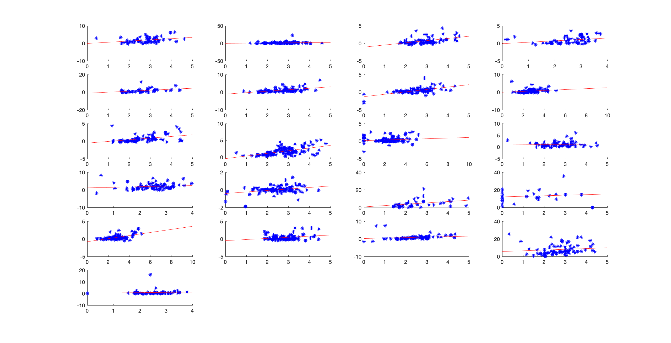
Note: The figures show positive correlations between quality preferences and difference in loss from trade barrier between the model in this paper and Melitz and Ottaviano for sectors: HS 2, HS 3, HS 4, HS 7, HS 8, HS 9, HS 11, HS 15, HS 16, HS 17, HS 23, HS 24, HS 30, HS 35, HS 36, HS 37, HS 38, HS 39, HS 40, HS 42, HS 51

Country Country Country Country ABW 0 DMA 0 BOL -92.825249 GTM -142.23793 AFG 0 DNK -114.35749 BRA -88.041534 GUM 0 AGO -5.9250102 DOM -290.53134 BRB 0 GUY 0 AIA 0 DZA -211.93385 BRN -105.61481 HKG 0 ALB 0 ECU -150.62788 BTN -30.520798 HND -71.087296 AND 0 EGY -139.12598 CAF -6.0313959 HRV -35.601143 ARE 110.83006 ERI 0 CAN -134.60129 HTI 10.083085 ARG -172.65367 ESP -3.0844131 CCK 0 HUN -71.353348 ARM -83.855202 EST -137.4808 CHE -221.01123 IDN -61.682568 ASM 0 ETH -14.915351 CHL 148.51651 IND -79.18856 ATF 0 FIN -139.43924 CHN -18.930056 IOT 0 ATG 0 FJI -1.2493064 CIV -566.53101 IRL -159.63408 AUS -85.625969 FLK 0 CMR 20.903 IRN 125.87421 AUT -35.475746 FRA -48.415028 COG 9.3548021 IRQ -94.298141 AZE -88.898872 FSM 0 COK 0 ISL -217.56667 BDI 197.47388 GAB -317.1246 COL -32.865913 ISR -117.73706 BEL 4.9142151 GBR -89.882896 COM 0 ITA -4.3799672 BEN 340.07468 GEO -77.644836 CPV 0 JAM -181.83876 BFA -499.91898 GHA 313.25208 CRI -150.97874 JOR -117.16895 BGD -52.478401 GIB 0 CUB 0 JPN -34.355942 BGR -193.67613 GIN -221.29001 CXR 0 KAZ -3.359056 BHR 0 GMB -127.25304 CYM 0 KEN 114.01509 BHS -313.15955 GNB 425.91129 CYP -286.89645 KGZ -32.405098 BIH -70.668152 GNQ 164.41464 CZE -132.38187 KHM -155.89485 BLR 9.4817276 GRC -42.363346 DEU -97.001007 KIR 0 BLZ -127.64666 GRD 0 DJI -76.750755 KNA 0 BMU 0 GRL 0 Note: This table summarizes the changes in endogenous cutoffs following an increase in preference for quality
Country Country Country Country KOR -35.787136 QAT -219.32658 MYS -158.87752 TKM -52.555267 KWT -460.9559 ROM 0 NCL 0 TMP 0 LAO -436.81769 RUS -98.661285 NER -230.2971 TON 0 LBN 20.976509 RWA -396.1434 NFK 0 TTO -104.69793 LBR 292.86221 SAU -45.471489 NGA -42.240189 TUN -165.00168 LBY 0 SEN -349.76016 NIC 74.577103 TUR -73.441292 LCA 0 SGP 0 NIU 0 TUV 0 LKA -184.27283 SHN 0 NLD -138.3261 TWN -55.560108 LTU -159.97792 SLB 0 NOR -83.566177 TZA -234.38101 LVA -20.440449 SLE 194.28214 NPL -314.22827 UGA -58.329792 MAC 0 SLV -65.059845 NRU 0 UKR -150.4944 MAR -100.28398 SMR 0 NZL -180.14423 URY -185.035 MDA -37.104824 SOM 0 OMN -0.6131459 USA -83.864113 MDG -21.992657 SPM 0 PAK -30.568909 UZB 110.60154 MDV 0 STP 0 PAL 0 VCT 0 MEX -26.129211 SUR -325.828 PAN -197.16428 VEN -17.546169 MHL 0 SVK -167.24568 PCN 0 VGB 0 MLI 7.2255492 SVN -107.09841 PER -114.9763 VNM -68.709572 MLT 0 SWE -112.68818 PHL -77.56852 VUT 0 MMR -69.190582 SYC 0 PLW 0 WLF 0 MNG -217.73524 SYR -77.680817 PNG 0 WSM 0 MNP 0 TCA 0 POL -64.078629 YEM -515.06506 MOZ -138.54242 TCD 105.06513 PRK 0 ZAF -143.84947 MRT 179.3062 TGO 301.63589 PRT -181.69063 ZAR 0 MSR 0 THA -39.003437 PRY -254.91846 ZMB -184.53088 MUS 0 TJK -232.86932 PYF 0 ZWE 150.78076 MWI 37.507915 TKL 0 Note: This table summarizes the changes in endogenous cutoffs following an increase in preference for quality

| Dependent Variable: | Changes in Cost Cutoff | ||
|---|---|---|---|
| (1) | (2) | (3) | |
| (log) Population | -6.188** | -8.510*** | -8.929*** |
| (3.139) | (2.044) | (3.299) | |
| Initial Preference | -0.795 | -0.634 | |
| (0.606) | (0.700) | ||
| (log) GDP per capita | -13.617 | ||
| (9.317) | |||
| Number of Observations | 168 | 168 | 160 |
| Notes: *** p < 0.01, ** p < 0.05, * p < 0.1. Robust standard errors are in parentheses. The dependent variable in specifications (1)-(3) is the level of aggregate cutoff change at the country-level. Country-level control variables are the initial preferences for quality and (log) GDP per capita. | |||