Predicting the occurrence of Braess paradox in the synchronization threshold of coupled oscillator systems
Abstract
We study Braess-type paradoxes in coupled oscillator networks where the addition of an edge to the network leads to an increase in the critical coupling required for the existence of a stable phase-locked synchronized solution. By introducing a continuous edge-weight parameter and constructing an augmented system that allows application of the Implicit Function Theorem, we derive an explicit first-order formula for the sensitivity of the critical coupling, , to small changes in the network structure. This formula reveals that an edge is locally Braess if the ordering of the oscillators being coupled is opposite the ordering of their components in the critical eigenvector at the saddle-node bifurcation, providing a simple criterion for Braess paradox to occur. We then employ this local approximation as a predictor for the occurrence of Braess paradox when the edge is fully incorporated in the network. This prediction is tested numerically in several classes of random networks, demonstrating both high predictive fidelity and the nonlinear limitations of the local approximation. We also examine several explicit examples, highlighting possible motifs by which Braess-type paradoxes occur. Together, these results establish a predictive framework for understanding how incremental changes in network topology can produce counterintuitive synchronization outcomes.
In oscillator networks described by the Kuramoto model, adding a single new edge can hinder synchronization rather than promote it, with consequences ranging from power grid stability to biological rhythms. This is often called a Braess-type paradox in reference to the well-known fact that adding a new road to a transportation network can sometimes decrease the efficiency of traffic flow. We study this phenomenon in the Kuramoto model and derive an analytical predictor, rooted in the Implicit Function Theorem, that classifies any candidate edge as beneficial or Braess directly from the geometry of the current synchronous state. The result is a fast, mathematically grounded tool for understanding how local structural changes drive global, and sometimes counterintuitive, network behavior.
I Introduction
Braess paradox refers to the counterintuitive phenomenon in which adding an edge to a network can degrade its overall performance. Originally identified in transportation networks Braess (1968), where the addition of a road can paradoxically increase the total travel time of all drivers, the effect was later shown to be widespread in a broad class of networked systems Steinberg and Zangwill (1983). The phenomenon arises not from poor design, but from rational individual behavior that, in aggregate, leads to suboptimal global outcomes, a hallmark of the tension between local and global optimization in complex networks.
This counterintuitive behavior extends beyond transportation to oscillatory networks, where the relevant measure of performance is synchronization rather than travel time. Power grids are a particularly consequential setting for this phenomenon: generators and consumers are represented as nodes with oscillatory dynamics, and the stable operation of the grid depends on maintaining phase-locked synchronization across the network Witthaut and Timme (2012). The loss of synchronization in such systems can trigger cascading failures, making the question of how network topology shapes synchronizability not merely of theoretical interest, but of direct practical importance.
We study the Kuramoto modelKuramoto (1984), a canonical framework for studying synchronization in coupled oscillator systems. In this model, each node represents an oscillator whose phase evolves according to
| (1) |
where is the natural frequency of the th oscillator and is the coupling constant. Interactions between oscillators are described by the adjacency matrix associated with a connected, undirected graph . Each node in the graph is identified with an integer and edges are represented uniquely by ordered pairs with . The adjacency matrix therefore satisfies with if and only if . We adopt the convention to label nodes in the graph in the order of increasing natural frequency. That is, we order nodes in the graph so that implies . By potentially transforming to a rotating frame, we may assume .
The evolution of oscillators in the Kuramoto model (1) is subject to two competing influences. First, each oscillator has its own individual natural frequency, which tends to separate oscillators. At the same time, the nonlinear coupling promotes oscillators to match each other’s phases. The competition between these two effects plays out as follows. When , the oscillators move freely, and each oscillator rotates at nearly constant angular rate equal to its natural frequency. Conversely, when , the nonlinear terms dominate, and there exists a stable steady state solution where all phases are approximately equal. These two regimes are separated by a critical coupling constant , at which this steady state solution disappears through a saddle-node bifurcation. The study of this critical coupling constant and its dependence on the set of natural frequencies and the network of interactions has been an immense field of research over the previous decades Acebrón et al. (2005); Dörfler and Bullo (2011); Rodrigues et al. (2016).
We are concerned with the following problem. Suppose that an edge is added to a network. This leads to additional synchrony-enhancing terms appearing on the right-hand side of (1). It is natural to expect that the addition of these terms should serve to decrease the critical coupling required for synchronization. Braess paradox refers to situations where the opposite occurs, meaning the critical coupling increases instead. The purpose of this article is to study what properties of the steady state solution and the network of interactions would facilitate such a behavior.
We now make some of these ideas precise. The central object of study is the phase-locked (or steady) state, in which all oscillators rotate at a common frequency, and their phase differences remain constant in time. Such states are solutions to the algebraic system
which we write compactly as . Phase-locked states do not exist for arbitrarily small coupling; synchronization emerges only when is sufficiently large to overcome the heterogeneity in natural frequencies. When multiple stable phase-locked states exist, we are interested in the one exhibiting the highest degree of synchrony, as measured by the order parameter
| (2) |
The order parameter quantifies global phase coherence: corresponds to perfect synchronization and to complete incoherence. As we said previously, for , one can show that there exists a stable synchronous state with for all oscillators. This stable state can be continued in the parameter until a bifurcation occurs. This bifurcation is generically a saddle-node, and we define the critical coupling constant as the value of at which this branch of synchronous solutions undergoes a saddle-node bifurcation. We note that other stable synchronous solutions may co-exist with the branch considered here; see the twisted state solutions of Wiley, Strogatz and GirvanWiley et al. (2006) for example. However, these alternate steady states typically have a lower degree of synchrony as measured by the order parameter .

Braess paradox in oscillator networks is generally referred to as a decrease in the level of synchronization in a system after the incorporation of additional coupling terms. Witthaut and Timme Witthaut and Timme (2012) first demonstrated this phenomenon in power grid models, showing that adding edges can destabilize phase-locked states and reduce synchronization, and establishing the presence of Braess paradox through systematic examination of how individual edge additions alter the critical coupling required for stable operation. Subsequent research in this area has focused on various measures of synchronization. Specifically, upon adding or strengthening an edge in the network, one could view Braess-type phenomena as being associated with i) lower degree of synchrony as measured by , ii) larger loads occurring over individual edges in the network, or iii) a decrease in the stability of a phase-locked solution as measured by the value of the least stable eigenvalue appearing in the linearization near the steady state. Arola-Fernandez, Skardal, and ArenasArola-Fernandez et al. (2021) studied how edge additions could lead to a lower degree of synchrony as measured by . They expressed the synchronized state through the Laplacian pseudo-inverse, enabling a geometric analysis of how network structure shapes phase configurations. Manik, Witthaut, and Timme Manik et al. (2017, 2022) analyzed how infinitesimal perturbations in edge strength alter global flow patterns in supply and transport networks, providing a framework for identifying edges whose strengthening can induce Braess-type behavior through an overloading of certain edges. Coletta and JacquodColetta and Jacquod (2016) studied how edge addition can lead to a decrease in the stability of a phase-locked solution, as measured by the value of the least stable eigenvalue appearing in the linearization near the steady state, with a primary focus on chain networks. While not phrased explicitly in terms of Braess paradoxes, work by Motter, Zhou and KurthsMotter et al. (2005) showed how heterogeneity in network connections could decrease synchronization. Taylor, Skardal and SunTaylor et al. (2016) study optimization of synchronization through the derivation of a synchrony alignment function meant to quantify the interplay between network structure and individual frequencies. Together, these works make clear that the relationship between the network’s connectivity and synchronizability is subtle and non-monotone.

In this work, we adopt a slightly different approach and characterize Braess paradox in terms of how the critical coupling changes under a small structural perturbation of the network, specifically, the addition of a single new edge; see Figure 2 for an example potential impact. Our main result (Theorem 1 in Section II) is a derivation of an analytical formula, based on the Implicit Function Theorem, that predicts the sign of this change. Our framework applies to general oscillator networks and allows one to predict whether a candidate edge is Braess (edge addition raises , hindering synchronization) or non-Braess (edge addition lowers , facilitating synchronization) without requiring full recomputation of the phase-locked state for every edge under consideration. The primary insight gained from our analysis is that Braess edges arise primarily when they couple oscillators whose ordering of phases is opposite the ordering of the respective entries in the critical eigenvector at the saddle-node bifurcation. We analyze the accuracy of this classifier, including cases of false positives and false negatives, and identify network archetypes in which behavior type arises. A representative example of the phenomena studied in this work is shown in Figure 1, where candidate edges on an Erdös Rényi random network are classified according to their effect on the critical coupling ; our predictor correctly identifies most edges, though occasional misclassifications (false positives in orange, false negatives in purple) reveal the boundaries of the linear approximation. A secondary result (Theorem 2 in Section II) computes how the order parameter varies with small changes in the network. This result requires a full understanding of the spectrum of the steady state solution. However, we apply it in some degenerate cases and show that it recovers the condition derived in Arola-Fernandez, Skardal, and ArenasArola-Fernandez et al. (2021) in the limit as .
The remainder of this paper is organized as follows. In Section II, we introduce the mathematical framework and state the main results. Specifically, we define the augmented system that encodes the addition of a new edge with weight , and formally state Theorem 1, which provides an explicit formula for via the Implicit Function Theorem, yielding a computable criterion for predicting whether a candidate edge is Braess. We complement this with Theorem 2, which characterizes how the order parameter responds to the edge addition near a stable synchronous state, and we discuss the geometric interpretation of both results. In Section III, we test the validity of the analytical prediction of Theorem 1 against numerical simulations on planar random geometric graphs of varying scale, examining the classifier performance, including rates of true and false positives and negatives, and identifying the role of coupling oscillators whose phase differences exceed as a source of prediction error. In Section IV, we analyze several network motifs in which Braess behavior can be understood explicitly, providing structural intuition for the conditions under which the paradox arises. Section V concludes with a discussion of the results and directions for future work. Proofs of Theorems 1 and 2 are collected in Appendices A and B, respectively.
II Main Theorem: Braess edge prediction via Implicit Function Theorem
Our goal is to calculate how our critical coupling changes upon adding a new edge of weight between two nodes and . So, we define a parameter where represents the lack of an edge between node and , while represents the full addition of the edge. Considering as a function of , we want to differentiate and compute . We first redefine our steady state equation to incorporate the new addition of an edge.
Definition 1.
Let such that
| (3) |
where ,
and
We specify for uniqueness that , and represents the -th standard basis vector. We define the steady state equation when .
Suppose that when , there exists a steady state solution that undergoes a saddle-node bifurcation at . At this bifurcation, the Jacobian, has a double zero eigenvalue. One eigenvector is the constant vector , which always lies in the kernel of the Jacobian since it has a row sum of zero. We denote the second eigenvector , which is orthogonal to . We can then derive an explicit first-order formula for the critical coupling strength, , as the edge weight is increased incrementally from . Our main result is the following.
Theorem 1.
Suppose that when , there exists such that and its Jacobian, , has a null vector satisfying , , and
Then, for near , there exists smooth functions , , such that
and with for all near . Moreover, if then
| (4) |
Proof.
The first step of the proof is to show persistence of the saddle-node bifurcation to synchrony, assumed to hold when and . Towards that end, we consider the following augmented system:
| (5) |
We will show that there exists a solution to for all sufficiently small. This solution will be the continued saddle-node bifurcation to synchrony. The first equations in (5) enforce a steady state solution to (1). The following equations enforce the existence of a kernel element to the linearization. The last three conditions normalize this kernel element to be a unit vector, enforce that this vector is orthogonal to the kernel element , while the final phase condition removes the phase invariance in (1).
The existence of a curve with , , , for which follows from a Liapunov-Schmidt reduction; see Appendix A for details.
Theorem 1 establishes a criterion dictating whether the critical constant increases or decreases when the weight of edge is increased by some small amount. Since one expects additional connectivity to reduce the synchronization threshold, an increase in is seen as counterintuitive and categorizes such edges as Braess edges in the following manner.
Definition 2.
The edge is a Braess edge if . The edge is locally Braess if .
In the context of (1), the edge is a Braess edge if the critical coupling is larger when the edge is included in the adjacency matrix . Theorem 1 provides a local description of whether is increasing or decreasing for small edge weight . This local behavior can be used as a prediction for the critical coupling when and the edge is fully incorporated in the network. We formulate this as the following prediction.
Prediction 1.
The edge is a Braess edge if .
We use the phrasing prediction as opposed to conjecture because we do not expect this to hold universally for all edges. Numerical investigations of the accuracy of this prediction in some sample networks are presented in Section III. Here, one can consider the critical coupling constant as a function of the added node weight . A locally Braess edge will necessarily satisfy that the graph of will be locally increasing near . Theorem 1 further denotes the only two generic ways in which this graph can lose non-monotonicity: either the phases of the coupled oscillators will match for some value of or the respective values in the critical eigenvector will. Interestingly, our numerics reveal that it is typically the case that edges which are locally Braess but not Braess (false positive predictions) will see that the phases of the respective oscillators to swap at some intermediate value of , whereas edges which are Braess but not locally Braess (false negatives) will see that the respective entries in the critical eigenvector will swap. See examples in Section III and Section IV for more details.
Suppose that the phase difference between the two oscillators and is less than in magnitude. Theorem 1 gives a simple criterion to identify whether the edge is locally Braess: if the oscillator phases’ ordering is opposite to that of the respective elements’ ordering of the entries in the (normalized) critical eigenvector, then the edge is locally Braess. To make this precise, we specify a unique phase for each oscillator as the unique phase (subject to the phase condition ) for which
One might also be interested in the behavior of the order parameter when a new edge is added to the network. The following results give the derivative of as a function of the parameter .
Theorem 2.
Suppose that there exists a stable synchronous steady state solution . Denote the eigenvalues of the linearization by with the assumption that with corresponding orthonormal eigenvectors . Then there exists a steady state solution and the order parameter is locally a smooth function of whose derivative satisfies:
| (7) |
where
| (8) |
and
| (9) |
Proof.
The proof follows by fixing the rotational symmetry and applying the Implicit Function Theorem and is presented in Appendix B. ∎
Theorem 1 and Theorem 2 generalize immediately to Kuramoto models on weighted graphs described by the system of equations:
| (10) |
The only difference between (10) and (1) is that the matrix can prescribe arbitrary positive weights to edges as opposed to the unitary weights prescribed by the non-zero entries of .
Remark 1.
In the limit as from above, we have that ; see the statement of Theorem 2. Observe that in this limit, the dominant contribution guiding whether the order parameter is increasing or decreasing is exactly the product of and the difference .
III Numerical investigations on random networks
We tested the prediction of Theorem 1 on randomly generated oscillator networks. For a missing edge , define
so that is the original network and is the network after the full edge has been added. In the numerical computations, an edge was treated as Braess when
Here denotes the numerically estimated synchronization threshold described below. The local prediction was obtained from the sign of the derivative in Theorem 1,
Thus predicts a Braess edge and predicts a non-Braess edge. In the implementation, the critical eigenvector is always oriented so that .
Network ensembles.
We considered two different random graph models. For Erdős–Rényi graphs, we repeatedly sampled with until the graph was connected. For planar random geometric graphs, node positions were sampled independently in , and two nodes were connected whenever their Euclidean distance was at most ; this process was also repeated until the graph was connected. Natural frequencies were sampled independently from Unif[-1,1] and then shifted so that they had a mean of zero. The phase gauge was fixed by setting .
Computing the numerical threshold.
The code does not compute an exact saddle-node bifurcation point. Instead, it estimates using numerical continuation. For each network, the solver begins at and employs secant continuation to follow this branch of stable phase-locked solutions until stability is lost in a saddle-node bifurcation and the critical coupling constant is identified as the minimal constant along this branch of solutions.
Filtering and evaluation.
Our numerical investigations computed for ensembles of networks of Erdös-Rényi and random geometric graph types. In each case, we compute the base critical value and the value of from Theorem 1. To limit computational time, we only consider edges for which the predicted relative deviation in the critical coupling constant exceeds .
Aggregated data over 20 different random geometric networks with nodes is shown in Figure 3. Edges are classified as true/false-positive/negative depending on whether our prediction based upon is accurate and if it predicts the edge to be Braess or not. We report a relatively high number of false positive cases, which we attribute to two sources. First, we see a significant number of false positive cases relating to the coupling of oscillators with a variety of frequencies, nearly between and . Closer investigation reveals that most of these occurrences involve edges that are only weakly locally Braess in the sense that the predicted relative change in the critical coupling constant is small, i.e., close to the cutoff used in the numerical process. We therefore refine our prediction to only consider edges with a predicted relative deviation exceeding . This data is reported in Figure 4.

The data in Figure 4 shows that restricting consideration to only those edges with relative change exceeding improves our prediction for moderate phase differences, but false positive outcomes persist for edges that connect oscillators with phase differences exceeding in magnitude. The reason for this will be studied in more detail in some example networks in Section IV. A scatter plot of predicted versus observed changes in the critical coupling constants is also provided in Figure 4. We note somewhat linear behavior associated with the data near the origin. As expected, there are many more edges whose addition contributes a greater degree of synchronization (true negative cases), and the addition of some edges can lead to quite large decreases in the critical coupling values.


Additional numerical investigations in support of being a useful predictor for the occurrence of Braess paradox are presented in Figures 5-7. We present outcomes for twenty realizations each of random geometric graphs with and nodes and Erdös-Rényi random graphs with and nodes. In each trial, we consider the addition of all edges for which the criterion in Theorem 1 predicts a relative change in the critical coupling exceeding , positive or negative. Overall, we find that our predictor performs strongly whenever the phase difference between coupled oscillators is less than in magnitude. For the random geometric graphs in particular, these results require filtering out edges whose predicted relative change falls below a more stringent threshold. To state some specific results, consider the example of random geometric graphs presented in Figure 4. When restricting our consideration to potential edges for which i) a relative change in of magnitude of or greater is predicted, and ii) coupling oscillators with an absolute phase difference less than , we find true negative cases, true positive cases, false negative cases, and false positive cases. Thus, our predictor is correct in over of these cases. Similar levels of success are obtained on larger networks and for Erdös-Rényi networks.


False positive and false negative edges
Theorem 1 provides some insight as to the mechanisms that might contribute to inaccuracies in our predictions. Specifically, under generic assumptions, Theorem 1 identifies two distinct possibilities by which may not be monotone. Suppose that indicating that is a locally Braess edge. If this edge fails to be Braess, then necessarily, there must exist an for which . This can only occur if either i) the phases of the oscillators satisfy for some , ii) the respective entries in the critical eigenvector match, i.e., , or iii) a degeneracy occurs in which either the nontrivial critical eigenvector is no longer unique or remains unique, but the non-degeneracy condition fails. We observe that false positive cases where the phase difference between oscillators exceeds typically exhibit a case i) where increased coupling eventually draws the oscillators closer, and the derivative of changes sign. We also note that most of the false negative cases that we observe arise due to ii) where the entries in the critical eigenvector coincide for some non-zero value of the coupling weight .


Representative examples.
We provide four specific examples from our investigations. Figure 8 and Figure 11 show Erdös Rényi random graphs with two qualitatively different outcomes. Figure 8 represents a situation where our results work well. The network has two differentiated nodes whose phases are distinct from the bulk of the network. Added edges can either connect nodes within the bulk of the network or connect the differentiated nodes to nodes in the bulk. The second case (bulk-to-isolated node connections) leads to large decreases in the critical coupling constant, although due to nonlinear effects, these decreases are limited in their total effect. For nodes connecting two nodes in the bulk, our predictions work quite well with strongly linear behavior between predicted and observed deviations in the critical coupling. Figure 11 shows a slightly different situation where there exists a single differentiated node that is connected to a single node in the bulk. At the critical coupling constant, the critical eigenvector is piecewise constant, so additional edges that further couple the bulk to itself will have due to their critical eigenvector components being equal. This situation is explained in more detail in the case of simple chain networks below.
As we emphasized previously, our predictor is based upon the derivative , and nonlinear effects could lead to false predictions. We show two examples of the graphs showing how they may depend on the parameter . Figures 9–10 show a representative true positive Braess edge in the case of a random geometric network. The highlighted added edge is predicted to be Braess by the sign of , and the full edge addition increases the numerically estimated threshold. The sampled curve agrees with the initial direction predicted by the derivative. Figures 12–13 show a representative false positive example. The local derivative predicts Braess behavior, but the full edge addition lowers the numerically estimated critical coupling, illustrating the nonlinear limitation of the first-order predictor.


IV Motifs and Examples
In previous sections, we derived an explicit analytical criterion for the effect of a newly added edge on the critical coupling constant, and leveraged this local prediction to assess the impact of fully incorporating the edge into the network. In this section, we consider several sample networks with simpler network topologies to illustrate various aspects of the theory. We start with simple chain networks, where explicit computations are possible and to illustrate why we limit our classifier to only consider edges of coupling oscillators with phase differences less than . We consider two network topologies from previous studies of Braess phenomena in coupled oscillator networks to compare and contrast our approach with prior work. Finally, we briefly comment on the applicability of our results to large dense networks using some continuum limit analysis, making use of graphons.
Example: Chain Network
The simplest way in which the linearization can gain a second zero eigenvalue is if there exists an edge in the graph such that if the edge is removed, the network becomes disconnected. The most basic setting in which this arises is a chain network. Slightly deviating from our notation thus far, we order nodes so that for all and let be the natural frequency of oscillator , so that the may no longer be increasing. We still assume that is mean zero, and we fix the phase condition . Let
Then there exists a steady state solution of the form
provided that for all . We then obtain . When there exists an edge for which the phase difference . The Jacobian evaluated at this steady state is therefore block diagonal, and the critical eigenvector is piece-wise constant, taking the form:
Without loss of generality, we suppose . Now add the edge to the network, for some . Theorem 1 then implies that – supposing that the phase difference between oscillators is less than in magnitude – this edge will be locally Braess if and only if , and .
Now consider a 6 node chain with , see Figure 14. Then and we have . The critical eigenvector is a scalar multiple of the frequency vector: . Theorem 1 then implies that if and only if . Assuming then that we find
where we have used , and . We then obtain the following: if the phase difference between the newly coupled oscillators is less than , then , the edge addition promotes synchrony, and is not locally Braess. However, if the phase difference is larger (between and ), then the edge is locally Braess and, at least for small , the addition of the new edge will require a larger coupling constant to achieve synchrony.
The reason for this is simple: when , the critical coupling constant occurs because the phase difference between oscillators 3 and 4 equals . Coupling between oscillators 1 and 6 will draw these oscillators closer together, but because the phase differences are greater than , this has a secondary effect of increasing phase differences between the remaining oscillators, contrary to what is required to establish synchrony; see Figure 14. Therefore, a larger coupling strength is required to maintain the phase-locked pattern. It is interesting that in many of the examples that we have considered, these locally Braess edges are not often Braess when the edge is fully incorporated in the network.


Going beyond chain networks, a similar line of analysis may be applied to networks where the critical coupling is determined by the existence of an edge connecting two oscillators with a phase difference of . If removing this edge leads to a disconnected graph, then the analysis of the chain network can be immediately extended. To do so, consider the two subgraphs after the removal of this edge. Locally Braess edges are only possible for new edges spanning these two components. We illustrate one such situation arising in an Erdös Rényi network in Figure 11.
Example: Erdös Rényi random graphs in the large node limit
Another perspective can be gained by passing to a continuum limit where the discrete adjacency matrix is replaced by a continuous function – referred to as a graphonBorgs et al. (2008); Bramburger et al. (2025); Medvedev (2019); Lovász (2012) – whereby the discrete system (1) is approximated by the nonlocal equation:
| (11) |
where is a continuous function describing the frequency of the oscillator at location , and describes the strength of the connection between nodes at latent position and . We assume that is non-decreasing with and odd with respect to so that it has a mean of zero. The existence of a phase-locked state for various distribution functions was studied by Ermentrout Ermentrout (1985) in the case of all-to-all coupling, where , while extensions to Erdös-Rényi random graphs with were recently considered in Bramburger and HolzerBramburger and Holzer (2025). For bimodal frequency distributions, the transition to synchrony in (12) occurs due to a saddle-node bifurcation at a critical coupling parameter . To study how changes in the graph impact the onset of synchrony, we consider the equation
| (12) |
where describes the addition of edges to the graph in accordance with the discrete setting in (3). The following generalization of condition (4) holds here:
Suppose for the moment that is supported near the pair of points and with . Then, normalizing so that the denominator is positive, we find
for some . Then, since is monotone increasing with range contained in the interval , we find that a Braess phenomenon can occur only if there exist points such that and . In other words, Braess phenomenon is possible if the critical eigenfunction is non-monotone. While explicit representations of are not often available, for all the distribution functions that we checked, the critical eigenfunction is monotone. This suggests that there is no systematic way to add edges to an Erdös-Rényi graph which will lead to shifts in that remain order one in the limit as the number of nodes in the random graph tends to infinity. In fact, any graphon perturbation will tend to generically decrease the critical coupling threshold, especially if it enhances connections between nodes near and .
Example: simple ring network with symmetry
When the network under consideration has some symmetry, it may be the case that the Jacobian has a kernel of dimension greater than two, and Theorem 1 will not apply. In these situations, Theorem 2 remains applicable. We illustrate this in the following example, studied also in Section IV.D (Figure 2) of Manik, Witthaut and Timme Manik et al. (2017). We deviate somewhat from the previous examples and consider here changes in graph weights as in (10) rather than new edge addition. The example is interesting in that it provides an example of a network modification which both shifts the value higherManik et al. (2017) while also increasing the measure of the order parameter according to Theorem 2.
Consider a 4-node ring network ---- where nodes and have natural frequency and nodes and have natural frequency , so that . The network has the following steady state solution (imposing the phase condition ):
where , valid for any . The critical coupling constant is therefore . The Jacobian takes the form:
since every edge of the ring crosses the same phase gap , contributing to each off-diagonal entry.
At , we have , hence , so the Jacobian vanishes identically. The kernel of is therefore all of , which is four-dimensional rather than the two-dimensional kernel required by Theorem 1. Consequently Theorem 1 does not apply at this bifurcation point, and we instead apply Theorem 2 for , where the steady state is stable and all eigenvalues are strictly negative.
The Jacobian is times the 4-cycle Laplacian, whose eigenvalues are , giving the ordered eigenvalues
with corresponding orthonormal eigenvectors and
Note that is a degenerate eigenvalue, arising because every edge of the ring crosses the same phase gap , so the Jacobian has uniform off-diagonal entries. Any linear combination of and is also a valid eigenvector for this eigenvalue; the choice above gives a convenient orthonormal basis.
The base network is the 4-cycle ---- with all entries of the adjacency matrix equal to , so that each edge carries effective coupling strength . We consider the effect of increasing the weight of the existing edge by perturbing its weight from to , applying Theorem 2. Since , we compute
and applying at each node:
giving
Computing the projections :
For the edge , we compute :
Since , only contributes:
Substituting into (7) with and :
Since implies , we have and , so . This means that, for fixed , the order parameter is locally increasing with respect to the edge weight perturbation at ; equivalently, increasing the weight of the edge from its nominal value increases the degree of synchronization.
Remark 3.
We note that the two candidate new edges, the diagonals and , both connect nodes having equal equilibrium phases, so for both, giving trivially.
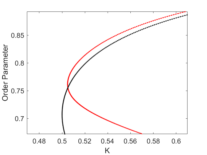
In Manik et al.Manik et al. (2017) it is observed that the perturbation to the weights leads to an increase in the critical coupling constant and therefore the edge is locally Braess. However, our application of Theorem 2 shows that, for any , the order parameter also increases describing an increase in synchronization as measured by the order parameter ; see Figure 15. The two criteria thus operate on different aspects of the synchronization landscape.
V Discussion
In this work, we have studied the Braess paradox in Kuramoto oscillator networks through the lens of the Implicit Function Theorem. Our main result, Theorem 1, provides an analytical formula for the derivative that predicts whether adding a new edge to a network will raise or lower the critical coupling constant , and thus whether the addition hinders or facilitates synchronization. The formula (4) is computationally inexpensive to evaluate: it requires only the phase-locked state , the critical eigenvector , and the natural frequencies of the base network, all of which are computed once and reused to screen every candidate edge. This stands in contrast to brute-force approaches that require a full numerical continuation for each candidate edge, which is computationally prohibitive for large networks.
The formula in Theorem 1 admits a transparent geometric interpretation. The sign of is determined by the interplay between two quantities: the phase difference between the two oscillators to be connected, and the difference in the corresponding entries of the critical eigenvector. Specifically, the edge is predicted to be Braess when the phase ordering of the oscillators is opposite to the ordering of their critical eigenvector components, provided the phase difference satisfies . This dichotomy offers an intuitive explanation for the Braess phenomenon in oscillator networks: adding an edge between oscillators whose relative phases are misaligned with the critical mode of the network can inadvertently stiffen the system and raise the synchronization threshold.
This geometric picture also clarifies when the predictor is expected to fail. When the phase difference exceeds , then the addition of coupling between these two oscillators will have the downstream effect of increasing phase differences between the remaining oscillators, contrary to what is required for synchronization. This leads to a larger coupling required for small coupling strengths, but interestingly, it seems to be the case that larger coupling strengths realign the oscillator phases so that the phase difference between oscillators spanning the coupled edge drops below .
Our numerical investigations, presented in Section III, reveal that the predictor performs well across a range of network types, correctly classifying the majority of candidate edges as Braess or non-Braess. Two distinct failure modes were identified. False positives, edges predicted to be Braess that are observed to be non-Braess, arise most frequently when the phase difference between the two oscillators is near . False negatives, edges predicted to be non-Braess that are observed to be Braess, are rarer and tend to arise when the function is non-monotone and the initial slope underestimates the destabilizing effect of the new edge at finite weight .
The plots presented in Section III further illuminate the limitations of the local prediction. While correctly predicts the initial direction of change for most edges, the function can be non-monotone on : an edge that initially raises may ultimately lower it, or vice versa. The chain example in Section IV provides a concrete illustration of this non-monotone behavior, where the interplay between local phase differences and global network topology produce a non-trivial dependence of on the edge weight .
The motif analysis of Section IV reveals that the Braess phenomenon in oscillator networks is intimately connected to the structure of the critical eigenvector and the geometry of the phase-locked state. In chain networks, Braess edges arise when a new connection bridges two oscillators whose phase difference is large, effectively introducing a competing pathway that disrupts the phase coherence of the existing synchronous state. In ring networks with alternating frequencies, the high degree of symmetry leads to a degenerate critical point at which our theorem’s hypotheses are not satisfied for the full nonlinear system, yet Theorem 2 can still be applied to characterize the behavior of the order parameter near stable synchronous states away from criticality.
The graphon perspective introduced in Section IV points toward a continuum limit in which our discrete formula may be replaced by an integral operator. This limit may allow for analytical predictions of Braess behavior in large random networks without requiring explicit computation of the critical eigenvector, and represents a promising direction for future work. For dense Erdös Rényi networks, we presented an argument that there is no systematic way to add edges that are Braess when the number of nodes is taken to be sufficiently large. We anticipate that other random network models based upon graphons should exist, such that they admit Braess edges in general. One avenue to construct such graphs would be to consider stochastic block model graphons based upon lower-dimensional graphs that exhibit Braess edges.
Of course, several natural extensions of this work suggest themselves. First, the extension to weighted graphs described by (10) is immediate, as noted in Section II, and raises the question of optimal edge weight allocation: given a budget of total edge weight to distribute across a set of candidate edges, how should the weights be chosen to minimize ? Second, the non-monotone behavior of observed in Figure 13 suggests that higher-order corrections to the IFT formula may provide a more accurate global predictor, particularly for edges near the decision boundary. Finally, the extension of our IFT-based classifier to directed and time-varying networks remains an open problem. In directed networks, the Jacobian is no longer symmetric, so the left and right kernels differ and the formula (4) must be modified accordingly. In time-varying networks, the notion of a phase-locked state itself requires reinterpretation. These extensions would broaden the applicability of the Braess paradox classifier to a wider class of real-world networks where directionality and non-stationarity are unavoidable features of the underlying dynamics.
Author Contributions
Author names are listed alphabetically. Justin Arches: Writing – review & editing. Emmanuel Fleurantin: Conceptualization, Formal analysis, Methodology, Supervision, Writing – original draft, Writing – review & editing. Matt Holzer: Conceptualization, Formal analysis, Methodology, Project administration, Supervision, Writing – original draft, Writing – review & editing. Siddhant Sood: Software, Numerical Validation, Visualization, Writing – review & editing. Shakeeb Uddin: Validation, Writing – review & editing.
Data Availability Statement
The data that supports the findings of this study are available from the corresponding author upon reasonable request.
Acknowledgments
M.H. was partially supported by the NSF grant DMS-2406623. The authors would like to thank the Mason Experimental Geometry Lab (MEGL) for providing a collaborative research environment that helped shape the ideas in this work. A special thanks goes out to Abdullah Hatif for his valuable contributions during the Fall 2025 semester, which helped lay the groundwork for this project. Numerical continuation code written by Jason Bramburger in a prior collaborationBramburger and Holzer (2025) was adapted to perform some of the numerical simulations conducted.
Author Declarations
The authors have no conflicts to disclose.
Appendix A Proof of Theorem 1
Recall that throughout this section (and the manuscript), we impose . This is necessary for a phase-locked (steady-state) solution to exist, since summing the steady-state equations over all gives .
Remark 4.
From the steady state map in Definition 1, when , the map reduces to
which is the original Kuramoto equation. For general , the - and -components of acquire the additional terms
while all other components are unchanged.
Now fix . The Jacobian of with respect to is
| (13) |
Lemma 1 (Kernel of the Jacobian).
Let be a critical steady state, i.e., and is the smallest coupling for which a steady state exists. Then is a weighted graph Laplacian, every row sums to zero, and
Moreover, there exists a nonzero vector such that .
Proof.
For , the only term in that depends on is , so
For the diagonal, every off-diagonal term depends on , giving
This yields the formula in (13).
Now fix any row . Then
Hence , so and . Finally, the matrix has the form of a weighted graph Laplacian with edge weights . Because is the critical coupling, the Jacobian acquires an additional zero eigenvalue beyond the structural one from above. Thus, there exists a nonzero satisfying , completing the proof.
∎
To apply the Implicit Function Theorem (IFT), we track the critical null vector as the edge weight varies. We encode the steady-state equation, the criticality equation, a normalization, an orthogonality constraint to isolate the non-trivial null vector, and a gauge fix into a single augmented system.
Definition 3.
Augmented System Define by
The five blocks serve distinct purposes:
-
•
: the steady-state equation ( equations).
-
•
: the matrix-vector product tracking the non-trivial null vector of the Jacobian at criticality ( equations).
-
•
: normalization of ( equation).
-
•
: orthogonality of to the trivial Laplacian null vector , isolating the non-trivial critical null vector ( equation).
-
•
: gauge condition fixing the rotational symmetry of the Kuramoto model ( equation).
The free parameter is ; the solve-for variables are .
Remark 5.
At and at the critical point, has a two-dimensional kernel spanned by (trivial, present for all ) and (non-trivial, appearing only at ). The constraint removes the trivial direction, while removes the scaling ambiguity. Together they enforce in the restricted sense needed for IFT.
The partial Jacobian is a matrix given by
| (14) |
where
| (15) |
and
| (16) |
The last identity follows from the fact that is linear in , so that . At the critical point , we have , so the second block of the third column vanishes identically. The domain ( variables) and codomain ( equations) have a two-dimensional mismatch, so IFT cannot be applied directly. We resolve this via an orthogonal projection.
Lemma 2 (Cokernel of ).
The Jacobian , holding fixed, has a two-dimensional left null space (cokernel) spanned by the orthonormal vectors
where .
Proof.
We show and then verify orthonormality.
Now, the first block of is . Since and owing to the anti-symmetry of sine, the components of sum to zero for all :
The first sum is zero since is mean zero. For the second sum, since and is odd, the and terms cancel pairwise, giving zero. For the third sum, , so . Hence identically. Differentiating this identity with respect to gives
The second block of is . Since is a symmetric matrix (the graph is undirected), its row sums equal its column sums. We showed in Lemma 1 that all row sums are zero, so all column sums are also zero, i.e., . Therefore
for all . Differentiating with respect to
gives .
For the orthonormality, note that
since the nonzero entries of and occupy disjoint blocks. Hence is an orthonormal set in the left null space of .
Under the non-degeneracy assumption that these are the only left-null directions (verified numerically for the networks studied here), the cokernel is exactly . ∎
Definition 4 (The Projection ).
Since are orthonormal, define the orthogonal projection onto their orthogonal complement by
The image of is -dimensional and lies inside .
Lemma 3 (Range Condition).
For all , the vector lies in , i.e., for .
Proof.
Both identities were established in the proof of Lemma 2: and , holding for all arguments, not only at solutions. ∎
Corollary 1.
if and only if .
Proof.
Remark 6.
This is the key step that is sometimes called the "range condition" in Lyapunov–Schmidt reduction. The projection kills exactly the cokernel directions, and Corollary 1 ensures that no information is lost by working with instead of itself.
After applying , the first component (index , the -direction, corresponding to the mean of the -block) and the -st component (index , the -direction, corresponding to the mean of the -block) of are identically zero. Dropping these redundant outputs yields a map
so that . By Corollary 1, if and only if . And now we are in a position to apply the IFT.
Lemma 4 (Conditions for IFT).
Let be as above, so . Treat as the free parameter and as the solve-for variables. Suppose:
-
1.
There exists a critical point such that .
-
2.
is continuously differentiable in a neighborhood of .
-
3.
The partial Jacobian is a square matrix (domain and codomain dimensions match with held fixed).
-
4.
is invertible. (This is a genericity condition, verified numerically for the networks studied here)
Then there exist smooth functions , , defined for near such that , , , and for all near .
Conditions (i)–(iv) are precisely the hypotheses of the classical Implicit Function Theorem applied to . The conclusion follows immediately from the standard IFT.
We now have all the ingredients to finalize the proof of Theorem 1. By Lemma 4, there exist smooth functions , , such that for near . By Corollary 1, if and only if , so in particular the first block of gives for all near .
Since and all functions are smooth, we differentiate with respect to and evaluate at . By the chain rule,
| (20) |
We compute each term separately.
For the term : differentiating with respect to gives:
which at equals .
For the term : differentiating with respect to gives
which at equals .
Substituting into (20) at :
| (21) |
Now multiply (21) on the left by :
Since is in the kernel of (this is the second block of , at ), the matrix is symmetric, so its kernel equals its left kernel:
Therefore, the first term vanishes, leaving
By the genericity condition, , we may solve:
Recall that
and at the steady state, when ,
Thus,
and
Now expanding and at , then substituting yields
This completes the proof.
Appendix B Proof of Theorem 2
Proof.
Suppressing the dependence on , we seek zeros of the following function subject to the phase condition . Let be the orthogonal projection defined via for each eigenvector with non-zero eigenvalue . We then define
Note that and is invertible since its kernel and cokernel are trivial. Therefore, the Implicit Function Theorem gives the local existence of a function satisfying .
Recall the definition of the order parameter ; see (2). Noting that we are considering as a function of the edge weight parameter , this can be expressed as
Define and . Differentiating with respect to and evaluating at we find
which simplifies to
where has components .
We have that
Differentiating with respect to and evaluating at yields
Since
we have
and therefore
Recalling the representation
with . Since and we may apply the reduced inverse
acting on the orthogonal complement of . Then
which expands as
Substituting into the expression for and using gives equation (7). ∎
Appendix C Theorem 2 as applied to Erdös-Rényi random graphs
In Arola-Fernandez, Skardal and ArenasArola-Fernandez et al. (2021), a criterion for Braess paradox is derived in the context of random networks and applied to Erdös Rényi random graphs in particular. This criterion applies for large where the following expansion is valid:
where is the degree of the th node. We then write
| (22) |
where with and , and the operator is understood as acting on the range of . Following the approach in Arola-Fernandez et al.Arola-Fernandez et al. (2021), the idea is to approximate
and obtain, utilizing the fact that to obtain
We therefore recover from Theorem 2 the same prediction as in Arola-Fernandez et al.Arola-Fernandez et al. (2021) as the leading order term in the expansion for the derivative of with respect to for large.
References
- The kuramoto model: a simple paradigm for synchronization phenomena. Reviews of modern physics 77 (1), pp. 137–185. Cited by: §I.
- Geometric unfolding of synchronization dynamics on networks. Chaos: An Interdisciplinary Journal of Nonlinear Science 31 (6). Cited by: Appendix C, Appendix C, Appendix C, §I, §I, Remark 2.
- Convergent sequences of dense graphs i: subgraph frequencies, metric properties and testing. Advances in Mathematics 219 (6), pp. 1801–1851. Cited by: §IV.
- Über ein paradoxon aus der verkehrsplanung. Unternehmensforschung 12 (1), pp. 258–268. Cited by: §I.
- Capturing the critical coupling of large random kuramoto networks with graphons. arXiv preprint arXiv:2503.01589. Cited by: §IV, Acknowledgments.
- Persistence of steady states for dynamical systems on large networks. Journal of Nonlinear Science 35 (6), pp. 112. Cited by: §IV.
- Linear stability and the braess paradox in coupled-oscillator networks and electric power grids. Physical Review E 93 (3), pp. 032222. Cited by: §I.
- On the critical coupling for kuramoto oscillators. SIAM Journal on Applied Dynamical Systems 10 (3), pp. 1070–1099. Cited by: §I.
- Synchronization in a pool of mutually coupled oscillators with random frequencies. Journal of Mathematical Biology 22 (1), pp. 1–9. Cited by: §IV.
- Chemical turbulence. In Chemical oscillations, waves, and turbulence, pp. 111–140. Cited by: §I.
- Large networks and graph limits. Vol. 60, American Mathematical Soc.. Cited by: §IV.
- Cycle flows and multistability in oscillatory networks. Chaos: An Interdisciplinary Journal of Nonlinear Science 27 (8). Cited by: §I, §IV, §IV.
- Predicting braess’ paradox in supply and transport networks. arXiv preprint arXiv:2205.14685. Cited by: §I.
- The continuum limit of the kuramoto model on sparse random graphs. Communications in Mathematical Sciences 17 (4), pp. 883–898. Cited by: §IV.
- Enhancing complex-network synchronization. EPL (Europhysics Letters) 69 (3), pp. 334–340. Cited by: §I.
- The kuramoto model in complex networks. Physics Reports 610, pp. 1–98. Cited by: §I.
- The prevalence of braess’ paradox. Transportation science 17 (3), pp. 301–318. Cited by: §I.
- Synchronization of heterogeneous oscillators under network modifications: perturbation and optimization of the synchrony alignment function. SIAM journal on applied mathematics 76 (5), pp. 1984–2008. Cited by: §I.
- The size of the sync basin. Chaos: An Interdisciplinary Journal of Nonlinear Science 16 (1). Cited by: §I.
- Braess’s paradox in oscillator networks, desynchronization and power outage. New journal of physics 14 (8), pp. 083036. Cited by: §I, §I.