Phase-Drift Limits and Adaptive Quadrature Readout
in Programmable Photonic Processors
Abstract
Phase fluctuations between optical inputs limit programmable photonic processors because their output powers depend on coherent interference. We study the phase-drift penalty that arises when sine and cosine quadratures are measured sequentially rather than simultaneously. The analysis is motivated by phase-drift measurements from an eight-mode programmable photonic processor, in which two equal-power inputs were mapped to four output powers and 35 free-running recordings of 300 s were acquired at approximately 125 samples per second per channel. These recordings provide an empirical route for estimating the phase-increment variance associated with a selected reconfiguration interval, while the receiver laws remain independent of a particular drift model.
The estimate is defined at the time of the second measurement. For fixed quadrature order, a detailed perturbation of the exact reconstruction gives
, where is the relative-phase change during reconfiguration. Writing , uniform phase averaging gives the first-order drift mean-square error . A phase-predicted ordering rule measures the locally less informative quadrature first and the more informative quadrature second. Its uniform first-order penalty is , which is 84.9% below the fixed-order value.
We further derive an increment-aware estimator from a local state-space model. Marginalizing the unknown phase increment increases the variance of a stale phase observation by , reducing its Fisher information from to . For ideal balanced Poisson detection, the Fisher information of each quadrature equals its detected signal-photon number. This provides a physical resource interpretation and leads to dimensionless architecture boundaries in the plane of spatial information and phase-increment variance. Exact nonlinear Monte Carlo simulations validate the perturbative laws, quantify robustness to prediction error, and compare simultaneous, fixed-order, increment-aware, and adaptive receivers under a common measurement-noise model.
Keywords: photonic processor, phase instability, phase drift, quadrature readout, phase estimation, adaptive measurement, feedback stabilization
1 Introduction
Programmable photonic processors implement linear transformations through interference in meshes of tunable Mach–Zehnder interferometers (MZIs). Universal mesh architectures were introduced by Reck et al. [1] and later improved through the rectangular arrangement proposed by Clements et al. [2]. Integrated implementations now support programmable transformations involving many spatial modes and large numbers of optical components [14, 15, 16, 4]. Such processors are used in quantum photonics, optical signal processing, secure communications, and photonic machine learning [3, 17, 5, 6].
The output powers of a multi-input processor depend on the relative optical phases. In a fiber-coupled system, mechanical vibration changes the propagation length and produces microbending, while temperature variation changes both the physical length and refractive index [7, 8]. Airflow from active cooling, acoustic excitation, chip heating, and thermal crosstalk can therefore move the interference pattern even when the programmed transfer matrix is held fixed. Measurements on an eight-mode programmable processor characterized the free-running relative-phase fluctuations and revealed both broad stochastic evolution and structured spectral components associated with correlated disturbances [9]. Subsequent work used on-chip feedback to improve the repeatability of two-input and multi-input transformations [10, 12]. Related integrated-photonic studies have demonstrated active phase control and high-precision phase locking, providing further context for stabilized interferometric operation [18, 19]. Related work from the group also addressed robust calibration and energy optimization in reconfigurable photonic processors and joint-detection architectures with multi-input phase stabilization [11, 13].
A common phase-monitoring task is to infer an unknown relative phase from two responses proportional to and . In the spatial configuration demonstrated in Ref. [9], the two quadratures are produced simultaneously in different output pairs. A temporal receiver can instead reconfigure a smaller set of outputs and measure the quadratures one after another. The latter choice may reduce parallel detector requirements or increase the optical information collected in each setting, but the two measurements then refer to different phases.
These measured phase fluctuations motivate a receiver-design question that is not resolved by phase-statistics measurements alone: how much estimation error is caused by sequential quadrature acquisition, and when can a temporal receiver outperform a simultaneous receiver? To make this comparison unambiguous, the phase to be estimated is defined at the completion of the second measurement. We derive the fixed-order drift error step by step, obtain an adaptive ordering law, construct an increment-aware estimator, and state the resource assumptions required for an architecture crossover. We also connect the abstract Fisher-information quantities to ideal balanced photon counting, define the information-gain factor of temporal reuse, and obtain a general architecture phase diagram without imposing a particular dependence of on delay. The numerical study then evaluates the exact nonlinear estimators rather than only their small-drift approximations.
2 Experimental basis and optical transformation
2.1 Processor configuration and data acquisition
The experimental basis is the eight-mode rectangular processor and synchronized four-port data set reported in Ref. [9]. The processor contains tunable MZIs and external thermo-optic phase shifters. With the phase convention used there, one unit cell is represented by
| (1) |
where is the internal MZI phase and is the external phase shift.
Two equal-power fields were injected into ports 4 and 8. In the implemented path, MZI[2]/TPS[6] split the field from input 4, while MZI[4]/TPS[8] split the field from input 8. The two branches were recombined in the unit cells MZI[43]/TPS[47] and MZI[46]/TPS[50], with the combining MZIs operated as 50:50 couplers. TPS[42] supplied the additional shift that converts one interference pair from cosine to sine dependence. The corresponding optical routing is shown in Fig. 1. The measured phase records motivate the increment model introduced in Sec. 3 and provide an empirical route for estimating the phase-increment variance at a selected delay.

2.2 From input fields to sine and cosine powers
Let the input fields be
| (2) |
with equal input power , and define the relative phase
| (3) |
For the programmed transformation, the four relevant output amplitudes can be written as
| (4a) | ||||
| (4b) | ||||
The power calculation is worth writing explicitly because it shows why four ports are sufficient. For the first pair,
| (5) | ||||
| (6) | ||||
| (7) |
Similarly,
| (8) | ||||
| (9) | ||||
| (10) |
The signs in Eqs. (7) and (10) depend only on the port labeling; the two members of each pair are complementary.
Balanced differences remove the common power scale:
| (11) |
The relative phase on the principal interval is therefore
| (12) |
Ref. [9] described the same full-plane reconstruction through complementary inverse-sine and inverse-cosine branches followed by unwrapping. Equation (12) is the compact two-quadrature form of that procedure. For a time series, unwrapping is applied after the circular estimate to recover excursions beyond a single interval.
For the receiver analysis, additive quadrature noise is modeled as
| (13) |
where the noise variables are zero mean. Gaussian noise is used in the Monte Carlo study, but the drift-only perturbation below does not require a Gaussian measurement model.
3 Relative-phase increment model
For monochromatic light in a path of length and refractive index , the propagation-dependent phase is
| (14) |
A first-order physical perturbation gives
| (15) |
Thus, fiber displacement and microbending contribute through , while thermo-optic and strain-induced index changes contribute through . Airflow, mechanical vibration, chip heating, and thermal crosstalk can therefore produce a random relative-phase change during a receiver reconfiguration interval.
The processor measures a relative phase. Let
| (16) |
and define the phase increment over the reconfiguration interval as
| (17) |
After removal of any deterministic offset over the considered interval, the increment is modeled locally as zero mean:
| (18) |
All drift penalties derived below are written directly in terms of . For the Gaussian state-space and Monte Carlo calculations, the increment at a selected delay is represented as
| (19) |
This local transition model is sufficient for the receiver analysis and does not require a separate fit of a diffusion coefficient.
The relation between the two optical paths and the relative-phase increment is also useful. If
| (20) |
then
| (21) |
and therefore
| (22) |
Common environmental motion can reduce the relative-phase uncertainty through the covariance term, whereas independent perturbations add. Throughout the paper, denotes the variance of the recovered relative-phase increment, not that of one individual optical path.
Let
| (23) |
Because both quadrature samples become available only after the second acquisition, the estimation target is .
3.1 Estimation of phase-increment variance from synchronized records
The synchronized four-port data set reported in Ref. [9] consists of free-running recordings of duration, acquired at approximately samples per second per output channel. Because the sine and cosine responses are available simultaneously, these recordings provide an empirical route for evaluating the relative-phase change accumulated over a selected measurement interval.
For recording , let and denote the normalized sine and cosine responses at sample . The corresponding unwrapped relative-phase trajectory can be reconstructed as
| (24) |
Let denote the sampling interval. A separation of samples corresponds to the physical interval
| (25) |
The relative-phase increments associated with this interval are
| (26) |
where is the number of samples in recording . Equation (26) is the discrete-data counterpart of the receiver increment .
Consistently with the zero-mean local-increment convention in Eq. (18), the finite-record mean increment is removed separately from each recording:
| (27) |
where
| (28) |
This centering removes the finite-record mean increment associated with the selected interval while retaining the fluctuations that produce uncertainty between measurements separated by .
A pooled estimate of the phase-increment variance can then be formed from the complete set of recordings as
| (29) |
This quantity estimates
| (30) |
which is the phase-increment variance used in the receiver analysis.
4 Spatial and temporal readout
A spatial receiver produces both quadratures at the end time:
| (31) |
and ideally returns
| (32) |
A temporal receiver measures one quadrature at and the other at . For the order ,
| (33) |
so that
| (34) |
For the reverse order,
| (35) |
and
| (36) |
Because both samples become available only after the second acquisition, the estimation target is . Numerical errors are evaluated circularly:
| (37) |
This prevents an artificial error of approximately when an estimate and target lie on opposite sides of the principal branch cut.
5 Detailed fixed-order drift calculation
The local differential of is
| (38) |
This identity provides a direct derivation of the sequential-measurement error.
5.1 Order
In the ordering, the cosine quadrature is measured at the initial time , whereas the sine quadrature is measured at the later time . During this interval, the phase changes from to
| (39) |
Consequently, the two measured quadratures do not correspond to the same instantaneous phase. The phase estimator instead receives the pair
| (40) |
and returns
| (41) |
To obtain the small-drift behavior, expand the delayed sine measurement about :
| (42) | ||||
| (43) |
The cosine measurement is taken before the drift and therefore remains fixed:
| (44) |
Thus, to first order,
| (45) |
At , the measurement point is
| (46) |
for which
| (47) |
Using the differential of the two-argument arctangent,
| (48) |
gives
| (49) | ||||
| (50) |
Therefore, provided that the drift is sufficiently small that no branch crossing occurs,
| (51) |
The desired reference is the phase at the end of the measurement interval, , rather than the initial phase . The end-time estimation error is therefore
| (52) | ||||
| (53) | ||||
| (54) | ||||
| (55) |
This result has a direct interpretation. Near or , the delayed sine measurement is highly sensitive to the phase drift, and the reconstructed phase follows the end-time phase to first order. In contrast, near or , the sine quadrature is locally insensitive to the drift, and the estimate remains closer to the initial phase. The resulting end-time error is therefore weighted by .
Retaining the quadratic terms in both the delayed quadrature and the nonlinear estimator gives
| (56) | ||||
| (57) |
This second-order correction describes the first departure from the linear small-drift approximation and is therefore useful for interpreting deviations of the simulations from the small- prediction.
5.2 Order
In the reverse ordering, the sine quadrature is measured at the initial time , while the cosine quadrature is measured after the phase has changed to . The estimator therefore receives
| (58) |
and returns
| (59) |
Expanding the delayed cosine measurement gives
| (60) | ||||
| (61) |
whereas the earlier sine measurement remains fixed:
| (62) |
Hence, to first order,
| (63) |
Substitution into the differential of yields
| (64) | ||||
| (65) |
The corresponding first-order estimate is therefore
| (66) |
Subtracting the desired end-time phase gives
| (67) | ||||
| (68) | ||||
| (69) |
The behavior is complementary to that of the ordering. Near or , the delayed cosine quadrature is highly sensitive to phase drift, so the estimate follows the end-time phase to first order. Near or , the delayed cosine quadrature is locally insensitive to the drift, producing the larger end-time error represented by the factor .
Including the second-order terms gives
| (70) | ||||
| (71) |
As in the case, this quadratic term quantifies the leading nonlinear correction when the phase drift is no longer negligibly small.
5.3 Mean-square drift penalty
Because , both first-order errors have zero mean. Using ,
| (72a) | ||||
| (72b) | ||||
For a uniform phase on ,
| (73) | ||||
| (74) | ||||
| (75) |
The cosine integral is identical. Hence
| (76) |
and the leading drift-only rms error is
| (77) |
6 Phase-predicted adaptive ordering
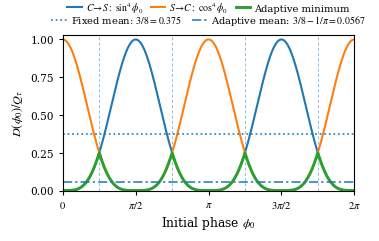
Equations (55) and (69) show that the coefficient multiplying the unknown drift depends on phase. If a predictor for is available from the preceding tracking cycle, the first-order rule is
| (78) |
With perfect prediction, the squared drift coefficient is . Symmetry divides the full phase interval into eight equivalent sectors, or equivalently four copies of . Thus
| (79) | ||||
| (80) | ||||
| (81) | ||||
| (82) |
Therefore
| (83) |
Numerically, the coefficient is 0.05669 rather than 0.375. The relative MSE reduction is
| (84) |
or 84.9%. The corresponding rms reduction is 61.1%.
6.1 Fisher-information interpretation
Assume independent Gaussian quadrature noise with phase-independent variances and . For a measurement , the Fisher information is defined as
| (85) |
Applying Eq. (85) to the cosine and sine quadratures gives
| (86) |
For equal variances, Eq. (78) therefore measures the less informative quadrature first and preserves the more informative quadrature for the end time. With unequal noise variances, the generalized ordering rule is obtained by comparing the full information values and , rather than only and .
7 Increment-aware end-time estimation
7.1 Local phase observations from nonlinear quadratures
The local Gaussian estimator begins by converting a quadrature sample into a phase observation around a predictor . Linearizing the cosine measurement gives
| (87) |
so that
| (88) |
with
| (89) |
Similarly,
| (90) |
These equations make explicit where the local phase observations and Fisher informations enter the estimator.
7.2 Marginalization of the phase increment
Consider the order . The stale and fresh local observations are
| (91) |
with
| (92) |
Rewriting the stale observation in terms of the desired end-time state gives
| (93) |
The two independent terms in parentheses have variances and . Therefore
| (94) |
The information carried by the stale observation about is
| (95) |
The effective information is bounded above by : even an arbitrarily accurate measurement of cannot predict more accurately than the unknown process increment permits.
Combining the independent fresh and stale likelihoods gives
| (96) |
with
| (97) |
For the reverse order,
| (98) |
The information lost when a measurement becomes stale is
| (99) |
Because , delaying a highly informative quadrature is more costly than delaying a weak one. The increment-aware calculation therefore gives the same ordering principle as Section 6.
For equal information, ,
| (100) |
Its limits are
| (101) |
For comparison, a static equal-weight estimator has
| (102) |
which continues to trust the stale measurement even when the uncertainty of the intervening phase change is dominant.
For equal raw quadrature-noise variances, direct already implements the ordinary static Fisher weights to first order. The new factor in Eq. (95) is not a replacement for that geometric weighting; it is the additional loss of information caused by temporal phase evolution.
7.3 Circular nonlinear implementation
The local equations fail near a quadrature extremum and do not represent phase wrapping. The numerical study therefore also uses a circular posterior. For ,
| (103) |
With a uniform circular prior and wrapped-Gaussian transition density ,
| (104) |
The computation used in the simulations consists of four steps. First, the phase interval is sampled on an equally spaced grid. Second, the stale likelihood is propagated to the end time by circular convolution with . Third, the propagated density is multiplied by the fresh likelihood and normalized. Finally, the estimate is the circular posterior mean
| (105) |
On a Fourier grid, propagation is implemented efficiently by multiplying harmonic by . The small-error limit of this circular procedure is Eq. (96).
8 Photon resources and architecture criterion
A spatial–temporal comparison is meaningful only after the optical and detection resources are specified. We first connect the abstract Fisher information used in Section 7 to an ideal shot-noise-limited measurement and then derive receiver-selection boundaries in terms of the phase-increment variance . No particular functional dependence of on the reconfiguration delay is required.
8.1 Ideal balanced photon-counting benchmark
Consider a cosine-quadrature measurement implemented by two complementary photon-counting outputs. Let be the signal photon number incident on this quadrature measurement before detection loss, and let denote the total detection efficiency. The two mean detected counts are
| (106a) | ||||
| (106b) | ||||
The measured counts are modeled as independent Poisson random variables,
| (107) |
For independent Poisson observations, the Fisher information of is
| (108) |
Using
| (109) |
we obtain
| (110) | ||||
| (111) | ||||
| (112) |
The expression at an exactly dark output is understood by continuity. The same calculation for complementary sine outputs,
| (113a) | ||||
| (113b) | ||||
gives
| (114) |
Thus, in the ideal balanced Poisson model, the phase information of each quadrature is independent of phase and equals the detected signal-photon number allocated to that quadrature.
This result is used as a resource benchmark rather than as a detector model for the processor recordings in Section 2, which were obtained from analog power measurements. For an actual receiver, and should be calculated from its measured likelihood or inferred from its calibrated noise statistics.
8.2 Information-gain factor
Let
| (115) |
denote the total Fisher information available to the simultaneous spatial receiver during one complete phase-estimation cycle. The corresponding raw information available to the temporal receiver is
| (116) |
We define the information-gain factor
| (117) |
The case corresponds to equal total information per estimate. Under that convention, temporal readout has no static information advantage and only introduces temporal inconsistency. A value must be justified by the actual architecture, for example through reuse of detector channels, a longer integration assigned to each sequential setting, or concentration of optical power that would otherwise be divided among parallel outputs.
The high-information phase variance of an estimate follows from Eq. (38). Around the unit circle,
| (118) |
and for independent quadrature noises,
| (119) |
If the two quadratures have equal variance , the phase variance is , independent of phase. Equivalently, an efficient receiver with total information has the local benchmark .
8.3 Fixed and adaptive direct readout
Using the total-information convention above, the simultaneous spatial benchmark is
| (120) |
For fixed-order temporal readout, the corresponding leading expression is
| (121) |
Temporal readout is preferable when
| (122) |
The product is dimensionless and expresses the competition between measurement information and the phase uncertainty acquired between settings.
For ideal phase-predicted ordering,
| (123) |
so the corresponding boundary is
| (124) |
Because the adaptive drift coefficient is smaller, it tolerates a larger phase-increment variance for the same static information gain.
8.4 Symmetric local increment-aware boundary
The following boundary is an idealized local benchmark: it assumes that the two local phase observations have equal, phase-independent information. For a symmetric temporal receiver, let each raw quadrature carry information
| (125) |
At the end time, the fresh quadrature retains information , while the stale quadrature contributes . Therefore
| (126) |
For , comparison with Eq. (120) yields
| (127) |
For , the fresh quadrature alone carries the full spatial information, and the stale quadrature provides an additional positive contribution for every finite . For , the fresh temporal quadrature alone exceeds the spatial information in this idealized resource convention. Such cases imply a larger total measurement resource and must therefore be interpreted together with the physical photon, time, and detector constraints.
The fully asymmetric local condition remains
| (128) |
for , with the quadratures exchanged for the reverse order.
Figure 4 presents the three dimensionless boundaries for the same information gain used in the numerical receiver comparison. For this value,
| (129) |
for fixed, increment-aware, and ideal adaptive readout, respectively. Temporal operation is favored below the relevant boundary and spatial operation above it.

8.5 Model scope and detector nonidealities
The ideal photon-counting result in Eqs. (112) and (114) neglects dark counts, background light, afterpulsing, detector dead time, saturation, unequal channel efficiencies, and technical intensity noise. These effects can make the Fisher information phase dependent and can change the resource gain . They should be included through the actual count likelihood or an experimentally calibrated noise model. For analog power detection, the information should likewise be obtained from the measured transfer slopes and covariance of the output powers.
The increment-aware expressions are local and presume that the phase posterior is concentrated around a predictor. When the posterior spans several phase branches or when a quadrature is operated near a locally singular linearization, the circular estimator of Section 7 is required. The quantity should be evaluated for the intended switching interval; the architecture rules depend only on that increment uncertainty and do not require extrapolation to other delays.
9 Monte Carlo validation and design study
For compactness in this section, denotes the phase-increment variance associated with the selected reconfiguration interval. The first numerical study sampled uniformly on , drew , formed the exact mixed-time quadratures, and evaluated Eqs. (34) and (36). The error in each trial was wrapped according to Eq. (37), and the MSE was the average of its square. Each value of used trials.
Figure 5 confirms the fixed-order first-order expression in the small-increment regime. The adaptive result approaches as . At larger , the second-order terms in Eqs. (57) and (71), order-boundary changes, and circular branch effects produce the visible departure from the first-order approximation.

A practical controller selects the order using , with . The second study used so that higher-order drift effects were negligible, and estimated the normalized coefficient from trials per value of . At rad, the coefficient is approximately 0.0631, corresponding to an 83.2% reduction relative to the fixed-order value 0.375. As the prediction becomes uninformative, the order is effectively random and the coefficient returns to the fixed-order limit.

The final study compares complete noisy receiver architectures. It uses
| (130) |
The adaptive receiver uses rad. Direct estimators use trials per point. The circular increment-aware estimator uses a 512-point phase grid and trials per point.
For equal quadrature-noise variances, the information values are and . Equation (122) therefore gives
| (131) |
The exact simulation gives the same fixed-order crossover. The circular increment-aware estimator extends the crossing to approximately 0.0127, while adaptive ordering extends it to approximately 0.0470 for the chosen prediction error and measurement model. The increment-aware value should not be compared directly with the local symmetric prediction from Eq. (127). That boundary assigns the constant information to each local phase observation, whereas the circular simulation starts from noisy sine and cosine samples whose local information varies with phase and vanishes at a quadrature extremum. The exact nonlinear, phase-averaged comparison is therefore more conservative.

10 Conclusion
We developed a detailed theory of spatial and sequential quadrature readout for programmable photonic processors, motivated by the optical transformation and measured phase statistics of an eight-mode processor. The four-port configuration converts the relative phase of inputs 4 and 8 into complementary sine and cosine power pairs, allowing the full phase to be reconstructed from balanced differences.
When the desired estimate is the phase at the completion of the second measurement, fixed-order temporal reconstruction has the first-order errors and . Writing , uniform phase averaging gives the drift MSE . The detailed second-order expansions explain why exact nonlinear simulations depart from the first-order result when the phase increment becomes large.
A phase-predicted ordering rule measures the less informative quadrature first and the more informative one second. Its uniform first-order MSE is , an 84.9% reduction. An increment-aware state-space derivation reaches the same ordering principle and shows that the information of a stale measurement is reduced from to . This correction prevents an estimator from continuing to trust an old phase sample after the uncertainty of the intervening phase change has become dominant.
The resulting crossover conditions separate the possible optical-information advantage of temporal operation from the phase change accumulated during reconfiguration. In an ideal balanced Poisson benchmark, each quadrature contributes Fisher information equal to its detected signal-photon number. The information-gain factor then produces explicit dimensionless boundaries in the product for fixed-order, symmetric local increment-aware, and adaptive readout. Exact Monte Carlo simulations validate the analytical laws, quantify robustness to prediction error, and show the additional limitations introduced by nonlinear quadrature observations. Previously acquired synchronized four-port records provide an empirical route for estimating at a selected delay. A physical implementation with actual sequential reconfiguration would additionally include switching transients, settling behavior, setting-dependent detection noise, and possible power changes between the two measurements.
Acknowledgments
This work was supported by the Federal Ministry of Research, Technology and Space of Germany through the Q-TREX project under Grant 16KISR026 and the QD-CamNetz project under Grant 16KISQ077, and by the Bavarian state government through the Munich Quantum Valley under the Hightech Agenda Bayern Plus.
Disclosures
The authors declare no conflicts of interest.
Data availability
No new experimental data were acquired for this study. The processor recordings analyzed here, together with the simulation code and numerical data supporting the figures, are available from the authors upon reasonable request.
References
- [1] M. Reck, A. Zeilinger, H. J. Bernstein, and P. Bertani, “Experimental realization of any discrete unitary operator,” Physical Review Letters 73, 58–61 (1994), doi: 10.1103/PhysRevLett.73.58.
- [2] W. R. Clements, P. C. Humphreys, B. J. Metcalf, W. S. Kolthammer, and I. A. Walmsley, “Optimal design for universal multiport interferometers,” Optica 3, 1460–1465 (2016), doi: 10.1364/OPTICA.3.001460.
- [3] N. C. Harris, D. Bunandar, M. Pant, G. R. Steinbrecher, J. Mower, M. Prabhu, T. Baehr-Jones, M. Hochberg, and D. Englund, “Large-scale quantum photonic circuits in silicon,” Nanophotonics 5, 456–468 (2016), doi: 10.1515/nanoph-2015-0146.
- [4] J. M. Arrazola, V. Bergholm, K. Brádlér, et al., “Quantum circuits with many photons on a programmable nanophotonic chip,” Nature 591, 54–60 (2021), doi: 10.1038/s41586-021-03202-1.
- [5] Q. Cheng, J. Kwon, M. Glick, M. Bahadori, L. P. Carloni, and K. Bergman, “Silicon photonics codesign for deep learning,” Proceedings of the IEEE 108, 1261–1282 (2020), doi: 10.1109/JPROC.2020.2968184.
- [6] W. Bogaerts, D. Pérez, J. Capmany, et al., “Programmable photonic circuits,” Nature 586, 207–216 (2020), doi: 10.1038/s41586-020-2764-0.
- [7] M. Kuschnerov, K. Piyawanno, M. S. Alfiad, B. Spinnler, A. Napoli, and B. Lankl, “Impact of mechanical vibrations on laser stability and carrier phase estimation in coherent receivers,” IEEE Photonics Technology Letters 22, 1114–1116 (2010), doi: 10.1109/LPT.2010.2050472.
- [8] M. Seimetz, High-Order Modulation for Optical Fiber Transmission. Berlin, Germany: Springer, 2009.
- [9] G. Elmas, I. A. Litvin, P. Kohl, and J. Nötzel, “Modeling and analysis of phase instability in a photonic processor,” Applied Optics 64, 3995–4003 (2025), doi: 10.1364/AO.560370.
- [10] I. A. Litvin, G. Elmas, P. Kohl, and J. Nötzel, “Stable signal processing with a photonic processor,” Journal of Lightwave Technology 43, 9981–9990 (2025), doi: 10.1109/JLT.2025.3606027.
- [11] I. A. Litvin, G. Elmas, K. H. El-Safty, S. Chaudhary, and J. Nötzel, “Robust calibration and energy optimization in reconfigurable photonic processors,” Optics Express 33, 35011–35027 (2025), doi: 10.1364/OE.566817.
- [12] I. A. Litvin, G. Elmas, P. Kohl, and J. Nötzel, “Multi-input signal phase stabilization in photonic processors with on-chip feedback control,” Optics Express 34, 11244–11258 (2026), doi: 10.1364/OE.579969.
- [13] I. A. Litvin, G. Elmas, and J. Nötzel, “Joint detection on reconfigurable photonic processors with multi-input phase stabilization,” IEEE Photonics Journal 18(3), 1–9 (2026), doi: 10.1109/JPHOT.2026.3683204.
- [14] N. C. Harris, J. Carolan, D. Bunandar, M. Prabhu, M. Hochberg, T. Baehr-Jones, M. L. Fanto, A. M. Smith, C. C. Tison, P. M. Alsing, and D. Englund, “Linear programmable nanophotonic processors,” Optica 5, 1623–1631 (2018), doi: 10.1364/OPTICA.5.001623.
- [15] C. Taballione, T. A. W. Wolterink, J. M. Renema, M. S. de Goede, B. J. Metcalf, P. P. Rohde, H. S. M. T. Yung, M. A. de Dood, E. J. Klein, D. J. Broeke, and K.-J. Boller, “88 reconfigurable quantum photonic processor based on silicon nitride waveguides,” Optics Express 27, 26842–26857 (2019), doi: 10.1364/OE.27.026842.
- [16] X. Qiang, X. Zhou, J. Wang, C. M. Wilkes, T. Loke, S. O’Gara, L. Kling, G. D. Marshall, R. Santagati, T. C. Ralph, J. B. Wang, J. L. O’Brien, M. G. Thompson, and J. C. F. Matthews, “Large-scale silicon quantum photonics implementing arbitrary two-qubit processing,” Nature Photonics 12, 534–539 (2018), doi: 10.1038/s41566-018-0236-y.
- [17] J. W. Silverstone, D. Bonneau, J. L. O’Brien, and M. G. Thompson, “Silicon quantum photonics,” IEEE Journal of Selected Topics in Quantum Electronics 22, 390–402 (2016), doi: 10.1109/JSTQE.2016.2573218.
- [18] B. J. Smith, D. Kundys, N. Thomas-Peter, P. G. R. Smith, and I. A. Walmsley, “Phase-controlled integrated photonic quantum circuits,” Optics Express 17, 13516–13525 (2009), doi: 10.1364/OE.17.013516.
- [19] V. Svarc, M. Nováková, M. Dudka, and M. Ježek, “Sub-0.1 degree phase locking of a single-photon interferometer,” Optics Express 31, 12562–12571 (2023), doi: 10.1364/OE.487414.