跳到论文正文
W Papers独立论文阅读器 arXiv:2608.01701 论文正文 计算阅读时间 · 0%
引用这篇论文根据当前论文元数据生成,正式投稿前建议核对。


License: arXiv.org perpetual non-exclusive license
arXiv:2608.01701v1 [hep-ph] 03 Aug 2026

Magnetic field modifications to the pion-quark vertex in the Linear Sigma Model with quarks

Alejandro Ayala1,2,3    Flávia Fialho2    Adrián Lara1    Ana Mizher2    Javier Rendón1 jesus.rendon@correo.nucleares.unam.mx 1Instituto de Ciencias Nucleares, Universidad Nacional Autónoma de México, Apartado Postal 70-543, CdMx 04510, Mexico.
2Instituto de Física, Universidade de São Paulo, Rua do Matão, 1371, CEP 05508-090, São Paulo, SP, Brazil.
3Instituto de Física Teórica, Universidade Estadual Paulista, Rua Dr. Bento Teobaldo Ferraz, 271 - Bloco II, 01140-070 São Paulo, SP, Brazil.
Abstract

We compute the modification to the quark-neutral pion vertex, induced by a constant and uniform magnetic field, using the Linear Sigma Model with quarks as a low energy effective theory of QCD. The vertex is modified even at tree-level since, due to the loss of translational invariance, the calculation should be carried out in configuration space, with the quark described by Ritus wave functions instead of plane waves. We also compute the one-loop vertex modification. These modifications are found for arbitrary Landau levels occupied by the quark. We illustrate the result for the case where the quark occupies the lowest Landau level. To check the result, we also compute the one-loop vertex modification using the Schwinger proper-time method with the quark occupying the lowest Landau level and find the same result as in the case where the Ritus formalism is used.

I Introduction

Vertex corrections are an essential component for the refinement and deeper understanding of field theories. Perturbative calculations become indispensable when aiming to achieve a higher level of theoretical precision and consistency with experimental data. Since Schwinger’s seminal work Schwinger (1948), where the one-loop vertex correction in QED was first computed to extract the vacuum electron anomalous magnetic moment, a systematic framework has been established to calculate perturbatively improved vertices that, together with self-energy calculations, provides a clear interpretation of mass and charge renormalization.

Strong magnetic fields can significantly modify the vacuum properties of particles, both at tree level and through radiative corrections. Radiative effects arise from the magnetic-field-induced modifications of charged-particle propagators appearing in Feynman loops, whereas tree-level effects originate from the proper description of asymptotic charged states in terms of the Ritus eigenfunctions Ritus (1978), instead of the plane waves that characterize the field-free theory. Strong magnetic fields are predicted to be generated in a variety of physical settings, including heavy-ion collisions Kharzeev et al. (2008); Skokov et al. (2009); Voronyuk et al. (2011), astrophysical compact objects such as magnetars Duncan and Thompson (1992); Kouveliotou and others (1998), and the early universe Grasso and Rubinstein (2001). Strong magnetic fields also provide a powerful probe for studying the properties of the QCD vacuum. For example, at zero temperature, it is well known that magnetic fields catalyze the breaking of chiral symmetry Gusynin et al. (1999), even for weak magnetic fields Ayala et al. (2006), a phenomenon referred to as magnetic catalysis. However, at nonzero temperatures, magnetic fields suppress condensate formation and lower the critical temperature for chiral symmetry restoration, leading to the phenomenon known as inverse magnetic catalysis Bali et al. (2012a, b); Bruckmann et al. (2013); Farias et al. (2014); Ferreira et al. (2014); Ayala et al. (2015c, b, 2014); Farias et al. (2017); Ayala et al. (2016); Ferrer et al. (2015); Ayala et al. (2015a, 2018); Mueller et al. (2014); Mueller and Pawlowski (2015); Bandyopadhyay and Farias (2021).

Modifications of the interaction vertices in weak processes induced by strong magnetic fields have been computed at tree-level for the leptonic decays of charged pions by analyzing their decay widths in Refs. Nikishov and Ritus (1964a, b); Bali et al. (2018); Coppola et al. (2019, 2020b, 2020a). The quark anomalous magnetic moment (AMM) in an extreme magnetic background from perturbative QCD has recently been computed in Ref. Fraga et al. (2024). In addition, the one-loop correction to the electron AMM has been improved by taking into account magnetic field corrections in the weak field limit Lin and Huang (2022). An earlier result for the electron AMM in the presence of magnetic fields was found in Ref. Baier and Katkov (2001). A more general calculation of the magnetic field induced modifications of the QED vertex, including the analysis of the purely transverse contribution to the fermion AMM for arbitrary Landau levels, has been recently performed in Ref. Ayala et al. (2026). Consequences of a magnetic field-dependent quark AMM have been explored in Refs. Tavares et al. (2024); Farias et al. (2022); Fayazbakhsh and Sadooghi (2014). More recently, the strong magnetic field modifications of the neutral pion decay width have also been studied in Ref. Coppola et al. (2025) using the Nambu–Jona-Lasinio model and in Refs. Brauner and Kadam (2017); Adhikari and Tiburzi (2024) using chiral perturbation theory and in Refs. Ayala et al. (2020, 2021), approximations to the magnetic corrections of the boson self-coupling and boson-fermion coupling in the linear sigma model with quarks (LSMq).

Motivated by these developments, here we compute both the general expressions for the tree-level and one-loop magnetic-field-induced corrections to the quark-neutral pion-quark vertex, within the LSMq. We present explicit results for the case of the u​π0​uu\pi^{0}u case. These corrections are relevant for describing scattering processes in a magnetized medium, for systems undergoing spontaneous chiral symmetry restoration, and for decay processes influenced by the presence of an external magnetic field. The work is structured as follows: In Sec. II, we summarize the ingredients of the LSMq. In Sec. III, we discuss the form of the propagators for the charged particles of the model, both in the Ritus and Schwinger’s proper time formalisms. In Sec. IV, we use the Ritus formalism to perform the calculations that correspond to the quark-neutral pion vertex correction for an arbitrary strength of the magnetic field, at tree-level in Sec. IV.1, and at one-loop level in Sec. IV.2, for arbitrary Landau levels occupied by the quark. We illustrate the calculation, showing the result explicitly in the lowest Landau level (LLL). In Sec. V we perform the vertex correction at one-loop level, starting explicitly from the quark in the LLL using the Ritus formalism. In Sec. VI, we independently evaluate the same one-loop correction in the LLL using Schwinger’s proper-time formalism and demonstrate the equivalence between both approaches. In Sec. VII we present the numerical results for the case when the quark occupies the lowest Landau level (LLL). We finally summarize and conclude in Sec. VIII and leave for the appendices the explicit computation of the integrals involved, as well as the derivation of some of the elements required in the calculation.

II Linear Sigma Model with quarks

The S​U​(2)×S​U​(2)SU(2)\times SU(2) LSMq is an effective theory of QCD that includes quarks together with the lightest scalar and pseudoscalar mesons as explicit degrees of freedom. It incorporates chiral symmetry breaking and is particularly well-suited for studying hadronic physics in the light-meson sector. The Lagrangian is given by

ℒ\displaystyle\mathcal{L} =\displaystyle= 12​(∂μσ)2+12​(∂μπ→)2+a22​(σ2+π→2)−λ4​(σ2+π→2)2\displaystyle\frac{1}{2}(\partial_{\mu}\sigma)^{2}+\frac{1}{2}(\partial_{\mu}\vec{\pi})^{2}+\frac{a^{2}}{2}(\sigma^{2}+\vec{\pi}^{2})-\frac{\lambda}{4}(\sigma^{2}+\vec{\pi}^{2})^{2} (1)
+\displaystyle+ i​ψ¯​γμ​∂μψ−i​g​γ5​ψ¯​τ→⋅π→​ψ−g​ψ¯​ψ​σ,\displaystyle i\bar{\psi}\gamma^{\mu}\partial_{\mu}\psi-ig\gamma^{5}\bar{\psi}\vec{\tau}\cdot\vec{\pi}\psi-g\bar{\psi}\psi\sigma\,,

where π→=(π1,π2,π3)\vec{\pi}=(\pi_{1},\pi_{2},\pi_{3}) represents an isospin triplet, ψ=(u,d)\psi=(u,d) represents an isospin doublet, and the σ\sigma scalar is an isospin singlet. The parameters λ\lambda and gg correspond to the boson self-coupling and the boson-fermion coupling, respectively.
After spontaneous symmetry breaking, the σ\sigma field becomes

σ→σ+v.\sigma\rightarrow\sigma+v\,. (2)

As a consequence of this shift, the Lagrangian ℒ\mathcal{L} reads

ℒ\displaystyle\mathcal{L} =\displaystyle= 12​∂μσ​∂μσ+12​∂μπ0​∂μπ0+∂μπ−​∂μπ+\displaystyle\frac{1}{2}\partial_{\mu}\sigma\partial^{\mu}\sigma+\frac{1}{2}\partial_{\mu}\pi_{0}\partial^{\mu}\pi_{0}+\partial_{\mu}\pi_{-}\partial^{\mu}\pi_{+} (3)
−\displaystyle- 12​mσ2​σ2−12​m02​π02−m02​π−​π++i​ψ¯​∂̸ψ\displaystyle\frac{1}{2}m_{\sigma}^{2}\sigma^{2}-\frac{1}{2}m_{0}^{2}\pi_{0}^{2}-m_{0}^{2}\pi_{-}\pi_{+}+i\bar{\psi}\not{\partial}\psi
−\displaystyle- mf​ψ¯​ψ+a22​v2−λ4​v4+h​v+ℒi​n​t,\displaystyle m_{f}\bar{\psi}\psi+\frac{a^{2}}{2}v^{2}-\frac{\lambda}{4}v^{4}\ +\ hv+\mathcal{L}_{int},

where h​vhv represents an explicit symmetry breaking term to give the pions a finite mass. The charged-pion fields are defined as

π±=12​(π1∓i​π2),\pi_{\pm}=\frac{1}{\sqrt{2}}(\pi_{1}\mp i\pi_{2}), (4)

and the interaction Lagrangian takes the form

ℒi​n​t=−λ4​σ4−λ​v​σ3−λ​v3​σ−λ​σ2​π−​π+−2​λ​v​σ​π−​π+−λ2​σ2​π02−λ​v​σ​π02−λ​π−2​π+2−λ​π−​π+​π02−λ4​π04+a2​v​σ−g​ψ¯​ψ​σ−i​g​γ5​ψ¯​(τ+​π++τ−​π−+τ3​π0)​ψ.\begin{split}\mathcal{L}_{int}&=-\frac{\lambda}{4}\sigma^{4}-\lambda v\sigma^{3}-\lambda v^{3}\sigma-\lambda\sigma^{2}\pi_{-}\pi_{+}-2\lambda v\sigma\pi_{-}\pi_{+}\\ &-\frac{\lambda}{2}\sigma^{2}\pi_{0}^{2}-\lambda v\sigma\pi_{0}^{2}-\lambda\pi_{-}^{2}\pi_{+}^{2}-\lambda\pi_{-}\pi_{+}\pi_{0}^{2}-\frac{\lambda}{4}\pi_{0}^{4}\\ &+a^{2}v\sigma-g\bar{\psi}\psi\sigma-ig\gamma^{5}\bar{\psi}\left(\tau_{+}\pi_{+}+\tau_{-}\pi_{-}+\tau_{3}\pi_{0}\right)\psi.\end{split} (5)

The masses appearing in Eq. (3) are explicitly given by

mσ2\displaystyle m_{\sigma}^{2} =3​λ​v2−a2,\displaystyle=3\lambda v^{2}-a^{2},
m02\displaystyle m_{0}^{2} =λ​v2−a2,\displaystyle=\lambda v^{2}-a^{2},
mf\displaystyle m_{f} =g​v.\displaystyle=gv. (6)

We introduce the effect of an external magnetic field 𝐁\mathbf{B} through a covariant derivative in the Lagrangian density in Eq. (3), that is

∂μ→Dμ=∂μ+i​e​Aμ,\partial_{\mu}\to D_{\mu}=\partial_{\mu}+ieA_{\mu}, (7)

where AμA^{\mu} is the vector potential that couples a charged particle with the external magnetic field. In this work, we take this field to be uniform in space and constant in time, choosing the zz-axis as its direction.

III Magnetic field-dependent propagators

The charged particle propagators are modified in the presence of a background magnetic field. In this section, we summarize the explicit expressions for the scalar and fermion propagators immersed in the magnetic field. Their representations are provided both in the Ritus basis and in the Schwinger proper-time formalism.

We start by discussing the Schwinger proper-time formalism, and then discuss the Ritus representation. Although not directly used in this work, for completeness, we first present the scalar charged propagator, which can be written as

Db​(x,x′)=ei​ΦP​(x,x′)​Db​(x−x′),D_{b}(x,x^{\prime})=e^{i\Phi_{P}(x,x^{\prime})}D_{b}(x-x^{\prime})\,, (8)

where the Schwinger phase ΦP​(x,x′)\Phi_{P}(x,x^{\prime}) is defined as

ΦP​(x,x′)=QP​∫xx′𝑑ξμ​[Aμ​(ξ)+12​Fμ​ν​(ξ−x′)ν],\displaystyle\Phi_{P}(x,x^{\prime})=Q_{P}\int_{x}^{x^{\prime}}d\xi_{\mu}\left[A^{\mu}(\xi)+\frac{1}{2}F^{\mu\nu}(\xi-x^{\prime})_{\nu}\right], (9)

and QPQ_{P} denotes the electric charge of a particle PP. The translationally and gauge invariant part of the propagator Db​(x−x′)D_{b}(x-x^{\prime}) can be written in terms of its Fourier transform as

Db​(x−x′)=∫d4​p(2​π)4​Db​(p)​e−i​p⋅(x−x′)D_{b}(x-x^{\prime})=\int\frac{d^{4}p}{(2\pi)^{4}}D_{b}(p)e^{-ip\cdot(x-x^{\prime})} (10)

where

i​Db​(p)\displaystyle iD_{b}(p) =\displaystyle= ∫0∞d​scos⁡(|qb​B|​s)​ei​s​(p∥2−p⟂2​tan⁡(|qb​B|​s)|qb​B|​s−mb2+i​ϵ).\displaystyle\int_{0}^{\infty}\frac{ds}{\cos(|q_{b}B|s)}e^{is\left(p_{\parallel}^{2}-p_{\perp}^{2}\frac{\tan(|q_{b}B|s)}{|q_{b}B|s}-m_{b}^{2}+i\epsilon\right)}\,.

The scalar propagator can also be written in terms of Ritus functions as

Db​(x,y)=\sumintq¯​ℱQ⁡(x,q¯)​Db​(k,q∥)​ℱQ¯​(y,q¯)D_{b}(x,y)=\sumint_{\bar{q}}\operatorname{\mathcal{F}}^{Q}(x,\bar{q})D_{b}(k,q_{\parallel})\bar{\operatorname{\mathcal{F}}^{Q}}(y,\bar{q}) (12)

where in the Landau gauge 2 (LG2) we have

\sumintq¯=12​π​∫d​q02​π​d​q22​π​d​q32​π,\sumint_{\bar{q}}=\frac{1}{2\pi}\int\frac{dq_{0}}{2\pi}\frac{dq_{2}}{2\pi}\frac{dq_{3}}{2\pi}\,, (13)

and

Db​(k,q∥)=1q∥2−mb2−(2​k+1)​BQ+i​ϵD_{b}(k,q_{\parallel})=\frac{1}{q_{\parallel}^{2}-m_{b}^{2}-(2k+1)B_{Q}+i\epsilon} (14)

with BQ=|q​B|B_{Q}=|qB|. The Ritus functions ℱQ⁡(x,q¯)\operatorname{\mathcal{F}}^{Q}(x,\bar{q}) that appear in Eq. (12) can be explicitly written in the LG2 as

ℱQ⁡(x,q¯)\displaystyle\operatorname{\mathcal{F}}^{Q}(x,\bar{q}) =\displaystyle= Nk​e−i​(q0​x0−q2​x2−x3​x3)\displaystyle N_{k}e^{-i(q_{0}x_{0}-q_{2}x_{2}-x_{3}x_{3})} (15)
×\displaystyle\times Dk​(2​BQ​(x1−s​q2BQ)),\displaystyle D_{k}\left(\sqrt{2B_{Q}}\left(x_{1}-\frac{sq_{2}}{B_{Q}}\right)\right)\,,

where

Nk\displaystyle N_{k} =\displaystyle= (4​π​BQ)1/4/k!,\displaystyle(4\pi B_{Q})^{1/4}/\sqrt{k!},
Dk​(x)\displaystyle D_{k}(x) =\displaystyle= 2−k/2​e−x2/4​Hk​(x/2),\displaystyle 2^{-k/2}e^{-x^{2}/4}H_{k}(x/\sqrt{2}), (16)

with HkH_{k} the Hermite polynomial of degree kk. We also use the definition q¯=(q0,k,q2,q3)\bar{q}=(q_{0},k,q_{2},q_{3}).

We now present the corresponding results for the fermion propagator. Once again, we begin with Schwinger’s proper-time formalism. The fermion propagator can be written as

Sf​(x,x′)=ei​ΦP​(x,x′)​Sf​(x−x′),S_{f}(x,x^{\prime})=e^{i\Phi_{P}(x,x^{\prime})}S_{f}(x-x^{\prime}), (17)

where the translationally and gauge invariant part Sf​(x−x′)S_{f}(x-x^{\prime}) is given by

Sf​(x−x′)=∫d4​p(2​π)4​Sf​(p)​e−i​p⋅(x−x′),S_{f}(x-x^{\prime})=\int\frac{d^{4}p}{(2\pi)^{4}}S_{f}(p)e^{-ip\cdot(x-x^{\prime})}, (18)

with

i​Sf​(p)\displaystyle iS_{f}(p) =\displaystyle= ∫0∞d​scos⁡(|qf​B|​s)​ei​s​(p∥2−p⟂2​tan⁡(|qf​B|​s)|qf​B|​s−mf2+i​ϵ)\displaystyle\int_{0}^{\infty}\frac{ds}{\cos(|q_{f}B|s)}e^{is\left(p_{\parallel}^{2}-p_{\perp}^{2}\frac{\tan(|q_{f}B|s)}{|q_{f}B|s}-m_{f}^{2}+i\epsilon\right)} (19)
×\displaystyle\times [(cos⁡(|qf​B|​s)+γ1γ2sin⁡(|qf​B|​s)sign(qfB))\displaystyle\left[\Big(\cos(|q_{f}B|s)+\gamma_{1}\gamma_{2}\sin(|q_{f}B|s)\text{sign}(q_{f}B)\Big)\right.
×\displaystyle\times (mf+p̸∥)−p̸⟂cos⁡(|qf​B|​s)].\displaystyle\left.\left(m_{f}+\not{p}_{\parallel}\right)-\frac{\not{p}_{\perp}}{\cos(|q_{f}B|s)}\right].

In terms of Ritus functions we can also write the fermion propagator as

Sf​(x,y)=\sumintq¯​𝔼Q⁡(x,q¯)​Sf​(k,q∥)​𝔼¯Q​(y,q¯)S_{f}(x,y)=\sumint_{\bar{q}}\operatorname{\mathbb{E}}^{Q}(x,\bar{q})S_{f}(k,q_{\parallel})\bar{\operatorname{\mathbb{E}}}^{Q}(y,\bar{q}) (20)

where

Sf​(k,q∥)=Π̸s+mfq∥2−mf2−2​k​BQ,S_{f}(k,q_{\parallel})=\frac{\not{\Pi}_{s}+m_{f}}{q_{\parallel}^{2}-m_{f}^{2}-2kB_{Q}}\,, (21)

with Πsμ=(q0,0,−s​2​k​BQ,q3)\Pi_{s}^{\mu}=(q_{0},0,-s\sqrt{2kB_{Q}},q_{3}).
The Ritus functions 𝔼Q⁡(x,q¯)\operatorname{\mathbb{E}}^{Q}(x,\bar{q}) appearing in Eq. (20) are given by

𝔼Q⁡(x,q¯)=∑λ=±Δλ​ℱQ⁡(x,q¯λ)\operatorname{\mathbb{E}}^{Q}(x,\bar{q})=\sum_{\lambda=\pm}\Delta^{\lambda}\operatorname{\mathcal{F}}_{Q}(x,\bar{q}_{\lambda}) (22)

and

𝔼¯Q(y,q¯)=γ0𝔼Q(y,q¯)†γ0{\bar{\operatorname{\mathbb{E}}}^{Q}}(y,\bar{q})=\gamma^{0}{\operatorname{\mathbb{E}}}^{Q}(y,\bar{q})^{\dagger}\gamma^{0} (23)

with Δλ=(1+i​λ​γ1​γ2)/2\Delta^{\lambda}=(1+i\lambda\gamma^{1}\gamma^{2})/2. In the LG2 q¯λ=(q0,ks​λ,q2,q3)\overline{q}_{\lambda}=(q_{0},k_{s\lambda},q_{2},q_{3}) with ks​λ=k−(1−s​λ)/2k_{s\lambda}=k-(1-s\lambda)/2, with the function ℱQ⁡(x,q¯)\operatorname{\mathcal{F}}_{Q}(x,\bar{q}), given by Eq. (15).

IV Vertex corrections

In this section, we analyze the vertex modifications induced by the magnetic field for the neutral pion and a quark, that for definitiveness, we take as uu. We perform the calculation both at tree- and at one-loop level, following closely the notation of Refs. Gomez Dumm et al. (2023); Coppola et al. (2019).

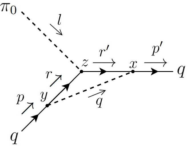
Refer to caption
Figure 1: Feynman diagram corresponding to the tree-level magnetic modification of the π0​q​q\pi_{0}qq vertex, represented by the blob joining the π0\pi_{0} and the qq lines.

IV.1 TREE LEVEL VERTEX CORRECTION

The amplitude for the process u+π0→uu+\pi_{0}\rightarrow u at tree-level which corresponds to the Feynman diagram of Fig. 1 is given by

𝒱=⟨u|i​∫d4​x​ℒi​n​t​(x)|u​π0⟩,\mathcal{V}=\langle{u}|\ i\int d^{4}x\mathcal{L}_{int}(x)|u\pi_{0}\rangle\,, (24)

for which the interaction Lagrangian ℒi​n​t​(x)\mathcal{L}_{int}(x) is,

ℒi​n​t​(x)=−i​g​u¯​γ5​u​π0.\mathcal{L}_{int}(x)=-ig\bar{u}\gamma^{5}u\pi_{0}\,. (25)

The expansion for the quark field in terms of creation and annihilation operators has the form

ψ​(x)\displaystyle\!\!\!\!\!\!\!\psi(x) =\displaystyle\!\!\!=\!\!\!\!\! \sumint{q¯​EQ}​12​EQ\displaystyle\sumint_{\{\bar{q}E_{Q}\}}\frac{1}{2E_{Q}} (26)
×\displaystyle\!\!\!\times\!\!\! ∑a=1,2{b​(q˘,a)​U​(x,q¯,a)+d†​(q˘,a)​V​(x,q¯,a)},\displaystyle\sum_{a=1,2}\left\{b(\breve{q},a)U(x,\bar{q},a)+d^{\dagger}(\breve{q},a)V(x,\bar{q},a)\right\},

where the quark energy is given by

EQ=m2+2​k​BQ+(q3)2,\displaystyle E_{Q}=\sqrt{m^{2}+2kB_{Q}+(q_{3})^{2}}, (27)

with k≥0k\geq 0, and q˘=(k,q2,q3)\breve{q}=(k,q_{2},q_{3}), also we have used the shorthand notation

\sumint{q¯​EQ}=\sumintq¯​2​π​δ​(q0−EQ).\sumint_{\{\bar{q}E_{Q}\}}=\sumint_{\bar{q}}2\pi\delta(q_{0}-E_{Q})\,. (28)

This expression depends on the choice of gauge and working in the LG2, it explicitly looks like

\sumintq¯≡12​π​∑k=0∞∫d​q02​π​d​q22​π​d​q32​π.\sumint_{\bar{q}}\equiv\frac{1}{2\pi}\sum_{k=0}^{\infty}\int\frac{dq_{0}}{2\pi}\frac{dq_{2}}{2\pi}\frac{dq_{3}}{2\pi}\,. (29)

The corresponding expansion for the neutral pion field in terms of creation and annihilation operators is

π0​(x)=∫d4​p(2​π)4​2​π​δ​(p0−Eπ)2​Eπ​(ap​e−i​p⋅x+ap†​ei​p⋅x),\pi_{0}(x)=\int\frac{d^{4}p}{(2\pi)^{4}}\frac{2\pi\delta(p_{0}-E_{\pi})}{2E_{\pi}}(a_{p}e^{-ip\cdot x}+a_{p}^{\dagger}e^{ip\cdot x})\,, (30)

where the pion energy is given by Eπ=|p→|2+mπ2E_{\pi}=\sqrt{|\vec{p}|^{2}+m^{2}_{\pi}}.

Canonical quantization imposes the following anti-commutation relations for the quark fields

{b​(q˘,a),b​(q˘′,a′)}\displaystyle\{b(\breve{q},a),b(\breve{q}^{\prime},a^{\prime})\} =\displaystyle= {d​(q˘,a),d​(q˘′,a′)}=0,\displaystyle\{d(\breve{q},a),d(\breve{q}^{\prime},a^{\prime})\}=0,
{b​(q˘,a),d​(q˘′,a′)}\displaystyle\{b(\breve{q},a),d(\breve{q}^{\prime},a^{\prime})\} =\displaystyle= {b​(q˘,a),d​(q˘′,a′)†}=0,\displaystyle\{b(\breve{q},a),d(\breve{q}^{\prime},a^{\prime})^{\dagger}\}=0,
{b​(q˘,a),b​(q˘′,a′)†}\displaystyle\{b(\breve{q},a),b(\breve{q}^{\prime},a^{\prime})^{\dagger}\} =\displaystyle= 2​EQ​(2​π)3​δχ​χ′​δa​a′​δk​k′​δ​(q3−q′3)\displaystyle 2E_{Q}(2\pi)^{3}\delta_{\chi\chi^{\prime}}\delta_{aa^{\prime}}\delta_{kk^{\prime}}\delta(q_{3}-{q^{\prime}}_{3})
{d​(q˘,a),d​(q˘′,a′)}†\displaystyle\{d(\breve{q},a),d(\breve{q}^{\prime},a^{\prime})\}^{\dagger} =\displaystyle= 2​EQ​(2​π)3​δχ​χ′​δa​a′​δk​k′​δ​(q3−q′3),\displaystyle 2E_{Q}(2\pi)^{3}\delta_{\chi\chi^{\prime}}\delta_{aa^{\prime}}\delta_{kk^{\prime}}\delta(q_{3}-{q^{\prime}}_{3}),

and the commutation relations for the pion field

=[ap†,ap′†]=0,=2Eπ(2π)3δ(3)(p→−p→′). \begin{gathered}=[a_{p}^{\dagger},a_{p^{\prime}}^{\dagger}]=0\,,\\ =2E_{\pi}(2\pi)^{3}\delta^{(3)}(\vec{p}-\vec{p}^{\prime})\,.{}\end{gathered} (32)

Notice that the quark field expansion in Eq. (26) is expressed in terms of Ritus eigenfunctions, as these correspond to charged states, whereas the pion field expansion in Eq. (30) is written in terms of plane waves, reflecting its neutral nature. The commutation relations in Eq. (32) are the standard ones. In contrast, the anti-commutation relations in Eq. (LABEL:quark_commutation) explicitly depend on the choice of gauge, reflecting once again the charged nature of the corresponding particles.

Inserting the interaction Lagrangian together with the expansion of the fields into Eq. (24), and using the commutation and anti-commutation rules, we obtain the following expression for the tree-level vertex

𝒱 (tree)=−g​∫d4​x​U¯​(x,p¯′,a′)​γ5​U​(x,p¯,a)​e−i​l⋅x,\mathcal{V}^{\mbox{\small{ (tree)}}}=-g\int d^{4}x\,\bar{U}(x,\bar{p}^{\prime},a^{\prime})\gamma^{5}{U}(x,\bar{p},a)e^{-il\cdot x}\,, (33)

where the explicit expression for U​(x,p¯,a)U(x,\bar{p},a) is given by

U​(x,p¯,a)=𝔼Q⁡(x,p¯)​uQ​(k,x3,a),\begin{gathered}U(x,\bar{p},a)=\operatorname{\mathbb{E}}^{Q}(x,\bar{p})u_{Q}(k,x_{3},a),\end{gathered} (34)

and the spinor uQ​(k,x3,a)u_{Q}(k,x_{3},a) is written as

uQ​(k,x3,a)=[Π̸s​(EQ,k,x3)+mf​ℐ]2​(EQ+m)​(ϕ(a)ϕ(a)).u_{Q}(k,x_{3},a)\!=\!\frac{\left[\not{\Pi}_{s}(E_{Q},k,x_{3})\!+\!m_{f}\mathcal{I}\right]}{\sqrt{2(E_{Q}+m)}}\begin{pmatrix}\phi^{(a)}\\ \phi^{(a)}\end{pmatrix}. (35)

For completeness, we also write the expression for the negative energy solution

V​(x,p¯′,a)=𝔼~−Q​(x,p¯′)​v−Q​(k,x3,a).V(x,\bar{p}^{\prime},a)=\tilde{\operatorname{\mathbb{E}}}^{-Q}(x,\bar{p}^{\prime})v_{-Q}(k,x_{3},a)\,. (36)

where

v−Q​(k,x3,a)=[−Π̸−s​(EQ,k,x3)+mf​ℐ]2​(EQ+m)​(ϕ~(a)−ϕ~(a)),v\!_{-Q}(k,\!x_{3},\!a)\!=\!\frac{\left[\!-\not{\Pi}_{\!-s}(E_{Q},k,x_{3})\!+\!m_{f}\mathcal{I}\right]}{\sqrt{2(E_{Q}\!+\!m)}}\begin{pmatrix}\!\!\tilde{\phi}^{(a)}\\ -\tilde{\phi}^{(a)}\!\!\end{pmatrix}, (37)
Refer to caption
Figure 2: Feynman diagram corresponding to the one-loop magnetic modification of the π0​q​q¯\pi_{0}q\bar{q} vertex.

with ϕ(1)⁣†=−ϕ~(2)⁣†=(1,0)\phi^{(1)\dagger}=-\tilde{\phi}^{(2)\dagger}=(1,0), ϕ(2)⁣†=ϕ~(1)⁣†=(0,1)\phi^{(2)\dagger}=\tilde{\phi}^{(1)\dagger}=(0,1) and Πsμ​(q0,k,q3)=(q0,0,−s​2​k​BQ,q3)\Pi_{s}^{\mu}(q_{0},k,q_{3})=(q_{0},0,-s\sqrt{2kB_{Q}},q_{3}). The Weyl representation for the Dirac matrices is used in this work,

γ0=(0ℐℐ0)γ→=(0σ→−σ→0).\gamma_{0}=\begin{pmatrix}0&\mathcal{I}\\ \mathcal{I}&0\\ \end{pmatrix}\qquad\vec{\gamma}=\begin{pmatrix}0&\vec{\sigma}\\ -\vec{\sigma}&0\\ \end{pmatrix}. (38)

Notice that Eq. (34) contains the Ritus function 𝔼Q⁡(x,p¯)\operatorname{\mathbb{E}}^{Q}(x,\bar{p}), previously defined in Eq. (22). For completeness, we also write the function 𝔼~−Q​(x,p¯′)\tilde{\operatorname{\mathbb{E}}}^{-Q}(x,\bar{p}^{\prime}), given by Ritus (1978)

𝔼~−Q​(x,p¯′)=∑λ=±Δλ​ℱ−Q∗⁡(x,p¯−λ′),\tilde{\operatorname{\mathbb{E}}}^{-Q}(x,\bar{p}^{\prime})=\sum_{\lambda=\pm}\Delta^{\lambda}\operatorname{\mathcal{F}}^{*}_{-Q}(x,\bar{p}^{\prime}_{-\lambda}), (39)

with the function ℱQ⁡(x,q¯)\operatorname{\mathcal{F}}_{Q}(x,\bar{q}) defined in Eq. (15). Inserting the explicit forms for U¯​(x,p¯,a)\bar{U}(x,\bar{p},a) and U​(x,p¯′,a′){U}(x,\bar{p}^{\prime},a^{\prime}) in Eq. (33) we can write the vertex 𝒱(tree)\mathcal{V}^{\mbox{\small{(tree)}}} as

𝒱 (tree)=−g​u¯Q​ξ​(p¯,p¯′,l)​uQ,\mathcal{V}^{\mbox{\small{ (tree)}}}=-g\bar{u}_{Q}\xi(\bar{p},\bar{p}^{\prime},l)u_{Q}\,, (40)

where

ξ​(p¯,p¯′,l)\displaystyle\xi(\bar{p},\!\bar{p}^{\prime}\!,\!l)\! =\displaystyle= γ5​∑λ=±Δλ​(2​π)3​δ2​(p∥′−p∥−l∥)​δ​(p2′−p2−l2)\displaystyle\!\gamma^{5}\!\sum_{\lambda=\pm}\!\Delta^{\lambda}(2\pi)^{3}\delta^{2}(p^{\prime}_{\parallel}\!-p_{\parallel}\!-\!l_{\parallel})\delta(p^{\prime}_{2}\!-\!p_{2}\!-\!l_{2}) (41)
×\displaystyle\times 𝒥​(ks​λ,ks​λ′),\displaystyle\mathcal{J}(k_{s\lambda},k^{\prime}_{s\lambda}),

with

𝒥​(ks​λ,ks​λ′)=ei​s​l1​(p′⁣2+p2)2​BQ​𝒢ks​λ,ks​λ′​(l⟂),\mathcal{J}(k_{s\lambda},k^{\prime}_{s\lambda})=e^{is\frac{l^{1}(p^{\prime 2}+p^{2})}{2B_{Q}}}\mathcal{G}_{k_{s\lambda},k^{\prime}_{s\lambda}}(l_{\perp})\,, (42)

and

𝒢ks​λ,ks​λ′​(l⟂)\displaystyle\mathcal{G}_{k_{s\lambda},k^{\prime}_{s\lambda}}(l_{\perp}) =\displaystyle\!\!=\!\! 2​π​iks​λ−ks​λ′​ks​λ′!ks​λ!​(l⟂22​BQ)ks​λ−ks​λ′2\displaystyle 2\pi i^{k_{s\lambda}-k^{\prime}_{s\lambda}}\sqrt{\frac{k^{\prime}_{s\lambda}!}{k_{s\lambda}!}}\left(\frac{l_{\perp}^{2}}{2B_{Q}}\right)^{\frac{k_{s\lambda}-k^{\prime}_{s\lambda}}{2}} (43)
×\displaystyle\!\!\times\!\! e−l⟂24​|BQ|​ei​s​ϕ⟂​(ks​λ−ks​λ′)\displaystyle e^{-\frac{l^{2}_{\perp}}{4|B_{Q}|}}e^{is\phi_{\perp}(k_{s\lambda}-k^{\prime}_{s\lambda})}
×\displaystyle\!\!\times\!\! Lks​λ′ks​λ−ks​λ′​(l⟂22​BQ).\displaystyle L_{k^{\prime}_{s\lambda}}^{k_{s\lambda}-k^{\prime}_{s\lambda}}\left(\frac{l_{\perp}^{2}}{2B_{Q}}\right).

Equation (41), together with the functions defined in Eqs. (42) and (43), represents the tree-level modification to the point-like π0​q​q\pi_{0}qq. Since, in the presence of the magnetic field, overall momentum is not conserved, the modification is written as a Gaussian form factor in the transverse direction, modulated by a Laguerre polynomial that depends on the quark Landau levels. The modified vertex also depends on the polarization state of the quark pair. We thus see that the vertex is modified even at tree-level. However, in order to get a more precise perturbative picture of the vertex modifications induced by the magnetic field, we now proceed to compute the one-loop correction.

IV.2 One-loop vertex

The Feynman diagram representing the one-loop π0​q​q\pi_{0}qq vertex is shown in Fig. 2. Its explicit expression is given by

𝒱 (1)=i3​∫d4​x​d4​y​d4​z​U¯​(p′,x)​(−i​g​γ5)​Sf​(x,z)​(−i​g​γ5)​Sf​(z,y)​(−i​g​γ5)​D​(y,x)​U​(y,p)​e−i​l⋅z.\mathcal{V}^{\mbox{\small{ (1)}}}=i^{3}\int d^{4}xd^{4}yd^{4}z\bar{U}(p^{\prime},x)(-ig\gamma^{5})S_{f}(x,z)(-ig\gamma^{5})S_{f}(z,y)(-ig\gamma^{5})D(y,x)U(y,p)e^{-il\cdot z}. (44)

Using Eqs. (20), (21) and (34) into Eq. (44) we can write 𝒱(1)\mathcal{V}^{\mbox{\small{(1)}}} as

𝒱 (1)=i​g3​∫d4​x​d4​y​d4​z​\sumintr¯​\sumintr′¯​∫d4​q(2​π)4​e−i​q⋅(y−x)​e−i​l⋅z(r∥2−m2−2​k1​BQ)​(r∥′⁣2−m2−2​k2​BQ)​(q2−mπ2)\displaystyle\mathcal{V}^{\mbox{\small{ (1)}}}=ig^{3}\int d^{4}xd^{4}yd^{4}z\sumint_{\bar{r}}\sumint_{\bar{r^{\prime}}}\int\frac{d^{4}q}{(2\pi)^{4}}\frac{e^{-iq\cdot(y-x)}e^{-il\cdot z}}{(r_{\parallel}^{2}-m^{2}-2k_{1}B_{Q})(r_{\parallel}^{\prime 2}-m^{2}-2k_{2}B_{Q})(q^{2}-m_{\pi}^{2})} (45)
u¯​(k′,p′,a′)​𝔼¯Q​(x,p′¯)​𝔼Q⁡(x,r′¯)​(Π̸s​(r′¯)−m)​γ5​𝔼¯Q​(z,r′¯)​𝔼Q⁡(z,r¯)​(Π̸s​(r¯)−m)​𝔼¯Q​(y,r¯)​𝔼¯Q​(y,p¯)​u​(k,p,a)\displaystyle\bar{u}(k^{\prime},p^{\prime},a^{\prime})\bar{\operatorname{\mathbb{E}}}^{Q}(x,\bar{p^{\prime}})\operatorname{\mathbb{E}}^{Q}(x,\bar{r^{\prime}})(\not{\Pi}_{s}(\bar{r^{\prime}})-m)\gamma^{5}\bar{\operatorname{\mathbb{E}}}^{Q}(z,\bar{r^{\prime}})\operatorname{\mathbb{E}}^{Q}(z,\bar{r})(\not{\Pi}_{s}(\bar{r})-m)\bar{\operatorname{\mathbb{E}}}^{Q}(y,\bar{r})\bar{\operatorname{\mathbb{E}}}^{Q}(y,\bar{p})u(k,p,a)

It is convenient to define the following integrals

Ix\displaystyle I_{x} =\displaystyle= ∫d4​x​𝔼¯Q​(x,p¯′)​𝔼Q⁡(x,r¯′)​ei​q⋅x,\displaystyle\int d^{4}x\,\bar{\operatorname{\mathbb{E}}}^{Q}(x,\bar{p}^{\prime})\operatorname{\mathbb{E}}^{Q}(x,\bar{r}^{\prime})e^{iq\cdot x}, (46)
Iy\displaystyle I_{y} =\displaystyle= ∫d4​y​𝔼¯Q​(y,r¯)​𝔼Q⁡(y,p¯)​e−i​q⋅y,\displaystyle\int d^{4}y\,\bar{\operatorname{\mathbb{E}}}^{Q}(y,\bar{r})\operatorname{\mathbb{E}}^{Q}(y,\bar{p})e^{-iq\cdot y}, (47)
Iz\displaystyle I_{z} =\displaystyle= ∫d4​z​𝔼¯Q​(z,r¯′)​𝔼Q⁡(z,r¯)​e−i​l⋅z.\displaystyle\int d^{4}z\,\bar{\operatorname{\mathbb{E}}}^{Q}(z,\bar{r}^{\prime})\operatorname{\mathbb{E}}^{Q}(z,\bar{r})e^{-il\cdot z}. (48)

These three spatial integrals, together with the integral involved in the tree-level calculation, have the same structure. They are explicitly computed in Appendix A. The result is

Ix\displaystyle I_{x}\! =\displaystyle= ∑λ1=±Δλ1​(2​π)3​δ2​(p∥′−r∥′+q∥)\displaystyle\!\sum_{\lambda_{1}=\pm}\!\Delta^{\lambda_{1}}(2\pi)^{3}\delta^{2}(p^{\prime}_{\parallel}\!-\!r^{\prime}_{\parallel}\!+q_{\parallel}) (49)
×\displaystyle\times δ​(p2′−r2′+q2)​𝒥 1​ks​λ1′,k2​s​λ1​(p⟂′,r⟂′,q⟂),\displaystyle\delta(p^{\prime}_{2}\!-\!r^{\prime}_{2}\!+q_{2})\mathcal{J}_{\,1\,k^{\prime}_{s\lambda_{1}},k_{2s\lambda_{1}}}(p^{\prime}_{\perp},r^{\prime}_{\perp},q_{\perp}),
Iy\displaystyle I_{y}\! =\displaystyle= ∑λ2=±Δλ2​(2​π)3​δ2​(r∥−p∥−q∥)\displaystyle\!\sum_{\lambda_{2}=\pm}\!\Delta^{\lambda_{2}}(2\pi)^{3}\delta^{2}(r_{\parallel}\!-\!p_{\parallel}\!-\!q_{\parallel}) (50)
×\displaystyle\times δ​(r2−p2−q2)​𝒥 2​k1​s​λ2,ks​λ2​(r⟂,p⟂,q⟂),\displaystyle\delta(r_{2}\!-\!p_{2}\!-\!q_{2})\mathcal{J}_{\,2\,k_{1s\lambda_{2}},k_{s\lambda_{2}}}(r_{\perp},p_{\perp},q_{\perp}),
Iz\displaystyle I_{z}\! =\displaystyle= ∑λ3=±Δλ3​(2​π)3​δ​(r∥′−r∥−l∥)\displaystyle\!\sum_{\lambda_{3}=\pm}\!\Delta^{\lambda_{3}}(2\pi)^{3}\delta(r^{\prime}_{\parallel}\!-\!r_{\parallel}\!-\!l_{\parallel}) (51)
×\displaystyle\times δ​(r2′−r2−q2)​𝒥 3​k2​s​λ3,k1​s​λ3​(r⟂′,r⟂,l⟂),\displaystyle\delta(r^{\prime}_{2}\!-\!r_{2}\!-\!q_{2})\mathcal{J}_{\,3\,k_{2s\lambda_{3}},k_{1s\lambda_{3}}}(r^{\prime}_{\perp},r_{\perp},l_{\perp}),

where

𝒥 1​(ks​λ1′,k2​s​λ1):=𝒥 1​ks​λ1′,k2​s​λ1​(p⟂′,r⟂′,q⟂)=e−i​s​l1​(p2+r2)2​BQ​Gks​λ1′,k2​s​λ1​(l⟂)\displaystyle\mathcal{J}_{\,1}(k^{\prime}_{s\lambda_{1}},k_{2s\lambda_{1}}):=\mathcal{J}_{\,1\,k^{\prime}_{s\lambda_{1}},k_{2s\lambda_{1}}}(p^{\prime}_{\perp},r^{\prime}_{\perp},q_{\perp})=e^{-\frac{isl_{1}(p_{2}+r_{2})}{2B_{Q}}}G_{k^{\prime}_{s\lambda_{1}},k_{2s\lambda_{1}}}(l_{\perp}) (52)
𝒥 2​(k1​s​λ2,ks​λ2):=𝒥 2​k1​s​λ2,ks​λ2​(r⟂,p⟂,q⟂)=ei​s​l1​(r2′+p2′)2​BQ​Gk1​s​λ2,ks​λ2​(l⟂)\displaystyle\mathcal{J}_{\,2}(k_{1s\lambda_{2}},k_{s\lambda_{2}}):=\mathcal{J}_{\,2\,k_{1s\lambda_{2}},k_{s\lambda_{2}}}(r_{\perp},p_{\perp},q_{\perp})=e^{\frac{isl_{1}(r^{\prime}_{2}+p^{\prime}_{2})}{2B_{Q}}}G_{k_{1s\lambda_{2}},k_{s\lambda_{2}}}(l_{\perp}) (53)
𝒥 3​(k2​s​λ3,k1​s​λ3):=𝒥 3​k2​s​λ3,k1​s​λ3​(r⟂′,r⟂,l⟂)=ei​s​q1​(r2+r2′)2​BQ​Gk2​s​λ3,k1​s​λ3​(q⟂).\displaystyle\mathcal{J}_{\,3}(k_{2s\lambda_{3}},k_{1s\lambda_{3}}):=\mathcal{J}_{\,3\,k_{2s\lambda_{3}},k_{1s\lambda_{3}}}(r^{\prime}_{\perp},r_{\perp},l_{\perp})=e^{\frac{isq_{1}(r_{2}+r^{\prime}_{2})}{2B_{Q}}}G_{k_{2s\lambda_{3}},k_{1s\lambda_{3}}}(q_{\perp}). (54)

Therefore, the expression for 𝒱(1)\mathcal{V}^{\mbox{\small{(1)}}} becomes

𝒱 (1)=i​g3​\sumintr¯​\sumintr′¯​∫d4​q(2​π)4​1(r∥2−m2−2​k1​BQ+i​ϵ)​(r∥′⁣2−m2−2​k2​BQ+i​ϵ)​(q2−mπ2+i​ϵ)×∑λ1,λ2,λ3=±u¯(k′,p′,a′)Δλ1(Π̸s(r¯′)−m)γ5Δλ3(Π̸s(r¯)−m)Δλ2u(k,p,a)×(2​π)9​δ2​(p∥′−r∥′+q∥)​δ2​(r∥−p∥−q∥)​δ2​(r∥−r∥′−l∥)×δ​(p2′−r2′+q2)​δ​(r2−p2−q2)​δ​(r2−r2′−l2)×𝒥 1​(ks​λ1′,k2​s​λ1)​𝒥 2​(k1​s​λ2,ks​λ2)​𝒥 3​(k2​s​λ3,k1​s​λ3)..\begin{split}\mathcal{V}^{\mbox{\small{ (1)}}}=&ig^{3}\sumint_{\bar{r}}\sumint_{\bar{r^{\prime}}}\int\frac{d^{4}q}{(2\pi)^{4}}\frac{1}{(r_{\parallel}^{2}-m^{2}-2k_{1}B_{Q}+i\epsilon)(r_{\parallel}^{\prime 2}-m^{2}-2k_{2}B_{Q}+i\epsilon)(q^{2}-m_{\pi}^{2}+i\epsilon)}\\ &\times\sum_{\lambda_{1},\lambda_{2},\lambda_{3}=\pm}\bar{u}(k^{\prime},p^{\prime},a^{\prime})\Delta^{\lambda_{1}}(\not{\Pi}_{s}(\bar{r}^{\prime})-m)\gamma^{5}\Delta^{\lambda_{3}}(\not{\Pi}_{s}(\bar{r})-m)\Delta^{\lambda_{2}}u(k,p,a)\\ &\times(2\pi)^{9}\delta^{2}(p^{\prime}_{\parallel}-r^{\prime}_{\parallel}+q_{\parallel})\delta^{2}(r_{\parallel}-p_{\parallel}-q_{\parallel})\delta^{2}(r_{\parallel}-r^{\prime}_{\parallel}-l_{\parallel})\\ &\times\delta(p^{\prime}_{2}-r^{\prime}_{2}+q_{2})\delta(r_{2}-p_{2}-q_{2})\delta(r_{2}-r^{\prime}_{2}-l_{2})\\ &\times\mathcal{J}_{\,1}(k^{\prime}_{s\lambda_{1}},k_{2s\lambda_{1}})\mathcal{J}_{\,2}(k_{1s\lambda_{2}},k_{s\lambda_{2}})\mathcal{J}_{\,3}(k_{2s\lambda_{3}},k_{1s\lambda_{3}})\,.\end{split}. (55)

Integrating over r→\vec{r} and r→′\vec{r}^{\prime}, and with Πs⟂​(k)=(0,−s​2​k​BQ)\Pi_{s\perp}(k)=(0,-s\sqrt{2kB_{Q}}) , we get

𝒱 (1)=i​g3​1(2​π)2​∑k1,k2=0∞∫d4​q(2​π)4​𝒥 1​(ks​λ1′,k2​s​λ1)​𝒥 2​(k1​s​λ2,ks​λ2)​𝒥 3​(k2​s​λ3,k1​s​λ3)(r∥2−m2−2​k1​BQ+i​ϵ)​(r∥′⁣2−m2−2​k2​BQ+i​ϵ)​(q2−mπ2+i​ϵ)×∑λ1,λ2,λ3=±u¯(k′,p′,a′)Δλ1(p̸∥′+q̸∥+Π̸s⟂(k2)−m)γ5Δλ3(p̸∥+q̸∥+Π̸s⟂(k1)−m)Δλ2u(k,p,a)×(2​π)3​δ2​(p∥′−p∥−l∥)​δ​(p2−p2′−l2).\begin{split}\mathcal{V}^{\mbox{\small{ (1)}}}=&ig^{3}\frac{1}{(2\pi)^{2}}\sum_{k_{1},k_{2}=0}^{\infty}\int\frac{d^{4}q}{(2\pi)^{4}}\frac{\mathcal{J}_{\,1}(k^{\prime}_{s\lambda_{1}},k_{2s\lambda_{1}})\mathcal{J}_{\,2}(k_{1s\lambda_{2}},k_{s\lambda_{2}})\mathcal{J}_{\,3}(k_{2s\lambda_{3}},k_{1s\lambda_{3}})}{(r_{\parallel}^{2}-m^{2}-2k_{1}B_{Q}+i\epsilon)(r_{\parallel}^{\prime 2}-m^{2}-2k_{2}B_{Q}+i\epsilon)(q^{2}-m_{\pi}^{2}+i\epsilon)}\\ &\times\sum_{\lambda_{1},\lambda_{2},\lambda_{3}=\pm}\bar{u}(k^{\prime},p^{\prime},a^{\prime})\Delta^{\lambda_{1}}(\not{p}^{\prime}_{\parallel}+\not{q}_{\parallel}+\not{\Pi}_{s\perp}(k_{2})-m)\gamma^{5}\Delta^{\lambda_{3}}(\not{p}_{\parallel}+\not{q}_{\parallel}+\not{\Pi}_{s\perp}(k_{1})-m)\Delta^{\lambda_{2}}u(k,p,a)\\ &\times(2\pi)^{3}\delta^{2}(p^{\prime}_{\parallel}-p_{\parallel}-l_{\parallel})\delta(p_{2}-p^{\prime}_{2}-l_{2}).\end{split} (56)

Performing the spinor algebra, and using the Dirac equation u¯​(k′,p′,a′)​(Π̸s​(p¯′)−m)=0\bar{u}(k^{\prime},p^{\prime},a^{\prime})(\not{\Pi}_{s}(\bar{p}^{\prime})-m)=0 to write expressions involving parallel momenta in favor of perpendicular momenta, we obtain

𝒱 (1)\displaystyle\mathcal{V}^{\mbox{\small{ (1)}}} =\displaystyle= i​g3​1(2​π)2​∑k1,k2=0∞∫d4​q(2​π)4​(2​π)3​δ2​(p∥′−p∥−l∥)​δ​(p2−p2′−l2)((p+q)∥2−m2−2​k1​BQ+i​ϵ)​((p′+q)∥2−m2−2​k2​BQ+i​ϵ)​(q2−mπ2+i​ϵ)\displaystyle ig^{3}\frac{1}{(2\pi)^{2}}\sum_{k_{1},k_{2}=0}^{\infty}\int\frac{d^{4}q}{(2\pi)^{4}}\frac{(2\pi)^{3}\delta^{2}(p^{\prime}_{\parallel}-p_{\parallel}-l_{\parallel})\delta(p_{2}-p^{\prime}_{2}-l_{2})}{((p+q)_{\parallel}^{2}-m^{2}-2k_{1}B_{Q}+i\epsilon)((p^{\prime}+q)_{\parallel}^{2}-m^{2}-2k_{2}B_{Q}+i\epsilon)(q^{2}-m_{\pi}^{2}+i\epsilon)} (57)
×\displaystyle\times ∑λ1=±u¯​(k′,p′,a′)​γ5​Δλ1\displaystyle\sum_{\lambda_{1}=\pm}\bar{u}(k^{\prime},p^{\prime},a^{\prime})\gamma^{5}\Delta^{\lambda_{1}}
×\displaystyle\times {𝒥 1(ks​λ1′,k2​s​λ1)𝒥 2(k1​s,−λ1,ks,−λ1)𝒥 3(k2​s,−λ1,k1​s,−λ1)[(Π̸s⟂(k′)+Π̸s⟂(k2))q̸∥−(Π̸s⟂(k′)+Π̸s⟂(k2))Π̸s⟂(k)]\displaystyle\left\{\mathcal{J}_{\,1}(k^{\prime}_{s\lambda_{1}},k_{2s\lambda_{1}})\mathcal{J}_{\,2}(k_{1s,-\lambda_{1}},k_{s,-\lambda_{1}})\mathcal{J}_{\,3}(k_{2s,-\lambda_{1}},k_{1s,-\lambda_{1}})\left.\left[(\not{\Pi}_{s\perp}(k^{\prime})+\not{\Pi}_{s\perp}(k_{2}))\not{q}_{\parallel}-(\not{\Pi}_{s\perp}(k^{\prime})+\not{\Pi}_{s\perp}(k_{2}))\not{\Pi}_{s\perp}(k)\right]\right.\right.
−\displaystyle- 𝒥 1​(ks​λ1′,k2​s​λ1)​𝒥 2​(k1​s​λ1,ks​λ1)​𝒥 3​(k2​s−λ1,k1​s−λ1)​[Π̸s⟂​(k′)−Π̸s⟂​(k2)]​Π̸s⟂​(k1)\displaystyle\mathcal{J}_{\,1}(k^{\prime}_{s\lambda_{1}},k_{2s\lambda_{1}})\mathcal{J}_{\,2}(k_{1s\lambda_{1}},k_{s\lambda_{1}})\mathcal{J}_{\,3}(k_{2s-\lambda_{1}},k_{1s-\lambda_{1}})\left[\not{\Pi}_{s\perp}(k^{\prime})-\not{\Pi}_{s\perp}(k_{2})\right]\not{\Pi}_{s\perp}(k_{1})
+\displaystyle+ 𝒥 1(ks​λ1′,k2​s​λ1)𝒥 2(k1​s​λ1,ks​λ1)𝒥 3(k2​s​λ1,k1​s​λ1)[−q∥2+q̸∥(Π̸s⟂(k)−Π̸s⟂(k1)]}u(k,p,a).\displaystyle\left.\mathcal{J}_{\,1}(k^{\prime}_{s\lambda_{1}},k_{2s\lambda_{1}})\mathcal{J}_{\,2}(k_{1s\lambda_{1}},k_{s\lambda_{1}})\mathcal{J}_{\,3}(k_{2s\lambda_{1}},k_{1s\lambda_{1}})\left[-q^{2}_{\parallel}+\not{q}_{\parallel}(\not{\Pi}_{s\perp}(k)-\not{\Pi}_{s\perp}(k_{1})\right]\right\}u(k,p,a).

Combining the denominators in Eq. (57) and using Feynman parameters, we have (see Appendix B for more details)

𝒱 (1)\displaystyle\mathcal{V}^{\mbox{\small{ (1)}}} =\displaystyle= i​g3​1(2​π)2​∑k1,k2=0∞∫d2​w⟂(2​π)2​d2​w∥(2​π)2​2​(2​π)3​δ​(x+y+z−1)​δ2​(p∥′−p∥−l∥)​δ​(p2′−p2−l2)D3\displaystyle ig^{3}\frac{1}{(2\pi)^{2}}\sum_{k_{1},k_{2}=0}^{\infty}\int\frac{d^{2}w_{\perp}}{(2\pi)^{2}}\frac{d^{2}w_{\parallel}}{(2\pi)^{2}}\frac{2(2\pi)^{3}\delta(x+y+z-1)\delta^{2}(p^{\prime}_{\parallel}-p_{\parallel}-l_{\parallel})\delta(p^{\prime}_{2}-p_{2}-l_{2})}{D^{3}} (58)
×\displaystyle\times ∑λ1=±u¯(k′,p′,a′)γ5{[Δλ1(ymΠ̸s⟂(k′)−yΠ̸s⟂(k′)Π̸s⟂(k)+ymΠ̸s⟂(k2)−yΠ̸s⟂(k2)Π̸s⟂(k)\displaystyle\sum_{\lambda_{1}=\pm}\bar{u}(k^{\prime},p^{\prime},a^{\prime})\gamma^{5}\left\{\left[\Delta^{\lambda_{1}}\left(ym\not{\Pi}_{s\perp}(k^{\prime})-y\not{\Pi}_{s\perp}(k^{\prime})\not{\Pi}_{s\perp}(k)+ym\not{\Pi}_{s\perp}(k_{2})-y\not{\Pi}_{s\perp}(k_{2})\not{\Pi}_{s\perp}(k)\right.\right.\right.
+\displaystyle+ zmΠ̸s⟂(k′)+zmΠ̸s⟂(k2)−Π̸s⟂(k′)Π̸s⟂(k)−Π̸s⟂(k2)Π̸s⟂(k))\displaystyle\left.zm\not{\Pi}_{s\perp}(k^{\prime})+zm\not{\Pi}_{s\perp}(k_{2})-\not{\Pi}_{s\perp}(k^{\prime})\not{\Pi}_{s\perp}(k)-\not{\Pi}_{s\perp}(k_{2})\not{\Pi}_{s\perp}(k)\right)
+\displaystyle+ Δ−λ1(zΠ̸s⟂(k′)Π̸s⟂(k′)+zΠ̸s⟂(k′)Π̸s⟂(k2))]𝒥 1(ks​λ1′,k2​s​λ1)𝒥 2(k1​s,−λ1,ks,−λ1)𝒥 3(k2​s,−λ1,k1​s,−λ1)\displaystyle\left.\Delta^{-\lambda_{1}}\left(z\not{\Pi}_{s\perp}(k^{\prime})\not{\Pi}_{s\perp}(k^{\prime})+z\not{\Pi}_{s\perp}(k^{\prime})\not{\Pi}_{s\perp}(k_{2})\right)\right]\mathcal{J}_{\,1}(k^{\prime}_{s\lambda_{1}},k_{2s\lambda_{1}})\mathcal{J}_{\,2}(k_{1s,-\lambda_{1}},k_{s,-\lambda_{1}})\mathcal{J}_{\,3}(k_{2s,-\lambda_{1}},k_{1s,-\lambda_{1}})
+\displaystyle+ Δλ1​[Π̸s⟂​(k′)​Π̸s⟂​(k1)−Π̸s⟂​(k2)​Π̸s⟂​(k1)]​𝒥 1​(ks​λ1′,k2​s​λ1)​𝒥 2​(k1​s​λ1,ks​λ1)​𝒥 3​(k2​s,−λ1,k1​s,−λ1)\displaystyle\Delta^{\lambda_{1}}\left[\not{\Pi}_{s\perp}(k^{\prime})\not{\Pi}_{s\perp}(k_{1})-\not{\Pi}_{s\perp}(k_{2})\not{\Pi}_{s\perp}(k_{1})\right]\mathcal{J}_{\,1}(k^{\prime}_{s\lambda_{1}},k_{2s\lambda_{1}})\mathcal{J}_{\,2}(k_{1s\lambda_{1}},k_{s\lambda_{1}})\mathcal{J}_{\,3}(k_{2s,-\lambda_{1}},k_{1s,-\lambda_{1}})
+\displaystyle+ [Δλ1(−w∥2−m2(1−x)2+2BQ(1−x)(yk+zk′)+yzmπ2−yzl⟂2+ymΠ̸s⟂(k)−yΠ̸s⟂(k)Π̸s⟂(k)\displaystyle\left[\Delta^{\lambda_{1}}\left(-w_{\parallel}^{2}-m^{2}(1-x)^{2}+2B_{Q}(1-x)(yk+zk^{\prime})+yzm_{\pi}^{2}-yzl_{\perp}^{2}+ym\not{\Pi}_{s\perp}(k)-y\not{\Pi}_{s\perp}(k)\not{\Pi}_{s\perp}(k)\right.\right.
−\displaystyle- ymΠ̸s⟂(k1)+yΠ̸s⟂(k1)Π̸s⟂(k)+zmΠ̸s⟂(k)−zmΠ̸s⟂(k1))\displaystyle\left.ym\not{\Pi}_{s\perp}(k_{1})+y\not{\Pi}_{s\perp}(k_{1})\not{\Pi}_{s\perp}(k)+zm\not{\Pi}_{s\perp}(k)-zm\not{\Pi}_{s\perp}(k_{1})\right)
+\displaystyle+ Δ−λ1(zΠ̸s⟂(k′)Π̸s⟂(k)−zΠ̸s⟂(k′)Π̸s⟂(k1))]𝒥 1(ks​λ1′,k2​s​λ1)𝒥 2(k1​s​λ1,ks​λ1)𝒥 3(k2​s​λ1,k1​s​λ1)}u(k,p,a)\displaystyle\left.\left.\Delta^{-\lambda_{1}}\left(z\not{\Pi}_{s\perp}(k^{\prime})\not{\Pi}_{s\perp}(k)-z\not{\Pi}_{s\perp}(k^{\prime})\not{\Pi}_{s\perp}(k_{1})\right)\right]\mathcal{J}_{\,1}(k^{\prime}_{s\lambda_{1}},k_{2s\lambda_{1}})\mathcal{J}_{\,2}(k_{1s\lambda_{1}},k_{s\lambda_{1}})\mathcal{J}_{\,3}(k_{2s\lambda_{1}},k_{1s\lambda_{1}})\right\}u(k,p,a)

Now we perform the w∥w_{\parallel} integral using the well-known formulas

∫dd​w(2​π)d​1(w2−β)n=(−1)n​i(4​π)d2​Γ​(n−d2)Γ​(n)​(1β)n−d2\displaystyle\int\frac{d^{d}w}{(2\pi)^{d}}\frac{1}{(w^{2}-\beta)^{n}}=\frac{(-1)^{n}i}{(4\pi)^{\frac{d}{2}}}\frac{\Gamma(n-\frac{d}{2})}{\Gamma(n)}\left(\frac{1}{\beta}\right)^{n-\frac{d}{2}} (59)
∫dd​w(2​π)d​w2(w2−β)n=(−1)n−1​i(4​π)d2​d2​Γ​(n−d2−1)Γ​(n)​(1β)n−d2−1.\displaystyle\int\frac{d^{d}w}{(2\pi)^{d}}\frac{w^{2}}{(w^{2}-\beta)^{n}}=\frac{(-1)^{n-1}i}{(4\pi)^{\frac{d}{2}}}\frac{d}{2}\frac{\Gamma(n-\frac{d}{2}-1)}{\Gamma(n)}\left(\frac{1}{\beta}\right)^{n-\frac{d}{2}-1}. (60)

For our case, β=−x​w⟂2+η=x​w→⟂2+η+i​ϵ\beta=-xw_{\perp}^{2}+\eta=x\vec{w}_{\perp}^{2}+\eta+i\epsilon, thus

∫d2​w∥(2​π)2​1(w∥2−β)3=−i8​π​1β\displaystyle\int\frac{d^{2}w_{\parallel}}{(2\pi)^{2}}\frac{1}{(w_{\parallel}^{2}-\beta)^{3}}=\frac{-i}{8\pi}\frac{1}{\beta} (61)
∫d2​w∥(2​π)2​w2(w∥2−β)3=i8​π​1β\displaystyle\int\frac{d^{2}w_{\parallel}}{(2\pi)^{2}}\frac{w^{2}}{(w_{\parallel}^{2}-\beta)^{3}}=\frac{i}{8\pi}\frac{1}{\beta}

After simplifying, with η=x​y​p⟂2+x​z​p⟂′⁣2+y​z​l⟂2+m2​(1−x)2+mπ2​(x−y​z)+2​y​k1​BQ+2​z​k2​BQ\eta=xyp_{\perp}^{2}+xzp^{\prime 2}_{\perp}+yzl_{\perp}^{2}+m^{2}(1-x)^{2}+m_{\pi}^{2}(x-yz)+2yk_{1}B_{Q}+2zk_{2}B_{Q}, obtained in Appendix B, Eq. (113), we have

𝒱 (1)\displaystyle\mathcal{V}^{\mbox{\small{ (1)}}} =\displaystyle= i​g3​(2​π)3​δ2​(p∥′−p∥−l∥)​δ​(p2′−p2−l2)(2​π)2​∑k1,k2=0∞∫d2​w⟂(2​π)2​2​i​δ​(x+y+z−1)8​π\displaystyle ig^{3}\frac{(2\pi)^{3}\delta^{2}(p^{\prime}_{\parallel}-p_{\parallel}-l_{\parallel})\delta(p^{\prime}_{2}-p_{2}-l_{2})}{(2\pi)^{2}}\sum_{k_{1},k_{2}=0}^{\infty}\int\frac{d^{2}w_{\perp}}{(2\pi)^{2}}\frac{2i\delta(x+y+z-1)}{8\pi} (62)
×\displaystyle\times ∑λ1=±u¯​(k′,p′,a′)​γ5​Δλ1−(x​w→⟂2+η+i​ϵ)2{(ymΠ̸s⟂(k′)−yΠ̸s⟂(k′)Π̸s⟂(k)+ymΠ̸s⟂(k2)−yΠ̸s⟂(k2)Π̸s⟂(k)\displaystyle\sum_{\lambda_{1}=\pm}\frac{\bar{u}(k^{\prime},p^{\prime},a^{\prime})\gamma^{5}\Delta^{\lambda_{1}}}{-(x\vec{w}^{2}_{\perp}+\eta+i\epsilon)^{2}}\left\{\left(ym\not{\Pi}_{s\perp}(k^{\prime})-y\not{\Pi}_{s\perp}(k^{\prime})\not{\Pi}_{s\perp}(k)+ym\not{\Pi}_{s\perp}(k_{2})-y\not{\Pi}_{s\perp}(k_{2})\not{\Pi}_{s\perp}(k)\right.\right.
+\displaystyle+ zmΠ̸s⟂(k′)+zmΠ̸s⟂(k2)−Π̸s⟂(k′)Π̸s⟂(k)−Π̸s⟂(k2)Π̸s⟂(k))𝒥 1(ks​λ1′,k2​s​λ1)𝒥 2(k1​s,−λ1,ks,−λ1)𝒥 3(k2​s,−λ1,k1​s,−λ1)\displaystyle\left.zm\not{\Pi}_{s\perp}(k^{\prime})+zm\not{\Pi}_{s\perp}(k_{2})-\not{\Pi}_{s\perp}(k^{\prime})\not{\Pi}_{s\perp}(k)-\not{\Pi}_{s\perp}(k_{2})\not{\Pi}_{s\perp}(k)\right)\mathcal{J}_{\,1}(k^{\prime}_{s\lambda_{1}},k_{2s\lambda_{1}})\mathcal{J}_{\,2}(k_{1s,-\lambda_{1}},k_{s,-\lambda_{1}})\mathcal{J}_{\,3}(k_{2s,-\lambda_{1}},k_{1s,-\lambda_{1}})
+\displaystyle+ (z​Π̸s⟂​(k′)​Π̸s⟂​(k′)+z​Π̸s⟂​(k′)​Π̸s⟂​(k2))​𝒥 1​(ks,−λ1′,k2,−s​λ1)​𝒥 2​(k1​s​λ1,ks​λ1)​𝒥 3​(k2​s​λ1,k1​s​λ1)\displaystyle\left(z\not{\Pi}_{s\perp}(k^{\prime})\not{\Pi}_{s\perp}(k^{\prime})+z\not{\Pi}_{s\perp}(k^{\prime})\not{\Pi}_{s\perp}(k_{2})\right)\mathcal{J}_{\,1}(k^{\prime}_{s,-\lambda_{1}},k_{2,-s\lambda_{1}})\mathcal{J}_{\,2}(k_{1s\lambda_{1}},k_{s\lambda_{1}})\mathcal{J}_{\,3}(k_{2s\lambda_{1}},k_{1s\lambda_{1}})
+\displaystyle+ (Π̸s⟂​(k′)​Π̸s⟂​(k1)−Π̸s⟂​(k2)​Π̸s⟂​(k1))​𝒥 1​(ks​λ1′,k2​s​λ1)​𝒥 2​(k1​s​λ1,ks​λ1)​𝒥 3​(k2​s,−λ1,k1​s,−λ1)\displaystyle\left(\not{\Pi}_{s\perp}(k^{\prime})\not{\Pi}_{s\perp}(k_{1})-\not{\Pi}_{s\perp}(k_{2})\not{\Pi}_{s\perp}(k_{1})\right)\mathcal{J}_{\,1}(k^{\prime}_{s\lambda_{1}},k_{2s\lambda_{1}})\mathcal{J}_{\,2}(k_{1s\lambda_{1}},k_{s\lambda_{1}})\mathcal{J}_{\,3}(k_{2s,-\lambda_{1}},k_{1s,-\lambda_{1}})
+\displaystyle+ (−m2(1−x)2+2BQ(1−x)(yk+zk′)+yzmπ2−yzl⟂2+ymΠ̸s⟂(k)−yΠ̸s⟂(k)Π̸s⟂(k)\displaystyle\left(-m^{2}(1-x)^{2}+2B_{Q}(1-x)(yk+zk^{\prime})+yzm_{\pi}^{2}-yzl_{\perp}^{2}+ym\not{\Pi}_{s\perp}(k)-y\not{\Pi}_{s\perp}(k)\not{\Pi}_{s\perp}(k)\right.
−\displaystyle- ymΠ̸s⟂(k1)+yΠ̸s⟂(k1)Π̸s⟂(k)+zmΠ̸s⟂(k)−zmΠ̸s⟂(k1))𝒥 1(ks​λ1′,k2​s​λ1)𝒥 2(k1​s​λ1,ks​λ1)𝒥 3(k2​s​λ1,k1​s​λ1)\displaystyle\left.ym\not{\Pi}_{s\perp}(k_{1})+y\not{\Pi}_{s\perp}(k_{1})\not{\Pi}_{s\perp}(k)+zm\not{\Pi}_{s\perp}(k)-zm\not{\Pi}_{s\perp}(k_{1})\right)\mathcal{J}_{\,1}(k^{\prime}_{s\lambda_{1}},k_{2s\lambda_{1}})\mathcal{J}_{\,2}(k_{1s\lambda_{1}},k_{s\lambda_{1}})\mathcal{J}_{\,3}(k_{2s\lambda_{1}},k_{1s\lambda_{1}})
+\displaystyle+ (zΠ̸s⟂(k′)Π̸s⟂(k)−zΠ̸s⟂(k′)Π̸s⟂(k1))𝒥 1(ks,−λ1′,k2​s,−λ1)𝒥 2(k1​s,−λ1,ks,−λ1)𝒥 3(k2​s,−λ1,k1​s,−λ1)}u(k,p,a)\displaystyle\left.\left(z\not{\Pi}_{s\perp}(k^{\prime})\not{\Pi}_{s\perp}(k)-z\not{\Pi}_{s\perp}(k^{\prime})\not{\Pi}_{s\perp}(k_{1})\right)\mathcal{J}_{\,1}(k^{\prime}_{s,-\lambda_{1}},k_{2s,-\lambda_{1}})\mathcal{J}_{\,2}(k_{1s,-\lambda_{1}},k_{s,-\lambda_{1}})\mathcal{J}_{\,3}(k_{2s,-\lambda_{1}},k_{1s,-\lambda_{1}})\right\}u(k,p,a)
−\displaystyle- u¯​(k′,p′,a′)​Δλ1​γ5​u​(k,p,a)​𝒥 1​(ks​λ1′,k2​s​λ1)​𝒥 2​(k1​s​λ1,ks​λ1)​𝒥 3​(k2​s​λ1,k1​s​λ1)x​w→⟂2+η+i​ϵ\displaystyle\bar{u}(k^{\prime},p^{\prime},a^{\prime})\Delta^{\lambda_{1}}\gamma^{5}u(k,p,a)\frac{\mathcal{J}_{\,1}(k^{\prime}_{s\lambda_{1}},k_{2s\lambda_{1}})\mathcal{J}_{\,2}(k_{1s\lambda_{1}},k_{s\lambda_{1}})\mathcal{J}_{\,3}(k_{2s\lambda_{1}},k_{1s\lambda_{1}})}{x\vec{w}^{2}_{\perp}+\eta+i\epsilon}

Using polar coordinates for the perpendicular momenta d2​w⟂d^{2}w_{\perp}, the angular integration can be performed, more details are shown in Appendix C

∫d2​w⟂(2​π)2​𝒥 1​(ks​λ1′,k2​s​λ1)​𝒥 2​(k1​s​λ2,ks​λ2)​𝒥 3​(k2​s​λ3,k1​s​λ3)f​(|w→⟂|)={(2​π)2​ei​(s2​BQ)​l1​(p2+p2′)​ks​λ1′!​k1​s​λ2!​k2​s​λ3!k2​s​λ1!​ks​λ2!​k1​s​λ3!​ik−k′​(−1)k−k1​e−l→⟂24​BQ​e−i​s​ϕl​(k−k′)​(l→⟂22​BQ)k1−k22​Lk2​s​λ3k1−k2​(l→⟂22​BQ)×∑n=0∞(δ|k2−k1+k−k′|,2​n−sgn(k1−k2+k′−k)δ|k2−k1+k−k′|,2​n+1)×∫0∞d|w→⟂||w→⟂|f​(|w→⟂|)e−w→⟂22​BQ(w→⟂22​BQ)k2−k′+k−k12Lks​λ1′k2−k′(w→⟂22​BQ)Lk1​s​λ2k−k1(w→⟂22​BQ)J|k2−k1+k−k′|(|w→⟂|​|l→⟂|BQ) ,k≥k1≥k2≥k′(2​π)2​ei​(s2​BQ)​l1​(p2+p2′)​k2​s​λ1!​ks​λ2!​k1​s​λ3!ks​λ1′!​k1​s​λ2!​k2​s​λ3!​ik′−k​(−1)k1−k​e−l→⟂24​BQ​ei​s​ϕl​(k′−k)​(l→⟂22​BQ)k2−k12​Lk1​s​λ3k2−k1​(l→⟂22​BQ)×∑n=0∞(δ|k2−k1+k−k′|,2​n−sgn(k1−k2+k′−k)δ|k2−k1+k−k′|,2​n+1)×∫0∞d|w→⟂||w→⟂|f​(|w→⟂|)e−w→⟂22​BQ(w→⟂22​BQ)k′−k2+k1−k2Lk2​s​λ1k′−k2(w→⟂22​BQ)Lks​λ2k1−k(w→⟂22​BQ)J|k1−k2+k′−k|(|w→⟂|​|l→⟂|BQ)k′≥k2≥k1≥k\begin{split}\int&\frac{d^{2}w_{\perp}}{(2\pi)^{2}}\frac{\mathcal{J}_{\,1}(k^{\prime}_{s\lambda_{1}},k_{2s\lambda_{1}})\mathcal{J}_{\,2}(k_{1s\lambda_{2}},k_{s\lambda_{2}})\mathcal{J}_{\,3}(k_{2s\lambda_{3}},k_{1s\lambda_{3}})}{f(|\vec{w}_{\perp}|)}=\\ &\begin{dcases}\begin{split}&(2\pi)^{2}e^{i\left(\frac{s}{2B_{Q}}\right)l_{1}(p_{2}+p_{2}^{\prime})}\sqrt{\frac{k^{\prime}_{s\lambda_{1}}!k_{1s\lambda_{2}}!k_{2s\lambda_{3}}!}{k_{2s\lambda_{1}}!k_{s\lambda_{2}}!k_{1s\lambda_{3}}!}}i^{k-k^{\prime}}(-1)^{k-k_{1}}e^{-\frac{\vec{l}_{\perp}^{2}}{4B_{Q}}}e^{-is\phi_{l}(k-k^{\prime})}\left(\frac{\vec{l}_{\perp}^{2}}{2B_{Q}}\right)^{\frac{k_{1}-k_{2}}{2}}L_{k_{2s\lambda_{3}}}^{k_{1}-k_{2}}\left(\frac{\vec{l}_{\perp}^{2}}{2B_{Q}}\right)\\ &\times\sum_{n=0}^{\infty}\left(\delta_{|k_{2}-k_{1}+k-k^{\prime}|,2n}-sgn(k_{1}-k_{2}+k^{\prime}-k)\delta_{|k_{2}-k_{1}+k-k^{\prime}|,2n+1}\right)\\ &\times\int_{0}^{\infty}d|\vec{w}_{\perp}|\frac{|\vec{w}_{\perp}|}{f(|\vec{w}_{\perp}|)}e^{-\frac{\vec{w}_{\perp}^{2}}{2B_{Q}}}\left(\frac{\vec{w}_{\perp}^{2}}{2B_{Q}}\right)^{\frac{k_{2}-k^{\prime}+k-k_{1}}{2}}L_{k^{\prime}_{s\lambda_{1}}}^{k_{2}-k^{\prime}}\left(\frac{\vec{w}_{\perp}^{2}}{2B_{Q}}\right)L_{k_{1s\lambda_{2}}}^{k-k_{1}}\left(\frac{\vec{w}_{\perp}^{2}}{2B_{Q}}\right)J_{|k_{2}-k_{1}+k-k^{\prime}|}\left(\frac{|\vec{w}_{\perp}||\vec{l}_{\perp}|}{B_{Q}}\right)\text{ ,}\end{split}\qquad k\geq k_{1}\geq k_{2}\geq k^{\prime}\\ \begin{split}&(2\pi)^{2}e^{i\left(\frac{s}{2B_{Q}}\right)l_{1}(p_{2}+p_{2}^{\prime})}\sqrt{\frac{k_{2s\lambda_{1}}!k_{s\lambda_{2}}!k_{1s\lambda_{3}}!}{k^{\prime}_{s\lambda_{1}}!k_{1s\lambda_{2}}!k_{2s\lambda_{3}}!}}i^{k^{\prime}-k}(-1)^{k_{1}-k}e^{-\frac{\vec{l}_{\perp}^{2}}{4B_{Q}}}e^{is\phi_{l}(k^{\prime}-k)}\left(\frac{\vec{l}_{\perp}^{2}}{2B_{Q}}\right)^{\frac{k_{2}-k_{1}}{2}}L_{k_{1s\lambda_{3}}}^{k_{2}-k_{1}}\left(\frac{\vec{l}_{\perp}^{2}}{2B_{Q}}\right)\\ &\times\sum_{n=0}^{\infty}\left(\delta_{|k_{2}-k_{1}+k-k^{\prime}|,2n}-sgn(k_{1}-k_{2}+k^{\prime}-k)\delta_{|k_{2}-k_{1}+k-k^{\prime}|,2n+1}\right)\\ &\times\int_{0}^{\infty}d|\vec{w}_{\perp}|\frac{|\vec{w}_{\perp}|}{f(|\vec{w}_{\perp}|)}e^{-\frac{\vec{w}_{\perp}^{2}}{2B_{Q}}}\left(\frac{\vec{w}_{\perp}^{2}}{2B_{Q}}\right)^{\frac{k^{\prime}-k_{2}+k_{1}-k}{2}}L_{k_{2s\lambda_{1}}}^{k^{\prime}-k_{2}}\left(\frac{\vec{w}_{\perp}^{2}}{2B_{Q}}\right)L_{k_{s\lambda_{2}}}^{k_{1}-k}\left(\frac{\vec{w}_{\perp}^{2}}{2B_{Q}}\right)J_{|k_{1}-k_{2}+k^{\prime}-k|}\left(\frac{|\vec{w}_{\perp}||\vec{l}_{\perp}|}{B_{Q}}\right)\end{split}\qquad k^{\prime}\geq k_{2}\geq k_{1}\geq k\end{dcases}\end{split} (63)

where

sgn​(x)={1if ​x>00if ​x=0−1if ​x<0\displaystyle\mbox{sgn}(x)=\begin{cases}1&\text{if }x>0\\ 0&\text{if }x=0\\ -1&\text{if }x<0\end{cases} (64)

We notice that the one-loop vertex is written as the convolution of the three form factors coming from the vertices of the triangular diagram in Fig. 2.

V One-loop correction in LLL using the Ritus Formalism

From our result in Sec. IV.2, we take the LLL for external uu-quarks with k=k′=0k=k^{\prime}=0; then, from the restrictions in Eq. (63), we get k1=k2=0k_{1}=k_{2}=0. Noticing that for a uu-quark, s=+1s=+1,

ks​λ=k−1−s​λ2=0+λ−12={0λ=+1−1λ=−1k_{s\lambda}=k-\frac{1-s\lambda}{2}=0+\frac{\lambda-1}{2}=\begin{cases}0\qquad\ \ \lambda=+1\\ -1\qquad\lambda=-1\end{cases} (65)

Since k+−!=(−1)!k_{+-}!=(-1)! is not defined, only k++k_{++} is valid. Then the LLL correction of Eq. (62) is given by

𝒱L​L​L (1)=i​g3​(2​π)3​δ​(p′⁣2−p2−l2)​δ2​(p∥′−p∥−l∥)(2​π)2​2​i8​π​∫01𝑑x​𝑑y​𝑑z​δ​(x+y+z−1)​u¯​(k′,p′,a′)​Δ+​γ5​u​(k,p,a)×∫d2​w⟂(2​π)2𝒥 1(k++′,k2+⁣+)𝒥 2(k1+⁣+,k++)𝒥 3(k2+⁣+,k1+⁣+)×{−m2​(1−x)2+y​z​mπ2−y​z​l⟂2−(x​w→⟂2+ηL​L​L)2−1(x​w→⟂2+ηL​L​L)}\begin{split}\mathcal{V}^{\mbox{\small{ (1)}}}_{LLL}=&ig^{3}\frac{(2\pi)^{3}\delta(p^{\prime 2}-p^{2}-l^{2})\delta^{2}(p^{\prime}_{\parallel}-p_{\parallel}-l_{\parallel})}{(2\pi)^{2}}\frac{2i}{8\pi}\int_{0}^{1}dxdydz\delta(x+y+z-1)\bar{u}(k^{\prime},p^{\prime},a^{\prime})\Delta^{+}\gamma^{5}u(k,p,a)\\ &\times\int\frac{d^{2}w_{\perp}}{(2\pi)^{2}}\mathcal{J}_{\,1}(k^{\prime}_{++},k_{2++})\mathcal{J}_{\,2}(k_{1++},k_{++})\mathcal{J}_{\,3}(k_{2++},k_{1++})\\ &\times\left\{\frac{-m^{2}(1-x)^{2}+yzm^{2}_{\pi}-yzl_{\perp}^{2}}{-(x\vec{w}_{\perp}^{2}+\eta_{LLL})^{2}}-\frac{1}{(x\vec{w}_{\perp}^{2}+\eta_{LLL})}\right\}\end{split} (66)

where,

∫d2​w⟂(2​π)2​𝒥 1​(k++′,k2+⁣+)​𝒥 2​(k1+⁣+,k++)​𝒥 3​(k2+⁣+,k1+⁣+)=(2​π)2​ei​12​BQ​l1​(p2+p2′)​e−l⟂2→4​BQ​∫0∞d​|w→⟂|​|w→⟂|​e−w→⟂22​BQ​J0​(|w→⟂|​|l→⟂|BQ)\begin{split}\int&\frac{d^{2}w_{\perp}}{(2\pi)^{2}}\mathcal{J}_{\,1}(k^{\prime}_{++},k_{2++})\mathcal{J}_{\,2}(k_{1++},k_{++})\mathcal{J}_{\,3}(k_{2++},k_{1++})\\ &=(2\pi)^{2}e^{i\frac{1}{2B_{Q}}l_{1}(p_{2}+p^{\prime}_{2})}e^{-\frac{\vec{l_{\perp}^{2}}}{4B_{Q}}}\int_{0}^{\infty}d|\vec{w}_{\perp}|\,|\vec{w}_{\perp}|e^{-\frac{\vec{w}_{\perp}^{2}}{2B_{Q}}}J_{0}\left(\frac{|\vec{w}_{\perp}||\vec{l}_{\perp}|}{B_{Q}}\right)\end{split} (67)

and

ηL​L​L=−y​z​l→⟂2+m2​(1−x)2+mπ2​(x−y​z)\eta_{LLL}=-yz\vec{l}_{\perp}^{2}+m^{2}(1-x)^{2}+m_{\pi}^{2}(x-yz) (68)

Finally after simplifying, we obtain

𝒱L​L​L (1)\displaystyle\mathcal{V}^{\mbox{\small{ (1)}}}_{LLL} =\displaystyle= g3​(2​π)3​δ​(p′⁣2−p2−l2)​δ2​(p∥′−p∥−l∥)​u¯​(0,p′,a′)​Δ+​γ5​u​(0,p,a)​ei​12​BQ​l1​(p2+p′⁣2)\displaystyle g^{3}(2\pi)^{3}\delta(p^{\prime 2}-p^{2}-l^{2})\delta^{2}(p^{\prime}_{\parallel}-p_{\parallel}-l_{\parallel})\bar{u}(0,p^{\prime},a^{\prime})\Delta^{+}\gamma^{5}u(0,p,a)e^{i\frac{1}{2B_{Q}}l^{1}(p^{2}+p^{\prime 2})} (69)
×\displaystyle\times 14​π​e−l⟂2→4​BQ​∫01𝑑x​𝑑y​𝑑z​∫0∞d​|w→⟂|​δ​(x+y+z−1)​|w→⟂|​e−w→⟂22​BQ​J0​(|w→⟂|​|l→⟂|BQ)​{x​(mπ2+w→⟂2)(x​w→⟂2+ηL​L​L+i​ϵ)2}\displaystyle\frac{1}{4\pi}e^{-\frac{\vec{l_{\perp}^{2}}}{4B_{Q}}}\int_{0}^{1}dxdydz\int_{0}^{\infty}d|\vec{w}_{\perp}|\,\delta(x+y+z-1)|\vec{w}_{\perp}|e^{-\frac{\vec{w}_{\perp}^{2}}{2B_{Q}}}J_{0}\left(\frac{|\vec{w}_{\perp}||\vec{l}_{\perp}|}{B_{Q}}\right)\left\{\frac{x(m^{2}_{\pi}+\vec{w}^{2}_{\perp})}{(x\vec{w}_{\perp}^{2}+\eta_{LLL}+i\epsilon)^{2}}\right\}

VI One-loop correction in the LLL using Schwinger’s proper-time formalism

To cross-check our previous result using an independent calculation, here we calculate the one-loop correction to the u​π0​uu\pi_{0}u vertex using the Schwinger proper time method in the LLL. We start again with the one-loop correction for the vertex given by Eq. (44). We start by using the expression for the LLL case, namely

𝒱L​L​L (1)=i3​∫d4​x​d4​y​d4​z​U¯L​L​L​(p′,x)​(−i​g​γ5)​SfL​L​L​(x,z)​(−i​g​γ5)​SfL​L​L​(z,y)​(−i​g​γ5)​D​(y,x)​UL​L​L​(y,p)​e−i​l⋅z.\mathcal{V}^{\mbox{\small{ (1)}}}_{LLL}=i^{3}\int d^{4}xd^{4}yd^{4}z\bar{U}_{LLL}(p^{\prime},x)(-ig\gamma^{5})S^{LLL}_{f}(x,z)(-ig\gamma^{5})S^{LLL}_{f}(z,y)(-ig\gamma^{5})D(y,x)U_{LLL}(y,p)e^{-il\cdot z}. (70)

In coordinate space, the LLL Schwinger propagator has the form

SfL​L​L​(x,y)=ei​Φ​(x,y)​SfL​L​L¯​(x−y)S^{LLL}_{f}(x,y)=e^{i\Phi(x,y)}\overline{S^{LLL}_{f}}(x-y) (71)

where, in LG2 the Schwinger phase is given by,

Φ​(x,y)=BQ2​(x1+y1)​(x2−y2),\Phi(x,y)=\frac{B_{Q}}{2}(x^{1}+y^{1})(x^{2}-y^{2})\,, (72)

and the translationally invariant part is

SfL​L​L¯​(x−y)\displaystyle\overline{S^{L\!L\!L}_{f}}(x-y)\! =\displaystyle= BQ2​π​e−BQ4​(x→−y→)⟂2​∫d2​q∥(2​π)2​e−i​q∥⋅(x−y)∥​i​(q̸∥+mu)q∥2−mu2+i​ϵ​Δ+\displaystyle\!\frac{B_{Q}}{2\pi}e^{-\frac{B_{Q}}{4}(\vec{x}-\vec{y})^{2}_{\perp}}\!\!\int\!\!\frac{d^{2}q_{\parallel}}{(2\pi)^{2}}e^{-iq_{\parallel}\cdot(x-y)_{\parallel}}\!\frac{i(\not{q}_{\!\parallel}\!+\!m_{u})}{q^{2}_{\!\parallel}\!-m^{2}_{u}\!+\!i\epsilon}\Delta^{+} (73)

The explicit form for the propagator shown in Eq. (71) is derived in Appendix D. Substituting Eq. (71) into Eq. (70), taking into account Eqs. (72) and (73) and integrating over all space variables we obtain

𝒱L​L​L (1)=−i​g3​∫d2​r∥​∫d2​r∥′​∫d4​ℓ​1(ℓ2−mπ2+i​ϵ)​(r∥2−mu2+i​ϵ)​(r∥′⁣2−mu2+i​ϵ)​e−ℓ→⟂22​BQ​ei​q1​(p2+p′⁣2)2​BQ×e−q→⟂24​BQ​ei​q1​ℓ2BQ​e−i​q2​ℓ1BQ​δ​(p′⁣2−p2−q2)​δ​(p0+ℓ0−r′⁣0)​δ​(p′⁣0+ℓ0−r0)​δ​(p3+ℓ3−r′⁣3)​δ​(p′⁣3+ℓ3−r3)×δ​(r0−r′⁣0−q0)​δ​(r3−r′⁣3−q3)​u¯​(0,p′⁣3,a′)​Δ+​γ5​(r̸∥+mu)​Δ+​γ5​(r̸∥′+mu)​Δ+​γ5​Δ+​u​(0,p3,a),\begin{split}\mathcal{V}^{\mbox{\small{ (1)}}}_{LLL}=&-ig^{3}\int d^{2}r_{\parallel}\int d^{2}r^{\prime}_{\parallel}\int d^{4}\ell\frac{1}{(\ell^{2}-m^{2}_{\pi}+i\epsilon)(r^{2}_{\parallel}-m^{2}_{u}+i\epsilon)(r^{\prime 2}_{\parallel}-m^{2}_{u}+i\epsilon)}e^{-\frac{\vec{\ell}_{\perp}^{2}}{2B_{Q}}}e^{\frac{iq^{1}(p^{2}+p^{\prime 2})}{2B_{Q}}}\\ &\times e^{-\frac{\vec{q}_{\perp}^{2}}{4B_{Q}}}e^{\frac{iq^{1}\ell^{2}}{B_{Q}}}e^{\frac{-iq^{2}\ell^{1}}{B_{Q}}}\delta(p^{\prime 2}-p^{2}-q^{2})\delta(p^{0}+\ell^{0}-r^{\prime 0})\delta(p^{\prime 0}+\ell^{0}-r^{0})\delta(p^{3}+\ell^{3}-r^{\prime 3})\delta(p^{\prime 3}+\ell^{3}-r^{3})\\ &\times\delta(r^{0}-r^{\prime 0}-q^{0})\delta(r^{3}-r^{\prime 3}-q^{3})\bar{u}(0,p^{\prime 3},a^{\prime})\Delta^{+}\gamma^{5}(\not{r}_{\parallel}+m_{u})\Delta^{+}\gamma^{5}(\not{r}^{\prime}_{\parallel}+m_{u})\Delta^{+}\gamma^{5}\Delta^{+}u(0,p^{3},a)\,,\end{split} (74)

Performing the integrations over r∥r_{\parallel} and r∥′r^{\prime}_{\parallel} in Eq. (74) we get the following constraints

r∥\displaystyle r_{\parallel} =p∥′+ℓ∥\displaystyle=p^{\prime}_{\parallel}+\ell_{\parallel}\, (75)
r∥′\displaystyle r^{\prime}_{\parallel} =p∥+ℓ∥.\displaystyle=p_{\parallel}+\ell_{\parallel}\,.

Thus, Eq. (74) simplifies to

𝒱L​L​L (1)=−i​g3​δ​(p∥′−p∥−q∥)​δ​(p′⁣2−p2−q2)​e−q→⟂24​BQ​ei​q1​(p2+p′⁣2)2​BQ​∫d4​ℓ​1(ℓ2−mπ2+i​ϵ)​(r∥2−mu2+i​ϵ)​(r∥′⁣2−mu2+i​ϵ)×e−ℓ→⟂22​BQ​ei​q1​ℓ2BQ​e−i​q2​ℓ1BQ​u¯​(0,p′⁣3,a′)​Δ+​γ5​(p̸∥′+l̸∥+mu)​Δ+​γ5​(p̸∥+l̸∥+mu)​Δ+​γ5​Δ+​u​(0,p3,a).\begin{split}\mathcal{V}^{\mbox{\small{ (1)}}}_{LLL}=-&ig^{3}\delta(p^{\prime}_{\parallel}-p_{\parallel}-q_{\parallel})\delta(p^{\prime 2}-p^{2}-q^{2})e^{-\frac{\vec{q}_{\perp}^{2}}{4B_{Q}}}e^{\frac{iq^{1}(p^{2}+p^{\prime 2})}{2B_{Q}}}\int d^{4}\ell\frac{1}{(\ell^{2}-m^{2}_{\pi}+i\epsilon)(r^{2}_{\parallel}-m^{2}_{u}+i\epsilon)(r^{\prime 2}_{\parallel}-m^{2}_{u}+i\epsilon)}\\ &\times e^{-\frac{\vec{\ell}_{\perp}^{2}}{2B_{Q}}}e^{\frac{iq^{1}\ell^{2}}{B_{Q}}}e^{\frac{-iq^{2}\ell^{1}}{B_{Q}}}\bar{u}(0,p^{\prime 3},a^{\prime})\Delta^{+}\gamma^{5}(\not{p}^{\prime}_{\parallel}+\not{l}_{\parallel}+m_{u})\Delta^{+}\gamma^{5}(\not{p}_{\parallel}+\not{l}_{\parallel}+m_{u})\Delta^{+}\gamma^{5}\Delta^{+}u(0,p^{3},a)\,.\end{split} (76)

We now combine the denominators in Eq. (76) using Feynman parameters obtaining the following result (see also Eq. (108) in Appendix B)

1(ℓ2−mπ2+i​ϵ)​((p∥+ℓ∥)2−mu2+i​ϵ)​((p∥′+ℓ∥)2−mu2+i​ϵ)=∫01𝑑x​𝑑y​𝑑z​2D3​δ​(x+y+z−1),\frac{1}{(\ell^{2}-m^{2}_{\pi}+i\epsilon)((p_{\parallel}+\ell_{\parallel})^{2}-m^{2}_{u}+i\epsilon)((p^{\prime}_{\parallel}+\ell_{\parallel})^{2}-m^{2}_{u}+i\epsilon)}=\int_{0}^{1}dxdydz\frac{2}{D^{3}}\delta(x+y+z-1)\,, (77)

where,

D\displaystyle D =w∥2+x​w⟂2−ηL​L​L+i​ϵ,\displaystyle=w^{2}_{\parallel}+xw^{2}_{\perp}-\eta_{LLL}+i\epsilon\,, (78)
w∥\displaystyle w_{\parallel} =ℓ∥+(y​p∥+z​p∥′),\displaystyle=\ell_{\parallel}+(yp_{\parallel}+zp^{\prime}_{\parallel})\,,
w⟂\displaystyle w_{\perp} =ℓ⟂\displaystyle=\ell_{\perp}
ηL​L​L\displaystyle\eta_{LLL} =−y​z​q→⟂2+mu2​(1−x)2+mπ2​(x−y​z).\displaystyle=-yz\vec{q}^{2}_{\perp}+m^{2}_{u}(1-x)^{2}+m^{2}_{\pi}(x-yz)\,.

Note that with these new variables, the measure in Eq. (76) remains invariant, that is

d4​ℓ≡d2​ℓ∥​d2​ℓ⟂=d2​w∥​d2​w⟂.d^{4}\ell\equiv d^{2}\ell_{\parallel}d^{2}\ell_{\perp}=d^{2}w_{\parallel}d^{2}w_{\perp}\,. (79)

We will now rewrite the numerator in Eq. (76) using the new variable w∥w_{\parallel} and Feynman parameters. Before doing so, let us simplify the spinorial structure:

u¯​Δ+​γ5​(p̸∥′+l̸∥+mu)​Δ+​γ5​(p̸∥+l̸∥+mu)​Δ+​γ5​Δ+​u=−u¯​Δ+​γ5​(p̸∥′+l̸∥+mu)​(p̸∥+l̸∥−mu)​u,\bar{u}\Delta^{+}\gamma^{5}(\not{p}^{\prime}_{\parallel}+\not{l}_{\parallel}+m_{u})\Delta^{+}\gamma^{5}(\not{p}_{\parallel}+\not{l}_{\parallel}+m_{u})\Delta^{+}\gamma^{5}\Delta^{+}u=-\bar{u}\Delta^{+}\gamma^{5}(\not{p}^{\prime}_{\parallel}+\not{l}_{\parallel}+m_{u})(\not{p}_{\parallel}+\not{l}_{\parallel}-m_{u})u\,, (80)

substituting the value ℓ∥=w∥−y​p∥−z​p∥′\ell_{\parallel}=w_{\parallel}-yp_{\parallel}-zp^{\prime}_{\parallel} in Eq. (80) and simplifying using the Dirac equation, its adjoint, and the on-shell conditions for external particles, we have that the numerator which we denote by NN reduces to

N=w∥2−(x+x​y+x​z)​mu2−y​z​mπ2+mu2.N=w^{2}_{\parallel}-(x+xy+xz)m^{2}_{u}-yzm^{2}_{\pi}+m^{2}_{u}\,. (81)

Inserting Eqs. (77), (79), (80) and (81) in Eq. (76) we get

𝒱L​L​L (1)=2​i​g3​δ​(p∥′−p∥−q∥)​δ​(p′⁣2−p2−q2)​e−q→⟂24​BQ​ei​q1​(p2+p′⁣2)2​BQ​∫01𝑑x​𝑑y​𝑑z​δ​(x+y+z−1)​u¯​Δ+​γ5​u×∫d2w⟂×e−w→⟂22​BQei​q1​w2BQe−i​q2​w1BQ∫d2w∥w∥2−(x+x​y+x​z)​mu2−y​z​mπ2+mu2(w∥2+x​w⟂2−ηL​L​L+i​ϵ)3.\begin{split}\mathcal{V}^{\mbox{\small{ (1)}}}_{LLL}=&2ig^{3}\delta(p^{\prime}_{\parallel}-p_{\parallel}-q_{\parallel})\delta(p^{\prime 2}-p^{2}-q^{2})e^{-\frac{\vec{q}_{\perp}^{2}}{4B_{Q}}}e^{\frac{iq^{1}(p^{2}+p^{\prime 2})}{2B_{Q}}}\int_{0}^{1}dxdydz\delta(x+y+z-1)\bar{u}\Delta^{+}\gamma^{5}u\\ &\times\int d^{2}w_{\perp}\times e^{-\frac{\vec{w}_{\perp}^{2}}{2B_{Q}}}e^{\frac{iq^{1}w^{2}}{B_{Q}}}e^{\frac{-iq^{2}w^{1}}{B_{Q}}}\int d^{2}w_{\parallel}\frac{w^{2}_{\parallel}-(x+xy+xz)m^{2}_{u}-yzm^{2}_{\pi}+m^{2}_{u}}{(w^{2}_{\parallel}+xw^{2}_{\perp}-\eta_{LLL}+i\epsilon)^{3}}\,.\end{split} (82)

Next, we evaluate the parallel integral in Eq. (82) using the formulas in Eq. (61), obtaining the result

𝒱L​L​L (1)=−14​π​g3​(2​π)2​δ​(p∥′−p∥−q∥)​δ​(p′⁣2−p2−q2)​e−q→⟂24​BQ​ei​q1​(p2+p′⁣2)2​BQ​∫01𝑑x​𝑑y​𝑑z​δ​(x+y+z−1)​u¯​Δ+​γ5​u×∫d2w⟂e−w→⟂22​BQei​q1​w2BQe−i​q2​w1BQ(1ηL​L​L+x​w→⟂2+(x+x​y+x​z)​mu2+y​z​mπ2−mu2(ηL​L​L+x​w→⟂2)2).\begin{split}\mathcal{V}^{\mbox{\small{ (1)}}}_{LLL}=&-\frac{1}{4\pi}g^{3}(2\pi)^{2}\delta(p^{\prime}_{\parallel}-p_{\parallel}-q_{\parallel})\delta(p^{\prime 2}-p^{2}-q^{2})e^{-\frac{\vec{q}_{\perp}^{2}}{4B_{Q}}}e^{\frac{iq^{1}(p^{2}+p^{\prime 2})}{2B_{Q}}}\int_{0}^{1}dxdydz\delta(x+y+z-1)\bar{u}\Delta^{+}\gamma^{5}u\\ &\times\int d^{2}w_{\perp}e^{-\frac{\vec{w}_{\perp}^{2}}{2B_{Q}}}e^{\frac{iq^{1}w^{2}}{B_{Q}}}e^{\frac{-iq^{2}w^{1}}{B_{Q}}}\left(\frac{1}{\eta_{LLL}+x\vec{w}^{2}_{\perp}}+\frac{(x+xy+xz)m^{2}_{u}+yzm^{2}_{\pi}-m^{2}_{u}}{(\eta_{LLL}+x\vec{w}^{2}_{\perp})^{2}}\right)\,.\end{split} (83)

Finally, we compute the perpendicular integral in Eq. (83) using polar coordinates, yielding

𝒱L​L​L (1)=−14​π​g3​(2​π)3​δ​(p∥′−p∥−q∥)​δ​(p′⁣2−p2−q2)​e−q→⟂24​BQ​ei​q1​(p2+p′⁣2)2​BQ​∫01𝑑x​𝑑y​𝑑z​δ​(x+y+z−1)​u¯​Δ+​γ5​u×∫d|w→⟂||w→⟂|e−|w→⟂2|2​BQJ0(|w→⟂|​|q→⟂|BQ)(1ηL​L​L+x​w→⟂2+(x+x​y+x​z)​mu2+y​z​mπ2−mu2(ηL​L​L+x​w→⟂2)2).\begin{split}\mathcal{V}^{\mbox{\small{ (1)}}}_{LLL}=&-\frac{1}{4\pi}g^{3}(2\pi)^{3}\delta(p^{\prime}_{\parallel}-p_{\parallel}-q_{\parallel})\delta(p^{\prime 2}-p^{2}-q^{2})e^{-\frac{\vec{q}_{\perp}^{2}}{4B_{Q}}}e^{\frac{iq^{1}(p^{2}+p^{\prime 2})}{2B_{Q}}}\int_{0}^{1}dxdydz\delta(x+y+z-1)\bar{u}\Delta^{+}\gamma^{5}u\\ &\times\int d|\vec{w}_{\perp}||\vec{w}_{\perp}|e^{-\frac{|\vec{w}_{\perp}^{2}|}{2B_{Q}}}J_{0}\left(\frac{|\vec{w}_{\perp}||\vec{q}_{\perp}|}{B_{Q}}\right)\left(\frac{1}{\eta_{LLL}+x\vec{w}^{2}_{\perp}}+\frac{(x+xy+xz)m^{2}_{u}+yzm^{2}_{\pi}-m^{2}_{u}}{(\eta_{LLL}+x\vec{w}^{2}_{\perp})^{2}}\right)\,.\end{split} (84)

Eq. (84) is identical to Eq. (69), confirming that both methods yield the same result.

Refer to caption
Figure 3: Strength of the form factor for the u​π0​uu\pi_{0}u coupling as a function of the quark transverse momentum at tree-level (green curve), one-loop order (blue curve) and their sum (black curve), where the overall momentum-conserving delta function and the associated (2​π)4(2\pi)^{4} normalization factor have been factored out. The form factors are computed for the case where the quark occupies the LLL, and the constants used for numerical calculation are BQ=1B_{Q}=1 GeV2, mf=0.3m_{f}=0.3 GeV and mπ=0.14m_{\pi}=0.14 GeV.

VII Results

Refer to caption
Figure 4: Strength of the form factor for the u​π0​uu\pi_{0}u coupling as a function of the magnetic field intensity at tree-level (green curve), one-loop order (blue curve) and their sum (black curve), where the overall momentum-conserving delta function and the associated (2​π)4(2\pi)^{4} normalization factor have been factored out. The form factors are computed for the case where the quark occupies the LLL, and the constants used for numerical calculation are |q⟂|=mπ|q_{\perp}|=m_{\pi}, mf=0.3m_{f}=0.3 GeV and mπ=0.14m_{\pi}=0.14 GeV.

Before presenting the results for the form factors, a few words are in order. First, notice that in vacuum, the u​π0​uu\pi_{0}u vertex is given by −i​g​γ5-ig\gamma^{5}; therefore, the “form factor” is just the momentum independent value “1”. Also, recall that in vacuum, the description of the asymptotic states is given in terms of plane waves. In contrast, in the magnetic case, we cannot use plane waves for the quark asymptotic states, instead, we are required to use the Ritus states whose quantum numbers are p˘=(k,p2,p3)\breve{p}=(k,p_{2},p_{3}) and p˘′=(k′,p2′,p3′)\breve{p}^{\prime}=(k^{\prime},p^{\prime}_{2},p^{\prime}_{3}). In the vacuum plane-wave picture, one labels these states in terms of the transverse momenta p⟂p_{\perp} and p⟂′p^{\prime}_{\perp} instead of the Landau levels kk and k′k^{\prime}, respectively. The relationship between the quantum numbers in one case and the other is given by

p⟂2\displaystyle p_{\perp}^{2} =\displaystyle= 2​k​BQ\displaystyle 2kB_{Q}
p⟂′⁣2\displaystyle p_{\perp}^{\prime 2} =\displaystyle= 2​k′​BQ.\displaystyle 2k^{\prime}B_{Q}. (85)

Therefore, taking BQ→0B_{Q}\to 0 at fixed kk, k′k^{\prime}, does not correspond to taking physical p⟂p_{\perp}, p⟂′p^{\prime}_{\perp} values in the vacuum theory, instead, this corresponds to sending p⟂,p⟂′→0p_{\perp},p^{\prime}_{\perp}\to 0. Should we wanted to reproduce the usual plane-wave amplitude at given fixed p⟂p_{\perp}, p⟂′p^{\prime}_{\perp}, we would need to take BQ→0B_{Q}\to 0, k,k′→∞k,k^{\prime}\to\infty keeping 2​k​BQ=p⟂22kB_{Q}=p_{\perp}^{2} and 2​k′​BQ=p⟂′⁣22k^{\prime}B_{Q}=p_{\perp}^{\prime 2}, fixed. Physically, this means that the only realizable way to match the Ritus description with the plane-wave description corresponds to the situation where the effect of the magnetic field is negligible, namely for very large values of the Landau level indices. The immediate implication is that the external-state basis with a fixed Landau level, especially the LLL, does not smoothly match onto the plane-wave vacuum basis as BQ→0B_{Q}\to 0, so the magnetic form factors, defined as the functions multiplying −i​g​γ5-ig\gamma_{5}, do not go to 1 as BQ→0B_{Q}\to 0. To get an adequate picture, one would need to sum over all Landau levels to expect the correct behavior as BQ→0B_{Q}\to 0.

How can one then define a sensible magnetic field-modified form factor? Recall that in vacuum the π0​q​q¯\pi_{0}q\bar{q} form factor is defined by the plane-wave SS-matrix element

⟨u​(p)​u¯​(p′)|π0​(q)⟩=i​g​F​(BQ=0;q)​u¯​(p′)​γ5​u​(p).\displaystyle\langle u(p)\bar{u}(p^{\prime})|\pi_{0}(q)\rangle=igF(B_{Q}=0;q)\bar{u}(p^{\prime})\gamma_{5}u(p). (86)

By definition, F​(BQ=0;q)=1F(B_{Q}=0;q)=1. Within a background magnetic field, the closest definition of an SS-matrix element calls for the computation of the magnetic field modified vertex between a quark and an antiquark with given Ritus-quantum numbers, sandwiched between plane wave states, and, as argued above, performing the sum over all Landau levels.

Let us look at the implications of this definition of the form factors. Let

{|p¯=(p0,k,p2,p3)⟩BQ},\displaystyle\Big\{\big|\bar{p}=(p_{0},k,p_{2},p_{3})\bigr>_{B_{Q}}\Big\}, (87)

be a complete set of Ritus eigenstates at fixed BQB_{Q}. Completeness implies that

\sumintp¯​|p¯⟩BQ​BQ​⟨p¯|=1\displaystyle\sumint_{\bar{p}}\big|\bar{p}\bigr>_{B_{Q}\ B_{Q}}\!\bigl<\bar{p}\big|=1 (88)

Now, consider the plane-wave matrix element of the magnetic field dependent vertex operator ⟨p′​|𝒱^|​p⟩\big<p^{\prime}\big|{\mathcal{\hat{V}}}\big|p\big>. Inserting the identity in the Ritus basis, we get

⟨p′|𝒱^|p⟩=\sumintp¯′\sumintp¯⟨p′|p¯′⟩BQ​BQ⟨p¯′|𝒱^|p¯⟩BQ​BQ⟨p¯|p⟩.\displaystyle\big<p^{\prime}\big|{\mathcal{\hat{V}}}\big|p\big>=\sumint_{\bar{p}^{\prime}}\sumint_{\bar{p}}\big<p^{\prime}\big|\bar{p}^{\prime}\bigr>_{B_{Q}\ B_{Q}}\!\bigl<\bar{p}^{\prime}\big|{\mathcal{\hat{V}}}|\bar{p}\bigr>_{B_{Q}\ B_{Q}}\!\bigl<\bar{p}\big|p\big>.
(89)

Notice that Eq. (89) is exact. First, consider this expression computed at tree-level, namely 𝒱^=𝒱^ (tree)=i​g​γ5{\mathcal{\hat{V}}}={\mathcal{\hat{V}}^{\mbox{\small{ (tree)}}}}=ig\gamma_{5}. Notice that this operator is local and BQB_{Q}-independent. In this case, it can be factored out, resulting in the full sum over Landau levels just reconstructing the plane-wave resolution of the identity, namely,

⟨p′|𝒱^ (tree)|p⟩=⟨p′|𝒱^ (tree)|p⟩vacuum.\displaystyle\big<p^{\prime}\big|{\mathcal{\hat{V}}^{\mbox{\small{ (tree)}}}}\big|p\big>=\big<p^{\prime}\big|{\mathcal{\hat{V}}^{\mbox{\small{ (tree)}}}}\big|p\big>_{\mbox{\small{vacuum}}}. (90)

As a consequence

F(tree)​(BQ;q)=1,\displaystyle F^{\mbox{\small{(tree)}}}(B_{Q};q)=1, (91)

exactly, for all BQB_{Q} and all momenta. Therefore, there is no magnetic modification at tree-level in this fully Landau-level summed computation of the form factor defined between plane-wave states. At one-loop, the situation changes. Since charged particles propagate in the loop, their propagators depend on BQB_{Q} and thus, even after summing over Landau levels, the loop integrals retain a genuine BQB_{Q}-dependence. Therefore, to compute the modification of the form factor, it is sensible to sum the corresponding contributions, one Landau level at a time.

We now present our numerical results for the magnetic field-driven corrections to the u​π0​uu\pi_{0}u vertex . We show the tree and one-loop corrections for the case where the quark occupies the LLL. Figure 3 shows the tree-level 𝒱(tree)\mathcal{V^{\mbox{\small{(tree)}}}} and the one-loop 𝒱(1)\mathcal{V}^{\mbox{\small{(1)}}} form factors, as well as their sum, as functions of the pion momentum q⟂q_{\perp}. As can be observed, the tree-level form factor slightly decreases while the one-loop form factor slightly increases, resulting in their sum slightly decreasing with increasing q⟂q_{\perp}. This behavior is expected since, for larger pion momentum, the magnetic field, which dominates the dynamics when q⟂q_{\perp} is small, becomes comparatively less influential. The tree-level form factor is always smaller than the one-loop form factor. Notice also that the one-loop correction is almost an order of magnitude larger than the tree-level one. For the calculation, we used BQ=1B_{Q}=1 GeV2, mf=0.3m_{f}=0.3 GeV and mπ=0.14m_{\pi}=0.14 GeV. Figure 4 shows the tree-level 𝒱(tree)\mathcal{V^{\mbox{\small{(tree)}}}}, and the one-loop 𝒱(1)\mathcal{V}^{\mbox{\small{(1)}}} form factors, as well as their sum, as functions of the magnetic field BQB_{Q}. Both corrections slightly increase with the field strength. Once again, we notice that the one-loop correction is almost an order of magnitude larger than the tree-level one. For the calculation, we used |q⟂|=mπ|q_{\perp}|=m_{\pi}, mf=0.3m_{f}=0.3 GeV and mπ=0.14m_{\pi}=0.14 GeV.

VIII Summary and conclusions

In this work, we have studied the magnetic-field-induced corrections to the u​π0​uu\pi^{0}u vertex using the LSMq, both at tree-level and at one-loop order. The magnetic field effects are introduced both in terms of the Ritus functions, which describe the charged states in the presence of the external field, and in the case of the one-loop calculation, also using the magnetic field dependent quark propagators. Choosing the quark to occupy the LLL, we have shown that the general calculation in the Ritus formalism and the one using the Schwinger proper time formalism coincide. We have found that the sum of the tree-level and one-loop form factors slightly decreases with increasing q⟂q_{\perp}. This illustrates the fact that at larger pion momentum, the magnetic field, which dominates the dynamics when q⟂q_{\perp} is small, becomes comparatively less influential. On the other hand, the form factor increases with increasing field strength. We also observe that, for the chosen input parameters, the one-loop correction in the LLL approximation is almost an order of magnitude larger than the tree-level correction. The results of this work can be used to study the selection rules for transitions involving quarks and neutral pions for different physical processes of interest. This is work in progress that will be reported elsewhere.

Acknowledgments

A.A. wishes to thank the colleagues and staff of Universidade de São Paulo and of Instituto de Física Teórica, UNESP for their kind hospitality during a sabbatical stay. A.A. also acknowledges support from the PASPA program of the Dirección General de Asuntos del Personal Académico (DGAPA) of the Universidad Nacional Autónoma de México (UNAM) for the sabbatical stay during which this research was carried out. Support for this work has been received in part by a DGAPA-PAPIIT-UNAM grant number IG100826 and from Secretaría de Ciencia, Humanidades, Tecnología e Innovación (SECIHTI) México grant numbers CIORGANISMOS-2025-17, CBF-2025-G-1718 and CBF-2026-465. This study was financed in part by the São Paulo Research Foundation (FAPESP), Brasil, Process Number 2024/18493-8 and Process Number 2026/06478-0. J.R. acknowledges support from the program estancias posdoctorales por México and from the SNII program, both granted by SECIHTI.

Appendix A Spatial Integrals

The general form of the three spatial integrals of Sec. IV.2 is

I=∫d4​x​𝔼¯​(x,v¯)​𝔼⁡(x,w¯)​eα​i​h​xI=\int d^{4}x\,\bar{\operatorname{\mathbb{E}}}(x,\bar{v})\operatorname{\mathbb{E}}(x,\bar{w})e^{\alpha ihx} (92)

where v,w,h are momenta and α=±\alpha=\pm

I=∑λ=±Δλ​∫d4​x​ℱQ∗⁡(x,v¯λ)​ℱQ⁡(x,w¯λ)​eα​i​h​xI=\sum_{\lambda=\pm}\Delta^{\lambda}\int d^{4}x\operatorname{\mathcal{F}}^{*}_{Q}(x,\bar{v}_{\lambda})\operatorname{\mathcal{F}}_{Q}(x,\bar{w}_{\lambda})e^{\alpha ihx} (93)
I=∑λ=±Δλ​(2​π)3​δ2​(v∥−w∥+α​h∥)​δ​(v2−w2+α​h2)​Jks​λ,ks​λ′​(v⟂,w⟂,h⟂)I=\sum_{\lambda=\pm}\Delta^{\lambda}(2\pi)^{3}\delta^{2}(v_{\parallel}-w_{\parallel}+\alpha h_{\parallel})\delta(v_{2}-w_{2}+\alpha h_{2})\,J_{k_{s\lambda},k^{\prime}_{s\lambda}}(v_{\perp},w_{\perp},h_{\perp}) (94)

Defining

Jk,k′​(v⟂,w⟂,h⟂)=Nks​λ​Nks​λ′​∫d4​x​Dks​λ​[2​BQ​x1−s​2BQ​v2]​Dks​λ′​[2​BQ​x1−s​2BQ​w2]​e−α​i​h1​x1J_{k,k^{\prime}}(v_{\perp},w_{\perp},h_{\perp})=N_{k_{s\lambda}}N_{k^{\prime}_{s\lambda}}\int d^{4}xD_{k_{s\lambda}}\left[\sqrt{2B_{Q}x_{1}}-s\sqrt{\frac{2}{B_{Q}}}v_{2}\right]D_{k^{\prime}_{s\lambda}}\left[\sqrt{2B_{Q}x_{1}}-s\sqrt{\frac{2}{B_{Q}}}w_{2}\right]e^{-\alpha ih_{1}x_{1}} (95)

Using the formula

∫−∞∞𝑑ψ​ei​γ​ψ​Dl​(η−ψ)​Dn​(η+ψ)={(−1)l​2​π​l!​e−γ2+η22​(i​γ+η)n−l​Lln−l​(η2+γ2)n≥l(−1)n​2​π​n!​e−γ2+η22​(−i​γ+η)l−n​Lnl−n​(η2+γ2)l≥n\int_{-\infty}^{\infty}d\psi\,e^{i\gamma\psi}D_{l}(\eta-\psi)D_{n}(\eta+\psi)=\begin{cases}(-1)^{l}\sqrt{2\pi}\,l!e^{-\frac{\gamma^{2}+\eta^{2}}{2}}(i\gamma+\eta)^{n-l}L^{n-l}_{l}(\eta^{2}+\gamma^{2})\quad n\geq l\\ (-1)^{n}\sqrt{2\pi}\,n!e^{-\frac{\gamma^{2}+\eta^{2}}{2}}(-i\gamma+\eta)^{l-n}L^{l-n}_{n}(\eta^{2}+\gamma^{2})\quad l\geq n\end{cases} (96)

And the property, Dl​(ψ−η)=(−1)l​Dl​(η−ψ)D_{l}(\psi-\eta)=(-1)^{l}D_{l}(\eta-\psi). For our case

ψ=2​BQ​x1−s2​BQ​(v2+w2)\displaystyle\psi=\sqrt{2B_{Q}x_{1}}-\frac{s}{\sqrt{2B_{Q}}}(v_{2}+w_{2}) (97)
η=s2​BQ​(v2−w2)=−s​α​h22​BQ\displaystyle\eta=\frac{s}{\sqrt{2B_{Q}}}(v_{2}-w_{2})=\frac{-s\alpha h_{2}}{\sqrt{2B_{Q}}} (98)
γ=−α​h12​BQ\displaystyle\gamma=-\frac{\alpha h_{1}}{\sqrt{2B_{Q}}} (99)
η2+γ22=h22+h124​BQ\displaystyle\frac{\eta^{2}+\gamma^{2}}{2}=\frac{h_{2}^{2}+h_{1}^{2}}{4B_{Q}} (100)
η+i​γ=−s​α​h2−i​α​h12​BQ\displaystyle\eta+i\gamma=\frac{-s\alpha h_{2}-i\alpha h_{1}}{\sqrt{2B_{Q}}} (101)

Then

Jk,k′​(v⟂,w⟂,h⟂)=e−i​α​s​h1​(v2+w2)2​BQ​Gk.k′​(h⟂),J_{k,k^{\prime}}(v_{\perp},w_{\perp},h_{\perp})=e^{-\frac{i\alpha sh_{1}(v_{2}+w_{2})}{2B_{Q}}}G_{k.k^{\prime}}(h_{\perp}), (102)

where

Gk.k′​(h⟂)=2​π​e−h12+h224​BQ​{k!k′!​(−s​α​h2−i​α​h12​BQ)k′−k​Lkk′−k​(h12+h222​BQ)k′≥kk′!k!​(s​α​h2−i​α​h12​BQ)k−k′​Lk′k−k′​(h12+h222​BQ)k≥k′G_{k.k^{\prime}}(h_{\perp})=2\pi e^{-\frac{h_{1}^{2}+h_{2}^{2}}{4B_{Q}}}\begin{cases}\sqrt{\frac{k!}{k^{\prime}!}}\left(\frac{-s\alpha h_{2}-i\alpha h_{1}}{\sqrt{2B_{Q}}}\right)^{k^{\prime}-k}L_{k}^{k^{\prime}-k}\left(\frac{h_{1}^{2}+h_{2}^{2}}{2B_{Q}}\right)\quad k^{\prime}\geq k\\ \sqrt{\frac{k^{\prime}!}{k!}}\left(\frac{s\alpha h_{2}-i\alpha h_{1}}{\sqrt{2B_{Q}}}\right)^{k-k^{\prime}}L_{k^{\prime}}^{k-k^{\prime}}\left(\frac{h_{1}^{2}+h_{2}^{2}}{2B_{Q}}\right)\quad k\geq k^{\prime}\end{cases} (103)

Defining h→⟂=(h1,h2)\vec{h}_{\perp}=(h_{1},h_{2}) and t​a​n​(ϕh)=h2h1tan(\phi_{h})=\frac{h_{2}}{h_{1}} then e±i​s​ϕh=1|h→⟂|​(h1±i​s​h2)e^{\pm is\phi_{h}}=\frac{1}{|\vec{h}_{\perp}|}(h_{1}\pm ish_{2})

Gk.k′​(h⟂)=2​π​e−h→⟂24​BQ​{k!k′!​(−i​α)k′−k​e−i​s​ϕh​(k′−k)​(h→⟂22​BQ)k′−k2​Lkk′−k​(h⟂22​BQ)k′≥kk′!k!​(−i​α)k−k′​ei​s​ϕh​(k−k′)​(h→⟂22​BQ)k−k′2​Lk′k−k′​(h→⟂22​BQ)k≥k′G_{k.k^{\prime}}(h_{\perp})=2\pi e^{-\frac{\vec{h}^{2}_{\perp}}{4B_{Q}}}\begin{cases}\sqrt{\frac{k!}{k^{\prime}!}}(-i\alpha)^{k^{\prime}-k}e^{-is\phi_{h}(k^{\prime}-k)}\left(\frac{\vec{h}^{2}_{\perp}}{2B_{Q}}\right)^{\frac{k^{\prime}-k}{2}}L_{k}^{k^{\prime}-k}\left(\frac{h^{2}_{\perp}}{2B_{Q}}\right)\quad k^{\prime}\geq k\\ \sqrt{\frac{k^{\prime}!}{k!}}(-i\alpha)^{k-k^{\prime}}e^{is\phi_{h}(k-k^{\prime})}\left(\frac{\vec{h}^{2}_{\perp}}{2B_{Q}}\right)^{\frac{k-k^{\prime}}{2}}L_{k^{\prime}}^{k-k^{\prime}}\left(\frac{\vec{h}^{2}_{\perp}}{2B_{Q}}\right)\quad k\geq k^{\prime}\end{cases} (104)

Finally,

I=∑λ=±Δλ​(2​π)3​δ2​(v∥−w∥+α​h∥)​δ​(v2−w2+α​h2)​Jks​λ,ks​λ′​(v⟂,w⟂,h⟂)I=\sum_{\lambda=\pm}\Delta^{\lambda}(2\pi)^{3}\delta^{2}(v_{\parallel}-w_{\parallel}+\alpha h_{\parallel})\delta(v_{2}-w_{2}+\alpha h_{2})\,J_{k_{s\lambda},k^{\prime}_{s\lambda}}(v_{\perp},w_{\perp},h_{\perp}) (105)
Jk,k′​(v⟂,w⟂,h⟂)=e−i​α​s​h1​(v2+w2)2​BQ​Gk.k′​(h⟂)J_{k,k^{\prime}}(v_{\perp},w_{\perp},h_{\perp})=e^{-\frac{i\alpha sh_{1}(v_{2}+w_{2})}{2B_{Q}}}G_{k.k^{\prime}}(h_{\perp}) (106)
Gk.k′​(h⟂)=2​π​e−h→⟂24​BQ​{k!k′!​(−i​α)k′−k​e−i​s​ϕh​(k′−k)​(h→⟂22​BQ)k′−k2​Lkk′−k​(h⟂22​BQ)k′≥kk′!k!​(−i​α)k−k′​ei​s​ϕh​(k−k′)​(h→⟂22​BQ)k−k′2​Lk′k−k′​(h→⟂22​BQ)k≥k′G_{k.k^{\prime}}(h_{\perp})=2\pi e^{-\frac{\vec{h}^{2}_{\perp}}{4B_{Q}}}\begin{cases}\sqrt{\frac{k!}{k^{\prime}!}}(-i\alpha)^{k^{\prime}-k}e^{-is\phi_{h}(k^{\prime}-k)}\left(\frac{\vec{h}^{2}_{\perp}}{2B_{Q}}\right)^{\frac{k^{\prime}-k}{2}}L_{k}^{k^{\prime}-k}\left(\frac{h^{2}_{\perp}}{2B_{Q}}\right)\quad k^{\prime}\geq k\\ \sqrt{\frac{k^{\prime}!}{k!}}(-i\alpha)^{k-k^{\prime}}e^{is\phi_{h}(k-k^{\prime})}\left(\frac{\vec{h}^{2}_{\perp}}{2B_{Q}}\right)^{\frac{k-k^{\prime}}{2}}L_{k^{\prime}}^{k-k^{\prime}}\left(\frac{\vec{h}^{2}_{\perp}}{2B_{Q}}\right)\quad k\geq k^{\prime}\end{cases} (107)

Appendix B Feynman parameters

Here we perform the algebra involving the Feynman parameters for the calculation of Sec. IV.2. To combine the three denominators, we use

1A1​A2​A3\displaystyle\frac{1}{A_{1}A_{2}A_{3}} =∫01𝑑x1​𝑑x2​𝑑x3​δ​(x1+x2+x3−1)​2(x1​A1+x2​A2+x3​A3)3\displaystyle=\int_{0}^{1}dx_{1}dx_{2}dx_{3}\delta(x_{1}+x_{2}+x_{3}-1)\frac{2}{(x_{1}A_{1}+x_{2}A_{2}+x_{3}A_{3})^{3}} (108)
=∫01𝑑x1​𝑑x2​𝑑x3​δ​(x1+x2+x3−1)​2D3,\displaystyle=\int_{0}^{1}dx_{1}dx_{2}dx_{3}\delta(x_{1}+x_{2}+x_{3}-1)\frac{2}{D^{3}}\,,

where,

D=x​(q2−mπ)+y​[(p+q)∥2−m2−2​k1​BQ]+z​[(p′+q)∥2−m2−2​k2​BQ]+(x+y+z)​i​ϵ,D=x(q^{2}-m_{\pi})+y[(p+q)_{\parallel}^{2}-m^{2}-2k_{1}B_{Q}]+z[(p^{\prime}+q)_{\parallel}^{2}-m^{2}-2k_{2}B_{Q}]+(x+y+z)i\epsilon\,, (109)

simplifying the previous expression, we have

D=q∥2+x​q⟂2+2​(y​p∥+z​p∥′)⋅q∥+y​p∥2+z​p′∥2−y​m2−z​m2−x​mπ2−2​y​k1​BQ−2​z​k2​BQ+i​ϵ.D=q^{2}_{\parallel}+xq_{\perp}^{2}+2(yp_{\parallel}+zp^{\prime}_{\parallel})\cdot q_{\parallel}+yp_{\parallel}^{2}+z{p^{\prime}}^{2}_{\parallel}-ym^{2}-zm^{2}-xm_{\pi}^{2}-2yk_{1}B_{Q}-2zk_{2}B_{Q}+i\epsilon\,. (110)

It is convenient to define the following variables

{w∥=q∥+(y​p∥+z​p∥′)w⟂=q⟂\begin{cases}w_{\parallel}=q_{\parallel}+(yp_{\parallel}+zp^{\prime}_{\parallel})\\ w_{\perp}=q_{\perp}\end{cases} (111)

Using the previous definitions, the denominator DD takes the form

D=x​w⟂2+w∥2−η+i​ϵD=xw_{\perp}^{2}+w_{\parallel}^{2}-\eta+i\epsilon (112)

where

η=x​y​p⟂2+x​z​p⟂′⁣2+y​z​l⟂2+m2​(1−x)2+mπ2​(x−y​z)+2​y​k1​BQ+2​z​k2​BQ\eta=xyp_{\perp}^{2}+xzp^{\prime 2}_{\perp}+yzl_{\perp}^{2}+m^{2}(1-x)^{2}+m_{\pi}^{2}(x-yz)+2yk_{1}B_{Q}+2zk_{2}B_{Q} (113)

It is convenient to make the following change of variable in the integral of Eq. (57)

q∥=w∥−(y​p∥+z​p∥′),\displaystyle q_{\parallel}=w_{\parallel}-(yp_{\parallel}+zp^{\prime}_{\parallel})\,, (114)

therefore Eq. (57) takes the form

𝒱 (1)=i​g3​1(2​π)2​∑k1,k2=0∞∫d4​q(2​π)4​(2​π)3​δ2​(p∥′−p∥−l∥)​δ​(p2−p2′−l2)​∑λ1=±u¯​(k′,p′,a′)​γ5​Δλ1((p+q)∥2−m2−2​k1​BQ+i​ϵ)​((p′+q)∥2−m2−2​k2​BQ+i​ϵ)​(q2−mπ2+i​ϵ){𝒥1(ks​λ1′,k2​s​λ1)𝒥2(k1​s,−λ1,ks,−λ1)𝒥3(k2​s,−λ1,k1​s,−λ1)[(Π̸s⟂(k′)+Π̸s⟂(k2))(w̸∥−(yp̸∥+zp̸∥′))−(Π̸s⟂(k′)+Π̸s⟂(k2))Π̸s⟂(k)]−𝒥1(ks​λ1′,k2​s​λ1)𝒥2(k1​s​λ1,ks​λ1)𝒥3(k2​s−λ1,k1​s−λ1)(Π̸s⟂(k′)−Π̸s⟂(k2))Π̸s⟂(k1)𝒥1(ks​λ1′,k2​s​λ1)𝒥2(k1​s​λ1,ks​λ1)𝒥3(k2​s​λ1,k1​s​λ1)[−(w∥−(yp∥+zp∥′))2+(w̸∥−(yp̸∥+zp̸∥′))(Π̸s⟂(k)−Π̸s⟂(k1)]}u(k,p,a)\begin{split}\mathcal{V}^{\mbox{\small{ (1)}}}=&ig^{3}\frac{1}{(2\pi)^{2}}\sum_{k_{1},k_{2}=0}^{\infty}\int\frac{d^{4}q}{(2\pi)^{4}}\frac{(2\pi)^{3}\delta^{2}(p^{\prime}_{\parallel}-p_{\parallel}-l_{\parallel})\delta(p_{2}-p^{\prime}_{2}-l_{2})\sum_{\lambda_{1}=\pm}\bar{u}(k^{\prime},p^{\prime},a^{\prime})\gamma^{5}\Delta^{\lambda_{1}}}{((p+q)_{\parallel}^{2}-m^{2}-2k_{1}B_{Q}+i\epsilon)((p^{\prime}+q)_{\parallel}^{2}-m^{2}-2k_{2}B_{Q}+i\epsilon)(q^{2}-m_{\pi}^{2}+i\epsilon)}\\ &\left\{\mathcal{J}_{1}(k^{\prime}_{s\lambda_{1}},k_{2s\lambda_{1}})\mathcal{J}_{2}(k_{1s,-\lambda_{1}},k_{s,-\lambda_{1}})\mathcal{J}_{3}(k_{2s,-\lambda_{1}},k_{1s,-\lambda_{1}})\left.\left[(\not{\Pi}_{s\perp}(k^{\prime})+\not{\Pi}_{s\perp}(k_{2}))(\not{w}_{\parallel}-(y\not{p}_{\parallel}+z\not{p}^{\prime}_{\parallel}))\right.\right.\right.\\ &\left.-(\not{\Pi}_{s\perp}(k^{\prime})+\not{\Pi}_{s\perp}(k_{2}))\not{\Pi}_{s\perp}(k)\right]-\mathcal{J}_{1}(k^{\prime}_{s\lambda_{1}},k_{2s\lambda_{1}})\mathcal{J}_{2}(k_{1s\lambda_{1}},k_{s\lambda_{1}})\mathcal{J}_{3}(k_{2s-\lambda_{1}},k_{1s-\lambda_{1}})(\not{\Pi}_{s\perp}(k^{\prime})-\not{\Pi}_{s\perp}(k_{2}))\not{\Pi}_{s\perp}(k_{1})\\ &\left.\mathcal{J}_{1}(k^{\prime}_{s\lambda_{1}},k_{2s\lambda_{1}})\mathcal{J}_{2}(k_{1s\lambda_{1}},k_{s\lambda_{1}})\mathcal{J}_{3}(k_{2s\lambda_{1}},k_{1s\lambda_{1}})\left[-(w_{\parallel}-(yp_{\parallel}+zp^{\prime}_{\parallel}))^{2}+(\not{w}_{\parallel}-(y\not{p}_{\parallel}+z\not{p}^{\prime}_{\parallel}))(\not{\Pi}_{s\perp}(k)-\not{\Pi}_{s\perp}(k_{1})\right]\right\}u(k,p,a)\end{split} (115)

Appendix C Perpendicular momenta integration

For the perpendicular momenta integration, there are two distinct denominators, both depending only on the radial component of w→⟂\vec{w}_{\perp}. They are denoted as f​(|w→⟂|)f(|\vec{w}_{\perp}|)

I=∫d2​w⟂(2​π)2​𝒥1​(ks​λ1′,k2​s​λ1)​𝒥2​(k1​s​λ2,ks​λ2)​𝒥3​(k2​s​λ3,k1​s​λ3)f​(|w→⟂|)=∫d2​w⟂(2​π)2​e−i​s​(w1​(2​p2′+w2)2​BQ)​ei​s​(w1​(2​p2+w2)2​BQ)​ei​s​(l1​(p2+p2′+2​w2)2​BQ)​Gks​λ1′,k2​s​λ1​(w⟂)​Gk1​s​λ2,ks​λ2​(w⟂)​Gk2​s​λ3,k1​s​λ3​(l⟂)f​(|w→⟂|)\begin{split}I&=\int\frac{d^{2}w_{\perp}}{(2\pi)^{2}}\frac{\mathcal{J}_{1}(k^{\prime}_{s\lambda_{1}},k_{2s\lambda_{1}})\mathcal{J}_{2}(k_{1s\lambda_{2}},k_{s\lambda_{2}})\mathcal{J}_{3}(k_{2s\lambda_{3}},k_{1s\lambda_{3}})}{f(|\vec{w}_{\perp}|)}\\ &=\int\frac{d^{2}w_{\perp}}{(2\pi)^{2}}e^{-is\left(\frac{w_{1}(2p^{\prime}_{2}+w_{2})}{2B_{Q}}\right)}e^{is\left(\frac{w_{1}(2p_{2}+w_{2})}{2B_{Q}}\right)}e^{is\left(\frac{l_{1}(p_{2}+p^{\prime}_{2}+2w_{2})}{2B_{Q}}\right)}\frac{G_{k^{\prime}_{s\lambda_{1}},k_{2s\lambda_{1}}}(w_{\perp})G_{k_{1s\lambda_{2}},k_{s\lambda_{2}}}(w_{\perp})G_{k_{2s\lambda_{3}},k_{1s\lambda_{3}}}(l_{\perp})}{f(|\vec{w}_{\perp}|)}\end{split} (116)

Simplifying the exponetials

e−i​s​w1​[2​p2′+w2]2​BQ​ei​s​w1​[2​p2+w2]2​BQ​ei​s​l1​[p2+p2′+2​w2]2​BQe^{-is\frac{w_{1}[2p_{2}^{\prime}+w_{2}]}{2B_{Q}}}\,e^{is\frac{w_{1}[2p_{2}+w_{2}]}{2B_{Q}}}\,e^{is\frac{l_{1}[p_{2}+p_{2}^{\prime}+2w_{2}]}{2B_{Q}}} (117)

Using δ​(p2′−p2−l2)\delta(p_{2}^{\prime}-p_{2}-l_{2}) we get

e−i​sBQ​(w1​l2−w2​l1)​ei​(s2​BQ)​l1​(p2+p2′)e^{-i\frac{s}{B_{Q}}(w_{1}l_{2}-w_{2}l_{1})}\,e^{i\left(\frac{s}{2B_{Q}}\right)l_{1}(p_{2}+p_{2}^{\prime})} (118)

Defining

{w1=|w→⟂|​cos⁡ϕww2=|w→⟂|​sin⁡ϕw{l1=|l→⟂|​cos⁡ϕll2=|l→⟂|​sin⁡ϕl\begin{cases}w_{1}=|\vec{w}_{\perp}|\cos\phi_{w}\\ w_{2}=|\vec{w}_{\perp}|\sin\phi_{w}\end{cases}\qquad\begin{cases}l_{1}=|\vec{l}_{\perp}|\cos\phi_{l}\\ l_{2}=|\vec{l}_{\perp}|\sin\phi_{l}\end{cases} (119)

After simplifying we get

ei​s​|w→⟂|​|l→⟂|BQ​sin⁡(ϕw−ϕl)​ei​(s2​BQ)​l1​(p2+p2′)e^{i\frac{s|\vec{w}_{\perp}||\vec{l}_{\perp}|}{B_{Q}}\sin(\phi_{w}-\phi_{l})}\,e^{i\left(\frac{s}{2B_{Q}}\right)l_{1}(p_{2}+p_{2}^{\prime})} (120)

Then simplifying the product of the G functions,

𝒢=Gks​λ1′,k2​s​λ1​(w⟂)​Gk1​s​λ2,ks​λ2​(w⟂)​Gk2​s​λ3,k1​s​λ3​(l⟂)=(2​π)​e−w→⟂24​BQ​{ks​λ1′!k2​s​λ1!​ik2​s​λ1−ks​λ1′​e−i​s​ϕw​(k2​s​λ1−ks​λ1′)​(w→⟂22​BQ)k2​s​λ1−ks​λ1′2​Lks​λ1′k2​s​λ1−ks​λ1′​(w⟂22​BQ)k2​s​λ1≥ks​λ1′k2​s​λ1!ks​λ1′!​iks​λ1′−k2​s​λ1​ei​s​ϕw​(ks​λ1′−k2​s​λ1)​(w→⟂22​BQ)ks​λ1′−k2​s​λ12​Lk2​s​λ1ks​λ1′−k2​s​λ1​(w→⟂22​BQ)ks​λ1′≥k2​s​λ1×(2​π)​e−w→⟂24​BQ​{k1​s​λ2!ks​λ2!​(−i)ks​λ2−k1​s​λ2​e−i​s​ϕw​(ks​λ2−k1​s​λ2)​(w→⟂22​BQ)ks​λ2−k1​s​λ22​Lk1​s​λ2ks​λ2−k1​s​λ2​(w⟂22​BQ)ks​λ2≥k1​s​λ2ks​λ2!k1​s​λ2!​(−i)k1​s​λ2−ks​λ2​ei​s​ϕw​(k1​s​λ2−ks​λ2)​(w→⟂22​BQ)k1​s​λ2−ks​λ22​Lks​λ2k1​s​λ2−ks​λ2​(w→⟂22​BQ)k1​s​λ2≥ks​λ2×(2​π)​e−l→⟂24​BQ​{k2​s​λ2!k1​s​λ2!​ik1​s​λ3−k2​s​λ3​e−i​s​ϕl​(k1​s​λ3−k2​s​λ3)​(l→⟂22​BQ)k1​s​λ3−k2​s​λ32​Lk2​s​λ3k1​s​λ3−k2​s​λ3​(l⟂22​BQ)k1​s​λ3≥k2​s​λ3k1​s​λ3!k2​s​λ3!​ik2​s​λ3−k1​s​λ3​ei​s​ϕl​(k2​s​λ3−k1​s​λ3)​(l→⟂22​BQ)k2​s​λ3−k1​s​λ32​Lk1​s​λ3k2​s​λ3−k1​s​λ3​(l→⟂22​BQ)k2​s​λ3≥k1​s​λ3\begin{split}\mathcal{G}&=G_{k^{\prime}_{s\lambda_{1}},k_{2s\lambda_{1}}}(w_{\perp})G_{k_{1s\lambda_{2}},k_{s\lambda_{2}}}(w_{\perp})G_{k_{2s\lambda_{3}},k_{1s\lambda_{3}}}(l_{\perp})\\ &=(2\pi)e^{-\frac{\vec{w}_{\perp}^{2}}{4B_{Q}}}\begin{cases}\sqrt{\frac{k^{\prime}_{s\lambda_{1}}!}{k_{2s\lambda_{1}}!}}i^{k_{2s\lambda_{1}}-k^{\prime}_{s\lambda_{1}}}e^{-is\phi_{w}(k_{2s\lambda_{1}}-k^{\prime}_{s\lambda_{1}})}\left(\frac{\vec{w}^{2}_{\perp}}{2B_{Q}}\right)^{\frac{k_{2s\lambda_{1}}-k^{\prime}_{s\lambda_{1}}}{2}}L_{k^{\prime}_{s\lambda_{1}}}^{k_{2s\lambda_{1}}-k^{\prime}_{s\lambda_{1}}}\left(\frac{w^{2}_{\perp}}{2B_{Q}}\right)\quad k_{2s\lambda_{1}}\geq k^{\prime}_{s\lambda_{1}}\\ \sqrt{\frac{k_{2s\lambda_{1}}!}{k^{\prime}_{s\lambda_{1}}!}}i^{k^{\prime}_{s\lambda_{1}}-k_{2s\lambda_{1}}}e^{is\phi_{w}(k^{\prime}_{s\lambda_{1}}-k_{2s\lambda_{1}})}\left(\frac{\vec{w}^{2}_{\perp}}{2B_{Q}}\right)^{\frac{k^{\prime}_{s\lambda_{1}}-k_{2s\lambda_{1}}}{2}}L_{k_{2s\lambda_{1}}}^{k^{\prime}_{s\lambda_{1}}-k_{2s\lambda_{1}}}\left(\frac{\vec{w}^{2}_{\perp}}{2B_{Q}}\right)\quad k^{\prime}_{s\lambda_{1}}\geq k_{2s\lambda_{1}}\end{cases}\\ &\times(2\pi)e^{-\frac{\vec{w}_{\perp}^{2}}{4B_{Q}}}\begin{cases}\sqrt{\frac{k_{1s\lambda_{2}}!}{k_{s\lambda_{2}}!}}(-i)^{k_{s\lambda_{2}}-k_{1s\lambda_{2}}}e^{-is\phi_{w}(k_{s\lambda_{2}}-k_{1s\lambda_{2}})}\left(\frac{\vec{w}^{2}_{\perp}}{2B_{Q}}\right)^{\frac{k_{s\lambda_{2}}-k_{1s\lambda_{2}}}{2}}L_{k_{1s\lambda_{2}}}^{k_{s\lambda_{2}}-k_{1s\lambda_{2}}}\left(\frac{w^{2}_{\perp}}{2B_{Q}}\right)\quad k_{s\lambda_{2}}\geq k_{1s\lambda_{2}}\\ \sqrt{\frac{k_{s\lambda_{2}}!}{k_{1s\lambda_{2}}!}}(-i)^{k_{1s\lambda_{2}}-k_{s\lambda_{2}}}e^{is\phi_{w}(k_{1s\lambda_{2}}-k_{s\lambda_{2}})}\left(\frac{\vec{w}^{2}_{\perp}}{2B_{Q}}\right)^{\frac{k_{1s\lambda_{2}}-k_{s\lambda_{2}}}{2}}L_{k_{s\lambda_{2}}}^{k_{1s\lambda_{2}}-k_{s\lambda_{2}}}\left(\frac{\vec{w}^{2}_{\perp}}{2B_{Q}}\right)\quad k_{1s\lambda_{2}}\geq k_{s\lambda_{2}}\end{cases}\\ &\times(2\pi)e^{-\frac{\vec{l}_{\perp}^{2}}{4B_{Q}}}\begin{cases}\sqrt{\frac{k_{2s\lambda_{2}}!}{k_{1s\lambda_{2}}!}}i^{k_{1s\lambda_{3}}-k_{2s\lambda_{3}}}e^{-is\phi_{l}(k_{1s\lambda_{3}}-k_{2s\lambda_{3}})}\left(\frac{\vec{l}^{2}_{\perp}}{2B_{Q}}\right)^{\frac{k_{1s\lambda_{3}}-k_{2s\lambda_{3}}}{2}}L_{k_{2s\lambda_{3}}}^{k_{1s\lambda_{3}}-k_{2s\lambda_{3}}}\left(\frac{l^{2}_{\perp}}{2B_{Q}}\right)\quad k_{1s\lambda_{3}}\geq k_{2s\lambda_{3}}\\ \sqrt{\frac{k_{1s\lambda_{3}}!}{k_{2s\lambda_{3}}!}}i^{k_{2s\lambda_{3}}-k_{1s\lambda_{3}}}e^{is\phi_{l}(k_{2s\lambda_{3}}-k_{1s\lambda_{3}})}\left(\frac{\vec{l}^{2}_{\perp}}{2B_{Q}}\right)^{\frac{k_{2s\lambda_{3}}-k_{1s\lambda_{3}}}{2}}L_{k_{1s\lambda_{3}}}^{k_{2s\lambda_{3}}-k_{1s\lambda_{3}}}\left(\frac{\vec{l}^{2}_{\perp}}{2B_{Q}}\right)\quad k_{2s\lambda_{3}}\geq k_{1s\lambda_{3}}\end{cases}\end{split} (121)

Notice that ks​λ−ks​λ′=k−1−s​λ2−(k′−1−s​λ2)=k−k′k_{s\lambda}-k^{\prime}_{s\lambda}=k-\frac{1-s\lambda}{2}-(k^{\prime}-\frac{1-s\lambda}{2})=k-k^{\prime}, and ks​λ≥ks​λ′→k≥k′k_{s\lambda}\geq k^{\prime}_{s\lambda}\rightarrow\,k\geq k^{\prime}. There are only two consistent possibilities:

{k2​s​λ1≥ks​λ1′ks​λ2≥k1​s​λ2k1​s​λ3≥k2​s​λ3⟹k≥k1≥k2≥k′{ks​λ1′≥k2​s​λ1k1​s​λ2≥ks​λ2k2​s​λ3≥k1​s​λ3⟹k′≥k2≥k1≥k\begin{split}&\begin{cases}k_{2s\lambda_{1}}\geq k^{\prime}_{s\lambda_{1}}\\ k_{s\lambda_{2}}\geq k_{1s\lambda_{2}}\\ k_{1s\lambda_{3}}\geq k_{2s\lambda_{3}}\end{cases}\Longrightarrow k\geq k_{1}\geq k_{2}\geq k^{\prime}\\ \\ &\begin{cases}k^{\prime}_{s\lambda_{1}}\geq k_{2s\lambda_{1}}\\ k_{1s\lambda_{2}}\geq k_{s\lambda_{2}}\\ k_{2s\lambda_{3}}\geq k_{1s\lambda_{3}}\end{cases}\Longrightarrow k^{\prime}\geq k_{2}\geq k_{1}\geq k\\ \end{split} (122)

C.1 Case k≥k1≥k2≥k′k\geq k_{1}\geq k_{2}\geq k^{\prime}

𝒢=(2​π)3​ks​λ1′!​k1​s​λ2!​k2​s​λ3!k2​s​λ1!​ks​λ2!​k1​s​λ3!​ik−k′​(−1)k−k1​e−l→⟂24​BQ​e−i​s​ϕl​(k1−k2)​(l→⟂22​BQ)k1−k22​Lk2​s​λ3k1−k2​(l→⟂22​BQ)​e−i​s​ϕw​(k2−k′+k−k1)e−w→⟂22​BQ​(w→⟂22​BQ)k2−k′+k−k12​Lks​λ1′k2−k′​(w→⟂22​BQ)​Lk1​s​λ2k−k1​(w→⟂22​BQ)\begin{split}\mathcal{G}=&(2\pi)^{3}\sqrt{\frac{k^{\prime}_{s\lambda_{1}}!k_{1s\lambda_{2}}!k_{2s\lambda_{3}}!}{k_{2s\lambda_{1}}!k_{s\lambda_{2}}!k_{1s\lambda_{3}}!}}i^{k-k^{\prime}}(-1)^{k-k_{1}}e^{-\frac{\vec{l}_{\perp}^{2}}{4B_{Q}}}e^{-is\phi_{l}(k_{1}-k_{2})}\left(\frac{\vec{l}_{\perp}^{2}}{2B_{Q}}\right)^{\frac{k_{1}-k_{2}}{2}}L_{k_{2s\lambda_{3}}}^{k_{1}-k_{2}}\left(\frac{\vec{l}_{\perp}^{2}}{2B_{Q}}\right)e^{-is\phi_{w}(k_{2}-k^{\prime}+k-k_{1})}\\ &e^{-\frac{\vec{w}_{\perp}^{2}}{2B_{Q}}}\left(\frac{\vec{w}_{\perp}^{2}}{2B_{Q}}\right)^{\frac{k_{2}-k^{\prime}+k-k_{1}}{2}}L_{k^{\prime}_{s\lambda_{1}}}^{k_{2}-k^{\prime}}\left(\frac{\vec{w}_{\perp}^{2}}{2B_{Q}}\right)L_{k_{1s\lambda_{2}}}^{k-k_{1}}\left(\frac{\vec{w}_{\perp}^{2}}{2B_{Q}}\right)\end{split} (123)

Making a change of variable to polar coordinates and the angular change ϕw′=ϕw−ϕl\phi^{\prime}_{w}=\phi_{w}-\phi_{l}, d2​w⟂=|w→⟂|​d​|w→⟂|​d​ϕw′d^{2}w_{\perp}=|\vec{w}_{\perp}|d|\vec{w}_{\perp}|d\phi^{\prime}_{w}, we get

I=(2​π)​ei​(s2​BQ)​l1​(p2+p2′)​ks​λ1′!​k1​s​λ2!​k2​s​λ3!k2​s​λ1!​ks​λ2!​k1​s​λ3!​ik−k′​(−1)k−k1​e−l→⟂24​BQ​e−i​s​ϕl​(k−k′)​(l→⟂22​BQ)k1−k22​Lk2​s​λ3k1−k2​(l→⟂22​BQ)×∫0∞d|w→⟂|∫02​πdϕw′|w→⟂|f​(|w→⟂|)ei​s​|w→⟂|​|l→⟂|BQ​sin⁡(ϕw′)e−i​s​ϕw′​(k2−k′+k−k1)×e−w→⟂22​BQ​(w→⟂22​BQ)k2−k′+k−k12​Lks​λ1′k2−k′​(w→⟂22​BQ)​Lk1​s​λ2k−k1​(w→⟂22​BQ)\begin{split}I=&(2\pi)e^{i\left(\frac{s}{2B_{Q}}\right)l_{1}(p_{2}+p_{2}^{\prime})}\sqrt{\frac{k^{\prime}_{s\lambda_{1}}!k_{1s\lambda_{2}}!k_{2s\lambda_{3}}!}{k_{2s\lambda_{1}}!k_{s\lambda_{2}}!k_{1s\lambda_{3}}!}}i^{k-k^{\prime}}(-1)^{k-k_{1}}e^{-\frac{\vec{l}_{\perp}^{2}}{4B_{Q}}}e^{-is\phi_{l}(k-k^{\prime})}\left(\frac{\vec{l}_{\perp}^{2}}{2B_{Q}}\right)^{\frac{k_{1}-k_{2}}{2}}L_{k_{2s\lambda_{3}}}^{k_{1}-k_{2}}\left(\frac{\vec{l}_{\perp}^{2}}{2B_{Q}}\right)\\ &\times\int_{0}^{\infty}d|\vec{w}_{\perp}|\int_{0}^{2\pi}d\phi^{\prime}_{w}\frac{|\vec{w}_{\perp}|}{f(|\vec{w}_{\perp}|)}e^{i\frac{s|\vec{w}_{\perp}||\vec{l}_{\perp}|}{B_{Q}}\sin(\phi^{\prime}_{w})}e^{-is\phi^{\prime}_{w}(k_{2}-k^{\prime}+k-k_{1})}\\ &\times e^{-\frac{\vec{w}_{\perp}^{2}}{2B_{Q}}}\left(\frac{\vec{w}_{\perp}^{2}}{2B_{Q}}\right)^{\frac{k_{2}-k^{\prime}+k-k_{1}}{2}}L_{k^{\prime}_{s\lambda_{1}}}^{k_{2}-k^{\prime}}\left(\frac{\vec{w}_{\perp}^{2}}{2B_{Q}}\right)L_{k_{1s\lambda_{2}}}^{k-k_{1}}\left(\frac{\vec{w}_{\perp}^{2}}{2B_{Q}}\right)\end{split} (124)

Using the following identities, α=±\alpha=\pm

eα​i​z​sin⁡(ϕ)=J0​(z)+2​∑n=1∞J2​n​(z)​cos⁡(2​n​ϕ)+α​2​i​∑n=0∞J2​n+1​(z)​sin⁡((2​n+1)​ϕ)e^{\alpha iz\sin(\phi)}=J_{0}(z)+2\sum_{n=1}^{\infty}J_{2n}(z)\cos(2n\phi)+\alpha 2i\sum_{n=0}^{\infty}J_{2n+1}(z)\sin((2n+1)\phi) (125)
δk,j=12​π​∫02​π𝑑ϕ​ei​(k−j)​ϕ\delta_{k,j}=\frac{1}{2\pi}\int_{0}^{2\pi}d\phi\,e^{i(k-j)\phi} (126)

We get our new identity

∫02​π𝑑ϕ​ei​m​ϕ+α​i​z​sin⁡(ϕ)=(2​π)​∑n=0∞J|m|​(z)​(δ|m|,2​n−α​s​g​n​(m)​δ|m|,2​n+1)\int_{0}^{2\pi}d\phi\,e^{im\phi+\alpha iz\sin{\phi}}=(2\pi)\,\sum_{n=0}^{\infty}J_{|m|}(z)\left(\delta_{|m|,2n}-\alpha\,sgn(m)\delta_{|m|,2n+1}\right) (127)

Then, for our case we have

∫02​π𝑑ϕ′ei​s​|w→⟂|​|l→⟂|BQ​sin⁡(ϕw′)​e−i​s​ϕw′​(k2−k′+k−k1)=2​π​∑n=0∞J|k2−k1+k−k′|​(|w→⟂|​|l→⟂|BQ)​(δ|k2−k1+k−k′|,2​n−s​g​n​(k1−k2+k′−k)​δ|k2−k1+k−k′|,2​n+1)\begin{split}\int_{0}^{2\pi}d\phi^{\prime}\,&e^{i\frac{s|\vec{w}_{\perp}||\vec{l}_{\perp}|}{B_{Q}}\sin(\phi^{\prime}_{w})}e^{-is\phi^{\prime}_{w}(k_{2}-k^{\prime}+k-k_{1})}\\ &=2\pi\,\sum_{n=0}^{\infty}J_{|k_{2}-k_{1}+k-k^{\prime}|}\left(\frac{|\vec{w}_{\perp}||\vec{l}_{\perp}|}{B_{Q}}\right)\left(\delta_{|k_{2}-k_{1}+k-k^{\prime}|,2n}-sgn(k_{1}-k_{2}+k^{\prime}-k)\delta_{|k_{2}-k_{1}+k-k^{\prime}|,2n+1}\right)\end{split} (128)

Finally, we obtain

∫d2​w⟂(2​π)2​𝒥1​(ks​λ1′,k2​s​λ1)​𝒥2​(k1​s​λ2,ks​λ2)​𝒥3​(k2​s​λ3,k1​s​λ3)f​(|w→⟂|)=(2​π)2​ei​(s2​BQ)​l1​(p2+p2′)​ks​λ1′!​k1​s​λ2!​k2​s​λ3!k2​s​λ1!​ks​λ2!​k1​s​λ3!​ik−k′​(−1)k−k1​e−l→⟂24​BQ​e−i​s​ϕl​(k−k′)​(l→⟂22​BQ)k1−k22​Lk2​s​λ3k1−k2​(l→⟂22​BQ)×∑n=0∞(δ|k2−k1+k−k′|,2​n−sgn(k1−k2+k′−k)δ|k2−k1+k−k′|,2​n+1)×∫0∞d|w→⟂||w→⟂|f​(|w→⟂|)e−w→⟂22​BQ(w→⟂22​BQ)k2−k′+k−k12Lks​λ1′k2−k′(w→⟂22​BQ)Lk1​s​λ2k−k1(w→⟂22​BQ)J|k2−k1+k−k′|(|w→⟂|​|l→⟂|BQ)\begin{split}&\int\frac{d^{2}w_{\perp}}{(2\pi)^{2}}\frac{\mathcal{J}_{1}(k^{\prime}_{s\lambda_{1}},k_{2s\lambda_{1}})\mathcal{J}_{2}(k_{1s\lambda_{2}},k_{s\lambda_{2}})\mathcal{J}_{3}(k_{2s\lambda_{3}},k_{1s\lambda_{3}})}{f(|\vec{w}_{\perp}|)}\\ &=(2\pi)^{2}e^{i\left(\frac{s}{2B_{Q}}\right)l_{1}(p_{2}+p_{2}^{\prime})}\sqrt{\frac{k^{\prime}_{s\lambda_{1}}!k_{1s\lambda_{2}}!k_{2s\lambda_{3}}!}{k_{2s\lambda_{1}}!k_{s\lambda_{2}}!k_{1s\lambda_{3}}!}}i^{k-k^{\prime}}(-1)^{k-k_{1}}e^{-\frac{\vec{l}_{\perp}^{2}}{4B_{Q}}}e^{-is\phi_{l}(k-k^{\prime})}\left(\frac{\vec{l}_{\perp}^{2}}{2B_{Q}}\right)^{\frac{k_{1}-k_{2}}{2}}L_{k_{2s\lambda_{3}}}^{k_{1}-k_{2}}\left(\frac{\vec{l}_{\perp}^{2}}{2B_{Q}}\right)\\ &\times\sum_{n=0}^{\infty}\left(\delta_{|k_{2}-k_{1}+k-k^{\prime}|,2n}-sgn(k_{1}-k_{2}+k^{\prime}-k)\delta_{|k_{2}-k_{1}+k-k^{\prime}|,2n+1}\right)\\ &\times\int_{0}^{\infty}d|\vec{w}_{\perp}|\frac{|\vec{w}_{\perp}|}{f(|\vec{w}_{\perp}|)}e^{-\frac{\vec{w}_{\perp}^{2}}{2B_{Q}}}\left(\frac{\vec{w}_{\perp}^{2}}{2B_{Q}}\right)^{\frac{k_{2}-k^{\prime}+k-k_{1}}{2}}L_{k^{\prime}_{s\lambda_{1}}}^{k_{2}-k^{\prime}}\left(\frac{\vec{w}_{\perp}^{2}}{2B_{Q}}\right)L_{k_{1s\lambda_{2}}}^{k-k_{1}}\left(\frac{\vec{w}_{\perp}^{2}}{2B_{Q}}\right)J_{|k_{2}-k_{1}+k-k^{\prime}|}\left(\frac{|\vec{w}_{\perp}||\vec{l}_{\perp}|}{B_{Q}}\right)\end{split} (129)

C.2 Case k′≥k2≥k1≥kk^{\prime}\geq k_{2}\geq k_{1}\geq k

Performing the same procedure as before

∫d2​w⟂(2​π)2​𝒥1​(ks​λ1′,k2​s​λ1)​𝒥2​(k1​s​λ2,ks​λ2)​𝒥3​(k2​s​λ3,k1​s​λ3)f​(|w→⟂|)=(2​π)2​ei​(s2​BQ)​l1​(p2+p2′)​k2​s​λ1!​ks​λ2!​k1​s​λ3!ks​λ1′!​k1​s​λ2!​k2​s​λ3!​ik′−k​(−1)k1−k​e−l→⟂24​BQ​ei​s​ϕl​(k′−k)​(l→⟂22​BQ)k2−k12​Lk1​s​λ3k2−k1​(l→⟂22​BQ)×∑n=0∞(δ|k2−k1+k−k′|,2​n−sgn(k1−k2+k′−k)δ|k2−k1+k−k′|,2​n+1)×∫0∞d|w→⟂||w→⟂|f​(|w→⟂|)e−w→⟂22​BQ(w→⟂22​BQ)k′−k2+k1−k2Lk2​s​λ1k′−k2(w→⟂22​BQ)Lks​λ2k1−k(w→⟂22​BQ)J|k1−k2+k′−k|(|w→⟂|​|l→⟂|BQ)\begin{split}&\int\frac{d^{2}w_{\perp}}{(2\pi)^{2}}\frac{\mathcal{J}_{1}(k^{\prime}_{s\lambda_{1}},k_{2s\lambda_{1}})\mathcal{J}_{2}(k_{1s\lambda_{2}},k_{s\lambda_{2}})\mathcal{J}_{3}(k_{2s\lambda_{3}},k_{1s\lambda_{3}})}{f(|\vec{w}_{\perp}|)}\\ &=(2\pi)^{2}e^{i\left(\frac{s}{2B_{Q}}\right)l_{1}(p_{2}+p_{2}^{\prime})}\sqrt{\frac{k_{2s\lambda_{1}}!k_{s\lambda_{2}}!k_{1s\lambda_{3}}!}{k^{\prime}_{s\lambda_{1}}!k_{1s\lambda_{2}}!k_{2s\lambda_{3}}!}}i^{k^{\prime}-k}(-1)^{k_{1}-k}e^{-\frac{\vec{l}_{\perp}^{2}}{4B_{Q}}}e^{is\phi_{l}(k^{\prime}-k)}\left(\frac{\vec{l}_{\perp}^{2}}{2B_{Q}}\right)^{\frac{k_{2}-k_{1}}{2}}L_{k_{1s\lambda_{3}}}^{k_{2}-k_{1}}\left(\frac{\vec{l}_{\perp}^{2}}{2B_{Q}}\right)\\ &\times\sum_{n=0}^{\infty}\left(\delta_{|k_{2}-k_{1}+k-k^{\prime}|,2n}-sgn(k_{1}-k_{2}+k^{\prime}-k)\delta_{|k_{2}-k_{1}+k-k^{\prime}|,2n+1}\right)\\ &\times\int_{0}^{\infty}d|\vec{w}_{\perp}|\frac{|\vec{w}_{\perp}|}{f(|\vec{w}_{\perp}|)}e^{-\frac{\vec{w}_{\perp}^{2}}{2B_{Q}}}\left(\frac{\vec{w}_{\perp}^{2}}{2B_{Q}}\right)^{\frac{k^{\prime}-k_{2}+k_{1}-k}{2}}L_{k_{2s\lambda_{1}}}^{k^{\prime}-k_{2}}\left(\frac{\vec{w}_{\perp}^{2}}{2B_{Q}}\right)L_{k_{s\lambda_{2}}}^{k_{1}-k}\left(\frac{\vec{w}_{\perp}^{2}}{2B_{Q}}\right)J_{|k_{1}-k_{2}+k^{\prime}-k|}\left(\frac{|\vec{w}_{\perp}||\vec{l}_{\perp}|}{B_{Q}}\right)\end{split} (130)

Appendix D Schwinger propagator in the LLL approximation

Here we derive the explicit form for the Schwinger propagator in the LLL approximation that is shown in Eqs. (71), (72) and (73). We start with the general expression for the fermion propagator in Ritus space, which is given by Eq. (20) and we also write it here for convenience

Sf​(x,y)=\sumintq¯​𝔼Q⁡(x,q¯)​Sf​(k,q∥)​𝔼¯Q​(y,q¯),S_{f}(x,y)=\sumint_{\bar{q}}\operatorname{\mathbb{E}}^{Q}(x,\bar{q})S_{f}(k,q_{\parallel})\bar{\operatorname{\mathbb{E}}}^{Q}(y,\bar{q})\,, (131)

where

Sf​(k,q∥)=Π̸s+muq∥2−mu2−2​k​BQ+i​ϵ,S_{f}(k,q_{\parallel})=\frac{\not{\Pi}_{s}+m_{u}}{q_{\parallel}^{2}-m_{u}^{2}-2kB_{Q}+i\epsilon}\,, (132)

and

Πsμ​(q0,k,q3)=(q0,0,−s​2​k​BQ,q3).\Pi_{s}^{\mu}(q_{0},k,q_{3})=(q_{0},0,-s\sqrt{2kB_{Q}},q_{3})\,. (133)

The Ritus functions for fermions are given by

𝔼Q⁡(x,q¯)=∑λ=±Δλ​ℱQ⁡(x,q¯λ),\operatorname{\mathbb{E}}^{Q}(x,\bar{q})=\sum_{\lambda=\pm}\Delta^{\lambda}\operatorname{\mathcal{F}}_{Q}(x,\bar{q}_{\lambda})\,, (134)

with the conjugated function

𝔼¯Q(y,q¯)=γ0𝔼Q(y,q¯)†γ0,{\bar{\operatorname{\mathbb{E}}}^{Q}}(y,\bar{q})=\gamma^{0}{\operatorname{\mathbb{E}}}^{Q}(y,\bar{q})^{\dagger}\gamma^{0}\,, (135)

and the spin projectors

Δλ\displaystyle\Delta^{\lambda} =(1+i​λ​γ1​γ2)2.\displaystyle=\frac{(1+i\lambda\gamma^{1}\gamma^{2})}{2}\,. (136)

We work in the LG2, where we have

\sumintq¯≡12​π​∑k=0∞∫d​q02​π​d​q22​π​d​q32​π,\sumint_{\bar{q}}\equiv\frac{1}{2\pi}\sum_{k=0}^{\infty}\int\frac{dq_{0}}{2\pi}\frac{dq_{2}}{2\pi}\frac{dq_{3}}{2\pi}\,, (137)

and

q¯λ=(q0,ks​λ,q2,q3),\overline{q}_{\lambda}=(q_{0},k_{s\lambda},q_{2},q_{3})\,, (138)

with

ks​λ=k−(1−s​λ)2.k_{s\lambda}=k-\frac{(1-s\lambda)}{2}\,. (139)

The explicit form of the Ritus functions in this gauge was shown in Eq. (15), and we reproduce it here for ease of reference

ℱQ⁡(x,q¯)=Nk​e−i​(q0​x0−q2​x2−x3​x3)​Dk​(2​BQ​(x1−s​q2BQ)),\displaystyle\operatorname{\mathcal{F}}_{Q}(x,\bar{q})=N_{k}e^{-i(q_{0}x_{0}-q_{2}x_{2}-x_{3}x_{3})}D_{k}\left(\sqrt{2B_{Q}}\left(x_{1}-\frac{sq_{2}}{B_{Q}}\right)\right)\,, (140)

where

Nk\displaystyle N_{k} =\displaystyle= (4​π​BQ)1/4/k!,\displaystyle(4\pi B_{Q})^{1/4}/\sqrt{k!}\,,
Dk​(x)\displaystyle D_{k}(x) =\displaystyle= 2−k/2​e−x2/4​Hk​(x/2).\displaystyle 2^{-k/2}e^{-x^{2}/4}H_{k}(x/\sqrt{2})\,. (141)

Expanding Eq. (134), we get

𝔼Q⁡(x,q¯)=Δ+​ℱQ⁡(x,q¯+)+Δ−​ℱQ⁡(x,q¯−)=Δ+​ℱQ⁡(x,q0,k++,q2,q3)+Δ−​ℱQ⁡(x,q0,ks−,q2,q3).\begin{split}\operatorname{\mathbb{E}}^{Q}(x,\bar{q})=&\Delta^{+}\operatorname{\mathcal{F}}_{Q}(x,\bar{q}_{+})+\Delta^{-}\operatorname{\mathcal{F}}_{Q}(x,\bar{q}_{-})\\ =&\Delta^{+}\operatorname{\mathcal{F}}_{Q}(x,q_{0},k_{++},q_{2},q_{3})+\Delta^{-}\operatorname{\mathcal{F}}_{Q}(x,q_{0},k_{s-},q_{2},q_{3})\,.\end{split} (142)

Since we are considering the uu quark, we have s=1s=1. Thus, in the LLL approximation, Eq. (139) reduces to

ks​λ=0+λ−12={k++=0,k+−−1.k_{s\lambda}=0+\frac{\lambda-1}{2}=\begin{cases}k_{++}=0\,,\\ k_{+-}-1\,.\end{cases} (143)

Moreover

ℱQ⁡(x,q0,0,q2,q3)=(4​π​BQ)14​e−i​(q0​x0−q2​x2−q3​x3)​e−BQ2​(x1−q2BQ)2,\operatorname{\mathcal{F}}_{Q}(x,q_{0},0,q_{2},q_{3})=(4\pi B_{Q})^{\frac{1}{4}}e^{-i(q_{0}x_{0}-q_{2}x_{2}-q_{3}x_{3})}e^{-\frac{B_{Q}}{2}\left(x_{1}-\frac{q_{2}}{B_{Q}}\right)^{2}}\,, (144)

and

ℱQ⁡(x,q0,−1,q2,q3)=0.\operatorname{\mathcal{F}}_{Q}(x,q_{0},-1,q_{2},q_{3})=0\,. (145)

In the previous two equations, we have used the fact that H0​(x)=1H_{0}(x)=1 and H−1​(x)=0H_{-1}(x)=0. Substituting Eqs. (144) and (145) in Eq. (142), we obtain

𝔼Q⁡(x,q¯)=(4​π​BQ)14​e−i​(q0​x0−q2​x2−q3​x3)​e−BQ2​(x1−q2BQ)2​Δ+.\operatorname{\mathbb{E}}^{Q}(x,\bar{q})=(4\pi B_{Q})^{\frac{1}{4}}e^{-i(q_{0}x_{0}-q_{2}x_{2}-q_{3}x_{3})}e^{-\frac{B_{Q}}{2}\left(x_{1}-\frac{q_{2}}{B_{Q}}\right)^{2}}\Delta^{+}\,. (146)

Similarly, for Eq. (135), we get

𝔼¯Q​(y,q¯)=(4​π​BQ)14​e+i​(q0​y0−q2​y2−q3​y3)​e−BQ2​(y1−q2BQ)2​Δ+.{\bar{\operatorname{\mathbb{E}}}^{Q}}(y,\bar{q})=(4\pi B_{Q})^{\frac{1}{4}}e^{+i(q_{0}y_{0}-q_{2}y_{2}-q_{3}y_{3})}e^{-\frac{B_{Q}}{2}\left(y_{1}-\frac{q_{2}}{B_{Q}}\right)^{2}}\Delta^{+}\,. (147)

In the LLL approximation, Eq. (132) takes the form

Sf​(0,q∥)=q̸+muq∥2−mu2+i​ϵ,S_{f}(0,q_{\parallel})=\frac{\not{q}+m_{u}}{q_{\parallel}^{2}-m_{u}^{2}+i\epsilon}\,, (148)

Similarly, Eq. (133) becomes

Πsμ​(q0,0,q3)=(q0,0,0,q3)=q∥.\Pi_{s}^{\mu}(q_{0},0,q_{3})=(q_{0},0,0,q_{3})=q_{\parallel}\,. (149)

In this regime we also have that Eq. (137) simplifies to

\sumintq¯=12​π​∫d​q02​π​d​q22​π​d​q32​π.\sumint_{\bar{q}}=\frac{1}{2\pi}\int\frac{dq_{0}}{2\pi}\frac{dq_{2}}{2\pi}\frac{dq_{3}}{2\pi}\,. (150)

Substituting Eqs. (146), (147), (148), (149) and (150) into Eq. (131), we find that the fermion propagator in the LLL approximation reduces to

SfL​L​L​(x,y)=(4​π​BQ)1/22​π​∫d​q02​π​d​q22​π​d​q32​π​ei​[q0​(y0−x0)−q2​(y2−x2)−q3​(y3−x3)]​e−BQ2​(x1−q2BQ)2​e−BQ2​(y1−q2BQ)2​q̸+muq∥2−mu2+i​ϵ​Δ+.S^{LLL}_{f}(x,y)=\frac{(4\pi B_{Q})^{1/2}}{2\pi}\int\frac{dq_{0}}{2\pi}\frac{dq_{2}}{2\pi}\frac{dq_{3}}{2\pi}e^{i[q_{0}(y_{0}-x_{0})-q_{2}(y_{2}-x_{2})-q_{3}(y_{3}-x_{3})]}e^{-\frac{B_{Q}}{2}\left(x_{1}-\frac{q_{2}}{B_{Q}}\right)^{2}}e^{-\frac{B_{Q}}{2}\left(y_{1}-\frac{q_{2}}{B_{Q}}\right)^{2}}\frac{\not{q}+m_{u}}{q_{\parallel}^{2}-m_{u}^{2}+i\epsilon}\Delta^{+}\,. (151)

Finally, integrating the previous equation with respect to q2q^{2}, we obtain

SfL​L​L​(x,y)\displaystyle S^{L\!L\!L}_{f}(x,y)\! =\displaystyle= BQ2​π​ei​BQ2​(x1+y1)​(x2−y2)​e−BQ4​(x→−y→)⟂2​∫d2​q∥(2​π)2​e−i​q∥⋅(x−y)∥​i​(q̸∥+mu)q∥2−mu2+i​ϵ​Δ+,\displaystyle\!\frac{B_{Q}}{2\pi}e^{\frac{iB_{Q}}{2}(x_{1}+y_{1})(x_{2}-y_{2})}e^{-\frac{B_{Q}}{4}(\vec{x}-\vec{y})^{2}_{\perp}}\!\!\int\!\!\frac{d^{2}q_{\parallel}}{(2\pi)^{2}}e^{-iq_{\parallel}\cdot(x-y)_{\parallel}}\!\frac{i(\not{q}_{\!\parallel}\!+\!m_{u})}{q^{2}_{\!\parallel}\!-m^{2}_{u}\!+\!i\epsilon}\Delta^{+}\,, (152)

which can be written compactly as

SfL​L​L​(x,y)=ei​Φ​(x,y)​SfL​L​L¯​(x−y),S^{LLL}_{f}(x,y)=e^{i\Phi(x,y)}\overline{S^{LLL}_{f}}(x-y)\,, (153)

where the Schwinger phase is given by

Φ​(x,y)=BQ2​(x1+y1)​(x2−y2),\Phi(x,y)=\frac{B_{Q}}{2}(x_{1}+y_{1})(x_{2}-y_{2})\,, (154)

and the translationally invariant part is

SfL​L​L¯​(x−y)\displaystyle\overline{S^{L\!L\!L}_{f}}(x-y)\! =\displaystyle= BQ2​π​e−BQ4​(x→−y→)⟂2​∫d2​q∥(2​π)2​e−i​q∥⋅(x−y)∥​i​(q̸∥+mu)q∥2−mu2+i​ϵ​Δ+.\displaystyle\!\frac{B_{Q}}{2\pi}e^{-\frac{B_{Q}}{4}(\vec{x}-\vec{y})^{2}_{\perp}}\!\!\int\!\!\frac{d^{2}q_{\parallel}}{(2\pi)^{2}}e^{-iq_{\parallel}\cdot(x-y)_{\parallel}}\!\frac{i(\not{q}_{\!\parallel}\!+\!m_{u})}{q^{2}_{\!\parallel}\!-m^{2}_{u}\!+\!i\epsilon}\Delta^{+}\,. (155)

References

  • P. Adhikari and B. C. Tiburzi (2024) Chiral Symmetry Breaking and Pion Decay in a Magnetic Field. External Links: 2406.00818 Cited by: §I.
  • A. Ayala, A. Bashir, A. Raya, and E. Rojas (2006) Dynamical mass generation in strongly coupled quantum electrodynamics with weak magnetic fields. Phys. Rev. D 73, pp. 105009. External Links: hep-ph/0602209, Document Cited by: §I.
  • A. Ayala, J. J. Cobos-Martínez, M. Loewe, M. E. Tejeda-Yeomans, and R. Zamora (2015a) Finite temperature quark-gluon vertex with a magnetic field in the Hard Thermal Loop approximation. Phys. Rev. D 91 (1), pp. 016007. External Links: 1410.6388, Document Cited by: §I.
  • A. Ayala, C. A. Dominguez, L. A. Hernandez, M. Loewe, A. Raya, J. C. Rojas, and C. Villavicencio (2016) Thermomagnetic properties of the strong coupling in the local Nambu–Jona-Lasinio model. Phys. Rev. D 94 (5), pp. 054019. External Links: 1603.00833, Document Cited by: §I.
  • A. Ayala, C. A. Dominguez, L. A. Hernandez, M. Loewe, and R. Zamora (2015b) Magnetized effective QCD phase diagram. Phys. Rev. D 92 (9), pp. 096011. Note: [Addendum: Phys.Rev.D 92, 119905 (2015)] External Links: 1509.03345, Document Cited by: §I.
  • A. Ayala, C. A. Dominguez, S. Hernandez-Ortiz, L. A. Hernandez, M. Loewe, D. Manreza Paret, and R. Zamora (2018) Thermomagnetic evolution of the QCD strong coupling. Phys. Rev. D 98 (3), pp. 031501. External Links: 1805.08198, Document Cited by: §I.
  • A. Ayala, J. L. Hernández, L. A. Hernández, R. L. S. Farias, and R. Zamora (2020) Magnetic corrections to the boson self-coupling and boson-fermion coupling in the linear sigma model with quarks. Phys. Rev. D 102 (11), pp. 114038. External Links: 2009.13740, Document Cited by: §I.
  • A. Ayala, J. L. Hernández, L. A. Hernández, R. L. S. Farias, and R. Zamora (2021) Magnetic field dependence of the neutral pion mass in the linear sigma model with quarks: The strong field case. Phys. Rev. D 103 (5), pp. 054038. External Links: 2011.03673, Document Cited by: §I.
  • A. Ayala, M. Loewe, A. J. Mizher, and R. Zamora (2014) Inverse magnetic catalysis for the chiral transition induced by thermo-magnetic effects on the coupling constant. Phys. Rev. D 90 (3), pp. 036001. External Links: 1406.3885, Document Cited by: §I.
  • A. Ayala, M. Loewe, and R. Zamora (2015c) Inverse magnetic catalysis in the linear sigma model with quarks. Phys. Rev. D 91 (1), pp. 016002. External Links: 1406.7408, Document Cited by: §I.
  • A. Ayala, E. Muñoz, M. Loewe, J. C. Rojas, and N. Scoccola (2026) QED vertex and anomalous magnetic moment in the presence of a magnetic field. External Links: 2607.10015 Cited by: §I.
  • V. N. Baier and V. M. Katkov (2001) Anomalous magnetic moment of the electron in a medium. Phys. Lett. A 280, pp. 275–281. External Links: hep-ph/0011340, Document Cited by: §I.
  • G. S. Bali, B. B. Brandt, G. Endrődi, and B. Gläßle (2018) Weak decay of magnetized pions. Phys. Rev. Lett. 121 (7), pp. 072001. External Links: 1805.10971, Document Cited by: §I.
  • G. S. Bali, F. Bruckmann, G. Endrodi, Z. Fodor, S. D. Katz, S. Krieg, A. Schafer, and K. K. Szabo (2012a) The QCD phase diagram for external magnetic fields. JHEP 02, pp. 044. External Links: 1111.4956, Document Cited by: §I.
  • G. S. Bali, F. Bruckmann, G. Endrodi, Z. Fodor, S. D. Katz, and A. Schafer (2012b) QCD quark condensate in external magnetic fields. Phys. Rev. D 86, pp. 071502. External Links: 1206.4205, Document Cited by: §I.
  • A. Bandyopadhyay and R. L. S. Farias (2021) Inverse magnetic catalysis: how much do we know about?. Eur. Phys. J. ST 230 (3), pp. 719–728. External Links: 2003.11054, Document Cited by: §I.
  • T. Brauner and S. V. Kadam (2017) Anomalous low-temperature thermodynamics of QCD in strong magnetic fields. JHEP 11, pp. 103. External Links: 1706.04514, Document Cited by: §I.
  • F. Bruckmann, G. Endrodi, and T. G. Kovacs (2013) Inverse magnetic catalysis and the Polyakov loop. JHEP 04, pp. 112. External Links: 1303.3972, Document Cited by: §I.
  • M. Coppola, D. Gomez Dumm, S. Noguera, and N. N. Scoccola (2019) Pion-to-vacuum vector and axial vector amplitudes and weak decays of pions in a magnetic field. Phys. Rev. D 99 (5), pp. 054031. External Links: 1810.08110, Document Cited by: §I, §IV.
  • M. Coppola, D. Gomez Dumm, S. Noguera, and N. N. Scoccola (2020a) Weak decays of magnetized charged pions in the symmetric gauge. Phys. Rev. D 101 (3), pp. 034003. External Links: 1910.10814, Document Cited by: §I.
  • M. Coppola, D. Gomez Dumm, S. Noguera, and N. N. Scoccola (2020b) Magnetic field driven enhancement of the weak decay width of charged pions. JHEP 09, pp. 058. External Links: 1908.10765, Document Cited by: §I.
  • M. Coppola, D. Gomez Dumm, and N. N. Scoccola (2025) π\pi0→2γ\gamma decay under strong magnetic fields in the NJL model. Phys. Rev. D 112 (5), pp. 054043. External Links: 2507.13560, Document Cited by: §I.
  • R. C. Duncan and C. Thompson (1992) Formation of very strongly magnetized neutron stars - implications for gamma-ray bursts. Astrophys. J. Lett. 392, pp. L9. External Links: Document Cited by: §I.
  • R. L. S. Farias, K. P. Gomes, G. I. Krein, and M. B. Pinto (2014) Importance of asymptotic freedom for the pseudocritical temperature in magnetized quark matter. Phys. Rev. C 90 (2), pp. 025203. External Links: 1404.3931, Document Cited by: §I.
  • R. L. S. Farias, V. S. Timoteo, S. S. Avancini, M. B. Pinto, and G. Krein (2017) Thermo-magnetic effects in quark matter: Nambu–Jona-Lasinio model constrained by lattice QCD. Eur. Phys. J. A 53 (5), pp. 101. External Links: 1603.03847, Document Cited by: §I.
  • R. L. S. Farias, W. R. Tavares, R. M. Nunes, and S. S. Avancini (2022) Effects of the quark anomalous magnetic moment in the chiral symmetry restoration: magnetic catalysis and inverse magnetic catalysis. Eur. Phys. J. C 82 (8), pp. 674. External Links: 2109.11112, Document Cited by: §I.
  • Sh. Fayazbakhsh and N. Sadooghi (2014) Anomalous magnetic moment of hot quarks, inverse magnetic catalysis, and reentrance of the chiral symmetry broken phase. Phys. Rev. D 90 (10), pp. 105030. External Links: 1408.5457, Document Cited by: §I.
  • M. Ferreira, P. Costa, O. Lourenço, T. Frederico, and C. Providência (2014) Inverse magnetic catalysis in the (2+1)-flavor Nambu-Jona-Lasinio and Polyakov-Nambu-Jona-Lasinio models. Phys. Rev. D 89 (11), pp. 116011. External Links: 1404.5577, Document Cited by: §I.
  • E. J. Ferrer, V. de la Incera, and X. J. Wen (2015) Quark Antiscreening at Strong Magnetic Field and Inverse Magnetic Catalysis. Phys. Rev. D 91 (5), pp. 054006. External Links: 1407.3503, Document Cited by: §I.
  • E. S. Fraga, L. F. Palhares, and C. Villavicencio (2024) Quark anomalous magnetic moment in an extreme magnetic background from perturbative QCD. Phys. Rev. D 109 (11), pp. 116018. External Links: 2403.10641, Document Cited by: §I.
  • D. Gomez Dumm, S. Noguera, and N. N. Scoccola (2023) Charged meson masses under strong magnetic fields: Gauge invariance and Schwinger phases. Phys. Rev. D 108 (1), pp. 016012. External Links: 2306.04128, Document Cited by: §IV.
  • D. Grasso and H. R. Rubinstein (2001) Magnetic fields in the early universe. Phys. Rept. 348, pp. 163–266. External Links: astro-ph/0009061, Document Cited by: §I.
  • V. P. Gusynin, V. A. Miransky, and I. A. Shovkovy (1999) Theory of the magnetic catalysis of chiral symmetry breaking in QED. Nucl. Phys. B 563, pp. 361–389. External Links: hep-ph/9908320, Document Cited by: §I.
  • D. E. Kharzeev, L. D. McLerran, and H. J. Warringa (2008) The Effects of topological charge change in heavy ion collisions: ’Event by event P and CP violation’. Nucl. Phys. A 803, pp. 227–253. External Links: 0711.0950, Document Cited by: §I.
  • C. Kouveliotou et al. (1998) An X-ray pulsar with a superstrong magnetic field in the soft gamma-ray repeater SGR 1806-20.. Nature 393, pp. 235–237. External Links: Document Cited by: §I.
  • F. Lin and M. Huang (2022) Magnetic correction to the anomalous magnetic moment of electrons. Commun. Theor. Phys. 74 (5), pp. 055202. External Links: 2112.01051, Document Cited by: §I.
  • N. Mueller, J. A. Bonnet, and C. S. Fischer (2014) Dynamical quark mass generation in a strong external magnetic field. Phys. Rev. D 89 (9), pp. 094023. External Links: 1401.1647, Document Cited by: §I.
  • N. Mueller and J. M. Pawlowski (2015) Magnetic catalysis and inverse magnetic catalysis in QCD. Phys. Rev. D 91 (11), pp. 116010. External Links: 1502.08011, Document Cited by: §I.
  • A. I. Nikishov and V. I. Ritus (1964a) Quantum Processes in the Field of a Plane Electromagnetic Wave and in a Constant Field. I. Sov. Phys. JETP 19, pp. 529–541. Cited by: §I.
  • A. I. Nikishov and V. I. Ritus (1964b) Quantum Processes in the Field of a Plane Electromagnetic Wave and in a Constant Field. Sov. Phys. JETP 19, pp. 1191–1199. Cited by: §I.
  • V. I. Ritus (1978) METHOD OF EIGENFUNCTIONS AND MASS OPERATOR IN QUANTUM ELECTRODYNAMICS OF A CONSTANT FIELD. Sov. Phys. JETP 48, pp. 788. Cited by: §I, §IV.1.
  • J. S. Schwinger (1948) On Quantum electrodynamics and the magnetic moment of the electron. Phys. Rev. 73, pp. 416–417. External Links: Document Cited by: §I.
  • V. Skokov, A. Yu. Illarionov, and V. Toneev (2009) Estimate of the magnetic field strength in heavy-ion collisions. Int. J. Mod. Phys. A 24, pp. 5925–5932. External Links: 0907.1396, Document Cited by: §I.
  • W. R. Tavares, S. S. Avancini, R. L. S. Farias, and R. P. Cardoso (2024) Artificial first-order phase transition in a magnetized Nambu–Jona-Lasinio model with a quark anomalous magnetic moment. Phys. Rev. D 109 (1), pp. 016011. External Links: 2309.04055, Document Cited by: §I.
  • V. Voronyuk, V. D. Toneev, W. Cassing, E. L. Bratkovskaya, V. P. Konchakovski, and S. A. Voloshin (2011) (Electro-)Magnetic field evolution in relativistic heavy-ion collisions. Phys. Rev. C 83, pp. 054911. External Links: 1103.4239, Document Cited by: §I.