A Forward-Inverse Dynamic Game Framework for Enhanced Multi-Agent Trajectory Planning
Abstract
This paper studies feedback Nash equilibrium (FBNE) seeking for multi-agent trajectory planning in nonlinear dynamical systems with unknown agents’ objectives and state-dependent inter-agent coupling. While dynamic game theory provides a principled framework for such problems, existing approaches typically assume fully rational agents with known objectives or rely on fixed regularization, limiting their ability to capture bounded rationality and spatially varying interaction intensity in safety-critical settings. To this end, we propose a KL-regularized dynamic game with a state-dependent weight that adaptively balances optimality and behavioral priors. To infer unknown cost parameters from demonstrated behaviors, we develop a context-aware inverse game module based on maximum-entropy inverse reinforcement learning with physics-informed regularization, ensuring structural consistency with the forward game. We establish per-iteration well-posedness of the regularized local game and show that the adaptive weighting function remains Lipschitz continuous under bounded nominal-trajectory updates. Numerical simulations and multi-robot experiments on cooperative navigation and merging scenarios validate the effectiveness of the proposed framework.
Multi-agent systems, Dynamic games, Inverse game theory.
1 Introduction
Planning in multi-agent systems with strong interactions remains a fundamental challenge in safety-critical environments. Traditional “prediction-then-planning” methods neglect mutual interactions, often resulting in conservative or unsafe behaviors [1, 2]. Dynamic game theory addresses this limitation by explicitly modeling coupled interactions, and has shown promise in tasks involving safety constraints and long-horizon planning [3, 4, 5, 6].
Existing game-theoretic trajectory planning methods [2, 7, 3, 4], together with related studies on Nash equilibrium seeking in networked control systems [8, 9, 10, 11], where agents interact over coupled decision-making structures with partial information and uncertain nonlinear dynamics have substantially advanced equilibrium computation and closed-loop stabilization. Nevertheless, a key gap remains: unlike networked control systems where coupling is defined by a fixed communication graph, inter-agent coupling in physical environments arises from proximity and varies continuously over time, making it unclear whether the induced equilibrium remains behaviorally realistic when agents exhibit bounded rationality. Lidard et al. [4] take a step toward addressing this by introducing a Kullback–Leibler (KL) divergence term [12] to blend optimal control with data-driven priors. However, the trade-off coefficient is fixed per agent, leaving the balance between optimization and expert guidance invariant across interaction regimes. We therefore introduce a state-dependent mechanism that strengthens reference-policy adherence in high-risk regions and relaxes it elsewhere.
A second major challenge is that many game-theoretic planning methods rely on prior knowledge of other agents’ intentions, which is often unavailable due to sensor noise, incomplete observations, and unpredictable behaviors [13]. As illustrated in Fig. 1, a merging vehicle must reason about surrounding agents’ latent goals while simultaneously planning its own trajectory. Inverse game theory has been employed to address this issue [14, 7]. Mehr et al. [14] iteratively estimate cost weights by minimizing the discrepancy between the demonstrations and the learned policy. Donge et al. [15] recover unknown cost functions via coupled optimal control and inverse-optimal control updates. Peters et al. [7] formulate goal inference as a non-convex optimization problem with KKT-based equilibrium constraints [16]. Although promising, these methods focus primarily on recovering latent rewards or cost weights, while remaining limited in jointly modeling coupled multi-agent interactions and structured environmental context essential for interactive planning.
We propose a forward–inverse dynamic game framework for multi-agent trajectory planning under unknown agent objectives and state-dependent interaction risk. The forward game is formulated with a state-dependent KL regularization that adaptively balances optimality and reference-policy guidance. By freezing coefficients along the nominal trajectory, the resulting game admits a tractable linear–quadratic structure with guaranteed per-iteration well-posedness. The inverse game is formulated as a maximum-entropy inverse reinforcement learning (IRL) problem. A scene-conditioned neural network jointly encodes trajectory histories and map context to infer agent latent preferences by estimating cost-function weights. In addition, a rule-aware regularization term is incorporated to ensure consistency with the forward solver. The main contributions are summarized as follows.
-
•
We propose a hybrid forward–inverse framework that integrates game-theoretic modeling with learning from expert demonstrations for more realistic decisions. We further introduce an adaptive weighting scheme to balance data-driven influence, improving accuracy and contextual adaptability in trajectory planning.
-
•
We introduce a scene-aware neural network that is capable of jointly encoding multi-agent trajectories and maps to represent cost functions. To ensure robust and physically consistent reasoning, we propose a training mechanism that integrates maximum entropy IRL with physics-informed regularization terms.
-
•
We demonstrate the effectiveness of our algorithm over existing methods in intention inference and trajectory planning via simulated and real-world experiments in scenarios such as multi-agent collision avoidance navigation, high-speed ramp merging, and position exchange.

2 Related Work
2.1 Game-theoretic Motion Planning
Game theory provides a framework for modeling non-cooperative trajectory planning, with applications in autonomous driving [17, 18], robot navigation in crowds [6], and shared control [19]. Game-theoretic trajectory planning methods aim to find a Nash equilibrium (NE) such that each agent’s strategy is optimal given the other agents’ strategies [20]. Peters et al. [7] solve dynamic games using KKT conditions. Liu et al. [2] model dynamic games as mixed complementarity problems (MCPs) to solve the open-loop NE. However, since their solutions are based on fixed trajectories and static variables, they cannot capture the state-dependent feedback strategies needed for a feedback Nash equilibrium (FBNE). FBNE [20] enables agents to adjust their strategies dynamically according to real-time changes in system states, which aligns more closely with the interactive nature and robustness requirements of multi-agent systems [3]. However, since feedback strategies depend on the global structure of the state space, finding solutions can present challenges such as a high computational overhead [21]. To solve these challenges, Li et al. [3] investigate FBNE solutions based on traditional optimal control theory; however, their approach does not account for the bounded rationality observed in human decision-making under real-world conditions.
To address this issue, Mehr et al. [14] develop a hybrid strategy that incorporates maximum entropy to attenuate the fully rational setting of an agent; however, they expand the nonlinear cost without including the cost term of control, resulting in a loss of accuracy. Lidard et al. [4] propose a dynamic game solution that combines data-driven priors with optimal control theory. However, their formulation adopts a fixed and does not provide theoretical support for the nonlinear iterative extension beyond the linear-quadratic-Gaussian case. In this work, we introduce a state-dependent regularization mechanism that adaptively modulates this balance according to the local interaction context.
2.2 Inverse Dynamic Games
The inverse game problem aims to infer the underlying intentions of agents. This allows for more realistic interaction strategies that replicate expert behavior and provides valuable priors for future planning [14, 22]. Le Cleac’h et al. [13] employ an unscented Kalman filter (UKF) to infer the cost functions of other agents and predict their behavior. However, their approach focuses on goal inference and does not solve the more challenging FBNE problem. Awasthi et al. [23] reconstruct the agent cost functions by minimizing KKT residuals, which require full observations, limiting their practicality.
Neural networks provide a powerful framework for modeling complex relationships between different terms of agents’ cost functions. Finn et al. [24] introduce a neural network-based cost function within a maximum entropy framework to model interactions among agents. Yu et al. [25] develop an adversarial IRL approach that generalizes to high-dimensional environments with unknown dynamics, using deep neural networks and pseudolikelihood estimation. However, these methods have not been extended to multi-agent scenarios. More recently, Lidard et al. [4] use a fully connected network with data aggregation to learn cost-term weights. However, their method overlooks rich map information, limiting its ability to model agent interactions. In contrast, we leverage scene-aware contextual features to capture structural cues and model relationships among cost terms.
3 Preliminaries and Problem Statement
In this section, we present the basic concepts and mathematical formulations of both the forward and inverse games. Specifically, we introduce the KL-divergence-regularized forward game formulation and the inverse game formulation for recovering unknown objectives from demonstrations.
3.1 Forward Dynamic Games with KL Divergence
We consider a game involving agents over a discrete time horizon . We use a subscript to denote time and the superscript to indicate agents. For example, we use and to denote the state and control input of agent at time , respectively. We let denote the joint state with a dimension of , denote the joint control with a dimension of . The joint state and control trajectories are denoted as , . Accordingly, the system dynamics is given by
| (1) |
where represents the dynamics of the underlying system. Now, we are ready to introduce the concept of mixed strategies. At each time step, agent samples an action from a probability distribution . Each agent aims to minimize the cost function , which evaluates the quality of its trajectory under applied control. Specifically, under the mixed strategy, is defined as follows:
| (2) |
where denotes the sequence of strategies of agent , denotes the profile of the joint strategy, is the original cost function of agent at time , is the scaling factor to balance the importance of the two cost items, denotes the weights assigned to different components of the cost function and denotes the KL divergence that captures the distance between the expert strategy and the current strategy . Next, we introduce the concept of FBNE, as given in the following Definition 1.
Definition 1.
(Feedback Nash Equilibrium [20]) A policy is said to constitute a FBNE solution if no agent has an incentive to unilaterally alter the strategy, i.e.,
where denotes all agents except , and the superscript denotes an indicator of optimality; denotes the feedback strategy space of agent .
3.2 Inverse Dynamic Games
Solving the forward game requires that the cost functions of all agents are known a priori. In practice, however, agents’ objectives are private, and must therefore be inferred from demonstrated behaviors. Let denote the collection of cost weights for all agents. The inverse game problem is formulated as inferring by maximizing the likelihood of an expert trajectory :
| (3a) | ||||
| s.t. | (3b) | |||
where denotes the likelihood of observing the expert trajectory under the equilibrium strategy induced by .

4 The Proposed Framework
We develop a framework that solves the FBNE problem using expert demonstrations. The forward game is solved with state-dependent weighting for nonlinear systems, while the inverse module infers agents’ intentions via deep maximum-entropy IRL with physics-informed constraints. Fig. 2 illustrates the general architecture of our approach.
4.1 Forward Game Solver
In the forward game, we linearize the nonlinear system around the nominal trajectory and then compute the forward FBNE. The nominal trajectory is then updated based on the obtained solution. The details are described in Algorithm 1.
Linearization: In practical trajectory planning, both the dynamics and cost functions are often nonlinear. Following [26], we approximate them by local quadratic expansions around a nominal trajectory, as in Lines 4–5 of Algorithm 1. Specifically, we linearize the system dynamics and cost around at the -th outer iteration, with , yielding:
| (4) |
where , , and , are the Jacobians of the system dynamics in Eq. (1). We further obtain a quadratic approximation of the cost function for each agent. For each agent we get
| (5) |
where and are the first-order derivatives of agent ’s stage cost with respect to the state and agent ’s control, respectively, and and are the corresponding Hessian matrices. In the frozen local linear–quadratic game around the nominal trajectory, we assume , , and . Mixed partials and have been omitted for simplicity, but can be incorporated if needed.
We construct the reference policy using a game-theoretic Boltzmann distribution [27], where the soft Q-function is approximated by the cumulative cost along the nominal trajectory: . The resulting expert policy is given by Eq. (6a) and used in Line 3 of Algorithm 1, with the temperature parameter controlling the policy entropy and normalization defined in Eq. (6b).
| (6a) | |||
| (6b) |
To derive a tractable reference policy, at each outer iteration we apply a Laplace approximation [28] to . Specifically, we perform a second-order Taylor expansion of , equivalently of up to scaling, around the current nominal action of agent , assuming the nominal state is fixed. This yields a local Gaussian approximation:
| (7) |
where . The mean and covariance are given by
| (8a) | |||
| (8b) |
We assume that the local curvature satisfies , which ensures . Setting the mean directly to the nominal control as in Eq. (8a) avoids the functional optimization subproblem required by the original KLGame implementation [4].
KLGame+ Solver: We augment the cost function as in Eq. (2) with a KL divergence term and introduce a state-aware mechanism to balance task performance and data-driven behavior. The following lemma provides the key structural property underlying the analytic characterization of the KL-regularized optimal policy and Theorem 1.
Lemma 1 (Regularized Variational Formula [4]).
Let be a bounded measurable function. Then, for any , reference probability measure , and state , we have
| (9) |
The infimum is uniquely achieved by the Boltzmann policy
| (10) |
Moreover, if is Gaussian and is quadratic in , then is also Gaussian with computable mean and covariance.
Proof.
See Appendix A.2. ∎
Next, Theorem 1 derives the Gaussian feedback strategy used by the KLGame+ solver in Line 7 of Algorithm 1.
Theorem 1.
The -agent dynamic game with KL divergence admitsadmits a feedback Nash equilibrium solution if the system dynamics and cost function can be linearized into the forms of Eqs. (4)–(5), and the reference policies are Gaussian as in Eq. (7). The solution is a set of time-varying policies , with mean and covariance given by
| (11a) | |||
| (11b) |
where the matrices and the vectors satisfy the coupled linear systems in Eqs. (12a)–(12b):
| (12a) | |||
| (12b) | |||
and the parameters of the value function are computed recursively backward in time, as shown in Eqs. (13a)-(13b):
| (13a) | ||||
| (13b) | ||||
where and .
Proof.
See Appendix A.3. ∎
In Section 3, is treated as a constant for simplicity. The original KLGame framework [4] uses fixed , which cannot capture adherence in safety-critical regions and weaker adherence in lower-risk ones. We therefore generalize to a state-dependent function under the following assumption.
Assumption 1.
For every agent : (A1) the static obstacle is non-empty and closed; (A2) the nominal trajectory is collision-free, i.e., and for all ; (A3) the position extraction map , defined by , selects the position coordinates of agent from the joint state vector and is linear and non-expansive, i.e., , where denotes the operator norm. (A4) For each outer iteration and time step , the coupled linear systems for and in Eqs. (12a)–(12b), with the frozen coefficient , are nonsingular.
For each agent , we define
| (14) |
where
| (15) |
with . Let denote the nominal trajectory at the -th outer iteration. The state-dependent coefficient is evaluated along by setting
| (16) |
and the sequence is fixed during each inner Riccati recursion. Hence, each outer iteration solves a frozen-regularization local game, with the state dependence of appearing only across outer iterations. The following two propositions establish the well-posedness of this frozen local game and the Lipschitz continuity of the state-dependent regularization coefficient, respectively.
Proposition 1.
Consider the system in Eq. (1) under the cost function in Eq. (2). Suppose Assumption 1 holds. Let the local dynamics and cost be locally approximated as in Eqs. (4)–(5) with , , , and for all and . Further, let the regularization coefficients be fixed at each outer iteration as in Eq. (16), and suppose that the coupled linear system in Eqs. (12a)–(12b) is nonsingular at each time step. Then, for all , , and , the following statements hold:
-
1.
.
-
2.
uniformly in and , where
(17) -
3.
The covariance update is well-defined and satisfies . Moreover, the corresponding Gaussian FBNE is unique.
Proof.
See Appendix A.4. ∎
Proposition 2.
Proof.
See Appendix A.5. ∎
Propositions 1 and 2 establish that the state-dependent regularization preserves per-iteration solvability with a uniform bound independent of , and evolves with the Lipschitz constant . Moreover, since and is Lipschitz continuous, the frozen coefficients also converge whenever the nominal trajectory sequence converges. The Algorithm 1 therefore remains within the sequential local LQ framework of [4].
Nominal Trajectory Update: Regarding the method for updating the nominal trajectory , we adopt the form of the control strategy mean, i.e. , , which is used to employ a linear search strategy to prevent the updated trajectory from deviating excessively from the nominal trajectory to avoid divergence of the algorithm. The updated strategy is then used to update the nominal trajectory from the same starting state in Line 8 of Algorithm 1. This update procedure is repeated until convergence as described in Line 9 of Algorithm 1, i.e., when the deviation between the newly generated state trajectory and the previous one falls below a predefined threshold.
4.2 Inverse Game Solver
In this section, we present the inverse game solver combined with a neural network that infers the intentions of other agents to solve the problem posed in Section 3.2. Details of the algorithm used can be found in Algorithm 2.
Cost Function: The cost function depends jointly on the states and controls of multiple agents, making their interactions difficult to specify explicitly. Following [29], we use a neural network to model these latent couplings, as shown in Line 11 of Algorithm 2. The cost function is defined as follows.
| (19) |
where denotes an optional input representing scene information, such as road boundaries, traffic lights, etc. When no such information is available, the input is padded with zeros. The architecture of the network is shown in Fig. 3 with the following modules
-
•
Encoder: Agent trajectories are encoded via a GRU network, and optional vectorized map features are embedded through an MLP following [30].
-
•
Fusion Module: A cross-attention mechanism integrates ego-agent, neighboring-agent, and map representations to produce interaction-aware feature vectors.
-
•
Decoder: A fully connected layer maps the fused representation to the cost weight vector .

Trajectory probability: The likelihood of an expert trajectory is modeled by a Boltzmann distribution, where each trajectory is weighted exponentially by its reward. This distribution is the maximum-entropy distribution that matches the expert’s expected feature statistics [31]. Thus, the objective in Eq. (3) can be equivalently written as maximizing
| (20) |
where is a rollout trajectory with the same initial state as expert trajectory , and the cost is the weighted sum of the individual cost primitives over all time steps, denoted as
| (21) |
where denotes predefined cost primitive function for agent , which captures essential cost factors such as distance or energy usage. These primitives are linearly combined with weights to form the total cost function. We use this equation in Lines 2 and 6 of Algorithm 2. It is worth noting that although the combination is linear, the primitives themselves can encode nonlinear effects, enabling the model to approximate complex cost landscapes. Details are provided in Section 5.1.3.
Loss Function: The total training objective comprises the maximum-entropy IRL loss and the rule penalty term, as shown in Line 17 of Algorithm 2, formulated as follows
| (22) |
where is a weight that balances the two loss terms. denotes the MaxEnt loss computed in Line 14 of Algorithm 2, and is defined as
| (23) |
Additionally, denotes the penalty associated with physical rules, computed in Line 15 of Algorithm 2. In multi-agent decision-making, cost functions learned from expert data alone may yield policies that violate task constraints or are physically infeasible. To mitigate this issue, we augment the training objective with rule-based loss terms derived from predefined task rules. Let denote the subset of cost primitives corresponding to physical rules, such as the collision-avoidance term and the lane-boundary term in Section 5.1.3. The rule penalty is defined as:
| (24) |
5 Experiments
In this section, we evaluate the proposed method in collision avoidance and high-speed ramp merging scenarios, comparing against three baselines with multiple metrics and further validating on hardware.
5.1 Experimental Setup
5.1.1 Baselines
We compare against three baselines: (i) KKT-based: the open-loop Nash solver of Peters et al. [7], included to compare open-loop and feedback strategies; (ii) MPC-based: the prediction-then-planning framework of Lubars et al. [32], which models other agents with constant-velocity predictions; (iii) KLGame: the KL-regularized game formulation of Lidard et al. [4], which uses a simple MLP for cost inference and lacks adaptive data–rule weighting, highlighting the benefits of our scene-aware network and weighting mechanism.
5.1.2 Scenarios
We evaluate our approach in two representative multi-agent interactive scenarios: (i) Collision Avoidance Multi-agent Planning (CAMP): a coordinated position-exchange task in which agents start from opposing locations and must avoid collisions while minimizing travel distance; (ii) Ramp Merging (RM): a high-speed five-agent merging scenario in which vehicles negotiate limited space under traffic rules and safety constraints.
5.1.3 Dynamics and cost primitive functions
In all scenarios, each agent follows a 4D unicycle dynamics model, given in Eq. (25) with a time discretization step .
| (25) |
where is the joint state collecting the position, orientation, and velocity of all agents, and is the control input of the agent , including the yaw rate and the longitudinal acceleration . Also, we discretize the time .
Regarding the design of the cost function, we can represent it as . The cost primitive function is given by
| (26) |
where , , and (the time index of each is omitted for brevity). Here penalizes the squared distance to a fixed goal, enforces inter-agent collision avoidance via a log-barrier, penalizes lane-boundary violations (used in scenario RM, where is the lane half-width), and regularizes the control effort.
5.1.4 Implementation Details
The network is trained with Adam (). The GRU encoder uses a hidden dimension of over a history window of steps ( at ); the attention fusion module has heads with ; the decoder is a two-layer MLP with hidden dimension 64 and Softplus output to enforce . Training uses expert trajectories with rollouts each. Key hyperparameters are fixed as , , , across all scenarios. All experiments run on four NVIDIA RTX 3090 GPUs.
5.1.5 Metrics
To evaluate the level of consistency between the ground-truth data and the planned trajectories, the following metrics are defined: number of collisions , cost function error , trajectory error , and parameter error . The denotes the number of collision events between agents, and , , are calculated as follows:
| (27a) | |||
| (27b) | |||
| (27c) |
where and represent the ground-truth and estimated cost parameters, respectively. and denote the true and reconstructed positions of agent at time step , obtained from the NE solution using . The corresponding true and estimated costs are and .
5.2 Simulation Results
5.2.1 Effectiveness of our method
The results for CAMP are shown in Fig. 4. Across 500 trials with the learned strategy, all agents successfully reached their goals without collisions. The results for RM are presented in Fig. 5, where five self-driving vehicles perform interactive planning in a congested merging scenario. By jointly considering collision avoidance with other agents and lane constraints, the proposed method generates feasible trajectories that successfully accomplish the ramp merging task.
To further evaluate the role of the KL term, we removed it after estimating the cost weights and solved for the corresponding NE solution. As shown in Fig. 6(b)(d), the KL-regularized formulation achieves smaller errors with respect to the expert trajectories under the same number of iterations. In contrast, removing the KL term leads to slower convergence, indicating that KL regularization improves strategy learning from expert data and reduces trajectory error.
To assess the contribution of the proposed network, we disabled its weight-fitting module and instead recovered the cost weights via gradient-based estimation following [3], while keeping all other settings unchanged. Over 50 trials, this ablated variant underperforms the full model in both parameter estimation accuracy and trajectory error, as reported in Table 1. These results confirm that the proposed network more effectively captures scene-aware map information and the implicit relationships among cost terms.

(a)

(b)

5.2.2 Ablation Study and Comparison with Baselines
We conducted 50 independent trials under identical settings. To disentangle the two key contributions, we introduce Ours(fixed ), which retains the scene-aware network but replaces with a fixed scalar. The gap between Ours and Ours(fixed ) thus isolates the benefit of adaptive regularization, while the gap between Ours and Ours(no net) isolates the benefit of the scene-aware network.
In the CAMP scenario, all methods perform comparably in the two-agent task: Ours(fixed ) nearly matches Ours (: 0.19 vs. 0.20), confirming that adaptive regularization provides negligible benefit when interactions are simple. As complexity grows to four agents, the gap widens: Ours(fixed ) reduces from (KLGame) to , while Ours further reduces it to , showing that the scene-aware network and adaptive each contribute independently. In the 20-agent setting, the benefit of adaptive regularization becomes dominant: Ours reduces collisions to 4 vs. 6 for Ours(fixed ) and 7 for KLGame, and achieves the lowest (3.82) and (18.63), demonstrating that state-dependent regularization becomes increasingly critical as interaction density grows.
In the RM scenario, Ours(fixed ) reduces collisions from 2 (KLGame) to 1, but only the full model with adaptive achieves zero collisions, confirming that tightening reference-policy adherence near the high-risk merge zone is the key mechanism for safety. The scene-aware network provides an additional reduction in from to and in from to relative to Ours(fixed ), confirming that jointly encoding map context captures interaction structure that fixed-coefficient methods cannot represent.

| Scenarios | Methods | Cost err | Coll | Param err | Traj err |
|---|---|---|---|---|---|
| Ours | 3.821.41 | 0 | 0.200.22 | 0.130.31 | |
| CAMP | Ours(fixed ) | 3.791.30 | 0 | 0.190.20 | 0.130.28 |
| (2 Agents) | Ours(no net) | 3.730.91 | 2 | 0.110.12 | 0.120.23 |
| KKT-Based [7] | 3.880.84 | 0 | 0.120.15 | 0.120.20 | |
| MPC [32] | 0 | 0.120.15 | |||
| KLGame [4] | 3.721.20 | 0 | 0.180.22 | 0.150.11 | |
| Ours | 5.821.20 | 2 | 1.180.35 | 3.211.82 | |
| CAMP | Ours(fixed ) | 5.841.38 | 3 | 1.490.41 | 3.861.94 |
| (4 Agents) | Ours(no net) | 6.911.12 | 2 | 3.131.21 | 5.321.22 |
| KKT-Based [7] | 6.602.11 | 6 | 1.220.53 | 7.250.52 | |
| MPC [32] | 2 | 5.220.86 | |||
| KLGame [4] | 5.832.11 | 3 | 1.180.47 | 3.271.21 | |
| Ours | 18.523.21 | 4 | 3.820.85 | 18.634.21 | |
| CAMP | Ours(fixed ) | 19.133.48 | 6 | 4.430.90 | 20.173.84 |
| (20 Agents) | Ours(no net) | 21.343.82 | 8 | 6.511.43 | 24.713.92 |
| KKT-Based [7] | 25.815.14 | 15 | 5.631.21 | 32.445.83 | |
| MPC [32] | 12 | 28.926.24 | |||
| KLGame [4] | 19.244.13 | 7 | 4.150.92 | 21.353.61 | |
| Ours | 12.212.08 | 0 | 0.880.22 | 11.032.50 | |
| RM | Ours(fixed ) | 12.482.24 | 1 | 1.030.31 | 12.311.68 |
| (5 Agents) | Ours(no net) | 12.532.36 | 2 | 1.240.47 | 13.371.52 |
| KKT-Based [7] | 15.623.11 | 3 | 1.380.32 | 16.092.41 | |
| MPC [32] | 6 | 15.264.31 | |||
| KLGame [4] | 12.732.80 | 2 | 0.920.25 | 13.201.14 |
| Param err | Traj err | Coll | Interpretation | |
|---|---|---|---|---|
| 0 | 1.140.28 | 12.622.83 | 2 | Pure MaxEnt IRL |
| 0.01 | 0.930.24 | 11.282.56 | 0 | Weak constraint |
| 0.1 | 0.880.22 | 11.032.50 | 0 | Default |
| 1.0 | 0.960.25 | 11.472.61 | 0 | Strong constraint |
| 10.0 | 1.290.31 | 13.742.95 | 0 | Near rule-only |
5.3 Sensitivity Analysis of
To evaluate the sensitivity of the method to the hyperparameter in Eq. (22), we perform an ablation study in the RM scenario by varying while keeping all other settings fixed.
As shown in Table 2, the method is stable over a broad range , indicating low sensitivity to the exact choice of this hyperparameter. When , removing the rule loss increases the collision count, showing that the physical constraint term contributes directly to safety. In contrast, an overly large value () over-constrains the learned cost and degrades trajectory accuracy. These two extremes correspond to interpretable failure modes, confirming that serves as a meaningful trade-off between data-driven imitation and rule enforcement.
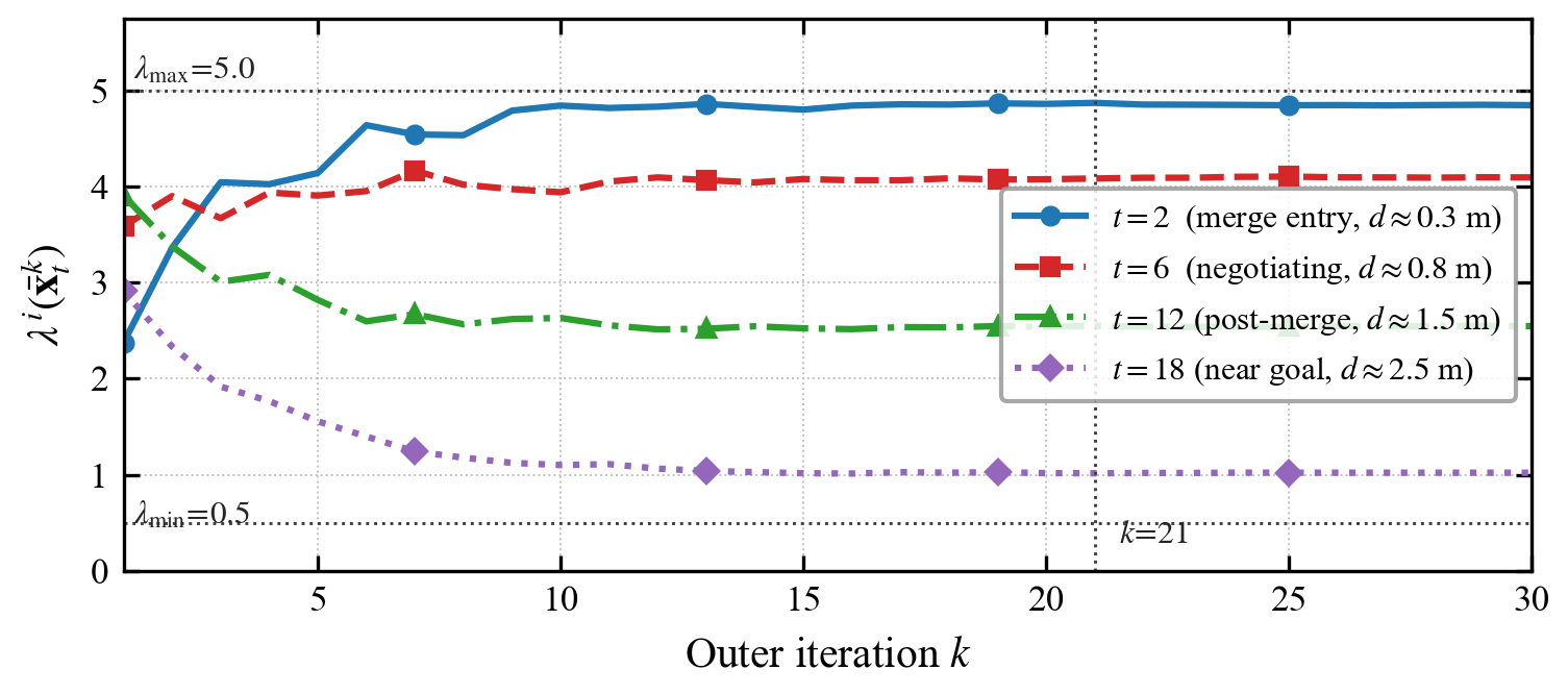
(a) Evolution of across outer iterations.

(b) Per-iteration perturbation across outer iterations.
5.4 Convergence of State-Dependent
To illustrate the behavior of the adaptive regularization, we trace at four representative planning steps (each corresponding to s) in the RM scenario across outer iterations of Algorithm 1. As shown in Fig. 7(a), the converged values range from near the merge zone ( m) to near the goal ( m), confirming that the proposed mechanism assigns stronger regularization in regions of high interaction density while granting greater optimization freedom elsewhere. Fig. 7(b) further shows that the per-iteration perturbation remains bounded and decays rapidly, consistent with Proposition 2.
5.5 Hardware Experiments
To validate our framework in real-world scenarios, we conducted hardware experiments involving two TurtleBot4s and a human participant. Each robot used an Intel RealSense T265 camera111https://www.intelrealsense.com/tracking-camera-t265/ for visual-inertial pose estimation. We evaluated two tasks: (i) position exchange, (ii) trajectory crossing. Agents navigated to private goal positions without accessing others’ objectives. Strategies were trained offline using joystick-collected human demonstrations and deployed online. Results are shown in Fig. 8; video demonstrations and implementation details are in the supplementary material. All computations ran on an Intel NUC (Core i7-1260P). With warm-starting and a maximum of iterations, the average per-step planning time was (28 Hz), satisfying the real-time requirement imposed by .

6 Conclusion
We proposed a forward–inverse dynamic game framework for multi-agent trajectory planning that couples scene-aware cost inference with a KL-regularized game solver. A state-dependent regularization weight automatically adapts the policy distribution to interaction density, with theoretical guarantees on per-iteration well-posedness and the Lipschitz continuity of the adaptive regularization weight, as established in Propositions 1 and 2. Experiments confirm competitive parameter recovery and trajectory accuracy. Two limitations should be noted. First, expert demonstrations are currently obtained from forward simulation rather than naturalistic datasets such as INTERACTION [33]. Second, future work will infer agent intentions directly from raw sensory inputs, toward a fully end-to-end multi-agent interaction framework.
Appendix A Proof of Lemma 1 and Theorem 1
A.1 Dynamic Programming Formulation
For each agent , let denote the joint system state, the control action, its mixed strategy, and the reference policy. Define the -value function as
| (28) |
where is the stage cost and is the system dynamics. Applying the dynamic programming principle yields the Bellman equation
| (29) |
where is the optimal value function, and the KL term penalizes deviations of the current policy from the reference distribution at state . For convenience in the subsequent derivations, we omit the time index and the agent index unless necessary.
A.2 Proof of Lemma 1
Proof.
Step 1: Deriving the optimal density via a variational argument.
To characterize the optimal policy, we introduce the Radon–Nikodym derivative of with respect to the reference measure , defined as
| (30) |
Under this reparametrization, both the expected cost and the KL divergence term can be expressed as integrals with respect to . Thus, the Bellman objective as in Eq. (29) reduces to
| (31) |
subject to the normalization constraint . To enforce this constraint, we introduce a Lagrange multiplier and formulate the associated Lagrangian functional
| (32) |
We now consider a perturbed density of the form , where is an arbitrary variation satisfying . Computing the first-order variation of along this perturbation yields
| (33) |
A necessary condition for optimality is that the first variation vanishes for every admissible perturbation . By the fundamental lemma of the calculus of variations, this requires the integrand to vanish -almost everywhere on , i.e,
| (34) |
Solving this equation for produces the unnormalized Boltzmann form
| (35) |
The remaining constant is determined by enforcing the normalization condition , which yields the unique minimizer
| (36) |
Step 2: Establishing the variational equality.
We proceed to establish the variational equality by relating the objective evaluated at an arbitrary policy to that at the optimal policy . Define the regularized cost functional
| (37) | ||||
The key step is to apply the chain rule for Radon–Nikodym derivatives, , which, upon taking logarithms, gives the decomposition
| (38) |
From the explicit form of given in Eq. (36), we obtain
| (39) |
Substituting this expression into Eq. (37) and denoting the log-partition function by , we have
| (40) |
Since , with equality if and only if -almost surely, taking the infimum over all admissible policies in Eq. (40) establishes the variational equality in Eq. (9) and confirms that is its unique minimizer.
Step 3: Gaussian closure in the linear–quadratic setting.
Finally, we verify that admits a closed-form Gaussian representation in the linear–quadratic case. When is quadratic in , the term forms a Gaussian kernel in . If the reference policy is also Gaussian, then remains Gaussian. Consequently, defined in Eq. (36) is Gaussian, with mean and covariance computable in closed form. This Gaussian closure property underpins the analytical characterization of the feedback Nash equilibrium in Theorem 1. This completes the proof. ∎
A.3 Proof of Theorem 1
Proof.
We proceed by backward induction on , showing that retains a quadratic form at every time step and deriving the explicit recursion for its coefficients.
Base case (). At the terminal time, the value function is prescribed by the terminal cost, , where
| (41) |
This is quadratic, so the claimed structure holds at . In deviation coordinates , the boundary conditions are and , provided .
Induction step. Suppose the quadratic structure persists at time , namely
| (42) |
Since is quadratic by Eq. (5) and the linearized dynamics in Eq. (4) are affine, composing Eq. (42) with the dynamics shows that is quadratic in . By Lemma 1, the Bellman update is
| (43) |
The Gaussian closure property (Step 3 of Lemma 1) ensures that the log-partition function is quadratic in its natural parameters, which depend affinely on . Hence admits the quadratic representation
| (44) |
It remains to obtain the explicit coefficients by expanding the Bellman equation, optimizing over , and matching the coefficients of . Substituting Eq. (29) and the quadratic cost approximation yields
| (45) |
Since each agent uses a Gaussian policy , we write , where . We then evaluate the expectation of each bracketed term.
Evaluating Term (1)
Taking expectations with respect to the Gaussian policy yields
| (46) |
Evaluating Term (2)
The closed-form KL divergence between the two Gaussians gives
| (47) |
Evaluating Term (C)
Substituting Eq. (42) into the next-step value, computing the Gaussian moments, and separating purely state-dependent contributions into the quadratic and linear parts of , we obtain
| (C) | ||||
| (48) |
Aggregating Eqs. (46)–(48) and discarding all terms independent of , the optimization problem reduces to minimizing the following functional
| (49) |
We now determine the optimal policy parameters and via the first-order necessary conditions.
Step 1. First-order condition with respect to
Differentiating Eq. (49) with respect to yields
| (50) |
Setting Eq. (50) equal to zero furnishes the stationarity condition. Since the resulting equation is linear in , the optimal control mean is necessarily affine in the state deviation, motivating the linear feedback ansatz
| (51) |
Substituting for every into the stationarity condition and equating the coefficients of and the constant terms separately recovers the gain Eq. (12a) and the offset Eq. (12b), respectively.
Step 2. First-order condition with respect to
Differentiating Eq. (49) with respect to the covariance matrix gives
| (52) |
Setting the first-order condition and solving for yield the closed-form optimal covariance
| (53) |
Step 3. Backward Riccati recursion for
Substituting the optimal policies and back into Eq. (45) and collecting quadratic and linear terms in , we introduce the closed-loop quantities
| (54) |
with all remaining scalar constants absorbed into . Identifying the resulting expression with the postulated quadratic form in Eq. (44) and matching the quadratic and linear coefficients of directly yields the recursions for and , which coincide with Eqs. (13a) and (13b) in the main text. This completes the proof. ∎
A.4 Proof of Proposition 1
Proof.
We first prove Statement 1) by backward induction on . The terminal condition of the value recursion satisfies
| (55) |
by the positive semidefiniteness of the terminal quadratic approximation.
Suppose that, for some , the induction hypothesis holds:
| (56) |
By Assumption 1 (A4), the coupled linear systems in Eqs. (12a)–(12b) are nonsingular. Hence, the feedback gains are uniquely determined. Substituting these gains into Eq. (13a), each term in the recursion is positive semidefinite: by the local quadratic approximation, since , and by the induction hypothesis. Moreover, Eqs. (14) and (16) imply , while follows from the positive-definiteness condition stated in Proposition 1. Hence, we have Therefore, we get . This completes the backward induction and proves Statement 1).
We next prove Statement 2). For any , Statement 1) implies . Therefore,
| (57) |
Using again and , it follows that
| (58) |
Together with the strong convexity condition , it follows that
| (59) |
Therefore, is uniformly positive definite in and , which proves Statement 2).
For Statement 3), substituting the frozen coefficient into Eq. (11b) and using the definition of gives
| (60) |
Since and , it follows that . Thus, the covariance update is well-defined.
Finally, since the coupled linear system in Eqs. (12a)–(12b) is nonsingular, the feedback gains are unique, and so is the mean . Together with the uniquely defined positive definite covariance , this gives a unique Gaussian policy and thus a unique Gaussian FBNE for the frozen local game. This completes the proof. ∎
A.5 Proof of Proposition 2
Proof.
We prove the Lipschitz continuity of by composing the Lipschitz continuity of , the smooth Gaussian kernel, and the affine transformation defining .
Step 1. ( is -Lipschitz). Let and . By Assumption 1 (A3), the position extraction map is linear and non-expansive. Hence,
| (61) |
For the static obstacle term, the distance function to a non-empty closed set is -Lipschitz [34]. Therefore,
| (62) |
For each interaction-distance term with , the reverse triangle inequality gives
| (63) |
Since the pointwise minimum of finitely many Lipschitz functions remains Lipschitz, is Lipschitz continuous. In particular, we may take
| (64) |
Step 2. ( is -Lipschitz). Since the function is continuously differentiable with bounded derivative on , it is Lipschitz continuous. Together with the -Lipschitz continuity of , this implies
| (65) |
for some constant .
Step 3. ( is -Lipschitz). Since is an affine function of in Eq. (14), the Lipschitz continuity of gives
| (66) |
This completes the proof. ∎
References
- [1] R. C. Gil, D. J. Ornia, K. A. Mustafa, and J. Alonso Mora, “Predictability awareness for efficient and robust multi-agent coordination,” in Proceedings of the 24th International Conference on Autonomous Agents and Multiagent Systems, 2025, pp. 886–894.
- [2] X. Liu, L. Peters, and J. Alonso-Mora, “Learning to play trajectory games against opponents with unknown objectives,” IEEE Robotics and Automation Letters, vol. 8, no. 7, pp. 4139–4146, 2023.
- [3] J. Li, C.-Y. Chiu, L. Peters, S. Sojoudi, C. Tomlin, and D. Fridovich-Keil, “Cost inference for feedback dynamic games from noisy partial state observations and incomplete trajectories,” in Proceedings of the 2023 International Conference on Autonomous Agents and Multiagent Systems, 2023, pp. 1062–1070.
- [4] J. Lidard, H. Hu, A. Hancock, Z. Zhang, A. G. Contreras, V. Modi, J. DeCastro, D. Gopinath, G. Rosman, and N. E. Leonard, “Blending data-driven priors in dynamic games,” in Proceedings of Robotics: Science and Systems (RSS), Delft, Netherlands, Jul. 2024.
- [5] M. Rowold, A. Langmann, B. Lohmann, and J. Betz, “Open-loop and feedback nash trajectories for competitive racing with ilqgames,” in 2024 IEEE 27th International Conference on Intelligent Transportation Systems (ITSC). IEEE, 2024, pp. 1827–1834.
- [6] G. Galati, A. Usai, G. Vignolo, S. Macrì, and A. Rizzo, “A game of social forces: Integrating non-cooperative game theory with social force model for a socially-acceptable mobile robot navigation,” Journal of Intelligent & Robotic Systems, vol. 111, no. 4, p. 110, 2025.
- [7] L. Peters, V. Rubies-Royo, C. J. Tomlin, L. Ferranti, J. Alonso-Mora, C. Stachniss, and D. Fridovich-Keil, “Online and offline learning of player objectives from partial observations in dynamic games,” The International Journal of Robotics Research, vol. 42, no. 10, pp. 917–937, 2023.
- [8] W. Huo, L. Huang, S. Dey, and L. Shi, “Neural-network-based distributed generalized nash equilibrium seeking for uncertain nonlinear multiagent systems,” IEEE Transactions on Control of Network Systems, vol. 11, no. 3, pp. 1323–1334, 2023.
- [9] J. Liu, X. Liao, J.-S. Dong, and A. Mansoori, “Continuous-time distributed generalized nash equilibrium seeking in nonsmooth fuzzy aggregative games,” IEEE Transactions on Control of Network Systems, vol. 11, no. 3, pp. 1262–1274, 2023.
- [10] X. Liao, W. Meng, and X. Li, “Fully distributed primal-dual generalized nash equilibrium seeking algorithm under partial-decision information,” IEEE Transactions on Control of Network Systems, 2025.
- [11] Q. Meng and Q. Ma, “Distributed nash equilibrium seeking for games in uncertain nonlinear systems via adaptive backstepping approach,” IEEE Transactions on Control of Network Systems, vol. 12, no. 1, pp. 1188–1198, 2024.
- [12] E. Çinlar, Probability and Stochastics. Springer, 2011.
- [13] S. Le Cleac’h, M. Schwager, and Z. Manchester, “Lucidgames: Online unscented inverse dynamic games for adaptive trajectory prediction and planning,” IEEE Robotics and Automation Letters, vol. 6, no. 3, pp. 5485–5492, 2021.
- [14] N. Mehr, M. Wang, M. Bhatt, and M. Schwager, “Maximum-entropy multi-agent dynamic games: Forward and inverse solutions,” IEEE Transactions on Robotics, vol. 39, no. 3, pp. 1801–1815, 2023.
- [15] V. S. Donge, B. Lian, F. L. Lewis, and A. Davoudi, “Multiagent graphical games with inverse reinforcement learning,” IEEE Transactions on Control of Network Systems, vol. 10, no. 2, pp. 841–852, 2022.
- [16] H. W. Kuhn and A. W. Tucker, “Nonlinear programming,” in Proceedings of the Second Berkeley Symposium on Mathematical Statistics and Probability. University of California Press, Berkeley and Los Angeles, 1951, pp. 481–492.
- [17] J. F. Fisac, E. Bronstein, E. Stefansson, D. Sadigh, S. S. Sastry, and A. D. Dragan, “Hierarchical game-theoretic planning for autonomous vehicles,” in 2019 International Conference on Robotics and Automation (ICRA). IEEE, 2019, pp. 9590–9596.
- [18] O. So, P. Drews, T. Balch, V. Dimitrov, G. Rosman, and E. A. Theodorou, “Mpogames: Efficient multimodal partially observable dynamic games,” in 2023 IEEE International Conference on Robotics and Automation (ICRA). IEEE, 2023, pp. 3189–3196.
- [19] Y. Sheng, Y. Wang, H. Cheng, H. Zhao, and H. Ding, “Human-like robot action policy through game-theoretic intent inference for human–robot collaboration,” IEEE Transactions on Robotics, vol. 41, pp. 5411–5430, 2025.
- [20] T. Başar and G. J. Olsder, Dynamic noncooperative game theory. SIAM, 1998.
- [21] F. Laine, D. Fridovich-Keil, C.-Y. Chiu, and C. Tomlin, “The computation of approximate generalized feedback nash equilibria,” SIAM Journal on Optimization, vol. 33, no. 1, pp. 294–318, 2023.
- [22] J. Ruiz-Serra, P. Sweeney, and M. S. Harré, “Factorised active inference for strategic multi-agent interactions,” in Proceedings of the 24th International Conference on Autonomous Agents and Multiagent Systems, 2025, pp. 1793–1802.
- [23] C. Awasthi and A. Lamperski, “Inverse differential games with mixed inequality constraints,” in 2020 American Control Conference (ACC), Jul 2020, p. 2182–2187.
- [24] C. Finn, S. Levine, and P. Abbeel, “Guided cost learning: deep inverse optimal control via policy optimization,” in Proceedings of the 33rd International Conference on International Conference on Machine Learning-Volume 48, 2016, pp. 49–58.
- [25] L. Yu, J. Song, and S. Ermon, “Multi-agent adversarial inverse reinforcement learning,” International Conference on Machine Learning, May 2019.
- [26] D. Fridovich-Keil, E. Ratner, L. Peters, A. D. Dragan, and C. J. Tomlin, “Efficient iterative linear-quadratic approximations for nonlinear multi-player general-sum differential games,” in 2020 IEEE International Conference on Robotics and Automation (ICRA), 2020, pp. 1475–1481.
- [27] N. Jeong and D. Lee, “Finite-time analysis of minimax q-learning,” in Reinforcement Learning Conference, 2025.
- [28] C. M. Bishop and N. M. Nasrabadi, Pattern recognition and machine learning. Springer, 2006, vol. 4, no. 4.
- [29] M. Wulfmeier, P. Ondruska, and I. Posner, “Maximum entropy deep inverse reinforcement learning,” arXiv preprint:1507.04888, 2015.
- [30] J. Gao, C. Sun, H. Zhao, Y. Shen, D. Anguelov, C. Li, and C. Schmid, “Vectornet: Encoding hd maps and agent dynamics from vectorized representation,” in Proceedings of the IEEE/CVF Conference on Computer Vision and Pattern Recognition, 2020, pp. 11 525–11 533.
- [31] B. D. Ziebart, A. L. Maas, J. A. Bagnell, A. K. Dey et al., “Maximum entropy inverse reinforcement learning.” in Aaai, vol. 8. Chicago, IL, USA, 2008, pp. 1433–1438.
- [32] J. Lubars, H. Gupta, S. Chinchali, L. Li, A. Raja, R. Srikant, and X. Wu, “Combining reinforcement learning with model predictive control for on-ramp merging,” in 2021 IEEE International Intelligent Transportation Systems Conference (ITSC). IEEE, 2021, pp. 942–947.
- [33] W. Zhan, L. Sun, D. Wang, H. Shi, A. Clausse, M. Naumann, J. Kümmerle, H. Königshof, C. Stiller, A. de La Fortelle, and M. Tomizuka, “INTERACTION dataset: An INternational, Adversarial and Cooperative moTion dataset in interactive driving scenarios with semantic maps,” arXiv preprint arXiv:1910.03088, 2019.
- [34] W. Rudin, Principles of Mathematical Analysis, 3rd ed. McGraw-Hill, 1976.