Bulk-Boundary Correspondence in Semi-Infinite Chains from Sublattice Zeros
Abstract
We provide an alternative derivation of the bulk-boundary correspondence for semi-infinite chains. To describe edge states, we analytically continue the usual Bloch Hamiltonian to complex wave vectors . To start, we note that the zeros of a Bloch wavefunction are related to edge states, at least in systems with nearest-neighbour hoppings. We show that an analytically continued Bloch Hamiltonian with chiral symmetry has exceptional points, where two different states coalesce. These special points are related to the adiabatic protection of edge states. We derive a winding number that counts the number of topological edge states protected by chiral symmetry.
I Introduction
It is a known fact that the Zak phase [18], evaluated in a specific unit cell and gauge, is related to the number of midgap edge states in chiral symmetric, one dimensional, semi-infinite topological insulators [17, 19]. Furthermore, the physical reason for this correspondence is hidden behind a layer of involved mathematics, which is used to derive this correspondence (for example, using -theory [16]). In this paper, we will provide an alternate derivation of the bulk-boundary correspondence for semi-infinite chains with chiral symmetry. The goal of the derivation is to understand the mechanisms behind this result in a physically insightful way, as well as to provide a bulk-boundary correspondence that does not depend on the choice of unit cell and gauge. We relate our results to the Zak phase and its variants.
There are two main insights in the paper that as far as we know have not been previously elucidated. Firstly, we establish that, under certain circumstances, edge states are related to wavefunction zeros of analytically continued Bloch states. Secondly and most importantly, we show that the adiabatic protection of edge states is directly related to the presence of non-diagonalizable (exceptional) points of the analytically continued Bloch Hamiltonian, where two states coalesce. These special points are caused by the presence of chiral symmetry.
The paper is organized as follows. Sec. II covers some prerequisites for the rest of the paper and discuss the analytic continuation of the Bloch Hamiltonian. In Sec. III, we relate states of semi-infinite chains to those of the corresponding infinite chain. In Sec. IV, we derive a winding number that counts (not necessarily adiabatically protected) edge states. In Sec. V, we establish the conditions under which the number of edge states is an adiabatic invariant and provide the appropriate topological invariant. Sec. VI concludes the paper with some closing remarks.
II Analytic Continuation of Bloch Hamiltonian
Our goal is to find edge states of a semi-infinite chain with -site unit cell and hoppings which are -site periodic but which are not necessarily limited to nearest neighbors. Since a semi-infinite chain is essentially a truncated infinite chain plus one or more boundary conditions, we begin our search by briefly looking at the states of the corresponding infinite chain, with Hamiltonian . We will then transition to the semi-infinite chain by first relaxing the normalization condition on eigenstates and then incorporating the appropriate boundary conditions.
Let the sites be labeled by the unit cell index , and the sublattice index , so represents a particle localized on the site of the unit cell. Periodicity implies that is independent of , so we write
| (1) |
where the second equality follows from the Hermiticity of . The matrix and its hermitian conjugate contain the inter-cell hopping parameters.
The Hamiltonian can be viewed as an infinite-dimensional matrix of -dimensional blocks. The blocks along the diagonal contain the matrix ; those along the first subdiagonal below and above contain and , respectively; and so on. In what follows, it will be useful to define , the farthest hopping in terms of unit cells; thus, beyond the subdiagonal above and below, . We also define the hopping range as follows: if only nearest-neighbour hoppings are present, ; if next-nearest-neighbour hoppings are also present, ; etc.
Bloch states are formed via Fourier transformation
| (2) |
where and is the lattice constant. (Note the semicolon on the left and comma on the right, signifying that the first state label is a wave number on the left and a unit cell index on the right. This convention will be followed throughout the paper.) These states obey the following orthonormality condition:
| (3) |
with and being the Dirac and Kronecker deltas, respectively. The -dimensional Bloch Hamiltonian is defined by
| (4) |
giving
| (5) |
Hermiticity of (for real) is guaranteed by (1).
For an infinite chain, states with are unacceptable since they are non-normalizable: they diverge exponentially as for . However, for a semi-infinite or finite chain, such states are not only permitted — they are of great interest. Since they grow exponentially towards the boundary, they are perfect candidates for edge states. To accommodate these states we must replace , so in analogy with (2) and (5) we define
| (6) | ||||
| (7) |
This gives rise to various complications since the analytically continued Bloch Hamiltonian (7), viewed as a function of the complex parameter , is only Hermitian on the unit circle . Thus, we lose many properties normally taken for granted such as orthonormality of eigenstates, diagonalizability by a unitary matrix, etc.
Fortunately, , while not Hermitian, has a related property (with related consequences) known as para-Hermiticity [4, 7]:
| (8) |
(On the unit circle , so we recover the usual Hermiticity.) The Schrödinger equation for is
| (9) |
where is the band index and is an -component eigenvector.
Para-Hermiticity has the following consequences for (9):
-
1.
The energies satisfy
(10) (so is not, in general, real).
-
2.
The Bloch eigenstates satisfy
(11) where are band indices and .
The second property implies that, whenever has a complete basis of eigenstates (which, as we shall see, is not always the case), it can be diagonalized by a para-unitary matrix , that is, one satisfying .
Importantly for the following, is analytic for nonzero and finite, as can be seen from (7). Therefore, there is always a choice of normalization and gauge for which is non-zero and analytic, except for possible branch points [9]; these arise in both and at non-diagonalizable (exceptional) points of [13, 5, 8, 12]. Near an exceptional point, both and exhibit branch-point behaviour with a local dependence of the form , where the order depends on the structure of the Hamiltonian.
III Bulk and boundary states
Energy eigenstates for the infinite chain are easily constructed in terms of the Bloch eigenstates. We define to be the Bloch eigenstate in the unit cell and zero outside; then the eigenstates (ignoring normalizability) are
Given that inter- and intra-band degeneracies are possible, the most general eigenstate of energy is
| (12) |
where are complex coefficients and is the set of values for which the energy is (that is,
).
Consider now a semi-infinite chain (henceforth referred to as the system) with edge on the left and extending to infinity on the right. (The analysis can easily be adapted to a semi-infinite chain extending to infinity on the left.) Let denote the hamiltonian of the system. Any state of the infinite chain corresponds to a state of the system by reduction (dropping the components of the state corresponding to the excised sites); we write
| (13) |
States with are bulk states; states with are edge states; states with grow exponentially and are eliminated by normalization.
Applying to the energy eigenstate (12) will not automatically result in an eigenstate of the system; the coefficients must satisfy certain boundary conditions that depend on the details of the model. Consider the case where one boundary condition is , where is the first site exterior to the chain. Although other boundary conditions may be required (see App. A for a detailed discussion), it will give us important insights, and we shall focus on this specific condition throughout the next sections.
We will assume that, for edge states, the reduction of (12) satisfies the boundary condition with a single nonzero coefficient. In other words, we will assume that the edge states can be obtained from a single analytically continued Bloch state. At first glance, this may seem unlikely; however, we argue in Sec. V that this assumption holds for edge states. Under this assumption, edge states are of the form
| (14) |
for one or more . The boundary condition implies that
| (15) |
where we have defined , the Bloch state amplitude on the sublattice associated with the state (14). Thus, for an edge state of this form the wave function at every -th site along the chain vanishes.
We show in subsection V.3 that the number of (analytically continued) Bloch states satisfying (III) can be adiabatically protected under certain conditions. If these conditions are satisfied, it suffices for a system to be adiabatically connected to one where (III) holds trivially in order for it to have edge states that can be obtained from a single Bloch state.
IV Counting Edge States Satisfying the Boundary Condition
IV.1 Edge States without Branch Cuts
Assuming that edge states are analytically continued Bloch states with a zero in one sublattice, we can construct a winding number that gives the number of edge states satisfying the boundary condition (assumed to be sufficient throughout this section), as follows. If is diagonalizable for nonzero and finite, then can be assumed to be analytic on the same domain [9]. (It was noted at the end of Sec. II that is not always diagonalizable, the implications of which will be explored in detail in subsection V.2.) Let be a bounded domain in . Denote the zeros of lying within and their multiplicities, respectively, by and (). Furthermore, assume that no zeros occur on the boundary . Then the argument principle applied to the function gives
| (16) |
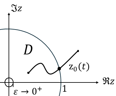
Given that the boundary of the system is on the left, we need only consider states with . Thus, we will restrict to , as illustrated in Fig. 1. The number of edge states coming from the -th band is bounded from above by
| (17) |
where consists of the unit circle (integrated anti-clockwise) and a circle of infinitesimal radius centred at the origin (integrated clockwise). This bound is saturated (that is, gives the exact number of edge states from the -th band) if for all , while if any multiplicities are greater than one (17) will overcount the number of edge states.
Multiplicities greater than one do not occur generically (they require fine tuning of the parameters in the Hamiltonian), and they are unstable against a small perturbation. For example, suppose , so that is a zero of multiplicity 2 at and consider the small perturbation , where . Now, , which has two zeros of multiplicity 1. This argument is easily generalized to zeros of higher order. Thus, while (17) gives the maximum number of edge states, generically it gives the exact number of edge states, and henceforth we will assume this to be true.

We note the similarity between (17) and the previously established sublattice Zak phase [14, 15, 1]. In fact, if we choose a normalization such that (as was done in [1]), then (17) reduces to
| (18) |
where is the projector on the boundary sublattice. This is none other than the Zak-Berry phase of the sublattice (albeit with a different domain of integration). It has already been shown that the sublattice Zak phase is able to correctly predict the number of edge states in certain cases [1, 14, 15]. Note that the chosen normalization makes non-analytic. Since it does not affect the argument of , it will still give the same quantity as (17) in the non-normalized case. To highlight a side point, any choice of gauge and normalization that keeps analytic must be coherent with the argument principle; thus, (17) is invariant under an analytic choice of gauge and normalization.111In practice, however, we may not have control over the gauge, for example in a numeric calculation. To remove the reliance on an analytic gauge, it is possible to compute the difference of for two different boundaries.
Finally, does not depend on the choice of unit cell, since a change of unit cell must be accompanied with the corresponding change of what sublattice amplitude is called “”. In practice, a change of unit cell results in a change of the order of the poles at , but does not affect the multiplicities or positions of the zeros. Therefore, since excludes , remains unchanged.
IV.2 Edge States with Branch Cuts
Of particular interest in what follows will be edge states arising at non-diagonalizable points of in -space. As has been noted in Sec. II, the eigenstates and eigenvalues of can develop root singularities at the non-diagonalizable, exceptional, points [13, 5]. We will only be concerned with exceptional points corresponding to eigenstates and eigenvalues that coalesce [3]. For such states, (17) will return , where is the order of the root singularity [12]. For example, in the case of a square root singularity, which is particularly common (for a concrete example, see App. B), will give half of the total multiplicity of the zeros of . In the presence of exceptional points, the index by itself can only tell us that there are edge states (provided that the boundary condition (III) is sufficient), rather than telling us the maximum number of edge states. Because in that case all edge states have the same branch cut, we can compute the number of Bloch states satisfying (III) with
| (19) |
since each band with an edge state will contribute , and there are such bands coalescing.
V Adiabatic Invariant
Consider the manner in which a continuous change in the Bloch Hamiltonian can affect the number of edge states that satisfy a boundary condition of the form (III). Under a continuous change of the Hamiltonian that does not close the gap (in other words, an adiabatic change), the eigenstates, and thus the coefficients , will also change continuously. We wish to show that the zeros of cannot disappear from the complex plane during this evolution for nonzero and finite (so that , and thererfore , is analytic).
Assume the evolution of the Hamiltonian is parameterized by a parameter , with the original Hamiltonian corresponding to . Then with . Any zero of , denoted , are given by
| (20) |
The function remains analytic throughout the evolution. We can assume that, in the neighbourhood of , .222This assumption is obviously true for zeros of multiplicity 1 since, in the neighbourhood of the zero, . As we have seen, we can easily split a zero of order into zeros of order 1 by a small perturbation. The same argument will apply then and the total multiplicity of zeros is conserved. By the implicit function theorem there exists a unique continuous path given by the solution of the equation
We conclude that the zero does not disappear and follows a smooth path parameterized by .
An adiabatic evolution, by definition, must be invertible. If a zero appeared at some , then in the inverse process, the zero would disappear. Since this process is also continuous, this would contradict our previous statement. Therefore, we arrive at the conclusion that the multiplicity of zeros of cannot be changed adiabatically for nonzero and finite. In other words, in an infinite system, Bloch states satisfying (III) cannot be created or destroyed in this range: they can only shift around in space.
This justifies our focus on Bloch states with : although those states might seem improbable, if some system has such a Bloch state, every system to which it is adiabatically connected also has a Bloch state with that sublattice zero at some value of .
V.1 From Infinite to Semi-Infinite
We have just argued that the zeros of the function cannot be created or destroyed for nonzero and finite. We know that if , then a boundary condition of the form (III) is satisfied. However, for that state to be normalizable, it must have . Nothing prohibits the zeros of to cross the unit circle adiabatically. Therefore, generally, edge states respecting the boundary condition (III) are not adiabatically protected, as is the case in the SSH3 model [1]. A possible path of a zero during an adiabatic evolution, , is shown in Fig. 2.
Before continuing, we must address the fact that, being non-analytic at and , it seems like new edge states can appear and disappear at these points. In our system, a state with is one entirely localized in the first unit cell. An acceptable state of the system can only arise at such a value of when there are no inter-cell hoppings (otherwise (7) will have an “acceptable” state with infinite energy). New edge states can appear and disappear when there are no inter-cell couplings (what might be called the “-merized” limit), for this reason we shall restrict the adiabatic evolutions that we consider to those that avoid this limit.
It is important to understand how adiabatic protection fits in our picture. If the of an edge state crosses the unit circle, , it will go from normalizable to non-normalizable and thus disappear from the semi-infinite system. For adiabatically protected states, we require that a gap close when this happens. This is true if the edge state belongs to multiple bands at once or, in other words, if with and some . This can happen at exceptional points of the analytically continued Bloch Hamiltonian. Those exceptional points correspond to two (or more) states coalescing at , making non-diagonalizable at that point.333In the literature there exists a number of definitions of the term exceptional point. We are only concerned with this specific type. We will refer to the states that coalesce at an exceptional point as exceptional states. When such a state crosses , there must be a band crossing, since this state has a real , meaning that for some , .
V.2 Exceptional points
Through what has been said above, we can see that the edge states that satisfy the boundary condition (III) and arise at exceptional points are adiabatically protected (provided the edge state remains exceptional throughout the adiabatic evolution, this will be addressed in subsection V.3). It is useful to understand how to count the number of exceptional points.
Consider equation (11). When two different states coalesce at an exceptional point,
| (21) |
with . This phenomenon is called self-orthogonality [13]. Note that we assume a normalization such that does not have poles; otherwise, we may choose
which will not satisfy (21).
The para-Hermitian norm
| (22) |
is analytic up to branch cuts [5, 8, 9]. We can use this property to count its zeros in . Each of them will correspond to a self-orthogonal exceptional point. To do so, we will again use the argument principle:
| (23) |
where does not count the total number of exceptional points, but rather times the number of exceptional states in band , where is the number of states coalescing.444As has been mentioned previously, if states coalesce, the branch cut will be caused by a root of order [12]. The total number of exceptional points is thus given by
| (24) |
Interestingly, each can be written in terms of the analytically continued Berry connection
| (25) |
Let be a circle of radius centered at . Then
| (26) |
V.2.1 Connection to Topology
We can organize the eigenstates of into a matrix and count the number of exceptional points in this way. We define
| (27) |
Since we chose a gauge and normalization such that is analytic (up to branch cuts) and nonzero, is itself analytic up to branch cuts. Furthermore, only when two states coalesce, thus
| # e.p. | ||||
| (28) |
where in the second line we have used Jacobi’s formula. Here, a factor appears in the numerator because each exceptional point will contribute to this integral. Note that we assume to be invertible on . is invertible when is diagonalizable, so we will also assume that is diagonalizable on the integration path. (28) can be interpreted in terms of homotopy between and .
, evaluated along a loop, is a mapping (again, we assume that is diagonalizable on that loop). Let us define the winding
| (29) |
This winding represents a homotopy class of [5]. In terms of , we can rewrite (28) as
| (30) |
If , it means that there is a discontinuity in the mappings , since two mappings with different have a different homotopy. This discontinuity occurs because, at the exceptional point, is no longer invertible and the mapping is not defined.
Although our initial investigation of edge states relied on the validity of the boundary condition (III), allowing us to emphasize the importance of zeros of the wave function, we have now gained the insight that the number of exceptional points of an analytically continued Bloch Hamiltonian is adiabatically protected. Therefore, if one is given a boundary condition (not necessarily (III)) and wishes to construct an adiabatically protected state, one must do so by combining exceptional states. The number of exceptional points is thus directly related to the number of edge states.
V.3 Chiral Symmetry
Although we have established that edge states arising at exceptional points are adiabatically protected, we have not yet explained under which circumstances exceptional points do appear. One such circumstance arises if the Hamiltonian has chiral symmetry, that is, if a constant, unitary, Hermitian matrix exists which anticommutes with the -dimensional Bloch Hamiltonian: . With a change of basis, and can be brought to the form
| (31) | ||||
| (32) |
Chiral symmetry divides the system into sublattices of positive and negative chirality, which we will refer to as sublattice and , respectively. The energy spectrum is symmetric; in the above basis, eigenstates of equal and opposite nonzero energy are given by
| (33) |
with and nonzero.
If either or is zero, the two states are identical (up to a sign), and the state must have zero energy. This is trivially guaranteed to occur for all if is odd-dimensional. Since such a zero-mode is unrelated to the considerations in this paper we will assume henceforth that is even and is a square matrix.
With even, while zero-modes are not required, it is entirely possible that at isolated values of either or is zero, again giving a zero-mode. Such values of and the associated zero-modes are the exceptional points and exceptional states referred to in the previous subsections.
Note that in the case of chiral symmetry, (states always coalesce in pairs). These exceptional states always have half of their components fixed to zero; therefore they always satisfy a boundary condition of the form (III). However, as has been discussed, the number of exceptional states can give us the number of adiabatically protected edge states for boundary conditions of other forms as well.
Equation (31) implies that
| (34) | ||||
| (35) |
If , then . The boundary of a semi-infinite system has to fall either in subspace or in subspace . We know that when , has an exceptional point. When this happens, we also satisfy a boundary condition; therefore, chiral symmetry protected zero energy edge states arise at the exceptional points of , at least when the hoppings going through the boundary are to the nearest neighbour.
The matrix from (27) is given by
| (36) |
We wish to find the points associated either with or with . Since diagonalizes the Hamiltonian, where is the -th sublattice. (which we will hereafter simplify to for ease of reading) is the state with opposite energy associated with ; therefore we can write
| (37) | ||||
| (38) |
where (with 1 in the -th position) is a -dimensional vector. If , (37) and (38) tell us . This condition is sufficient for the existence of an edge state at an exceptional point. is analytic up to branch cuts, we can therefore count the exceptional states with using the argument principle,
| (39) |
Just as before, this expression can be understood in terms of the homotopy classes. Note that because of the square root, .
To compute (39), we need to fix a gauge and a normalization that makes analytic up to branch cuts. Often, we do not have control on the gauge of the eigenstates when performing numerical calculations. A more computable quantity is
| (40) |
should not require an analytic choice of gauge, nor does it require to have a normalization that avoids poles, since any normalization and gauge in will be cancelled by . It can be shown that [11], where are the normalized (para-unitary) matrices , such that
| (41) |
By defining , we can write
| (42) |
which is the usual chiral winding number [6], although integrated on a slightly different domain (usually the integral is performed on ). This is also equal to the sum of Zak-Berry phases of all of the bands (evaluated around ). Note that is in the flat band limit.
The winding number does not tell us how many edge states there are, however it tells us the difference between the number of exceptional states with and in , which is an adiabatic invariant and is related to the number of edge states. Usually, the chiral winding number only predicts the correct number of edge states when a specific unit cell was chosen, this result is thus not surprising.
For the same reasons as discussed at the end of subsection IV.1, the winding numbers presented here do not depend on the choice of unit cell.
We have, in this section, shown the existence of chiral symmetry protected zero energy states in the Bloch Hamiltonian. Those states can be used to construct edge states of a semi-infinite system. In particular, if the boundary condition (III) is sufficient, (39) directly counts the number of edge states of the semi-infinite chain.
V.4 Moving Away from Nearest-Neighbour Hoppings Across the Boundary
As discussed in Sec. III, the boundary condition
| (43) |
is only sufficient if the only hoppings crossing the boundary (in the corresponding infinite system) are to the nearest neighbour. In general, for hopping range there will be up to boundary conditions, and (43) is not necessarily sufficient. We will now generalize the treatment above to such systems.
By studying the zeros of the Bloch wavefunction we have gained the important insight that chiral symmetry leads to adiabatically protected states with or , due to the presence of exceptional points. When boundary condition (III) is sufficient, it so happens that such exceptional states are also edge states. It is reasonable to assume that the existence of these exceptional points in systems with chiral symmetry is the only mechanism which causes adiabatically protected states. Counting the number of Bloch states with or is not necessarily sufficient to count the number of states fully satisfying the boundary condition, but it allows one to count the dimension of the set of states which can be used to construct an adiabatically protected edge state. Additionally, through the and conditions, the exceptional states of chiral symmetric Hamiltonians start with at least half of the boundary conditions already being satisfied. Knowing the number of remaining boundary conditions and the dimension of the and subspaces, one can exactly predict the number of edge states of a semi-infinite system.
In this view, one should interpret the windings as counting the dimensions of the spaces of adiabatically protected Bloch states which can be used to construct a semi-infinite edge state. If there are boundary conditions left to satisfy in the or subspaces, the number of edge states from either subspace is
| (44) |
Whenever the dimension of the space of available exceptional points changes, the gap closes and the number of edge states changes. A more detailed analysis of the possible boundary conditions is presented in App. A.
VI Conclusion
We have provided a physically insightful derivation of the bulk-boundary correspondence in semi-infinite generalized SSH chains with minimal use of highbrow mathematics. The important insights are that adiabatically protected edge states satisfy a boundary condition that forces every -th site to be zero and occur at the exceptional points of the analytically continued Bloch Hamiltonian. This insight also allows for a new interpretation of the well-established winding number for chirally symmetric Hamiltonians.
Note that, although one can use the bulk Bloch Hamiltonian to determine the number of edge states in a semi-infinite chain, it is perhaps an overstatement to describe this as a bulk-boundary correspondence, in that the bulk part of this relationship is not fully independent of the boundary. For instance, for the basic SSH model there are two possible unit cells ( or ), and the bulk calculation – the Zak phase – will give different results for the two choices. The correct choice of unit cell is determined by the precise edge of the chain.
Acknowledgements.
We thank Hichem Eleuch, Michael Hilke and Andrew Mckenna for useful conversations. This work was supported in part by the Natural Science and Engineering Research Council of Canada and by the Fonds de Recherche Nature et Technologies du Québec via the INTRIQ strategic cluster grant.Appendix A Boundary Conditions of Semi-Infinite Chains
Much of what has been said previously relies on the assumption that the boundary condition is sufficient for a semi-infinite system. Let us examine in more detail the possible boundary conditions of a semi-infinite chain in order to understand the edge states that can be described by our construction.
Let be the Hamiltonian of an infinite chain; suppose we are interested in the semi-infinite chain obtained by excising all sites to the left of a given site. It is useful to write as a matrix of infinite-dimensional matrices:
| (45) |
Here is the Hamiltonian of the excised semi-infinite chain, is the Hamiltonian of the system, and represent the coupling between the two semi-infinite chains. The matrices and are of course Hermitian; the form of will be discussed presently.
We are looking for eigenstates of the infinite chain which give eigenstates of the system upon reduction. The Schrödinger equation for the infinite system can be written in block-diagonal form:
| (46) |
where is the wave function of the infinite chain and and are the parts corresponding to the excised semi-infinite chain and the system, respectively. From the second component of this equation, we see that is a solution of the system’s Schrödinger equation if and only if .
For a system with hopping range (defined in Sec. II), is of the form
where is an -dimensional upper triangular matrix:
| (47) |
Labeling the matrix elements by their position relative to the top right corner is useful since then is the hopping linking the site of the semi-infinite system to the excised site. Of course, if not all hoppings up to range are present, some matrix elements within the triangle will be zero.
Under what circumstances is ? Letting be the lower components of (corresponding to the sites closest to the boundary), we see that if and only if
This equation encapsulates the boundary conditions on the semi-infinite system. Thus, the number of boundary conditions is given by . For instance, if all diagonal elements are nonzero then and an eigenstate of the infinite chain truncates to an eigenstate of the semi-infinite chain if and only if .
For each line of zeros in , there is one less boundary condition. Let’s write the number of boundary conditions as . Note that may depend not only on the length of the hoppings in a system, but also on the specific boundary under consideration.
We are now in a position to state under which circumstances our boundary condition is sufficient. This is true if only the rightmost column of is nonzero. The most natural way for this to occur is if (corresponding to a chain with only nearest-neighbour hoppings). But it is also possible for if the only hoppings that link sites of the system to excised sites land on the first excised site, .
Knowing that states of the analytically continued Bloch Hamiltonian which arise at exceptional points and have chiral symmetry are adiabatically protected, it is reasonable to assume that any topological edge state of a semi-infinite chain must arise as a linear combination of those exceptional states. Consider a chain with at least nearest-neighbour hoppings and chiral symmetry. Its chiral symmetry operator is necessarily
| (48) |
Edge states protected by chiral symmetry must therefore have the form
| (49) |
One of the states above always satisfies at least half of the conditions, therefore in reality, there are at most conditions left to satisfy for the exceptional states. Let’s define as the number of boundary conditions left to satisfy in the exceptional state subspace. If a system has exceptional states, then in the space of exceptional states, the set of boundary conditions leads to linear equations with variables, which has independent solution. If a system has less exceptional points than , it cannot have any adiabatically protected edge states.
Appendix B Example: extended SSH model
We will illustrate our construction through a generalization of the SSH model that has already been studied in [10]. Consider an extension of the SSH model shown in Fig. 3, with real hopping parameters and with range . This model has analytically continued Bloch Hamiltonian
| (50) |
which is non-diagonalizable when or . Its eigenstates, in a gauge and normalization where they are analytic up to branch cuts and non-vanishing, are given by
| (51) |
and its energies are
| (52) |
In accordance with (10) and (11)) and . Furthermore, the two eigenstates coalesce at the non-diagonalizable points of at which .

Consider the corresponding semi-infinite chain. There are 2 possible boundaries for a chain with a boundary on the left:
-
1.
The first site is an element of sublattice .
-
2.
The first site is an element of sublattice .
According to the treatment of App. A, if the first site of the system is an -site, the boundary condition is that the first and third site outside the chain must be zero, a condition which is naturally fulfilled if . If the first site is a -site, the first and second site outside the chain must be zero. If we want to build an adiabatically protected state that fulfills this condition, we need either two states with , or two states with in . The amplitude of the -site can be obtained from that of the site by replacing with , if has two zeros in , has none and vice versa. Since the amplitude of is the square root of a degree 2 polynomial, boundary 1 admits between 0 and 2 adiabatically protected edge states, whereas boundary 2 only admits between 0 and 1.
We can compute the number of exceptional states with either or using (17). Alternatively, we can write down (27) and then compute (39). Here,
| (53) |
from which we deduce that
| (54) |
and
| (55) |
and simply give the components of the wavefunction; therefore, the two approaches are exactly the same. The usual Zak phase is given by the difference of and windings.
The number of exceptional states with or , in is given by, respectively,
| (56) |
and
| (57) |
It varies between 0 and 2 depending on the parameters and . Their nature also varies from purely exponential () to oscillating exponential (). The phase diagram describing the number of exceptional states with is shown in Fig. 4.

Let us focus on the boundary given by case 1. We can compare our approach with using the Zak phase. The Zak phase in this model [2] is given by
This integral can be evaluated by looking at Fig. 4. has a pole of order at which contributes to the integral. This expression is related to the number of zeros of the -site in , which equals . In particular, . Since we’re considering the boundary given by case 1, the number of edge states is actually equal to the number of zeros of , which is , therefore, for this choice of unit cell,
which is the correct number of adiabatically protected edge states. However, contrary to the Zak phase, our expression is independent of the choice of unit cell. Choosing another unit cell is equivalent to , , and , . The new value of is
which counts , thus . However, the new value of is
which counts , and is still the correct number of edge states.
Finally, this model can have two adiabatically protected zero-energy edge states at the same time. Chiral symmetry allows those states to shift from zero energy, but they do not because those states are fixed at exceptional points, which in turn must have zero energy. This illustrates that the adiabatic protection of edge states is not due to chiral symmetry forcing them to be fixed at zero energy, but rather from them occurring at an exceptional point of .
References
- [1] (2022) Bulk-edge correspondence in the trimer su-schrieffer-heeger model. Phys. Rev. B 106, pp. 085109. External Links: Document Cited by: §IV.1, §IV.1, §V.1.
- [2] (2016) A short course on topological insulators. Springer. External Links: Document Cited by: Appendix B.
- [3] (2020) Non-hermitian physics. Advances in Physics 69 (3), pp. 249–435. External Links: Document Cited by: §IV.2.
- [4] (2023) On the rellich eigendecomposition of para-hermitian matrices and the sign characteristics of *-palindromic matrix polynomials. Linear Algebra and its Applications 664, pp. 1–27. External Links: Document Cited by: §II.
- [5] (2021) Exceptional topology of non-hermitian systems. Rev. Mod. Phys. 93, pp. 015005. External Links: Document Cited by: §II, §IV.2, §V.2.1, §V.2.
- [6] (2016) Classification of topological quantum matter with symmetries. Rev. Mod. Phys. 88, pp. 035005. External Links: Document Cited by: §V.3.
- [7] (2024) Para-hermitian rational matrices. SIAM J. Matrix Anal. Appl. 45 (4), pp. 2339–2359. External Links: Document Cited by: §II.
- [8] (2012) Physics of exceptional points. J. Phys. A: Math. Theor. 45, pp. 444016. External Links: Document Cited by: §II, §V.2.
- [9] (1966) Perturbation theory for linear operators. Springer. Cited by: §II, §IV.1, §V.2.
- [10] (2019) Extended ssh model: non-local couplings and non-monotonous edge states. Physics 1 (1), pp. 2–16. External Links: Document Cited by: Appendix B.
- [11] (2021) Real-space representation of the winding number for a one-dimensional chiral-symmetric topological insulator. Phys. Rev. B 103, pp. 224208. External Links: Document Cited by: §V.3.
- [12] (2021) Symmetry and higher-order exceptional points. Phys. Rev. Lett. 127, pp. 186601. External Links: Document Cited by: §II, §IV.2, footnote 4.
- [13] (2011) Non-hermitian quantum mechanics. Cambridge University Press. Cited by: §II, §IV.2, §V.2.
- [14] (2020) Surface charge theorem and topological constraints for edge states: analytical study of one-dimensional nearest-neighbor tight-binding models. Phys. Rev. B 101, pp. 165304. External Links: Document Cited by: §IV.1, §IV.1.
- [15] (2020) Topological invariants to characterize universality of boundary charge in one-dimensional insulators beyond symmetry constraints. Phys. Rev. B 101, pp. 161106. External Links: Document Cited by: §IV.1, §IV.1.
- [16] (2016) Bulk and boundary invariants for complex topological insulators: from k-theory to physics. Springer, Cham. External Links: Document Cited by: §I.
- [17] (2010-06) Topological insulators and superconductors: tenfold way and dimensional hierarchy. New Journal of Physics 12 (6), pp. 065010. External Links: ISSN 1367-2630, Link, Document Cited by: §I.
- [18] (1989-06) Berry’s phase for energy bands in solids. Phys. Rev. Lett. 62, pp. 2747–2750. External Links: Document, Link Cited by: §I.
- [19] (2024) Proof of bulk-edge correspondence for band topology by toeplitz algebra. J. Phys. A: Math. Theor. 57, pp. 465203. External Links: Document Cited by: §I.