Classification of minimal models producing , and masses at one-loop level
Abstract
The Standard Model neither provides a dynamical explanation for the quark and lepton mass hierarchies, nor a rationale for why all of these masses save that of the top quark are suppressed compared to the electroweak scale. Motivated by this, we explore the alternative radiative mass generation hypothesis, specialising to the generation of the , and masses at one-loop level. A classification of all minimal models that use exotic scalars and exotic fermions only is presented, resulting in possibilities featuring four exotic multiplets. As a bonus, some of the models produce a one-loop neutrino Dirac mass if a right-handed neutrino field is included, and some feature WIMP-like dark matter candidates. By way of example, we analyse the phenomenology of a benchmark model chosen from the set of candidates and find that it is capable of exactly replicating the predicted Standard Model Yukawa couplings within the permitted parameter space.
1 Introduction
Apart from the top quark, quarks and leptons have masses that are hierarchically suppressed compared to the electroweak scale. Despite the technical naturalness of the Standard Model (SM) tree-level masses, the hierarchical distribution of the suppressed fermion masses has no dynamical origin in the SM. Because it can explain such a pattern, radiative mass generation for all charged fermions except the top quark is a compelling alternative to standard tree-level mass generation.111The extremely suppressed neutrino mass scale is an egregious and very important special case, but we concentrate on the charged fermions in this paper. The fact that masses arise at loop level accounts for the generic fact of suppression. The hierarchy can then arise from masses that are radiatively generated at sequentially higher loop orders, a possibility that has been studied extensively Weinberg (1972); Balakrishna et al. (1988); Babu and Ma (1989); He et al. (1990); Ma (1990); Dobrescu and Fox (2008); Ma (2014); Cárcamo Hernández et al. (2017); Arbeláez et al. (2020); Weinberg (2020); Baker et al. (2021b); Mohanta and Patel (2022); Bonilla et al. (2023); Jana et al. (2025); Mohanta and Patel (2026); Fraser and Ma (2014); Baker et al. (2021a); Stockdale and Volkas (2025).222Radiative mass generation is not the unique possibility. For example, there is a large literature on using family symmetries and/or seesaw suppression; some representative papers are Froggatt and Nielsen (1979); Davidson and Wali (1987); Rajpoot (1987); Davidson and Wali (1988); Davidson et al. (1990, 1994); Hall and Murayama (1995); Pomarol and Tommasini (1996); Davidson et al. (1999); King and Ross (2001); Carrasco-Martinez and Hall (2026).
Any radiative model of course produces a panoply of testable beyond-SM (BSM) phenomenology. This includes BSM contributions to electroweak precision observables, collider constraints on the direct production of exotic particles, and, for some models, also dark matter candidates. Of particular note is that the SM predicts the relationship , where is the SM vacuum expectation value (VEV), between fermion masses and associated Yukawa couplings. Models which modify how a fermion obtains its mass may also produce a corresponding modification to that fermion’s Yukawa coupling, thus altering the mass-Yukawa relationship. Historically, modified Yukawa coupling constants have not been much analysed. They are, however, becoming increasingly important as the measurements of Higgs decay rates to fermions improve in precision. Multi-family radiative models are also expected to feature flavour-changing Higgs-fermion couplings, which will be subject to strict phenomenological constraints for the lower families.
One-loop radiative masses are well-motivated for the and quarks and the lepton, since their masses are roughly a factor of below the electroweak scale . In a recent work Stockdale and Volkas (2025) we analysed a specific model generating the masses at one-loop level, as well as a one-loop Dirac mass for a single neutrino species. In this paper we generalise our previous effort by classifying all minimal models that generate one-loop effective Yukawas for using only additional scalars and vector-like fermions. We expect some of these will be able to form the basis of a complete model that treats all SM fermions at sequentially higher loop orders.
In Section 2 we review the relevant background, describe the method by which we conducted the model classification, and present a catalogue of all possible minimal models. We examine the theoretical structure and phenomenology of a benchmark model chosen from this catalogue in Section 3. We summarise and finish with some concluding remarks in Section 4.
2 Model classification
We work in the framework formulated in Baker et al. (2021a) and further developed in Stockdale and Volkas (2025). In Section 2.1 we briefly introduce the notation we adopt, before outlining the structure of this framework in Section 2.2. In Section 2.3 we classify all minimal models within this framework that generate one-loop masses for all three of , , and simultaneously.
2.1 Notation
Let be an arbitrary SM fermion, with right-handed component and left-handed component contained in the doublet . In our analysis we will consider . Since we will generate a Higgs Yukawa coupling for at one loop, it is useful to adopt the notation defined in Figure 1, where the are exotic fields which may be scalars or fermions. The exotic couples to both and , to both and , and to both and .
2.2 Model-building framework
In the framework formulated in Baker et al. (2021a), a one-loop mass for a given SM fermion is generated by introducing only new scalars and fermions, and with no modifications to the gauge structure of the theory and only a single Higgs doublet. With these stipulations there are two possible topologies for the one-loop Yukawa diagrams before electroweak symmetry breaking (EWSB), as shown in Figure 2. Class One diagrams feature two exotic scalars which couple to the Higgs, and one exotic fermion, whereas Class Two diagrams feature two exotic fermions which couple to the Higgs, and one exotic scalar.
For a given diagram to exist, the Lagrangian must at a minimum contain the terms corresponding to vertices in the given diagram. Thus
| (1) |
for Class One and Two diagrams respectively, where we have taken to be the lower component of . If it is the upper component, instances of must be replaced with . If the exotic has an or subscript, then it is a fermion; otherwise it is a scalar.
Lorentz- and gauge-invariance of these couplings restrict the quantum numbers of the exotics to those given in Table 1. Additional symmetries may exist and additional terms may be permitted, though these will be model-dependent. Generally these Lagrangians will admit symmetries that are broken only softly by the exotic fermion Dirac mass terms or the scalar trilinear term. We demand our models possess at least one such symmetry that forbids the tree level (or ) Yukawa term, so that the mass has its lowest order contribution at one-loop level.333This is why must not include a term, since no such symmetry could then exist.
| Field | Spin | ||||||
|---|---|---|---|---|---|---|---|
| LI | QI | QII | QIII | ||||
2.3 Minimal models
We wish to construct models that generate one-loop Yukawas for the and simultaneously, and to do so with the fewest new degrees of freedom required. In accordance with this aim, the smallest possible number of exotic fields should be introduced. This is accomplished by identifying some exotics in effective Yukawa diagrams for different SM fermions as the same fields (e.g. ). At least three exotics are obviously required, however it is impossible to produce a combined model for in this framework that introduces only three exotic fields (see Appendix A). Thus we must instead consider the next-most minimal option, those containing four new fields.
To completely classify this set of models, we first generated the set of all possible identifications that can be made between the for , such that there are four total exotic fields. This is equivalent to listing all possible ways that the new fields may interact with the Higgs and the relevant SM fermions. We then discarded any set of identifications possessing any of the following properties:
-
•
Inconsistent spins. For example, requiring and simultaneously.
-
•
No possible hypercharge assignments. Identifications between the different produce a set of simultaneous equations for in accordance with Table 1, for which there sometimes exist no solutions. A simple example of this is requiring and simultaneously.
-
•
Inconsistent groupings. For example, requiring and simultaneously.
-
•
Incapability of forbidding all relevant tree level Yukawa terms. For example, suppose and are both fermions. Then under some arbitrary symmetry. Assuming that does not transform under this symmetry to avoid complications with the other SM Yukawas, the coupling enforces that under said symmetry. Thus it would be impossible to forbid the Yukawa term.
The result of this process is a total of 25 models, which are presented in Table LABEL:tab:minimal_models. We provide the spin and quantum numbers for each of the four new fields, and their correspondences to fields in the one-loop Yukawa diagrams. The exotic hypercharge assignments are fixed for all models, though the and charges are not. In general there are multiple possible patterns for the assignments, so for conciseness we give the assignments with the fewest overall degrees of freedom. We provide the possible assignments in terms of Dynkin labels.
These 25 models may be broadly divided into three separate groups, reflected in our naming convention: pure Class One (CO#) models, pure Class Two (CT#) models, and hybrid (H#) models, in which there will exist both Class One and Class Two topology diagrams. Hybrid models are of particular interest since they have not been studied in this framework previously. We analyse one of these, the H2 model, in greater detail in Section 3 to investigate the generic features these hybrid models may possess.
There are two special “groups” of models, namely CO1a-d and CO2a-d, that will constitute different models in general, but may produce the same model depending on the chosen charges. The key point is that these contain a scalar with zero hypercharge, which we may denote as . If charges are assigned such that is sterile, whenever the Lagrangian contains a term it must also contain , thus the different identifications defining these models would not lead to different structures.
The models CT1, CT3, CO1a-d, CO3, and CO4 are capable of generating a one-loop Dirac Yukawa for a neutrino without any modification to the exotic field content, if a right-handed neutrino is included in the theory. In fact, the model in Stockdale and Volkas (2025) is one such realisation of the CO1a-d models, though it does not explore additional features resulting from the neutrino.
| Name | Exotics | Spin | |||||||||||||||||||||||
|---|---|---|---|---|---|---|---|---|---|---|---|---|---|---|---|---|---|---|---|---|---|---|---|---|---|
| H1 |
|
|
|
|
|
||||||||||||||||||||
| H2 |
|
|
|
|
|
||||||||||||||||||||
| H3 |
|
|
|
|
|
||||||||||||||||||||
| H4 |
|
|
|
|
|
||||||||||||||||||||
| H5 |
|
|
|
|
|
||||||||||||||||||||
| H6 |
|
|
|
|
|
||||||||||||||||||||
| H7 |
|
|
|
|
|
||||||||||||||||||||
| H8 |
|
|
|
|
|
||||||||||||||||||||
| CO1a |
|
|
|
|
|
||||||||||||||||||||
| CO1b |
|
|
|
|
|
||||||||||||||||||||
| CO1c |
|
|
|
|
|
||||||||||||||||||||
| CO1d |
|
|
|
|
|
||||||||||||||||||||
| CO2a |
|
|
|
|
|
||||||||||||||||||||
| CO2b |
|
|
|
|
|
||||||||||||||||||||
| CO2c |
|
|
|
|
|
||||||||||||||||||||
| CO2d |
|
|
|
|
|
||||||||||||||||||||
| CO3 |
|
|
|
|
|
||||||||||||||||||||
| CO4 |
|
|
|
|
|
||||||||||||||||||||
| CO5 |
|
|
|
|
|
||||||||||||||||||||
| CO6 |
|
|
|
|
|
||||||||||||||||||||
| CO7 |
|
|
|
|
|
||||||||||||||||||||
| CO8 |
|
|
|
|
|
||||||||||||||||||||
| CT1 |
|
|
|
|
|
||||||||||||||||||||
| CT2 |
|
|
|
|
|
||||||||||||||||||||
| CT3 |
|
|
|
|
|
3 The H2 model
To see in detail how one of these models works, we choose to examine the H2 case. This provides a contrasting benchmark model to the one we analysed in Ref. Stockdale and Volkas (2025).
3.1 Model structure
To simplify the notation, we denote , as the vectorlike fermions and , as the complex scalars in this model. The defining set of identifications requires our Lagrangian to contain
| (2) |
The quantum numbers of the relevant fields are given in Table 3, choosing the simplest possible set of assignments. This Lagrangian possesses three accidental symmetries: extended lepton and baryon numbers, and exotic parity . It also admits three symmetries that are broken only softly: , , and . These are highly important because forbids tree-level Yukawa coupling terms for , and , thus banishing the generation of tree-level masses for all three relevant species, while forbids and tree-level masses, and forbids a tree-level mass. We choose to impose all three on the dimension-four terms in the theory, but permit the soft-breaking terms that are required for loop-level mass generation. We do not consider any additional terms coupling the exotics to the lighter fermions, so as to remain agnostic to the physics of a complete model treating all three generations.
To avoid bounds on coloured relics, one may include violating terms in the Lagrangian, which will necessarily break the extended lepton and baryon number symmetries to the combination . These violating terms, such as and , will induce mixing between the exotic and SM fermions. This will not reintroduce tree level masses corresponding to or , though it will extend the number of parameters in the theory and alter the mixing behaviour in a way highly specific to this particular model. It would also lead to a violation of unitarity in the CKM sub-matrix, and to proton decay. Alternatively, if the remains unbroken, the stable coloured relics may be inflated away, given that we expect the exotic masses to be TeV. In what follows we only consider mixing between the exotics, since this generalises more simply across the catalogue, corresponding either to an unbroken or small violating terms.
In the absence of violating terms, the only additional terms that must be included are those in the scalar potential, which takes the form
| (3) |
After EWSB, the scalar masses will be given by
| (4) |
The values of other new parameters in the potential, excluding , have no impact on the constraints we consider (at lowest order). We assume that neither nor obtain a VEV.
3.2 Radiative masses and Yukawa couplings
The exotic mixing behaviour is the same as in the standard single class models in Baker et al. (2021a). After EWSB, the trilinear coupling will cause to mix with the lower component of with angle , and the term will cause to mix with the lower component of with angles and . The relevant mass terms may be written
| (5) |
Defining the mass eigenstates as
| (6) |
the resultant mass eigenvalues are
| (7) |
We also obtain the relationships
| (8) |
The one-loop mass diagrams for are as shown in Figure 3, and contributions from each diagram will differ only by various vertex factors. Specifically, the masses at one-loop are
| (9) |
where we have defined
| (10) |
To calculate the effective Yukawa couplings, it is also helpful to define
| (11) |
The expressions for and correspond to the form that effective Yukawa couplings have in pure Class One and Class Two models respectively, in the limit that the Higgs boson four-momentum .
As in all hybrid models, both the exotic fermions and scalars couple to the SM Higgs. The result is that the one-loop effective Yukawas for all relevant SM fermions will have contributions from both topologies in Figure 4, regardless of which topology a particular fermion’s Yukawa diagram was before EWSB. The full expressions are remarkably unwieldy, so while we use them to produce our plots, here we only provide the expressions in certain limits. For and , the charm quark effective Yukawa coupling is given by
| (12) |
The and effective Yukawas will differ slightly due to their original topologies being of a different class. For and , the Yukawa coupling is
| (13) |
The quark effective Yukawa will have the same form, and can be written as
| (14) |
These effective couplings possess a critical difference to those seen in pure models. In the latter, one finds that for all values of the model parameters, with equality approximately recovered as the scale of new physics is increased. However, analysis of the above expressions reveals that hybrid models should be able to produce greater than, equal to, and less than in certain regions of parameter space, and indeed we find this to be the case in Section 3.3. This difference stems from the fact that both types of topologies contribute to the effective Yukawa couplings in hybrid models, and these differing contributions can partially offset one another, whereas pure models will have contributions from only one type of topology. We may thus conclude that the predicted SM relationship can be replicated in radiative mass models, albeit this may come at the cost of significant tuning of the model parameters.
3.3 Phenomenology
We examined several theoretical and experimental constraints on the H2 model, to see what the typical limitations on hybrid models in the catalogue may be. For simplicity we set the exotic fermion and scalar mass scales to be equal, .
The first theoretical constraint we consider is unitarity. The expressions for and in eq. 9 can be rearranged to give expressions for the products . Since and , these expressions give lower bounds and respectively. At values of close to these lower bounds, the unitarity constraints on the products will be especially stringent, since they are restricted to narrow ranges just below . Writing in terms of gives the strongest unitarity constraint on the remaining parameter space for larger , so it is the only of these we will show explicitly on our plots.
We also consider the degree of fine-tuning needed to obtain the observed Higgs mass parameter , adopting the fine-tuning measure defined in Clarke and Cox (2017). In our plots we take to be a benchmark value for a high degree of fine-tuning, where regions of parameter space may be technically permitted but theoretically questionable. As is the theme for this section, both the exotic scalars and fermions will have non-zero contributions to at one loop.
The experimental constraints we consider are signal strengths for Higgs decays, corrections to electroweak physics, and the bound on the rare decay . In the framework David et al. (2012); Andersen and others (2013), the signal strength for a process is defined as
| (15) |
and normalised to unity at the SM prediction. Here are measures of the strength of the and couplings to the Higgs relative to their SM values, so for any fermion , and is a measure of the total Higgs width. The current constraints on the relevant are given in Table 4. For the purposes of our analysis, we take
| (16) |
This is justified since the dominant production mechanism contributing to the measurements of is gluon fusion, while the dominant contributions to and are from production and annihilation, and corrections to the , , and couplings will be negligible. and are calculated using eqs. 12 to 14, and we derive from the relevant expressions in an Appendix of Baker et al. (2021a). From these we can also see that the only way to obtain is to have . Since dominates the Higgs decay width, the only way to obtain is thus to have . This is impossible in “pure” models, but achievable in hybrid models which are capable of producing .
| Process | |||||
|---|---|---|---|---|---|
The introduction of the EW-charged exotics induces corrections to the vacuum polarisations of the EW gauge bosons, which are constrained by the Peskin-Takeuchi parameters , and Peskin and Takeuchi (1990, 1992). Contributions to are of formally higher order, and thus we only consider the modifications to and . New physics contributions to these are highly constrained. Under the assumption that , the current bounds on new contributions to and are Takahashi and others (2026)
| (17) |
In the H2 model, the respective one-loop scalar and fermion contributions to are
| (18) |
| (19) |
where we have denoted and , and is the Weinberg angle. The new contributions to are too lengthy to reproduce here in full, so we instead provide them in certain limits. For small (corresponding to ) and , the scalar contribution to is
| (20) |
For small (corresponding to ) and , the fermion contribution to is
| (21) |
The exotic couplings to and will induce mixing between the top and charm quarks. The effective Lagrangian for the relevant lowest order interactions is
| (22) |
where and are as defined in eqs 9 and 12. In general these two matrices will not be simultaneously diagonalisable. Thus when the effective Lagrangian is rewritten in terms of the mass basis, the effective Yukawa matrix will have off diagonal elements which induce the rare decay . The values of these off-diagonal elements depend on , , and . Since there is some freedom in how the and vary with respect to one another, we take for simplicity. We can then rearrange eq. 9 to find expressions for and in terms of , , and the other model parameters, so as to write the as a function of these model parameters. We refrain from displaying the result here, since diagonalising into the mass basis is a trivial computation that nonetheless produces an extremely complicated expression for these off-diagonal entries. The partial decay width can be written
| (23) |
since . If we take to be approximately , we can estimate the branching fraction as
| (24) |
using observed values for the various masses. Currently the upper bound on is , though next generation experiments could bring it as low as Ellis and others (2019).

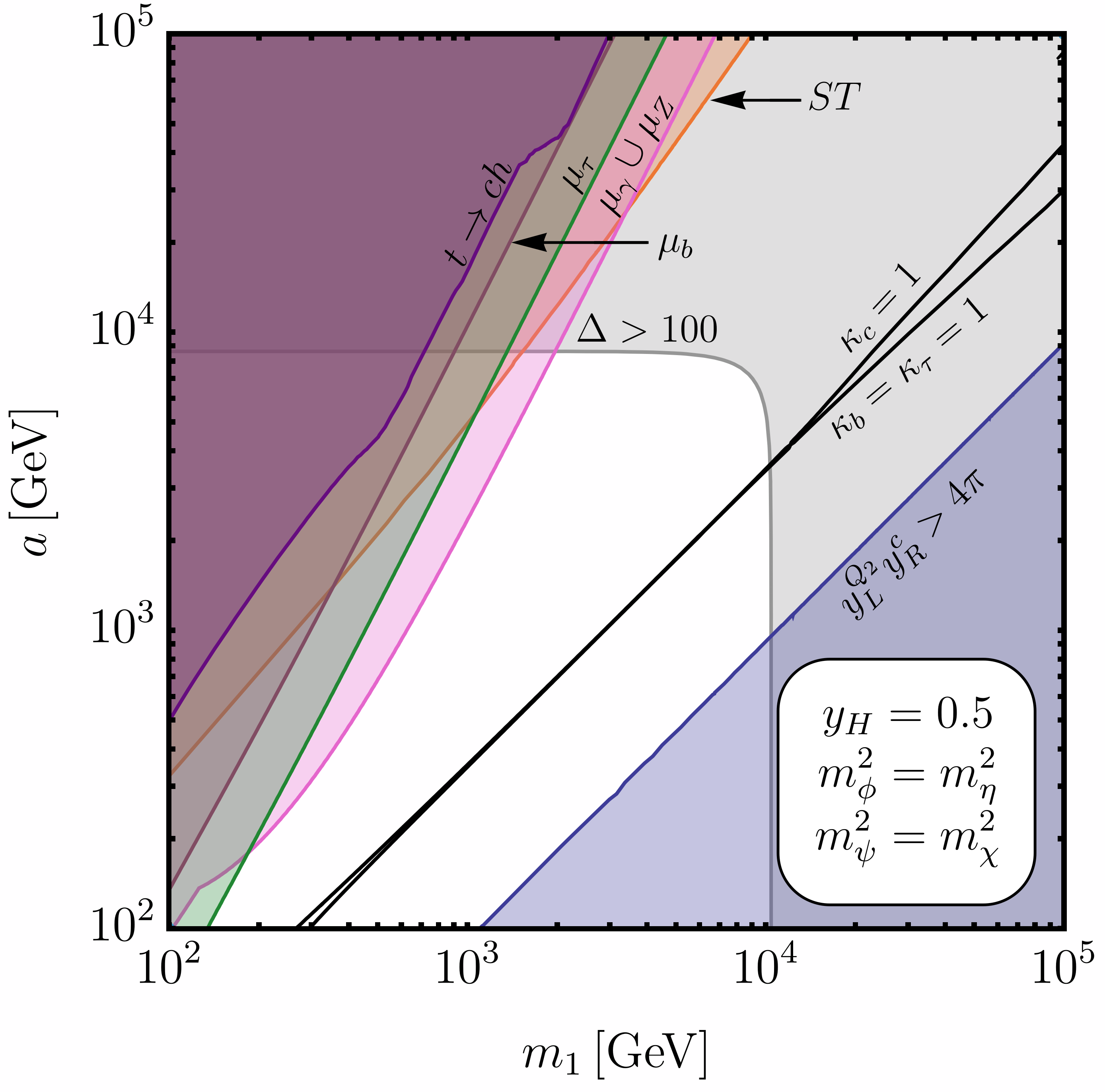
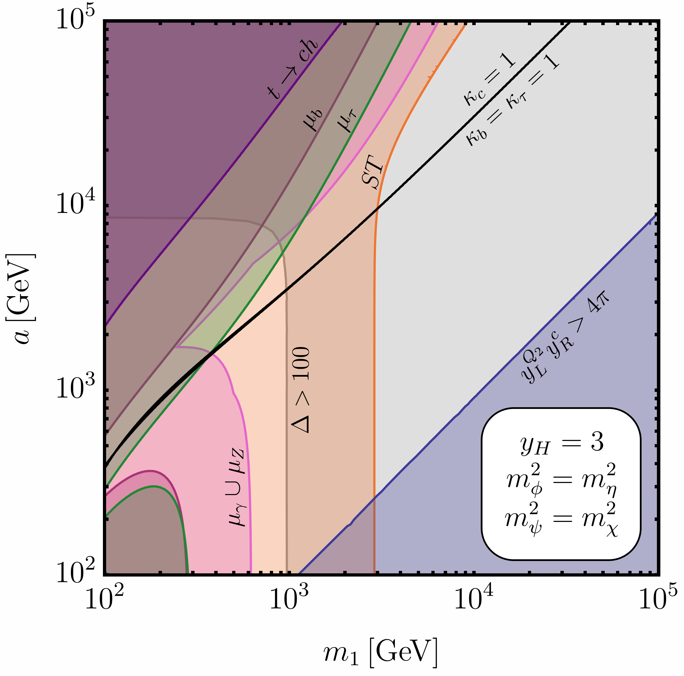

Exclusion plots using these constraints are shown for various slices of parameter space in Figure 5. The and bounds are combined for visual clarity, though is typically stronger. Constraints from projected future sensitivities are shown in Figure 6, assuming central values for each measurement at the SM prediction. Projected bounds are weaker than the current experimental constraints, and so are not shown.


The existence of unshaded regions demonstrates that viable parameter space currently exists for this model without excessive fine-tuning. Additionally, there are points within these regions with that are thus impossible to rule out by improving precision on while agreement with the SM is maintained. To exclude these points, one would need more precise bounds on and , or to carefully recast bounds from direct searches at colliders. Alternatively, such a model may be able to account for a small disparity between signal strength bounds and SM prediction, were one to arise in the future. Previous models in the framework could account for signal strengths slightly above unity, whereas hybrid models could account for measurements slightly below unity as well.
Of the experimental constraints, the parameters and typically provide the most stringent bounds for this model, including in future projections. There are multiple reasons for this. First, minimal hybrid models see larger corrections to these than previously considered models, as there is both a colour factor enhancement and contributions from both exotic fermion and scalar sectors. Second, the hybrid form of the Yukawa couplings can bring them into closer alignment with SM predictions, thus weakening the corresponding fermion signal strength bounds. Finally, the current 2 lower bound on is 0.98, thus small decreases in or increases in can quickly bring the predicted into conflict with experiment.
Since the exotics are charged under , we expect direct searches at colliders to provide significant constraints. As we have taken to be either unbroken or only broken by terms with small couplings, the lightest exotic field should be collider stable. The relevant searches are for -hadrons, as long-lived coloured exotics will hadronise with coloured SM fields to form at least quasi-stable particles. If is the lightest exotic, the existing bound on long lived sbottoms would enforce GeV Aaboud and others (2019b). We would expect a similar bound on from recast searches if it was instead the lightest exotic. These bounds exclude a significant portion of the available parameter space not ruled out by other constraints or subject to a high degree of fine-tuning. Future experiments could see up to a 10x improvement to this bound de Blas and others (2025), which could drastically reduce the viable parameter space without a fine-tuning problem, or remove it altogether. Since all hybrid models in the catalogue contain only coloured exotics, we would expect similar limitations on their parameter spaces.
4 Conclusion
We have detailed an extension to an earlier framework for generating one-loop SM fermion masses and Yukawa couplings. We then classified all minimal models capable of generating one-loop masses for the bottom, charm, and tau within this framework, to explain why their masses are near the GeV level. We found there exist 25 such models, eight of which are “hybrid” models; these have multiple topologies for the effective Yukawa coupling diagrams, and had not been previously studied in this framework. We analysed one of these hybrid models as a benchmark, and found that there currently exists parameter space where it is not ruled out or subject to a high degree of fine-tuning. We also showed that due to its hybrid nature, it was capable of producing effective Yukawa couplings greater than, less than, and exactly equal to the corresponding SM Yukawa couplings, demonstrating that the SM tree level mass-Yukawa coupling relationship can be produced by radiative mass models. If future measurements are found to be in tension with the SM relationship, such models may also be capable of explaining a discrepancy in either direction. It must be emphasised that even if agreement is maintained, these models will not necessarily be ruled out, but will be restricted to regions of parameter space with greater amounts of fine-tuning. Other individual models in the catalogue also have unique features that may be worth exploring, such as the viability of dark matter candidates, mass-mixing between three or more exotic fields, and/or the potential for an axion to be introduced. Most importantly, future work is needed to construct a complete model generating all SM fermion masses at the appropriate orders, using the catalogue here as a basis for further model-building. Flavour phenomenology for the lighter SM fermions is more tightly constrained, and may provide the strongest bounds on a complete model, though we expect that these would predominantly restrict the new parameters introduced to construct such a theory.
Acknowledgements.
We thank Peter Cox for helpful discussions. This work was supported in part by the Australian Research Council through the ARC Discovery Project grant DP260104148. LS is supported by an Australian Government Research Training Program Scholarship and the Rowden White Scholarship.Appendix A Three-exotic models
Let be distinct chiral fermions with right-handed components that do not transform under . Consider trying to generate all three of their masses at one-loop level within this framework, while introducing only three exotic fields. Without loss of generality, we can let these three fields be .
Now we note that and have the same spin, which is different from that of . Since this is also a property we require of and , it must be that and are either the same as or the conjugate of . Thus
| (25) |
Similarly, and transform the same way under , and differently to how transforms. By analogous argument it is clear that and are the same as or the conjugate of . Finally, this means that and must be identified with or its conjugate. Therefore
| (26) |
The term that couples to and requires that , and similarly for and . From the above logic, we have that
| (27) |
likewise must be in this set.
So
| (28) |
We therefore conclude that since , it is impossible to produce a three-exotic model in our framework for .
References
- Cross-section measurements of the Higgs boson decaying into a pair of -leptons in proton-proton collisions at TeV with the ATLAS detector. Phys. Rev. D 99, pp. 072001. External Links: 1811.08856, Document Cited by: Table 4, Table 4.
- Search for heavy charged long-lived particles in the ATLAS detector in 36.1 fb-1 of proton-proton collision data at TeV. Phys. Rev. D 99 (9), pp. 092007. External Links: 1902.01636, Document Cited by: §3.3.
- Higgs boson production cross-section measurements and their EFT interpretation in the decay channel at 13 TeV with the ATLAS detector. Eur. Phys. J. C 80 (10), pp. 957. Note: [Erratum: Eur.Phys.J.C 81, 29 (2021), Erratum: Eur.Phys.J.C 81, 398 (2021)] External Links: 2004.03447, Document Cited by: Table 4, Table 4.
- Measurements of and production in the decay channel in collisions at 13 TeV with the ATLAS detector. Eur. Phys. J. C 81 (2), pp. 178. External Links: 2007.02873, Document Cited by: Table 4, Table 4.
- Measurement of the properties of Higgs boson production at TeV in the channel using fb-1 of collision data with the ATLAS experiment. JHEP 07, pp. 088. External Links: 2207.00348, Document Cited by: Table 4, Table 4.
- Handbook of LHC Higgs Cross Sections: 3. Higgs Properties. . External Links: 1307.1347, Document Cited by: §3.3.
- Sequentially loop suppressed fermion masses from a single discrete symmetry. JHEP 06, pp. 043. External Links: 1911.02033, Document Cited by: §1.
- Radiative Mechanisms for Generating Quark and Lepton Masses: Some Recent Developments. Mod. Phys. Lett. A 4, pp. 1975. External Links: Document Cited by: §1.
- Has the Origin of the Third-Family Fermion Masses been Determined?. JHEP 04, pp. 151. External Links: 2012.10458, Document Cited by: §1, §2.2, §2, §3.2, §3.3.
- Radiative muon mass models and . JHEP 05, pp. 174. External Links: 2103.13401, Document Cited by: §1.
- Quark Mixings and Mass Hierarchy From Radiative Corrections. Phys. Lett. B 205, pp. 345–352. External Links: Document Cited by: §1.
- Fermion mass hierarchy in an extended left-right symmetric model. JHEP 12, pp. 075. External Links: 2305.11967, Document Cited by: §1.
- Radiatively generated hierarchy of lepton and quark masses. JHEP 02, pp. 125. External Links: 1611.09797, Document Cited by: §1.
- Maximal Abelian Flavor Symmetries. External Links: 2606.07799 Cited by: footnote 2.
- Naturalness made easy: two-loop naturalness bounds on minimal SM extensions. JHEP 02, pp. 129. External Links: 1607.07446, Document Cited by: §3.3.
- LHC HXSWG interim recommendations to explore the coupling structure of a Higgs-like particle. . External Links: 1209.0040 Cited by: §3.3.
- Quark mass hierarchies from universal seesaw mechanism. Phys. Rev. D 49, pp. 1378–1388. External Links: Document Cited by: footnote 2.
- Quark Masses and Mixing Angles From Universal Seesaw Mechanism. Phys. Rev. D 41, pp. 208. External Links: Document Cited by: footnote 2.
- Linking geometric mass hierarchy with threefold family replication. J. Phys. G 25, pp. 1571–1588. External Links: hep-ph/9802235, Document Cited by: footnote 2.
- Universal Seesaw Mechanism?. Phys. Rev. Lett. 59, pp. 393. External Links: Document Cited by: footnote 2.
- Family Mass Hierarchy From Universal Seesaw Mechanism. Phys. Rev. Lett. 60, pp. 1813. External Links: Document Cited by: footnote 2.
- Higgs Boson Studies at Future Particle Colliders. JHEP 01, pp. 139. External Links: 1905.03764, Document Cited by: Figure 6, Figure 6.
- Electroweak precision observables and Higgs-boson signal strengths in the Standard Model and beyond: present and future. JHEP 12, pp. 135. External Links: 1608.01509, Document Cited by: Figure 6, Figure 6.
- Physics Briefing Book: Input for the 2026 update of the European Strategy for Particle Physics. External Links: 2511.03883, Document Cited by: §3.3.
- Quark and lepton masses from top loops. JHEP 08, pp. 100. External Links: 0805.0822, Document Cited by: §1.
- Physics briefing book: input for the european strategy for particle physics update 2020. . External Links: 1910.11775 Cited by: §3.3.
- Anomalous Higgs Yukawa Couplings. EPL 108 (1), pp. 11002. External Links: 1402.6415, Document Cited by: §1.
- Hierarchy of Quark Masses, Cabibbo Angles and CP Violation. Nucl. Phys. B 147, pp. 277–298. External Links: Document Cited by: footnote 2.
- A Geometry of the generations. Phys. Rev. Lett. 75, pp. 3985–3988. External Links: hep-ph/9508296, Document Cited by: footnote 2.
- Radiative Generation of Quark and Lepton Mass Hierarchies From a Top Quark Mass Seed. Phys. Rev. D 41, pp. 1630. External Links: Document Cited by: §1.
- Radiative origin of fermion mass hierarchy in left-right symmetric theory. JHEP 01, pp. 082. External Links: 2409.04246, Document Cited by: §1.
- Fermion masses and mixing angles from SU(3) family symmetry. Phys. Lett. B 520, pp. 243–253. External Links: hep-ph/0108112, Document Cited by: footnote 2.
- Hierarchical Radiative Quark and Lepton Mass Matrices. Phys. Rev. Lett. 64, pp. 2866–2869. External Links: Document Cited by: §1.
- Radiative Origin of All Quark and Lepton Masses through Dark Matter with Flavor Symmetry. Phys. Rev. Lett. 112, pp. 091801. External Links: 1311.3213, Document Cited by: §1.
- Radiatively generated fermion mass hierarchy from flavor nonuniversal gauge symmetries. Phys. Rev. D 106 (7), pp. 075020. External Links: 2207.10407, Document Cited by: §1.
- Partially flavour non-universal U(1) and radiative fermion masses. JHEP 02, pp. 170. External Links: 2508.05439, Document Cited by: §1.
- A New constraint on a strongly interacting Higgs sector. Phys. Rev. Lett. 65, pp. 964–967. External Links: Document Cited by: §3.3.
- Estimation of oblique electroweak corrections. Phys. Rev. D 46, pp. 381–409. External Links: Document Cited by: §3.3.
- Horizontal symmetries for the supersymmetric flavor problem. Nucl. Phys. B 466, pp. 3–24. External Links: hep-ph/9507462, Document Cited by: footnote 2.
- Seesaw Masses for Quarks and Leptons in an Ambidextrous Electroweak Interaction Model. Phys. Lett. B 191, pp. 122–126. External Links: Document Cited by: footnote 2.
- Higgs Yukawa coupling constraints on a benchmark one-loop radiative mass model for the bottom, charm and tau. External Links: 2511.08924 Cited by: §1, §1, §2.3, §2, §3.
- Review of Particle Physics. Int. J. Mod. Phys. A 41, pp. 2630011. External Links: Document Cited by: §3.3, Table 4, Table 4.
- A portrait of the Higgs boson by the CMS experiment ten years after the discovery.. Nature 607 (7917), pp. 60–68. Note: [Erratum: Nature 623, (2023)] External Links: 2207.00043, Document Cited by: Table 4, Table 4.
- Search for Higgs Boson Decay to a Charm Quark-Antiquark Pair in Proton-Proton Collisions at s=13 TeV. Phys. Rev. Lett. 131 (6), pp. 061801. External Links: 2205.05550, Document Cited by: Table 4, Table 4.
- Electromagnetic and weak masses. Phys. Rev. Lett. 29, pp. 388–392. External Links: Document Cited by: §1.
- Models of Lepton and Quark Masses. Phys. Rev. D 101 (3), pp. 035020. External Links: 2001.06582, Document Cited by: §1.