SciFigPlag-Bench: A Benchmark for Provenance-Aware Scientific Figure Plagiarism Detection

Zhiying Cui Minghao Yang Linlin Gao Jie Liu Pengyuan Li

Abstract

Scientific figures often encode the visual evidence behind scientific findings, yet figure plagiarism remains underexplored as a benchmarked multimodal evaluation problem. We present SciFigPlag-Bench, a benchmark for provenance-aware reasoning over scientific figures in scholarly documents. Unlike general image-similarity or image-forensics benchmarks, SciFigPlag-Bench evaluates whether a suspicious reuses evidence from a specific source figure, how the reused content has been transformed, and where the reused evidence appears. We introduce a factorized taxonomy that separates what is reused from how it is transformed, covering material-preserving reuse, such as full-figure and subfigure reuse, as well as abstract-content reuse, such as data re-expression and structural redraw. Guided by this taxonomy, we construct a hybrid benchmark with 2,582 positive pairs and 2,541 negative pairs, combining documented real-world cases, taxonomy-guided synthetic examples, and visually similar negatives. The benchmark supports four diagnostic tasks: pairwise detection, source attribution, hierarchical reuse-type classification, and reuse correspondence localization. Experiments with diverse vision-language models establish initial baselines and reveal persistent challenges in fine-grained provenance reasoning, reuse-type understanding, and spatial evidence grounding.

Introduction

Refer to caption — Figure 1: Overview of SciFigPlag-Bench. The benchmark combines verified real-world plagiarism pairs, taxonomy-guided synthetic positive pairs, and visually similar negative pairs. It supports four evaluation tasks that progress from Pairwise Detection and Source Attribution to Reuse-Type Classification and Reuse Localization. VLMs are evaluated using standardized task-specific prompts, with their outputs assessed by the corresponding metrics.

Scientific figures are a central part of scholarly communication, carrying dense visual evidence such as experimental results, quantitative trends, methodological diagrams, and analytical interpretations. When figures are copied, relabeled, recombined, or redrawn without proper attribution, the provenance of scientific evidence becomes obscured, creating a serious research-integrity risk (4; 5; 42; 6). Although text plagiarism has mature screening workflows (14; 2; 32) and established benchmarks (9; 45; 44; 22; 19), scientific figure plagiarism has not been systematically formulated as an evaluation problem.

Benchmarking for image manipulation detection and localization has advanced rapidly, but most existing datasets are designed for natural-image authenticity analysis rather than scientific figure provenance. Standard forensic datasets—such as CASIA, Columbia, COVERAGE, NIST16, and IMD2020—are widely used for evaluating manipulation detection and mask localization (10; 29; 41; 27; 30). More recent datasets, including GIM (7) and COCO-Inpaint (43), extend evaluation to large-scale generative and inpainting scenarios. These benchmarks are valuable for determining whether an image has been manipulated and where manipulated pixels occur. However, they do not directly evaluate the central provenance question in scientific figure plagiarism: whether a suspicious figure reuses evidence from a specific source figure. Scientific figure reuse may involve copied panels, localized regions, recomposed multi-panel layouts, quantitative data re-expression, or structural redraw, rather than only pixel-level manipulation.

A smaller but more directly relevant line of work has studied plagiarism detection for non-textual and multimodal document content (24; 23; 11; 12; 5). Early studies compared images extracted from documents using feature-point matching or content-based image retrieval, noting that document plagiarism systems often overlook non-textual material, even though reused figures can be highly informative for detecting concealed plagiarism. Subsequent work introduced adaptive image-based plagiarism detection pipelines for academic documents and hybrid systems such as HyPlag (24), which combine images with text, citations, and mathematical expressions to improve retrieval of suspicious source documents. Other figure-specific studies address narrower scientific subproblems, including bar-chart plagiarism, flowchart/diagram plagiarism, or semantic figure matching (23). However, these methods are typically evaluated in narrow settings, such as document-level retrieval, limited figure categories, or exact and near-exact reuse scenarios. It therefore remains unclear whether modern vision-language models can support the full provenance reasoning process required for scientific figure reuse: detecting reuse, attributing it to a source, characterizing the reuse-type, and localizing the reused evidence.

In this work, we introduce SciFigPlag-Bench¹¹ 1 Code and benchmark data will be publicly released upon acceptance; the code is included in the supplementary package., a benchmark for provenance-aware scientific figure plagiarism detection and analysis in scholarly documents. SciFigPlag-Bench evaluates whether a suspicious scientific figure reuses content from a specific source figure, and whether models can reason about the provenance relationship beyond generic image similarity. To support this goal, we propose a factorized taxonomy of scientific figure reuse that separates what is reused from how it is transformed. The taxonomy covers both material-preserving reuse, such as full-figure and subfigure reuse, and abstract-content reuse, such as data reuse and structural reuse. In particular, data-level and structural reuse capture challenging cases where a suspicious figure may re-express the same underlying data or redraw the same conceptual structure while sharing little direct visual overlap with the source.

Guided by this taxonomy, we construct a hybrid benchmark combining documented real-world plagiarism cases, taxonomy-guided synthetic examples, and visually similar negative data. This design combines realistic misconduct cases with controlled coverage of important reuse types, while testing whether models can distinguish true provenance reuse from superficial visual similarity. SciFigPlag-Bench supports four tasks: pairwise plagiarism detection, source attribution, hierarchical reuse-type classification, and reuse correspondence localization. These tasks evaluate not only whether reuse exists, but also which source was reused, how the reused content was transformed, and where the reused evidence appears. Finally, we benchmark a broad set of open- and closed-source vision-language models, establishing initial baselines and analyzing current capabilities and failure patterns in scientific figure plagiarism analysis.

SciFigPlag Taxonomy

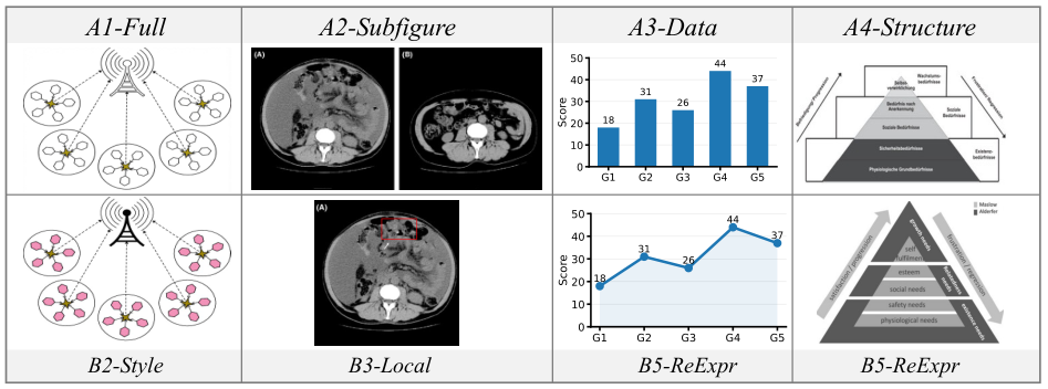
Scientific figure plagiarism extends beyond direct visual duplication. A suspicious figure may reuse a full figure, copy a panel or region, re-express the same quantitative data, or redraw the same conceptual structure. We capture this diversity with a dual-layer taxonomy: Layer A defines what is reused, and Layer B defines how it is modified. Appendix E provides detailed definitions and representative examples for all Layer A reuse types and Layer B modification types.

Layer A: Reused content type.

Layer A describes what is reused from the source figure and defines four mutually exclusive primary reuse types. Material-preserving reuse covers cases that retain source visual material: A1-Full reuses an entire figure, while A2-Subfigure reuses a panel, region, or visual component. Abstract-content reuse covers cases that do not preserve the original visual artifact: A3-Data reuses the same quantitative data, and A4-Structure reuses the same structural, procedural, or topological logic.

Layer B: Modification type.

Layer B describes how reused content is modified. It includes direct preservation (B1-Direct), style modification (B2-Style), local editing (B3-Local), geometric transformation (B4-Geometry), and re-expression in a new visual form (B5-ReExpr).

Layer A–B compatibility.

Layer A and Layer B are not fully independent; valid combinations depend on whether the reuse preserves source visual material. As shown in Table 1, material-preserving reuse types (A1-Full, A2-Subfigure) pair with visual modifications B1–B4. Abstract-content reuse types (A3-Data, A4-Structure) are paired with B5-ReExpr, because they re-express data or structure rather than preserve pixels. This compatibility design allows each positive pair to be annotated by both what is reused and how it is modified, while keeping Layer A categories mutually exclusive.

Reuse type	B1	B2	B3	B4	B5
A1	$\checkmark$	$\checkmark$	$\checkmark$	$\checkmark$	–
A2	$\checkmark$	$\checkmark$	$\checkmark$	$\checkmark$	–
A3	–	–	–	–	$\checkmark$
A4	–	–	–	–	$\checkmark$

Table 1: Valid Layer-A–B label combinations in the SciFigPlag taxonomy.

SciFigPlag-Bench Dataset Construction

SciFigPlag-Bench comprises three complementary data components: documented real-world plagiarism cases, taxonomy-guided synthetic reuse examples, and visually similar negative data.

Overall, the benchmark contains 15,348 images, covering authentic plagiarism patterns, controlled coverage of underrepresented reuse types, and challenging non-plagiarized pairs. Figure 3 summarizes the overall data composition and pair distribution. Figures 3(a) and 3(b) further show the Layer-A reused content type and Layer-B modification type distributions over all positive pairs.

Real-world Figure Plagiarism Cases

Real-world figure plagiarism cases are difficult to collect at scale because they require documented source–suspicious correspondences and careful manual verification. We therefore curate real-world positives from two publicly available resources that provide rare examples of scientific figure reuse. The first source is VroniPlag Wiki (8), a community-maintained resource documenting plagiarism cases in academic work, including cases where figures or figure components are reused from identifiable sources. The second source is the Mendeley Figure Plagiarism Detection corpus (13), a public dataset constructed for figure plagiarism detection.

Because these resources contain heterogeneous cases and may include examples that are unsuitable for our benchmark, we manually verify all candidate pairs. From VroniPlag Wiki (39), we extract 553 manipulated–source pairs and remove 13 pairs that do not represent valid figure-plagiarism cases after inspection. From the Mendeley corpus (13), we retain 104 valid pairs after verifying that each pair contains a usable figure-level correspondence. This filtering step removes noisy or ambiguous cases and ensures that the retained examples provide reliable source–suspicious relationships.

Data Annotation

After this manual screening and verification, the 644 retained real-world pairs were annotated according to the SciFigPlag taxonomy. Three annotators independently examined each source–suspicious pair and assigned one mutually exclusive Layer-A label and all applicable Layer-B labels subject to the A–B compatibility constraints in Table 1. Multiple Layer-B labels were assigned when several modification types co-occurred in a real-world pair. The independent annotations were then compared, and disagreements were jointly reviewed and resolved by consensus. The consensus labels serve as the ground truth for these real-world positive pairs shown in Figure 3(c).

Taxonomy-Guided Synthetic Reuse Data

Real-world cases provide high-fidelity examples but are limited in scale and coverage, especially for less common reuse types. As shown in Figure 3(c), we therefore generate taxonomy-guided synthetic examples to expand Layer-A/B coverage while complementing the real-world subset. We do not synthesize A4-Structure cases because high-level structural reuse is difficult to generate with reliable quality. Instead, all A4-Structure examples are taken from real-world cases. The generation process follows the Layer A–B compatibility structure summarized in Table 1. Each synthetic pair is generated with a single controlled Layer-B modification and therefore has a single Layer-B ground-truth label. Figure 2 illustrates representative examples under this taxonomy-guided design.

(a) Layer-A distribution

(b) Layer-B distribution

(d) Overall pair composition

Figure 3: Data composition of SciFigPlag-Bench. (a) Layer-A distribution over positive pairs. (b) Layer-B label distribution; some real-world pairs have multiple Layer-B labels. (c) Positive-pair composition by data source and Layer-A/B type. (d) Overall composition of real-world positives, synthetic positives, and visually similar negatives.

Full-Figure Reuse.

Synthetic A1-Full pairs are constructed from figures in the PubMed Open Access Subset (28). Each pair is constructed using one of the four Layer-B modification types (B1–B4), as summarized in Appendix Table 7. Specifically, B1-Direct, B3-Local, and B4-Geometry modifications are applied programmatically, whereas B2-Style modifications are generated using Gemini 3 Pro Image (15) with the prompt in Appendix D.

Subfigure Reuse.

Synthetic A2-Subfigure pairs are generated from compound figures collected from PubMed (28) to capture localized content reuse. Candidate subfigures are segmented using a VLM (Qwen3.5B-Flash (35)) with the prompt provided in Appendix D, and then manually curated to ensure accurate ground-truth annotations. Each subfigure is then transformed using the same B operations (Table 7) as A1-Full pairs, producing controlled variations with localized modifications while preserving content.

In addition, we construct composite figures by combining a synthetic reused subfigure with one or three negative distractors, forming 2-panel and 4-panel layouts while retaining the ground-truth location of the reused subfigure. These composites introduce diverse layouts and subtle visual variations, creating challenging examples that require models to identify the reused content within visually similar surrounding panels.

Data Reuse.

For A3-Data, we use the ChartNet dataset (21), which provides CSV data along with 24 chart types, enabling both preservation of underlying semantics and diverse visual representations. From this dataset, 579 chart instances were selected and programmatically redrawn from their CSV files to generate synthetic positive pairs. Seven chart types were produced for reuse, including line, bar, area, radar, bubble, heatmap, and 3D heatmap charts. This process ensures that the original data remains unchanged while expanding the visual diversity for synthetic data reuse.

Negative Data Collection

Negatives provide challenging non-plagiarized examples that are visually or semantically similar to source figures. For each real-world and synthetic source figure, we retrieve visually similar images using the Google Lens visual-search API provided by SearchApi (37). We collect the top $K=8$ matches and discard the first result to reduce the chance of retaining the original image or an exact duplicate. We then manually inspect the remaining candidates to remove ambiguous cases and images that may reuse content from the source figure. After filtering and deduplication, we obtain 10,184 negative images.

The negative data pool is used in three ways: 2,541 negatives are paired with source figures to form visually or semantically similar non-plagiarized pairs; 2,904 negatives are used as distractor panels in composite-figure construction; and the pool is also used to provide visually similar distractors for constructing candidate sets that do not contain the ground-truth source.

Benchmark Tasks.

Scientific figure plagiarism analysis involves multiple stages, including detecting plagiarism, identifying the source figure, classifying the reuse type, and localizing the corresponding regions. Accordingly, we design four tasks to systematically assess VLM capabilities across these stages.

Pairwise Detection.

This task evaluates whether plagiarism exists between a pair of figures. Given a source figure $I_{s}$ and a suspicious figure $I_{q}$ , the model predicts a binary label $y\in\{\texttt{yes},\texttt{no}\}$ based on the reused content types defined in the SciFigPlag taxonomy. We report accuracy, precision, recall, and F1 score.

Source Attribution.

This task evaluates source attribution: given a suspicious figure $I_{q}$ and four candidate source figures $\{I_{A},I_{B},I_{C},I_{D}\}$ , the model identifies which candidate $I_{q}$ is reused from, or predicts N if none applies. We use accuracy as the evaluation metric.

Reuse-Type Classification.

This task evaluates how a source figure $I_{s}$ is reused in a suspicious figure $I_{q}$ . The model predicts exactly one Layer-A label for what content is reused and one or more Layer-B labels for how it is modified. We report Layer-A, Layer-B, and joint accuracy, where Layer-B accuracy uses strict exact-set matching, with partial matches counted as incorrect. Joint accuracy requires both the Layer-A label and the complete Layer-B label set to be correct.

Size	Model	PairDet				SrcAttr	ReuseType			ReuseLoc			Overall
Size	Model	Acc	Prec	Rec	F1	Acc	A-Acc	B-Acc	Joint	Src	Comp	Pair	Avg
Small	InternVL-3.5-2B-Flash^†	58.0	76.1	23.8	36.3	64.0	45.1	20.8	13.7	0.4	0.0	0.0	33.9
	Qwen-3.5-2B^†,⋆	75.3	69.6	90.6	78.8	29.4	48.7	30.1	17.9	7.4	4.6	0.8	30.9
	Granite-4-3B-Vision^†	65.7	64.1	66.7	65.4	24.1	40.6	19.5	10.8	14.9	7.2	1.3	25.5
	Gemma-3-4B	67.4	63.5	83.4	72.1	29.1	47.4	23.8	17.6	4.6	1.5	0.2	28.6
Medium	InternVL-3.5-8B^†	74.4	74.1	75.6	74.9	64.4	74.1	46.1	43.9	1.5	1.3	0.3	45.8
	Pixtral-12B^†	52.1	51.4	96.0	66.9	67.7	52.3	18.5	12.5	4.9	3.6	0.2	33.1
	Phi-4-15B-Vision^†,⋆	54.8	53.7	76.6	63.1	7.5	52.3	31.8	28.4	14.7	21.4	3.3	23.5
Large	Gemma-4-26B-A4B^⋄,⋆	87.2	81.0	97.6	88.5	62.2	85.4	64.5	58.8	19.8	15.9	5.8	53.5
	Gemma-4-31B^⋆	92.5	88.1	98.5	93.0	92.6	96.9	70.7	70.6	81.2	85.0	75.2	82.7
	Qwen-3.6-35B-A3B^⋄,⋆	87.0	80.0	99.1	88.5	97.6	92.9	69.4	68.4	81.1	79.2	69.0	80.5
	Qwen-3.5-35B-A3B^⋄,⋆	87.3	81.0	98.7	89.0	97.8	94.4	70.1	69.8	79.7	75.8	64.1	79.8
	InternVL-3.5-38B^†	86.5	83.0	92.0	87.2	81.3	81.5	56.4	50.5	21.1	15.2	7.9	56.6
	Mistral-Small-4-119B-A6B^⋄,⋆	81.0	77.1	88.8	82.5	24.9	74.6	45.4	41.9	10.3	5.1	1.2	37.3
Closed	Gemini-3-Flash^⋆	91.4	85.9	99.4	92.2	97.8	95.8	71.9	71.7	80.8	77.9	71.0	83.0
	Claude-Sonnet-4.6^⋆	96.3	93.3	99.8	96.4	98.1	87.3	54.5	51.7	73.8	84.4	64.2	77.6
	GPT-5.4^⋆	84.4	76.8	99.0	86.5	97.1	90.1	68.9	65.5	79.6	85.4	73.5	80.1

Table 2: Main results across four tasks. All values are percentages (%). Overall is the average of PairDet Acc, SrcAttr Acc, ReuseType Joint, and ReuseLoc Pair. Bold indicates the best result in each column.

Note. ^† Models evaluated with local inference. ^⋄ Mixture-of-Experts model. ^⋆ Reasoning/thinking model.

Reuse Localization.

This task evaluates localized spatial correspondence between reused regions and is therefore restricted to A2-Subfigure pairs with B1–B4 modifications. For each pair, the model predicts one bounding box in the source figure $I_{s}$ and one in the suspicious figure $I_{q}$ , each represented by its normalized top-left and bottom-right coordinates. We report localization accuracy at IoU $\geq$ 0.5 for the source-side box (Src), the suspicious composite-side box (Comp), and the paired prediction (Pair). Pair is correct only when both boxes meet the threshold.

Experiments

We evaluate VLMs on the four benchmark tasks: pairwise detection (PairDet), source attribution (SrcAttr), reuse-type classification (ReuseType), and reuse localization (ReuseLoc). Our experiments aim to establish reference baselines for provenance-aware scientific figure plagiarism analysis and to examine how model performance changes as the evaluation progresses from coarse reuse detection to source attribution, reuse-type reasoning, and spatial localization.

Experimental Settings

We evaluate a diverse set of VLMs across different capability levels, covering small, medium, large, and closed-source frontier models. Small models include InternVL-3.5-2B-Flash, Qwen-3.5-2B, Gemma-3-4B, and Granite-4-3B-Vision (40; 33; 16; 20). Medium models include InternVL-3.5-8B, Pixtral-12B, and Phi-4-15B-Vision (40; 1; 25). Large models include InternVL-3.5-38B, Qwen-3.6-35B-A3B, Qwen-3.5-35B-A3B, Gemma-4-26B-A4B, Gemma-4-31B, and Mistral-Small-4-119B-A6B (40; 36; 34; 17; 26). Closed-source models include representative frontier VLMs, namely Claude-Sonnet-4.6, GPT-5.4, and Gemini-3-Flash (3; 31; 18).

Overall, the model suite covers open-weight VLMs with a wide range of parameter scales, including both dense and mixture-of-experts (MoE) architectures (38), together with closed-source frontier VLMs for comparison. All models are evaluated using the same task-specific prompts with temperature set to zero. The prompts and detailed model information are provided in Appendix D and Table 8.

Main Results

Overall performance.

Table 2 reports the main results across the four benchmark tasks. Detailed task-wise breakdowns are provided in Appendix G. Overall performance is highly polarized rather than smoothly distributed. Only a few models achieve strong average scores, including Gemini-3-Flash with the best overall score of 83.0, followed by Gemma-4-31B with 82.7, Qwen-3.6-35B-A3B with 80.5, GPT-5.4 with 80.1, and Qwen-3.5-35B-A3B with 79.8. This indicates that the strongest recent open-weight VLMs are competitive with closed-source frontier models at the aggregate level.

However, high overall scores mask task-specific weaknesses. For example, Gemini-3-Flash achieves the best overall score but obtains only 71.0 on ReuseLoc Pair, while GPT-5.4 reaches 80.1 overall but only 65.5 on ReuseType Joint. Meanwhile, most small and medium models remain far behind, with medium-model overall scores ranging from 23.5 to 45.8. These results indicate scientific figure plagiarism understanding remains challenging, especially for fine-grained reuse-type reasoning and correspondence localization.

Model scaling.

Model scale is an important but incomplete predictor of performance. As shown in Table 2 and Figure 5, large models generally outperform small and medium models. The trend is especially clear within the InternVL-3.5 family, where the overall score increases from 33.9 for InternVL-3.5-2B-Flash, to 45.8 for InternVL-3.5-8B, and further to 56.6 for InternVL-3.5-38B. This monotonic within-family improvement suggests that scaling benefits provenance-aware scientific figure understanding. Nevertheless, InternVL-3.5-38B still trails the leading models by over 20 points, indicating that scale alone cannot account for strong performance.

MoE architectures.

Some MoE models achieve favorable parameter–performance trade-offs when evaluated by active parameters. For example, Qwen-3.6-35B-A3B and Qwen-3.5-35B-A3B achieve strong overall scores of 80.5 and 79.8 while activating only a small subset of their total parameters. However, MoE design does not guarantee strong performance: Gemma-4-26B-A4B and Mistral-Small-4-119B-A6B obtain much lower overall scores of 53.5 and 37.3. These results suggest that sparse activation alone is insufficient; strong performance also depends on broader visual reasoning and grounding capabilities.

Task-wise Analysis

Pairwise detection.

PairDet is the most accessible task, yet remains clearly scale-sensitive. Large and closed-source models perform substantially better than small and medium models: Claude-Sonnet-4.6, Gemini-3-Flash, and Gemma-4-31B all exceed 90% accuracy, while several smaller models remain below 60%. Figure 4 shows that weaker models fail across multiple reuse categories rather than on a single subtype. A3-Data and B5-ReExpr are relatively easier in PairDet, suggesting that direct pairwise comparison helps models recognize coarse data or structural reuse.

Figure 6: Subset-wise performance across model tiers. We compare real-world and synthetic subsets for PairDet, SrcAttr, and ReuseType using task-specific core metrics. Solid bars indicate real-world samples and hatched bars indicate synthetic samples, with vertical dashed lines separating small, medium, large, and closed-source models.

Source attribution.

SrcAttr is more discriminative because the model must identify the true source among multiple plausible candidates. Performance is highly separated: strong models such as Claude-Sonnet-4.6, Gemini-3-Flash, and Qwen-3.5-35B-A3B reach around 98% accuracy, whereas Mistral-Small-4-119B-A6B drops to 24.9%. However, attribution is not determined by scale alone, as InternVL-3.5-2B-Flash achieves 64.0%, outperforming several larger models. Compared with PairDet, A3-Data and B5-ReExpr become more fragile for many models, indicating that recognizing reuse is easier than attributing it to the correct source under similar distractors.

Reuse-type classification.

ReuseType tests whether models can characterize the plagiarism pattern beyond detection. The main bottleneck is Layer-B modification classification: Gemini-3-Flash drops from 95.8% on Layer-A to 71.9% on Layer-B, GPT-5.4 from 90.1% to 68.9%, and Gemma-4-31B from 96.9% to 70.7%. This gap shows that current VLMs are better at identifying what content is reused than determining how it has been transformed. Fine-grained reuse characterization therefore remains a major challenge.

Reuse localization.

ReuseLoc is the most demanding task because it requires coordinate-level correspondence grounding in both images. Only a few models, including Gemma-4-31B, GPT-5.4, Gemini-3-Flash, Qwen-3.6-35B-A3B, Claude-Sonnet-4.6, and Qwen-3.5-35B-A3B, achieve appreciable Pair scores, while most models score near zero; even the best score is below 76%. Output-validity and qualitative analyses show that these low scores mainly reflect spatial-grounding errors rather than malformed outputs, revealing a key limitation of current VLMs in correspondence localization (Appendix Table 5 and Figure 9).

Data-Source Analysis

Real-world vs. synthetic subsets.

Figure 6 compares real-world and synthetic subsets for PairDet, SrcAttr, and ReuseType. For PairDet and SrcAttr, strong models achieve similar performance on the two subsets, suggesting that synthetic examples do not form trivially separable cases.

In contrast, ReuseType shows a clearer real–synthetic gap in Layer-B and joint accuracy, both requiring exact Layer-B label-set matching. Unlike synthetic pairs with one controlled Layer-B label, real-world pairs may contain multiple co-occurring labels. To examine this effect, we report relaxed joint accuracy, requiring the correct Layer-A label and at least one matched Layer-B label. Under this criterion, the real–synthetic gap largely disappears, indicating that the gap under strict evaluation mainly reflects the exact-set requirement for multi-label real-world pairs (Appendix Table 4).

Negatives in PairDet.

Figure 7 further decomposes PairDet accuracy into real-world positives, synthetic positives, and visually similar negatives. While strong models are relatively balanced on real-world and synthetic positives, the negative subset exposes clearer failure modes. Several small and medium models show strong label biases: for example, Pixtral-12B most severely over-predicts plagiarism for visually similar negatives, while InternVL-3.5-2B-Flash shows the opposite bias, under-predicting plagiarism and missing many positive pairs. These results confirm the importance of visually similar negatives in PairDet evaluation. Without them, models could achieve inflated scores by exploiting superficial similarity or label priors rather than identifying true provenance reuse. Even for stronger models, negative accuracy remains lower in several cases, indicating that separating genuine reuse from strong visual similarity is still non-trivial.

Together, these results show that synthetic examples provide a useful controlled complement to real-world cases, while negatives are essential for testing whether models capture true provenance reuse rather than superficial visual similarity.

Figure 7: Pairwise detection accuracy on real-world positive pairs, synthetic positive pairs, and negative pairs.

Conclusion

We present SciFigPlag-Bench, a benchmark for provenance-aware reasoning over scientific figures in scholarly documents. Built on a two-layer taxonomy separating reused content from modification types, it evaluates pairwise detection, source attribution, reuse-type classification, and reuse localization using real-world cases, taxonomy-guided synthetic samples, and visually similar negatives. Together, these tasks span reuse detection, characterization, and localization. Experiments show that even strong vision-language models struggle with fine-grained reuse-type reasoning and spatial grounding, motivating more reliable, evidence-grounded methods for multimodal scientific document analysis.

References

Agrawal et al. (2024) P. Agrawal et al. Pixtral 12B. arXiv preprint arXiv:2410.07073. External Links: Link Cited by: Experimental Settings.
Amirzhanov et al. (2025) A. Amirzhanov, C. Turan, and A. Makhmutova Plagiarism types and detection methods: a systematic survey of algorithms in text analysis. Frontiers in Computer Science 7, pp. 1504725. External Links: Document, Link Cited by: Introduction.
Anthropic (2026) Anthropic Introducing Claude Sonnet 4.6. Note: Blog postAccessed: 2026-05-25 External Links: Link Cited by: Experimental Settings.
Bik et al. (2016) E. M. Bik, A. Casadevall, and F. C. Fang The prevalence of inappropriate image duplication in biomedical research publications. mBio 7 (3), pp. e00809–16. External Links: Document Cited by: Introduction.
Bucci (2018) E. M. Bucci Automatic detection of image manipulations in the biomedical literature. Cell Death & Disease 9 (3), pp. 400. External Links: Document Cited by: Introduction, Introduction.
Candal-Pedreira et al. (2022) C. Candal-Pedreira, J. S. Ross, A. Ruano-Ravina, D. S. Egilman, E. Fernández, and M. Pérez-Ríos Retracted papers originating from paper mills: cross sectional study. BMJ 379, pp. e071517. External Links: Document Cited by: Introduction.
Chen et al. (2025) Y. Chen, X. Huang, Q. Zhang, W. Li, M. Zhu, Q. Yan, S. Li, H. Chen, H. Hu, J. Yang, W. Liu, and J. Hu GIM: a million-scale benchmark for generative image manipulation detection and localization. In Proceedings of the AAAI Conference on Artificial Intelligence, Vol. 39, pp. 2311–2319. External Links: Document, Link Cited by: Introduction.
Dannemann (2018) G. Dannemann Crowd-based documentation of plagiarism: the VroniPlag wiki experience. In Research Ethics in the Digital Age: Ethics for the Social Sciences and Humanities in Times of Mediatization and Digitization, pp. 45–67. External Links: Document Cited by: Real-world Figure Plagiarism Cases.
Dolan and Brockett (2005) W. B. Dolan and C. Brockett Automatically constructing a corpus of sentential paraphrases. In Proceedings of the Third International Workshop on Paraphrasing (IWP2005), External Links: Link Cited by: Introduction.
Dong et al. (2013) J. Dong, W. Wang, and T. Tan CASIA image tampering detection evaluation database. In 2013 IEEE China Summit and International Conference on Signal and Information Processing, pp. 422–426. External Links: Document Cited by: Introduction.
Eisa et al. (2020) T. A. E. Eisa, N. Salim, and A. Abdelmaboud Content-based scientific figure plagiarism detection using semantic mapping. In Emerging Trends in Intelligent Computing and Informatics, Advances in Intelligent Systems and Computing, Vol. 1073, pp. 420–427. External Links: Document Cited by: Introduction.
Eisa (2022) T. A. E. Eisa Plagiarism detection of figure images in scientific publications. International Journal of Data Mining, Modelling and Management 14 (1), pp. 15–29. External Links: Document Cited by: Introduction.
Eisa (2017) T. Eisa Figure plagiarism detection. Note: Mendeley Data, Version 1, https://doi.org/10.17632/gz3hztwm5p.1Accessed: 2026-07-29 External Links: Document Cited by: Real-world Figure Plagiarism Cases, Real-world Figure Plagiarism Cases.
Foltýnek et al. (2019) T. Foltýnek, N. Meuschke, and B. Gipp Academic plagiarism detection: a systematic literature review. ACM Computing Surveys 52 (6), pp. 1–42. External Links: Document Cited by: Introduction.
Fortin and Raisinghani (2025) A. Fortin and N. Raisinghani Build with Nano Banana Pro, our Gemini 3 Pro Image model. Note: Google Blog, https://blog.google/innovation-and-ai/technology/developers-tools/gemini-3-pro-image-developers/Accessed: 2026-07-29 Cited by: Full-Figure Reuse..
Gemma Team et al. (2025) Gemma Team A. Kamath et al. Gemma 3 technical report. arXiv preprint arXiv:2503.19786. External Links: Link Cited by: Experimental Settings.
Google DeepMind (2026) Google DeepMind Gemma 4 model overview. Note: Google AI for Developers documentationAccessed: 2026-05-25 External Links: Link Cited by: Experimental Settings.
Google (2025) Google Gemini 3 Flash: frontier intelligence built for speed. Note: Blog postAccessed: 2026-05-25 External Links: Link Cited by: Experimental Settings.
Greiner-Petter et al. (2025) A. Greiner-Petter, M. Fröbe, J. P. Wahle, T. Ruas, B. Gipp, A. Aizawa, and M. Potthast Overview of the plagiarism detection task at PAN 2025. In Working Notes of CLEF 2025 – Conference and Labs of the Evaluation Forum, CEUR Workshop Proceedings, Vol. 4038, pp. 3575–3585. External Links: Link Cited by: Introduction.
IBM (2026) IBM Granite-4.0-3B-Vision model card. Note: Hugging Face model cardAccessed: 2026-05-25 External Links: Link Cited by: Experimental Settings.
Kondic et al. (2026) J. Kondic, P. Li, D. Joshi, I. Sanchez, B. Wiesel, S. Abedin, A. Alfassy, E. Schwartz, D. Caraballo, Y. G. Cinar, F. Scheidegger, S. I. Ross, D. K. I. Weidele, H. Hua, E. Arutyunova, R. Herzig, Z. He, Z. Wang, X. Yu, Y. Zhao, S. Jiang, M. Liu, Q. Lin, P. Staar, L. Lastras, A. Oliva, and R. Feris ChartNet: a million-scale, high-quality multimodal dataset for robust chart understanding. External Links: 2603.27064, Document, Link Cited by: Data Reuse..
Lee et al. (2025) J. Lee, T. Agrawal, A. Uchendu, T. Le, J. Chen, and D. Lee PlagBench: exploring the duality of large language models in plagiarism generation and detection. In Proceedings of the 2025 Conference of the Nations of the Americas Chapter of the Association for Computational Linguistics: Human Language Technologies (Volume 1: Long Papers), Albuquerque, New Mexico, pp. 7519–7534. External Links: Link Cited by: Introduction.
Meuschke et al. (2018a) N. Meuschke, C. Gondek, D. Seebacher, C. Breitinger, D. A. Keim, and B. Gipp An adaptive image-based plagiarism detection approach. In Proceedings of the 18th ACM/IEEE Joint Conference on Digital Libraries, pp. 131–140. External Links: Document Cited by: Introduction.
Meuschke et al. (2018b) N. Meuschke, V. Stange, M. Schubotz, and B. Gipp HyPlag: a hybrid approach to academic plagiarism detection. In The 41st International ACM SIGIR Conference on Research & Development in Information Retrieval, pp. 1321–1324. External Links: Document Cited by: Introduction.
Microsoft Research (2026) Microsoft Research Phi-4-reasoning-vision-15B technical report. Note: Technical reportAccessed: 2026-05-25 External Links: Link Cited by: Experimental Settings.
Mistral AI (2026) Mistral AI Introducing Mistral Small 4. Note: Blog postAccessed: 2026-05-25 External Links: Link Cited by: Experimental Settings.
National Institute of Standards and Technology (2016) National Institute of Standards and Technology NIST nimble 2016 datasets. Note: NIST Media Forensics Challenge dataset External Links: Link Cited by: Introduction.
National Library of Medicine (2003) National Library of Medicine PMC open access subset. Note: Bethesda (MD): National Library of Medicine. Accessed 2026-05-25 External Links: Link Cited by: Full-Figure Reuse., Subfigure Reuse..
Ng et al. (2004) T. Ng, J. Hsu, and S. Chang Columbia image splicing detection evaluation dataset. Note: DVMM Laboratory, Columbia University External Links: Link Cited by: Introduction.
Novozámský et al. (2020) A. Novozámský, B. Mahdian, and S. Saic IMD2020: a large-scale annotated dataset tailored for detecting manipulated images. In 2020 IEEE Winter Applications of Computer Vision Workshops, pp. 71–80. External Links: Document Cited by: Introduction.
OpenAI (2026) OpenAI Introducing GPT-5.4. Note: Blog postAccessed: 2026-05-25 External Links: Link Cited by: Experimental Settings.
Pudasaini et al. (2025) S. Pudasaini, L. Miralles-Pechuán, D. Lillis, and M. Llorens Salvador Survey on AI-generated plagiarism detection: the impact of large language models on academic integrity. Journal of Academic Ethics 23 (3), pp. 1137–1170. External Links: Document Cited by: Introduction.
Qwen Team (2026a) Qwen Team Qwen3.5-2B model card. Note: Hugging Face model cardAccessed: 2026-05-25 External Links: Link Cited by: Experimental Settings.
Qwen Team (2026b) Qwen Team Qwen3.5-35B-A3B model card. Note: Hugging Face model cardAccessed: 2026-05-25 External Links: Link Cited by: Experimental Settings.
Qwen Team (2026c) Qwen Team Qwen3.5: towards native multimodal agents. Note: Blog postAccessed: 2026-05-25 External Links: Link Cited by: Subfigure Reuse..
Qwen Team (2026d) Qwen Team Qwen3.6-35B-A3B: agentic coding power, now open to all. Note: Blog postAccessed: 2026-05-25 External Links: Link Cited by: Experimental Settings.
SearchApi (n.d.) SearchApi Google Lens API. Note: SearchApi documentation, https://www.searchapi.io/docs/google-lensAccessed: 2026-07-29 Cited by: Negative Data Collection.
Shazeer et al. (2017) N. Shazeer, A. Mirhoseini, K. Maziarz, A. Davis, Q. Le, G. Hinton, and J. Dean Outrageously large neural networks: the sparsely-gated mixture-of-experts layer. In International Conference on Learning Representations, Cited by: Experimental Settings.
VroniPlag Wiki (2026) VroniPlag Wiki VroniPlag wiki. Note: https://vroniplag.fandom.com/de/wiki/HomeAccessed: 2026-07-28 Cited by: Real-world Figure Plagiarism Cases.
Wang et al. (2025) W. Wang et al. InternVL3.5: advancing open-source multimodal models in versatility, reasoning, and efficiency. arXiv preprint arXiv:2508.18265. External Links: Link Cited by: Experimental Settings.
Wen et al. (2016) B. Wen, Y. Zhu, R. Subramanian, T. Ng, X. Shen, and S. Winkler COVERAGE: a novel database for copy-move forgery detection. In 2016 IEEE International Conference on Image Processing, pp. 161–165. External Links: Document Cited by: Introduction.
Wjst (2021) M. Wjst Scientific integrity is threatened by image duplications. American Journal of Respiratory Cell and Molecular Biology 64 (2), pp. 271–272. External Links: Document Cited by: Introduction.
Yan et al. (2025) H. Yan, Y. Hong, J. Zhan, Y. Ji, J. Lan, H. Zhu, W. Wang, and J. Zhang COCO-Inpaint: a benchmark for image inpainting detection and manipulation localization. External Links: 2504.18361, Document, Link Cited by: Introduction.
Yang et al. (2019) Y. Yang, Y. Zhang, C. Tar, and J. Baldridge PAWS-X: a cross-lingual adversarial dataset for paraphrase identification. In Proceedings of the 2019 Conference on Empirical Methods in Natural Language Processing and the 9th International Joint Conference on Natural Language Processing (EMNLP-IJCNLP), Hong Kong, China, pp. 3687–3692. External Links: Document, Link Cited by: Introduction.
Zhang et al. (2019) Y. Zhang, J. Baldridge, and L. He PAWS: paraphrase adversaries from word scrambling. In Proceedings of the 2019 Conference of the North American Chapter of the Association for Computational Linguistics: Human Language Technologies, Volume 1 (Long and Short Papers), Minneapolis, Minnesota, pp. 1298–1308. External Links: Document, Link Cited by: Introduction.

Appendix A Limitations

SciFigPlag-Bench focuses on scientific figure plagiarism, but it cannot cover all research domains, figure styles, or combinations of plagiarism strategies. Although our synthetic samples provide controlled coverage of Layer-A/B reuse types, each synthetic case is assigned a single primary Layer-B label, while real-world plagiarism can involve more heterogeneous and overlapping modifications. In addition, A4-Structure remains relatively underrepresented because high-level structural reuse is difficult to synthesize reliably and hard to collect at scale. Finally, ReuseLoc uses bounding boxes to evaluate reused regions, which may not capture all fine-grained spatial evidence, and model performance may change as VLMs continue to evolve.

Appendix B Ethical Considerations

SciFigPlag-Bench is intended to support research on scientific integrity, not to serve as an automatic system for accusing plagiarism. Model predictions may contain false positives and false negatives, especially for visually similar figures or subtle reuse patterns. Therefore, any practical use should involve expert human review and supporting evidence.

We cite the creators and sources of all external artifacts used in the benchmark. The benchmark construction and evaluation code is included in the supplementary code and data package. Upon acceptance, we will publicly release the code, annotations, data splits, and all benchmark materials permitted for redistribution. For externally sourced materials that cannot be redistributed, we will provide metadata and source links in accordance with the original licenses and terms, together with license and usage notes.

Appendix C Additional Analyses

We provide additional analyses of potential generator-specific bias in the synthetic data, generic visual similarity, ReuseLoc output validity, and common localization failure patterns.

B2-Style sensitivity analysis.

Because the synthetic B2-Style samples are generated using a Gemini image model, we examine whether this subset provides an advantage to Gemini-3-Flash. Table 3 compares synthetic Layer-B accuracy on all synthetic samples, the B2 subset alone, and the synthetic subset excluding B2. Gemini-3-Flash performs lower than GPT-5.4 on the B2 subset, and its accuracy increases when B2 samples are excluded. These results provide no evidence that its synthetic Layer-B performance is driven by the Gemini-generated B2 subset.

Model	All Syn.	B2 Only	w/o B2
Gemini-3-Flash	83.4	67.6	85.8
GPT-5.4	79.0	81.7	78.6

Table 3: Synthetic Layer-B accuracy (%) for the B2-Style sensitivity analysis. All Syn. denotes all synthetic samples, and w/o B2 excludes the B2-Style subset.

Similarity-based method analysis.

To examine the limitations of similarity-based methods, we use CLIP as a representative example. Methods relying on global similarity scores cannot directly support hierarchical reuse type classification or cross-image correspondence localization. For PairDet, Figure 8 shows substantial overlap between the similarity distributions of positive and visually similar negative pairs, indicating that global similarity alone cannot reliably distinguish plagiarism from visually similar non-plagiarism. For SrcAttr, this overlap further suggests that similarity-based ranking is vulnerable to visually similar distractors. These limitations motivate our focus on VLMs for the full benchmark pipeline.

Relaxed joint evaluation.

To examine whether the observed real–synthetic performance gap on ReuseType is partly attributable to differences in Layer-B label structure, we additionally evaluate the real-world subset using relaxed joint accuracy. Synthetic pairs have a single controlled Layer-B label, whereas real-world pairs may have multiple co-occurring labels. Under strict joint evaluation, a prediction is counted as correct only when the Layer-A label and the complete Layer-B label set are both exactly correct, making this criterion more demanding for multi-label real-world cases. Relaxed joint accuracy instead requires the correct Layer-A label and at least one predicted Layer-B label matching the ground-truth set.

As shown in Table 4, relaxed evaluation improves real-world joint accuracy for all 16 models, increasing the average accuracy from 26.4% to 48.5%, an improvement of 22.1 percentage points. The resulting average is close to the synthetic strict accuracy of 48.9%. At the model level, the mean absolute real–synthetic gap decreases from 24.7 to 10.1 percentage points, with 13 of the 16 models showing a smaller gap. These results indicate that the multi-label structure of real-world cases and the associated exact-set scoring requirement contribute substantially, but not entirely, to the observed real–synthetic performance gap.

Model	Real Strict	Real Relaxed	Synthetic Strict
InternVL-3.5-2B-Flash*	17.0	22.9	12.6
Qwen-3.5-2B*	6.2	7.3	21.7
Granite-4-3B-Vision*	20.8	33.6	7.5
Gemma-3-4B	0.9	23.8	23.1
InternVL-3.5-8B	36.4	47.9	46.4
Pixtral-12B*	6.7	35.1	14.4
Phi-4-15B-Vision*	13.8	31.6	33.2
Gemma-4-26B-A4B*	41.8	67.2	64.3
Gemma-4-31B	50.4	69.5	77.1
Qwen-3.6-35B-A3B*	37.8	64.1	78.4
Qwen-3.5-35B-A3B*	40.3	64.4	79.4
InternVL-3.5-38B*	43.7	50.2	52.7
Mistral-Small-4-119B-A6B*	23.5	63.3	48.0
Gemini-3-Flash*	36.5	75.3	83.3
Claude-Sonnet-4.6*	9.0	53.0	65.7
GPT-5.4*	37.6	66.9	74.6
Average	26.4	48.5	48.9

Table 4: Strict and relaxed joint accuracy (%) for ReuseType across all evaluated models. Strict joint accuracy requires the correct Layer-A label and an exact match of the complete Layer-B label set. Relaxed joint accuracy requires the correct Layer-A label and at least one predicted Layer-B label matching the ground-truth set.

ReuseLoc output-validity analysis.

We examine whether ReuseLoc performance differences are caused by output-format failures rather than localization quality. As shown in Table 5, all selected low- and high-performing models have parsing-error rates at or below 1.2%, while their Pair accuracy ranges from 0.0% to 73.5%. In particular, InternVL-3.5-2B-Flash and GPT-5.4 have similarly low parsing-error rates of 0.4% and 0.2%, respectively, but substantially different Pair accuracies of 0.0% and 73.5%. These results indicate that ReuseLoc performance is primarily determined by spatial grounding quality rather than output-format validity.

Low-performing models
Model	Parsing Error Rate	Pair Acc.
InternVL-3.5-2B-Flash	0.4	0.0
Gemma-3-4B	1.2	0.2
Mistral-Small-4-119B-A6B	0.0	1.2
High-performing models
Claude-Sonnet-4.6	0.3	64.2
GPT-5.4	0.2	73.5

Table 5: Parsing-error rates and paired localization accuracy for representative low- and high-performing models on ReuseLoc. All values are percentages (%).

Qualitative ReuseLoc analysis.

To characterize these spatial-grounding failures, Figure 9 presents a representative source-side localization example. Even strong closed-source models identify relevant visual cues but fail to localize the complete reused region. For example, GPT-5.4 focuses on the upper table/text area, Claude-Sonnet-4.6 mainly covers the lower plotting area, and Gemini-3-Flash under-localizes the target by selecting only a small region near the chart axis. Among open-weight models, Qwen-3.5-35B-A3B gives a more complete but still shifted prediction, while Gemma-4-31B captures only the upper part of the chart. The medium-scale Phi-4-15B-Vision over-localizes by covering substantial irrelevant content, whereas the small InternVL-3.5-2B-Flash shifts to an unrelated region.

Overall, this example illustrates three common ReuseLoc errors: under-localization, over-localization, and region shift. These errors occur across models of different scales and access types, suggesting that ReuseLoc remains a challenging task for current VLMs. Accurate plagiarism localization requires not only recognizing reused content, but also grounding the corresponding evidence with precise coordinates, which may require more specialized training for scientific-figure grounding and correspondence reasoning. Additional ReuseLoc examples for B1–B3 are provided in Appendix Figures 10, 11, 12, 13, 14, and 15.

Appendix D Prompt

B2-Style Modification Prompt

⬇

Definition of B2-style modification:

The reused unit remains directly preserved, but undergoes global or near-global stylistic changes that alter its overall visual appearance without reconstructing its figure-defining graphical elements.

Apply a noticeable global visual-style change to the existing figure elements.

Must preserve:

- the original layout and panel composition

- the relative positions of all objects, panels, arrows, connectors, legends, and annotations

- chart geometry, data-bearing shapes, curves, bars, points, axes, and spatial relationships

- text strings, label meanings, tick values, legend entries, and their corresponding positions

- the figure-defining graphical elements and semantic content

Allowed:

- publication-style change

- rendering-style change

- print-style change

- font appearance or typography style change, without changing any text content

- line-style, stroke-width, or border-style appearance shift

- background-style change

- contrast / brightness adjustment

- controlled palette remapping without applying a uniform color wash

Forbidden:

- re-expression

- redrawing

- replotting

- changing chart type

- adding or deleting objects

- masking or occluding local regions

- cropping

- scaling, resizing, rotating, or flipping

- rearranging panels

- changing semantic content

- changing text content, labels, tick values, or legend entries

- inventing new content

Important:

- The output must remain clearly recognizable as the same original figure.

- The modification should be global or near-global, not a localized edit.

- Do NOT solve this request by simply applying one uniform monochrome tint.

- The style difference should come from overall rendering, line treatment, border/background treatment, contrast, typography appearance, and controlled palette treatment, not from reconstructing the figure.

Subfigure Annotation Prompt

⬇

Task:

Identify one or more local subfigures, panels, or panel-like visual units in this figure.

Definition:

A subfigure is a local panel, panel-like region, or visually separable figure unit that could be independently reused, cropped, embedded, or rearranged in another figure.

Instructions:

1. Detect one or more distinct local subfigures or panel-level visual units.

2. For each detected subfigure, return:

- panel_id: a short identifier such as "A", "B", "C".

- bbox_norm: normalized bounding box [x_min, y_min, x_max, y_max].

3. If the figure appears to be a single undivided panel, return one bbox covering the main figure region.

4. Bounding boxes should be tight but slightly conservative.

5. Use normalized coordinates in [0, 1], where (0, 0) is the top-left corner and (1, 1) is the bottom-right corner of the image.

6. Return JSON only. Do not add any explanation.

Output format:

{

"num_subfigures": 1,

"subfigures": [

{

"panel_id": "A",

"bbox_norm": [x_min, y_min, x_max, y_max],

}

]

}

Pairwise Detection Prompt

⬇

You will be given:

1. a source figure

2. a suspicious figure

A suspicious image should be judged as plagiarism if it matches any of the following reused content types:

1. Full-figure reuse: The suspicious figure directly reuses the source figure itself, preserving most or all of its original visual material as a single figure-level unit.

2. Subfigure reuse: The suspicious figure directly reuses one or more subfigures from the source figure, where each reused subfigure is visually and semantically identifiable as a constituent unit, without reusing the entire source figure.

3. Data reuse: The suspicious figure reuses the same underlying quantitative data as the source figure, expressing it in a different figure form without directly preserving the source figure’s original visual material, while preserving the semantic content of the data.

4. Structural reuse: The suspicious figure reuses the specific structural or conceptual relationships of the source figure, without directly preserving the original visual material, while preserving the semantic relationships and conceptual structure.

If the suspicious figure is plagiarized from the source figure under any of the four reused content types above, output:

Answer: yes

If it is not plagiarized, output:

Answer: no

Do not output anything else.

Source Attribution Prompt

⬇

You will be given:

1. One Query Figure.

2. Four Candidate Figures: A, B, C, and D.

In this task, the Query Figure is treated as the suspicious figure, and each Candidate Figure is treated as a possible source figure.

Reused Content Type Definitions:

1. Full-figure reuse: The suspicious figure directly reuses the source figure itself, preserving most or all of its original visual material as a single figure-level unit.

At most one candidate figure satisfies the reused content type definitions.

It is also possible that none of the candidates satisfies the definitions.

Output format:

Return ONLY a JSON object in exactly this format:

{

"answer": "A"

}

Rules:

- "answer" must be exactly one of: A, B, C, D, N.

- Use "N" only if none of A, B, C, or D satisfies any reused content type definition.

- Do not use "N" merely because the match is difficult or uncertain; use it only when no candidate meets the reuse criteria.

- Do not output anything outside the JSON object.

Reuse-Type Classification Prompt

⬇

- Image 1: source figure

- Image 2: suspicious figure

Task:

1) First, classify the pair into exactly one reused content type (Layer-A):

- A1: Full-figure reuse: The suspicious figure directly reuses the source figure itself, preserving most or all of its original visual material as a single figure-level unit.

- A2: Subfigure reuse: The suspicious figure directly reuses one or more subfigures from the source figure, where each reused subfigure is visually and semantically identifiable as a constituent unit, without reusing the entire source figure.

- A3: Data reuse: The suspicious figure reuses the same underlying quantitative data as the source figure, expressing it in a different figure form without directly preserving the source figure’s original visual material, while preserving the semantic content of the data.

- A4: Structural reuse: The suspicious figure reuses the specific structural or conceptual relationships of the source figure, without directly preserving the original visual material, while preserving the semantic relationships and conceptual structure.

2) Then, classify the pair into one or more modification types (Layer-B):

- B1: Direct preservation: The reused content is directly preserved either exactly or with only incidental, negligible differences that do not substantively alter its identity. Example: direct copy; JPEG compression; tiny resize; minor edge crop.

- B2: Style modification: The reused unit remains directly preserved, but undergoes global or near-global stylistic changes that alter its overall visual appearance without reconstructing its figure-defining graphical elements. Example: recoloring; brightness/contrast adjustment; font-style or line-style change; background-style change.

- B3: Local edit: The directly preserved reused unit is altered only in one or more local regions, while most of the reused visual material remains preserved. Example: local blur; local occlusion; small annotation box or arrow; local text edit.

- B4: Geometric transformation: The reused unit remains visually preserved in direct correspondence, but undergoes geometric or spatial transformation without materially changing its substantive content identity. Example: uniform scaling; aspect-ratio change; rotation; horizontal or vertical flip.

- B5: Re-expression: The reused content is not directly preserved as the original visual artifact, but is re-expressed in a different visual form while preserving the same source-derived data or structural logic. Example: replotting a bar chart as a line or dot plot; redrawing a pathway or workflow using different symbols and conventions.

Important:

- Layer-A must contain exactly one label.

- Layer-B may contain multiple labels.

- If several Layer-B descriptions apply, include all applicable labels.

- Do not force the answer to only one Layer-B label.

- Use B5 when the reused content is not directly visually preserved. In general, do not combine B5 with B1-B4 for the same reused unit.

- Output only valid JSON.

Return exactly this JSON schema:

{

"a_type": "A1",

"b_types": ["B2", "B3"]

}

Rules:

- "a_type" must be exactly one of: A1, A2, A3, A4.

- Every item in "b_types" must be exactly one of: B1, B2, B3, B4, B5.

- Sort "b_types" in ascending label order, for example ["B2", "B3"].

- Do not include explanations, markdown fences, or extra text.

Reuse Localization Prompt

⬇

- Image 1: source figure

- Image 2: suspicious figure

Task:

Locate the corresponding reused regions in BOTH images.

- In Image 1, return the original source-side region from which the content is reused.

- In Image 2, return the corresponding suspicious-side region that reuses content from Image 1.

The reused content may fall into one of the following Layer-B modification types:

- B1: Direct preservation. The reused content is directly preserved either exactly or with only incidental, negligible differences that do not substantively alter its identity. Example: direct copy; JPEG compression; tiny resize; minor edge crop.

- B2: Style modification. The reused unit remains directly preserved, but undergoes global or near-global stylistic changes that alter its overall visual appearance without reconstructing its figure-defining graphical elements. Example: recoloring; brightness/contrast adjustment; font-style or line-style change; background-style change.

- B3: Local edit. The directly preserved reused unit is altered only in one or more local regions, while most of the reused visual material remains preserved. Example: local blur; local occlusion; small annotation box or arrow; local text edit.

- B4: Geometric transformation. The reused unit remains visually preserved in direct correspondence, but undergoes geometric or spatial transformation without materially changing its substantive content identity. Example: uniform scaling; aspect-ratio change; rotation; horizontal or vertical flip.

Locate the directly corresponding reused visual region.

Output JSON only, exactly with these keys:

{

"source_box": [x_min, y_min, x_max, y_max],

"suspicious_box": [x_min, y_min, x_max, y_max]

}

Hard constraints:

1. Coordinates must be normalized to [0, 1] for each image separately.

2. Use [x_min, y_min, x_max, y_max] with x_min < x_max and y_min < y_max.

3. Boxes must stay inside image boundaries.

4. Return only JSON, with no explanation.

5. If you internally localize in pixels, convert to normalized coordinates before output.

Appendix E Taxonomy

Reuse category	Reuse type	Definition	Typical Examples
Material-Preserving Reuse	A1. Full-figure reuse	The suspicious figure directly reuses the source figure itself, preserving most or all of its original visual material as a single figure-level unit.	A full microscopy figure or chart reused as a whole with global style changes. ;
	A2. Subfigure reuse	The suspicious figure directly reuses one or more subfigures from the source figure, where each reused subfigure is visually and semantically identifiable as a constituent unit, without reusing the entire source figure.	A cropped source subfigure reused either standalone or embedded within another figure. ;
Abstract-content Reuse	A3. Data reuse	The suspicious figure reuses the same underlying quantitative data as the source figure, expressing it in a different figure form without directly preserving the source figure’s original visual material, while preserving the semantic content of the data.	The same quantitative data re-expressed in a different chart form or visualized with a different chart type. ;
	A4. Structural reuse	The suspicious figure reuses the specific structural or conceptual relationships of the source figure, without directly preserving the original visual material, while preserving the semantic relationships and conceptual structure.	The same process flow, topology, or module structure redrawn with different visual symbols or layout conventions. ;

Table 6: Layer-A taxonomy of reused content types in SciFigPlag-Bench.

Modification type	Core definition
B1. Direct preservation (B1-Direct)	The reused content is directly preserved either exactly or with only incidental, negligible differences that do not substantively alter its identity. Example: direct copy; JPEG compression; tiny resize; minor edge crop.
B2. Style modification (B2-Style)	The reused unit remains directly preserved, but undergoes global or near-global stylistic changes that alter its overall visual appearance without reconstructing its figure-defining graphical elements. Example: recoloring; brightness/contrast adjustment; font-style or line-style change; background-style change.
B3. Local edit (B3-Local)	The directly preserved reused unit is altered only in one or more local regions, while most of the reused visual material remains preserved. Example: local blur; local occlusion; small annotation box or arrow; local text edit.
B4. Geometric transformation (B4-Geometry)	The reused unit remains visually preserved in direct correspondence, but undergoes geometric or spatial transformation without materially changing its substantive content identity. Example: uniform scaling; aspect-ratio change; rotation; horizontal or vertical flip.
B5. Re-expression (B5-ReExpr)	The reused content is not directly preserved as the original visual artifact, but is re-expressed in a different visual form while preserving the same source-derived data or structural logic. Example: replotting a bar chart as a line or dot plot; redrawing a pathway or workflow using different symbols and conventions.

Table 7: Modification types applied to reused content.

Appendix F Model Details

Group	Display name	Official HF / API identifier	Params	Access / notes
Small	InternVL-3.5-2B-Flash	OpenGVLab/InternVL3_5-2B-Flash	2B	Open-weight; local inference
	Qwen-3.5-2B	Qwen/Qwen3.5-2B	2B	Open-weight; local inference; reasoning/thinking
	Gemma-3-4B	google/gemma-3-4b-it	4B	Open-weight; instruction-tuned variant
	Granite-4-3B-Vision	ibm-granite/granite-4.0-3b-vision	3B	Open-weight; local inference
Medium	InternVL-3.5-8B	OpenGVLab/InternVL3_5-8B	8B	Open-weight; local inference
	Pixtral-12B	mistralai/Pixtral-12B-2409	12B + 0.4B vision encoder	Open-weight; local inference
	Phi-4-15B-Vision	microsoft/Phi-4-reasoning-vision-15B	15B	Open-weight; local inference; reasoning/thinking
Large	InternVL-3.5-38B	OpenGVLab/InternVL3_5-38B	38B	Open-weight; local inference
	Qwen-3.6-35B-A3B	Qwen/Qwen3.6-35B-A3B	35B / 3B active	Open-weight; MoE; reasoning/thinking
	Qwen-3.5-35B-A3B	Qwen/Qwen3.5-35B-A3B	35B / 3B active	Open-weight; MoE; reasoning/thinking
	Gemma-4-26B-A4B	google/gemma-4-26B-A4B-it	26B / 4B active	Open-weight; MoE; instruction-tuned variant
	Gemma-4-31B	google/gemma-4-31B-it	31B	Open-weight; instruction-tuned variant
	Mistral-Small-4-119B-A6B	mistralai/Mistral-Small-4-119B-2603	119B / 6B active	Open-weight; MoE; reasoning/thinking
Closed	Claude-Sonnet-4.6	claude-sonnet-4-6	Undisclosed	Closed-source API; reasoning/thinking
Closed	GPT-5.4	gpt-5.4	Undisclosed	Closed-source API; reasoning/thinking
	Gemini-3-Flash	gemini-3-flash	Undisclosed	Closed-source API; reasoning/thinking

Table 8: Model details for the evaluated VLMs. Display names are standardized for compact presentation in the main results, while official Hugging Face repository names or API identifiers, parameter scales, and access notes are provided for reproducibility.

Note. Display names omit suffixes such as -it when they only denote instruction-tuned variants; capacity-related suffixes such as A3B, A4B, and A6B are retained. In MoE model names, A $k$ B denotes approximately $k$ billion active parameters. For MoE models, entries in the Params column formatted as “total / active” report total parameters and active parameters, respectively. “Undisclosed” indicates that the provider does not publicly disclose parameter counts.

Appendix G Detailed Result Breakdowns

Size	Model	Reuse type				Modification type					Data source
		A1	A2	A3	A4	B1	B2	B3	B4	B5	Real	Syn
Small	InternVL-3.5-2B-Flash^†	55.9	66.6	51.5	58.7	61.8	57.7	58.1	63.1	52.4	59.3	57.5
	Qwen-3.5-2B^†,⋆	67.3	76.6	88.8	78.1	65.4	72.8	75.4	72.6	87.5	66.1	78.3
	Gemma-3-4B	68.1	66.4	65.4	81.9	66.2	68.9	69.3	66.1	67.4	69.7	66.7
	Granite-4-3B-Vision^†	65.4	72.8	57.7	68.6	66.5	66.3	68.1	71.1	59.0	60.0	67.5
Medium	InternVL-3.5-8B^†	77.3	77.7	62.8	86.2	75.6	81.5	80.0	74.1	65.6	78.9	72.9
	Pixtral-12B^†	51.0	51.8	54.8	50.0	51.3	50.6	51.6	51.4	54.3	50.5	52.6
	Phi-4-15B-Vision^†,⋆	57.5	53.6	49.7	65.6	57.4	52.6	57.0	56.5	51.6	58.7	53.5
Large	InternVL-3.5-38B^†	85.6	87.4	87.0	87.5	85.5	87.0	89.1	84.0	87.1	84.9	87.1
	Qwen-3.6-35B-A3B^⋄,⋆	83.3	85.7	95.8	88.1	81.4	84.7	86.7	85.5	94.9	83.2	88.3
	Qwen-3.5-35B-A3B^⋄,⋆	83.3	87.3	95.6	88.8	82.9	85.5	85.7	86.2	94.7	83.5	88.7
	Gemma-4-26B-A4B^⋄,⋆	84.0	85.2	95.7	88.8	81.8	84.8	87.0	85.5	94.8	83.1	88.5
	Gemma-4-31B^⋆	89.5	94.9	96.0	88.1	89.8	91.5	92.9	92.9	95.1	87.2	94.3
	Mistral-Small-4-119B-A6B^⋄,⋆	80.8	78.0	85.1	80.6	79.7	80.3	83.2	75.6	84.6	78.4	81.9
Closed	Claude-Sonnet-4.6^⋆	93.9	97.5	99.8	91.8	94.1	95.6	95.9	96.4	98.9	92.7	97.4
	Gemini-3-Flash^⋆	88.3	91.3	97.8	90.6	87.3	89.6	91.5	90.8	96.9	87.0	92.9
	GPT-5.4^⋆	80.3	82.0	95.3	85.0	78.6	81.4	83.7	81.6	94.1	80.2	85.8

Table 9: Task 1 Pairwise Detection results disaggregated by reused content type, modification type, and data source. All values are accuracies (%). A1–A4 denote reused content types, B1–B5 denote modification types, and Real/Syn denote real-world and synthetic data, respectively. Bold indicates the best result per column among models with available results.

Note. ^† models evaluated with local inference. ^⋄ Mixture-of-Experts model. ^⋆ Reasoning/thinking model.

Size	Model	Reuse type				Modification type					Data source
		A1	A2	A3	A4	B1	B2	B3	B4	B5	Real	Syn
Small	InternVL-3.5-2B-Flash^†	76.5	48.8	55.9	83.8	68.2	73.0	67.4	56.0	59.2	83.4	57.6
	Qwen-3.5-2B^†,⋆	29.5	26.7	31.5	36.6	27.8	28.9	27.6	29.5	32.2	30.7	28.9
	Gemma-3-4B	35.4	26.5	19.3	33.8	28.7	39.8	36.0	24.8	21.1	34.5	27.3
	Granite-4-3B-Vision^†	30.9	27.1	5.0	40.0	29.0	30.1	28.5	31.9	9.2	34.3	20.8
Medium	InternVL-3.5-8B^†	89.9	59.4	18.3	86.2	82.7	86.3	79.8	62.9	26.5	90.9	55.7
	Pixtral-12B^†	75.7	63.8	56.4	72.5	67.3	74.5	70.4	70.8	58.3	64.9	68.6
	Phi-4-15B-Vision^†,⋆	8.5	11.5	1.0	5.0	10.0	10.0	7.9	10.3	1.5	9.3	6.9
Large	InternVL-3.5-38B^†	97.1	83.7	45.5	98.8	93.7	94.2	93.8	85.3	51.9	95.2	76.8
	Qwen-3.6-35B-A3B^⋄,⋆	97.2	97.3	99.1	96.2	97.6	97.0	99.0	95.3	98.8	95.7	98.3
	Qwen-3.5-35B-A3B^⋄,⋆	97.5	97.8	98.5	96.2	98.1	98.4	98.5	95.3	98.2	96.3	98.3
	Gemma-4-26B-A4B^⋄,⋆	74.0	50.1	51.5	85.0	65.2	72.0	67.1	56.1	55.5	80.2	56.3
	Gemma-4-31B^⋆	93.8	90.1	93.2	95.0	92.4	96.1	92.1	89.2	93.4	92.5	92.7
	Mistral-Small-4-119B-A6B^⋄,⋆	27.0	24.0	22.2	23.8	28.0	22.5	25.2	24.3	22.4	25.2	24.8
Closed	Claude-Sonnet-4.6^⋆	98.5	97.7	98.3	96.2	98.9	97.7	99.0	96.6	98.0	96.8	98.6
	Gemini-3-Flash^⋆	96.7	98.4	99.7	96.2	98.1	98.1	96.0	97.1	99.2	97.1	98.1
	GPT-5.4^⋆	98.0	95.2	97.9	96.2	98.5	97.2	98.3	92.6	97.7	96.2	97.4

Table 10: Task 2 Source Attribution results disaggregated by reused content type, modification type, and data source. All values are accuracies (%). A1–A4 denote reused content types, B1–B5 denote modification types, and Real/Syn denote real-world and synthetic data, respectively. Bold indicates the best result per column among models with available results.

Note. ^† models evaluated with local inference. ^⋄ Mixture-of-Experts model. ^⋆ Reasoning/thinking model.

Size	Model	A1			A2			A3			A4
		A	B	Jt	A	B	Jt	A	B	Jt	A	B	Jt
Small	InternVL-3.5-2B-Flash^†	45.9	27.5	15.2	85.0	25.9	23.8	0.0	0.3	0.0	0.0	24.5	0.0
	Qwen-3.5-2B^†,⋆	40.7	29.1	16.2	53.7	27.6	13.6	60.4	36.3	27.2	35.7	22.4	15.3
	Gemma-3-4B	26.2	16.0	4.0	90.8	27.6	25.0	41.1	38.2	37.7	6.1	1.0	1.0
	Granite-4-3B-Vision^†	86.4	24.8	23.6	3.6	28.3	0.9	3.4	1.2	0.0	4.1	0.0	0.0
Medium	InternVL-3.5-8B^†	82.6	38.1	37.2	51.0	22.8	18.4	98.3	97.3	96.6	5.1	11.2	1.0
	Pixtral-12B^†	82.5	21.9	16.7	53.3	30.2	17.5	0.0	0.0	0.0	0.0	0.0	0.0
	Phi-4-15B-Vision^†,⋆	58.6	15.6	14.5	15.8	15.4	5.3	89.5	89.5	89.5	33.7	3.1	3.1
Large	InternVL-3.5-38B^†	82.5	50.3	42.2	75.0	41.0	33.5	97.3	94.6	94.6	24.5	16.3	13.3
	Qwen-3.6-35B-A3B^⋄,⋆	90.7	55.2	54.1	96.3	68.8	68.1	97.6	98.8	97.6	65.3	65.3	64.3
	Qwen-3.5-35B-A3B^⋄,⋆	94.8	59.4	59.0	98.0	69.3	69.0	96.6	96.8	96.4	49.0	42.9	42.9
	Gemma-4-26B-A4B^⋄,⋆	96.7	57.3	56.7	63.8	52.3	33.5	96.6	96.8	96.6	49.0	49.0	49.0
	Gemma-4-31B^⋆	96.8	62.1	62.1	99.2	62.1	61.8	98.3	98.3	98.3	72.4	73.5	71.4
	Mistral-Small-4-119B-A6B^⋄,⋆	82.0	31.6	30.4	50.5	28.6	18.8	97.8	97.8	97.8	32.7	23.5	18.4
Closed	Claude-Sonnet-4.6^⋆	78.8	38.0	33.3	95.7	51.0	48.7	99.0	98.5	98.5	53.1	12.2	12.2
	Gemini-3-Flash^⋆	94.5	59.3	59.1	98.5	74.2	74.0	98.5	97.6	97.6	73.5	49.0	49.0
	GPT-5.4^⋆	80.7	55.7	48.2	99.2	64.9	64.8	99.2	99.0	99.0	77.6	75.5	75.5

Table 11: Task 3 Reuse-Type Classification results disaggregated by Layer-A reused content type. All values are accuracies (%). For each subtype, we report Layer-A accuracy (A), Layer-B accuracy (B), and joint accuracy (Jt). A1–A4 denote Full-figure, Subfigure, Data, and Structural reuse, respectively. Bold indicates the best result per column among models with available results.

Note. ^† models evaluated with local inference. ^⋄ Mixture-of-Experts model. ^⋆ Reasoning model.

Size	Model	B1			B2			B3			B4			B5
		A	B	Jt	A	B	Jt	A	B	Jt	A	B	Jt	A	B	Jt
Small	InternVL-3.5-2B-Flash^†	69.4	14.1	12.9	48.1	15.3	9.1	61.6	74.4	48.3	61.9	0.2	0.0	0.0	3.8	0.0
	Qwen-3.5-2B^†,⋆	41.1	37.0	20.8	38.5	30.1	13.0	54.6	35.2	19.6	45.5	2.2	1.0	56.9	34.4	25.5
	Gemma-3-4B	54.4	8.9	6.6	38.7	0.5	0.0	53.4	68.5	39.3	54.9	0.0	0.0	36.1	32.9	32.5
	Granite-4-3B-Vision^†	53.9	69.1	39.5	67.4	4.1	1.6	53.6	12.1	5.9	44.1	0.0	0.0	3.5	1.0	0.0
Medium	InternVL-3.5-8B^†	79.3	67.7	63.2	67.7	7.1	6.6	75.9	29.9	27.8	53.0	1.9	1.2	85.0	85.0	83.0
	Pixtral-12B^†	75.4	0.0	0.0	74.5	24.1	16.6	72.6	85.7	60.3	63.6	0.0	0.0	0.0	0.0	0.0
	Phi-4-15B-Vision^†,⋆	50.5	7.8	7.7	44.6	8.9	8.4	42.3	50.5	32.7	31.6	0.0	0.0	81.5	77.1	77.1
Large	InternVL-3.5-38B^†	88.7	88.7	81.8	73.3	28.2	17.8	78.9	37.6	26.6	74.7	5.1	3.1	86.9	83.4	83.0
	Qwen-3.6-35B-A3B^⋄,⋆	98.0	74.8	74.2	80.2	39.0	39.0	96.3	66.9	66.7	93.5	45.8	42.7	93.0	94.0	92.9
	Qwen-3.5-35B-A3B^⋄,⋆	99.5	80.5	80.3	88.4	45.8	45.6	97.8	68.3	68.3	96.9	41.7	40.5	89.8	89.1	88.8
	Gemma-4-26B-A4B^⋄,⋆	87.6	70.4	66.6	84.7	43.3	35.8	83.8	37.4	31.3	79.5	57.3	42.7	89.8	90.0	89.8
	Gemma-4-31B^⋆	99.4	90.7	90.7	95.9	43.1	43.1	96.5	45.9	45.7	98.8	47.5	47.2	94.6	94.8	94.5
	Mistral-Small-4-119B-A6B^⋄,⋆	81.7	65.4	58.3	66.5	19.6	15.3	73.8	14.7	10.6	53.7	1.4	1.0	88.5	87.2	86.5
Closed	Claude-Sonnet-4.6^⋆	91.8	30.3	29.5	75.2	23.2	21.4	89.8	65.4	63.2	79.8	54.0	42.4	92.4	86.2	86.2
	Gemini-3-Flash^⋆	99.2	80.4	80.4	89.5	43.7	43.3	95.9	66.7	65.8	98.1	54.9	54.7	94.9	90.7	90.7
	GPT-5.4^⋆	95.3	71.5	71.0	69.9	54.2	39.9	92.4	50.3	49.9	88.2	48.9	43.4	96.1	95.6	95.6

Table 12: Task 3 Reuse-Type Classification results disaggregated by Layer-B modification type. All values are accuracies (%). For each modification type, we report Layer-A accuracy (A), Layer-B accuracy (B), and joint accuracy (Jt). Bold indicates the best result per column among models with available results.

Note. ^† models evaluated with local inference. ^⋄ Mixture-of-Experts model. ^⋆ Reasoning/thinking model.

Size	Model	Real-world data			Synthetic data
		A	B	Jt	A	B	Jt
Small	InternVL-3.5-2B-Flash^†	55.7	24.1	17.0	41.6	19.7	12.6
	Qwen-3.5-2B^†,⋆	16.0	18.0	6.2	59.5	34.0	21.7
	Gemma-3-4B	29.5	1.1	0.9	53.3	31.3	23.1
	Granite-4-3B-Vision^†	63.8	23.2	20.8	33.0	18.3	7.5
Medium	InternVL-3.5-8B^†	68.6	37.0	36.4	76.0	49.1	46.4
	Pixtral-12B^†	84.3	6.8	6.7	41.8	22.3	14.4
	Phi-4-15B-Vision^†,⋆	72.5	14.2	13.8	45.7	37.6	33.2
Large	InternVL-3.5-38B^†	80.1	45.1	43.7	82.0	60.1	52.7
	Qwen-3.6-35B-A3B^⋄,⋆	87.2	39.0	37.8	94.8	79.3	78.4
	Qwen-3.5-35B-A3B^⋄,⋆	88.6	40.8	40.3	96.3	79.7	79.4
	Gemma-4-26B-A4B^⋄,⋆	87.4	42.1	41.8	84.8	71.8	64.3
	Gemma-4-31B^⋆	90.1	50.7	50.4	99.1	77.2	77.1
	Mistral-Small-4-119B-A6B^⋄,⋆	82.6	24.4	23.5	72.0	52.3	48.0
Closed	Claude-Sonnet-4.6^⋆	76.2	9.5	9.0	91.0	69.3	65.7
	Gemini-3-Flash^⋆	87.7	37.0	36.5	98.4	83.4	83.3
	GPT-5.4^⋆	80.6	38.3	37.6	93.2	79.0	74.6

Table 13: Task 3 Reuse-Type Classification results disaggregated by data source. All values are accuracies (%). For each data source, we report Layer-A accuracy (A), Layer-B accuracy (B), and joint accuracy (Jt). Real and Syn denote real-world and synthetic data, respectively. Bold indicates the best result per column among models with available results.

Note. ^† models evaluated with local inference. ^⋄ Mixture-of-Experts model. ^⋆ Reasoning/thinking model.

Size	Model	B1			B2			B3			B4
		Src	Comp	Pair	Src	Comp	Pair	Src	Comp	Pair	Src	Comp	Pair
Small	InternVL-3.5-2B-Flash^†	0.5	0.0	0.0	0.0	0.0	0.0	0.5	0.0	0.0	0.5	0.0	0.0
	Qwen-3.5-2B^†,⋆	9.7	6.4	1.4	5.7	3.8	0.0	7.1	2.0	0.3	6.3	5.2	0.8
	Gemma-3-4B	4.4	2.4	0.0	5.7	1.6	0.0	4.6	1.3	0.8	4.4	0.9	0.0
	Granite-4-3B-Vision^†	18.1	7.2	0.8	19.2	4.7	1.2	13.2	7.9	1.8	11.1	7.6	1.5
Medium	InternVL-3.5-8B^†	2.7	1.5	0.4	1.2	2.3	0.0	1.4	0.9	0.5	0.4	0.9	0.0
	Pixtral-12B^†	3.5	3.3	0.0	4.7	3.7	0.0	7.1	4.0	0.5	4.3	3.4	0.2
	Phi-4-15B-Vision^†,⋆	12.0	19.3	3.1	19.8	25.0	4.7	14.4	18.7	2.1	15.2	24.3	4.1
Large	InternVL-3.5-38B^†	25.0	17.2	9.2	20.8	17.7	8.3	20.0	13.1	6.8	18.6	14.1	7.3
	Qwen-3.6-35B-A3B^⋄,⋆	86.1	81.1	73.6	90.1	82.8	77.1	76.0	76.7	62.5	77.1	78.0	68.8
	Qwen-3.5-35B-A3B^⋄,⋆	83.3	73.8	64.4	87.5	79.2	70.3	77.2	74.2	62.0	74.8	77.9	63.0
	Gemma-4-26B-A4B^⋄,⋆	19.9	18.9	7.5	27.6	17.3	7.6	20.7	13.0	3.7	15.4	14.9	5.3
	Gemma-4-31B^⋆	82.6	96.8	76.4	85.9	88.5	81.7	81.3	85.8	76.2	77.6	81.1	70.3
	Mistral-Small-4-119B-A6B^⋄,⋆	11.1	5.0	0.9	11.5	5.7	1.0	11.6	6.3	2.5	7.7	3.9	0.5
Closed	Claude-Sonnet-4.6^⋆	76.2	84.0	64.2	87.0	84.9	75.0	72.5	82.7	61.5	67.1	86.1	61.8
	Gemini-3-Flash^⋆	86.9	79.6	75.4	83.4	80.2	73.3	77.8	77.2	68.6	76.4	75.9	68.0
	GPT-5.4^⋆	83.5	87.7	77.8	89.1	92.2	84.9	76.9	84.8	71.3	74.0	80.6	66.3

Table 14: Task 4 Reuse Localization results disaggregated by Layer-B modification type. All values are accuracies (%) at IoU

\geq

0.5. For each modification type, we report source-side localization accuracy (Src), composite-side localization accuracy (Comp), and paired localization accuracy (Pair), where Pair is correct only when both boxes are correctly localized. B1–B4 denote Direct preservation, Style modification, Local edit, and Geometric transformation, respectively. Bold indicates the best result per column among models with available results.

Note. ^† models evaluated with local inference. ^⋄ Mixture-of-Experts model. ^⋆ Reasoning/thinking model.

Size	Model	2-panel			4-panel
		Src	Comp	Pair	Src	Comp	Pair
Small	InternVL-3.5-2B-Flash^†	0.4	0.0	0.0	0.4	0.0	0.0
	Qwen-3.5-2B^†,⋆	8.1	6.4	1.3	6.8	2.6	0.2
	Gemma-3-4B	5.5	2.9	0.4	3.7	0.1	0.0
	Granite-4-3B-Vision^†	14.9	7.1	1.5	14.9	7.3	1.1
Medium	InternVL-3.5-8B^†	2.0	2.2	0.5	1.1	0.3	0.0
	Pixtral-12B^†	5.4	1.1	0.1	4.4	6.1	0.3
	Phi-4-15B-Vision^†,⋆	14.7	23.7	3.9	14.7	19.2	2.8
Large	InternVL-3.5-38B^†	22.7	13.8	9.4	19.6	16.7	6.3
	Qwen-3.6-35B-A3B^⋄,⋆	81.8	82.5	72.7	80.4	75.9	65.2
	Qwen-3.5-35B-A3B^⋄,⋆	80.7	79.6	68.5	78.7	72.1	59.8
	Gemma-4-26B-A4B^⋄,⋆	21.2	21.4	7.1	18.4	10.7	4.6
	Gemma-4-31B^⋆	83.6	90.1	80.3	78.7	79.9	70.1
	Mistral-Small-4-119B-A6B^⋄,⋆	10.3	3.3	1.1	10.2	6.9	1.4
Closed	Claude-Sonnet-4.6^⋆	76.8	87.3	69.2	70.9	81.5	59.2
	Gemini-3-Flash^⋆	82.5	81.5	75.0	79.0	74.3	67.0
	GPT-5.4^⋆	80.7	85.2	74.5	78.5	85.5	72.5

Table 15: Task 4 Reuse Localization results disaggregated by layout type. All values are accuracies (%) at IoU

\geq

0.5. The layout type indicates whether the suspicious composite figure contains two or four panels. Src, Comp, and Pair denote source-side, composite-side, and paired localization accuracy, respectively, where Pair is correct only when both boxes are correctly localized. Bold indicates the best result per column among models with available results.

Note. Src, Comp, and Pair denote source-side, composite-side, and paired localization accuracy at IoU $\geq$ 0.5, respectively. ^† models evaluated with local inference. ^⋄ Mixture-of-Experts model. ^⋆ Reasoning/thinking model.