跳到论文正文
W Papers独立论文阅读器 arXiv:2607.26960 论文正文 计算阅读时间 · 0%
引用这篇论文根据当前论文元数据生成,正式投稿前建议核对。


License: arXiv.org perpetual non-exclusive license
arXiv:2607.26960v1 [econ.EM] 29 Jul 2026

A Simple Robust Procedure in Instrumental Variables Regression††thanks: I am grateful to Brendan Beare, Vanessa Berenguer-Rico, Debopam Bhattacharya, Steve Bond, David Cox, James Duffy, Jianqing Fan, Christophe Galliac, Sukjin Han, David Hendry, Ayden Higgins, Tetsuya Kaji, Jens Klooster, Anders Kock, Jonas Kurle, Michal Kolesár, Sophocles Mavroeidis, Bent Nielsen, Claudia Noack, Martin Weidner, Frank Windmeijer, and Qiwei Yao for helpful discussions and suggestions. I also thank seminar & conference participants at Oxford, Warwick, Bristol, Essex, Peking, RES, and World Congress & European & Asian & China Meetings of Econometric Society for their critical comments.

Xiyu Jiao
Department of Economics, University of Gothenburg
Nuffield College, University of Oxford
E-mail: xiyu.jiao@economics.gu.se.
Abstract

A common concern in empirical modelling centres around whether estimated regression coefficients are affected by a small set of outlying observations. To conduct outlier robustness checks in practical applications of instrumental variables regressions, the common practice is to run ordinary two stage least squares (2SLS) and remove observations with standardised residuals beyond a chosen cut-off value. Subsequently, the trimmed 2SLS is computed and compared to the original full-sample 2SLS. This paper aims to understand and improve the above heuristic procedure by establishing an asymptotic theory. Specifically, there are three main contributions of the paper. First, the trimmed 2SLS has a positive probability of removing observations even under the null hypothesis where the model contains no outliers. Under this situation, we derive a limiting Normal distribution of the trimmed 2SLS with the asymptotic variance as the ordinary one multiplied by a relative efficiency inflator. Furthermore, a bias correction factor is introduced for the variance estimator of structural errors, which otherwise would be downward biased. Second, a Hausman-type test is constructed to formalize the heuristic procedure of comparing between the two 2SLS estimators. Third, the trimmed 2SLS is a two-step procedure, which can be iterated until a fixed point is reached. The fixed point is shown to have the same first order asymptotics as the Huber-skip M-estimator. Our analysis involves a new class of empirical processes, whose theory would be of independent interest in applied probability. Simulation studies lend support to the asymptotic theory. An empirical illustration to Acemoglu et al. (2019) shows the utility of the proposed method.

JEL Classification: C26, C36.
Keywords: Outlier robustness; Instrumental variables; Trimmed 2SLS; Fixed point; Huber-skip estimator; Empirical processes.

1 Introduction

A frequent concern in applied research centres around whether key empirical findings are driven by a tiny set of outliers. In practice, the most common approach to conduct outlier analysis is a trimming method based on the size of regression residuals, see for example Auerbach et al. (1994), De Long and Summers (1994), Fabrizio et al. (2007), Albouy (2012), Acemoglu et al. (2012), Toda and Walsh (2015), and Acemoglu et al. (2019). Those papers in instrumental variables regressions identify observations whose standardised structural (second stage) residual is above or below a chosen cut-off value (like ±1.96\pm 1.96) and re-estimate the 2SLS model without these observations. The trimmed 2SLS is then compared to the original full-sample estimate to heuristically assess outlier sensitivity of estimated regression coefficients. This paper aims to understand and improve the above described heuristic procedure by establishing an asymptotic theory.

In the empirical literature, there is a recurrent critique that questions whether crucial results are robust after removing outlying observations. De Long and Summers (1991) found a positive effect of equipment investment on economic growth, which was followed by discussion of whether outliers drove such a positive connection, see Auerbach et al. (1994) and De Long and Summers (1994). When estimating an institutional impact on economic growth, Acemoglu et al. (2001) attracted extensive discussion of whether outliers undermined the validity of mortality rates as instruments, see Albouy (2012) and Acemoglu et al. (2012). Guthrie et al. (2012) criticised that a result in Chhaochharia and Grinstein (2009) was invalidated by the exclusion of a few observations. Herndon et al. (2014) also commented on the outlier sensitivity of the findings in Reinhart and Rogoff (2010). Toda and Walsh (2015) reported that trimming a small sub-sample of observations drastically changes the estimate of the risk aversion coefficient, making otherwise insignificant inference now significant. After conducting a comprehensive survey study of re-examining around 1400 IVs regressions in 32 papers published in journals of the American Economic Association, Young (2022) reported that most of the empirical findings obtained from the 2SLS models are sensitive to outliers. Broderick et al. (2020) developed a metric related to influence functions named “Approximate Maximum Inference Perturbation” to find small subsets of the data that strongly affect regression estimates. When re-exploring several applied papers using the robustness metric, they reported that empirical results can often be reversed by removing less than one percent of the sample.

All valid empirical results should therefore share one essential feature that the analysis are not affected by a small portion of outliers to a non-negligible degree, see Young (2018). In practical applications of IVs regressions, the common practice is to conduct outlier robustness checks by re-running 2SLS on clean data and comparing the results from the original full-sample ones. The clean data is obtained by identifying and removing observations whose standardised structural (second stage) residuals are beyond a chosen cut-off value. However, such a heuristic procedure in the empirical literature lacks formal justification. The leading purpose of this paper is thus to develop its asymptotic theory under the null hypothesis of no outliers. Specifically, there are three main contributions of the paper.

First, the trimmed 2SLS has a positive probability of removing observations even under the null hypothesis where the model contains no outliers. Under this situation, we derive a limiting Normal distribution of the trimmed 2SLS estimator with the asymptotic variance as the ordinary one multiplied by a relative efficiency inflator. The trimmed estimator is less efficient under the null of no outliers in the sense that its asymptotic variance is larger than the full-sample estimator such that the relative efficiency inflator is strictly greater than one. Furthermore, a bias correction factor is introduced for the variance estimator of structural errors, which otherwise would be inconsistent and downward biased. Simulation studies lend strong support to our established asymptotic theory. Subsequently, an adjusted inference on structural parameters is suggested by taking into account of both the relative efficiency and bias correction factors.

Second, our established asymptotic theory of the trimmed 2SLS estimator is necessary to formalize the outlier robustness checks as statistical tests. A Hausman-type test is thus constructed to assess the outlier sensitivity by comparing between the ordinary and trimmed 2SLS estimators. With our results, we can test whether the parameter of interest changes its value significantly before and after outlier removal, enabling formal statistical investigation of outlier robustness analysis. When outliers are present, we should rely on the trimmed 2SLS estimator that is more robust. When no outliers are present, the full-sample 2SLS is more efficient. Unfortunately, in practice the presence of outliers and any resulting distortion in coefficients is unknown. The proposed test therefore also helps assess whether the gain in robustness offsets the loss of efficiency when using the robust trimmed estimator.

Third, the trimmed 2SLS is actually a two-step procedure, and most empirical studies stop after the initial iteration. In contrast, we suggest iterating the two-step procedure until a fixed point is reached. The paper demonstrates that the fixed point of the iterated procedure has the same first order asymptotics as the Huber (1964) skip regression. Thus, repeated application of the procedure would provide an estimate that is more resistant to outliers. In practice, empirical researchers commonly choose the full-sample 2SLS as a starting point to identify and remove observations. We could use a more robust initial estimator, since the full-sample estimator is not robust to outliers itself especially in presence of high leverage points. Iterating the procedure would also produce a more stable estimate, which is less influenced by the choice of the initial estimator.

An empirical illustration to Acemoglu et al. (2019) shows the utility of the proposed method. The paper tries to estimate the causal effect of democracy on economic growth measured by log GDP per capita. Due to the endogeneity problem, they apply IVs regressions by constructing a spatial instrument named regional waves of democratization. To confirm the validity of their positive estimates on democracy, they choose the cut-off value 1.961.96 and perform (and compare to) the trimmed 2SLS. This paper re-explores the outlier robustness analysis conducted in Acemoglu et al. (2019) by using the improved robust procedure that is guided by our asymptotic theory. We find that the Hausman-type tests are rejected at the 5%5\% significance level for most coefficients. This indicates that the outlier removal estimator is distinct from the full-sample one at least in magnitude. The adjusted inference based on the robust trimmed estimator cannot reject the hypothesis that the coefficient on democracy equals zero at the 5%5\% significance level. Thus, the result of outlier analysis does not robustly support that democracy has a strictly positive effect causally on economic growth, though there is little evidence for the view that democracy is a constraint for economic development.

Analysis of robust methods in the iterated one-step framework is by no means new. One-step estimators have been investigated by Bickel (1975), Ruppert and Carroll (1980), and Welsh and Ronchetti (2002). The idea of iterating one-step estimators can be found in Dollinger and Staudte (1991), who applied an influence function argument to demonstrate convergence of iteratively re-weighted least squares with smooth weights. Notwithstanding we are interested in binary weights, the spirit of their argument still provides a guidance for our work. Other related work includes for example Cavaliere and Georgiev (2013), who explored the first order autoregression with infinite variance. Huber-skip M and L-estimators have been recently studied by Johansen and Nielsen (2009, 2013, 2016a, 2016b, 2018). Berenguer-Rico and Nielsen (2018) and Berenguer-Rico and Wilms (2018) explored and proposed diagnostic tests on residuals for normality and heteroskedasticity after outlier removal. However, all these works are restricted in ordinary regressions.

There is a closely related paper that tries to solve exactly the same problem in IVs regressions. Kaji (2018) studied the trimmed 2SLS estimator by developing a theory of empirical processes and a functional delta method for quantile processes. His machinery can be used to investigate L-statistics represented outlier-robust estimators (integrals of empirical quantile functions with respect to corresponding random sample selection measures). Compared to Kaji (2018), we characterise the trimmed 2SLS statistics as a different class of empirical processes, for which we also need to develop a theory. Our argument is constructed specifically for the trimmed 2SLS, which thus allow us to explore the procedure in depth. For example, we can study the asymptotics of the variance estimator, iteration of the algorithms, variations of the robustification parameter (cut-off), and the procedure starting with a different initial estimator, like the least trimmed squares. In addition, Kaji (2018) applied the non-parametric bootstrap to implement the test of comparing the full-sample 2SLS to the trimmed one. Although the bootstrapping version of the test is valid under the null, it has the lower power under alternatives where there are significant outliers in the data. This is because the bootstrapping distribution is distorted by those bootstrap re-samples which include outliers, and thus it is distinct from what it should be under the null of no outliers.

Our analysis involves a new class of empirical processes. We derive first order asymptotic expansions for the required new class of weighted and marked empirical processes of residuals using a martingale decomposition argument. This is proceeded in a classical way by adding and subtracting a compensator term to construct a martingale. There are three key proofs to establish our empirical process theory. First, we linearise the compensator by using the first order Taylor expansion. Second, a chaining argument and concentration inequalities are applied to prove that the constructed martingale converges to zero in probability. Third, an asymptotic equi-continuity is demonstrated for the empirical processes by performing a dyadic argument. Technical difficulty here is to show convergence uniformly in all dimensions. The established theory of empirical processes would be of independent interest in applied probability.

We define a filtration ℱi−1=σ​(z1,…,zi,r1,…,ri−1,u1,…,ui−1)\mathcal{F}_{i-1}=\sigma(z_{1},\ldots,z_{i},r_{1},\ldots,r_{i-1},u_{1},\ldots,u_{i-1}) to construct a martingale. Note that {(zi,ri,ui)}i=1n\{(z_{i},r_{i},u_{i})\}_{i=1}^{n} is the set of instruments, projection (first stage) errors, structural (second stage) errors. The empirical processes can then be defined from the generalized empirical distribution function of structural residuals

𝖥^u,nw,p​(a,b,c)=1n​∑i=1nwi​n​uip​1(ui≤σ​c+n−1/2​a​c+zi​n′​Π​b+n−1/2​ri′​b),\widehat{\mathsf{F}}_{u,n}^{w,p}(a,b,c)=\frac{1}{n}\sum_{i=1}^{n}w_{in}u_{i}^{p}1_{(u_{i}\leq\sigma c+n^{-1/2}ac+z_{in}^{\prime}\Pi b+n^{-1/2}r_{i}^{\prime}b)},

where the weights wi​nw_{in} are combinations of the normalized ℱi−1\mathcal{F}_{i-1} measurable instruments zi​nz_{in} and uipu_{i}^{p} are the ℱi\mathcal{F}_{i} adapted marks, while aa, bb represent the normalized estimation errors for σ\sigma (variance of structural errors), β\beta (structural parameters). Also note that Π\Pi is the first stage regression coefficient matrix. We derive the theory that are uniform in aa, bb, cc and allow for a near n1/4n^{1/4} inefficiency in the estimation uncertainties aa, bb.

The empirical process literature dates back to Kolmogorov (1933) and Smirnov (1939) who proposed a type of goodness of fit tests that check whether the distribution under the null is well specified by comparing it with the empirical distribution function. To build asymptotics of Kolmogorov-Smirnov type test statistics, Doob (1949) first demonstrated weak convergence of empirical distribution function, and then Donsker (1952) established the empirical process central limit theorem to close a gap in Doob’s proof. Because there exists the measurability issue in D​[0,1]D[0,1] space, the classical method applies the Skorokhod metric instead of uniform topology to avoid non-measurability111see details in Billingsley (1968).. Meanwhile, many researchers still equip D​[0,1]D[0,1] space with uniform metric but use the Hoffmann-Jørgensen222a sequence of random elements XnX_{n} weakly converges to the limiting random element XX if and only if 𝖤∗​f​(Xn)→𝖤​f​(X)\mathsf{E}^{\ast}f(X_{n})\to\mathsf{E}f(X) as n→∞n\to\infty for any continuous and bounded function ff where 𝖤∗\mathsf{E}^{\ast} denotes the outer expectation. definition of weak convergence instead. With the new concept of weak convergence, they extend the classical theory to the empirical process indexed by VC class of sets or functions using the entropy and bracketing argument333see the summary in van der Vaart and Wellner (1996).. However, their work has not yet been extended to deal with the weights wi​nw_{in} and marks uipu_{i}^{p} appearing in our context.

Following the classical idea, Koul and Ossiander (1994) used the entropy argument to first build up the theory for the weighted empirical process in the autoregressive model444also see Koul (2002) and Koul and Ling (2006).. Recently, empirical processes including both weights and marks have been analyzed by a series of papers, see Engler and Nielsen (2009), Johansen and Nielsen (2009, 2016a), Jiao and Nielsen (2017), Jiao (2017), Berenguer-Rico and Nielsen (2018), Berenguer-Rico, Johansen, and Nielsen (2019a, b), and Nielsen and Qian (2022). However, all these works are restricted in ordinary regressions.

The paper proceeds as follows: §2 introduces the models and proposes the improved procedure robust to outliers. §3 presents the main results followed by §4 simulation studies. §5 re-explores outlier robustness analysis in Acemoglu et al. (2019). §6 establishes the theory for a new class of empirical processes with proofs in Appendix §A, B. Lastly, proofs of main theorems in §3 are shown in Appendix §C.

2 Model and a robust procedure

The instrumental variables (IVs) regressions with some notations are described first. It is widely known that two stage least squares estimator is sensitive to outliers. We review an outlier robust procedure in the instrumental variables regressions.

2.1 Model

Suppose in the cross-sectional settings we have independently and identically distributed data {(yi,xi,zi)}i=1n\{(y_{i},x_{i},z_{i})\}_{i=1}^{n} across individuals, where yiy_{i} is univariate and xix_{i}, ziz_{i} are multivariate with dimension dxd_{x}, dzd_{z}. Assume the data {(yi,xi)}i=1n\{(y_{i},x_{i})\}_{i=1}^{n} satisfies the structural equation

yi=xi′​β+ui,i=1,2,…,n.y_{i}=x_{i}^{\prime}\beta+u_{i},\quad i=1,2,\ldots,n. (2.1)

Structural errors {ui}i=1n\{u_{i}\}_{i=1}^{n} are univariate i.i.d. random variables with scale σ\sigma so that ui/σu_{i}/\sigma has the known density 𝖿u​(y)\mathsf{f}_{u}(y) and distribution function 𝖥u​(y)=𝖯​(ui/σ≤y)\mathsf{F}_{u}(y)=\mathsf{P}(u_{i}/\sigma\leq y) for y∈ℝy\in\mathbb{R} with mean 0 and variance 11. In the structural model some elements of xix_{i} are endogenous, i.e. 𝖤​xi​ui≠0dx\mathsf{E}x_{i}u_{i}\neq 0_{d_{x}}, instruments ziz_{i} are required for estimating the parameter β∈ℝdx\beta\in\mathbb{R}^{d_{x}} consistently. The first stage regression holds for {(xi,zi)}i=1n\{(x_{i},z_{i})\}_{i=1}^{n}

xi′=zi′​Π+ri′,i=1,2,…,n.x_{i}^{\prime}=z_{i}^{\prime}\Pi+r_{i}^{\prime},\quad i=1,2,\ldots,n. (2.2)

Instruments ziz_{i} are assumed to have the zero mean so 𝖤​zi=0dz\mathsf{E}z_{i}=0_{d_{z}} and to be orthogonal to errors rir_{i} in the first stage equation so 𝖤​zi​ri′=0dz×dx\mathsf{E}z_{i}r_{i}^{\prime}=0_{d_{z}\times d_{x}}. Innovations {ri}i=1n\{r_{i}\}_{i=1}^{n} are dxd_{x}-variate i.i.d. random vector with symmetric and positive definite dispersion matrix Σ∈ℝdx×dx\Sigma\in\mathbb{R}^{d_{x}\times d_{x}} so Σ−1/2​ri\Sigma^{-1/2}r_{i} follows the density 𝖿r​(x)\mathsf{f}_{r}(x) and distribution function 𝖥r​(x)\mathsf{F}_{r}(x) for x∈ℝdxx\in\mathbb{R}^{d_{x}} with mean 0dx0_{d_{x}} and identity variance-covariance matrix IdxI_{d_{x}}. The parameter Π\Pi lies in ℝdz×dx\mathbb{R}^{d_{z}\times d_{x}} and we suppose dx≤dzd_{x}\leq d_{z} meaning the number of regressors is less than or equal to the number of instruments. Furthermore, to identify structural parameters β\beta, instruments ziz_{i} need to be valid, i.e. 𝖤​zi​ui=0dz\mathsf{E}z_{i}u_{i}=0_{d_{z}}, and informative, i.e. rank condition for identification (rank⁡Π=dx\operatorname{rank}\Pi=d_{x} and rank⁡𝖤​zi​zi′=dz\operatorname{rank}\mathsf{E}z_{i}z_{i}^{\prime}=d_{z}).

To apply the martingale argument, we need to construct the filtration

ℱi−1=σ​(z1,…,zi,r1,…,ri−1,u1,…,ui−1)\mathcal{F}_{i-1}=\sigma(z_{1},\ldots,z_{i},r_{1},\ldots,r_{i-1},u_{1},\ldots,u_{i-1}) (2.3)

such that uiu_{i}, rir_{i} are ℱi\mathcal{F}_{i} measurable and independent of ℱi−1\mathcal{F}_{i-1} while ziz_{i} is adapted to ℱi−1\mathcal{F}_{i-1}. Notice in the IVs setting uiu_{i} is correlated with rir_{i}. Assume the scaled errors (ui/σ,Σ−1/2​ri)(u_{i}/\sigma,\Sigma^{-1/2}r_{i}) have the joint density 𝖿u,r​(y,x)\mathsf{f}_{u,r}(y,x) and distribution function 𝖥u,r​(y,x)\mathsf{F}_{u,r}(y,x) for y∈ℝy\in\mathbb{R}, x∈ℝdxx\in\mathbb{R}^{d_{x}}. Note the joint distribution 𝖿u,r,𝖥u,r\mathsf{f}_{u,r},\mathsf{F}_{u,r} does also depend on the covariance Ω=𝖢𝗈𝗏​(ui/σ,Σ−1/2​ri)=𝖤​(Σ−1/2​ri​ui/σ)\Omega=\mathsf{Cov}(u_{i}/\sigma,\Sigma^{-1/2}r_{i})=\mathsf{E}(\Sigma^{-1/2}r_{i}u_{i}/\sigma), however for simplicity Ω∈ℝdx\Omega\in\mathbb{R}^{d_{x}} is suppressed in the notation of joint density. Further suppose the joint density can be decomposed into the conditional and marginal ones so 𝖿u,r​(y,x)=𝖿u|r​(y|x)​𝖿r​(x)=𝖿r|u​(x|y)​𝖿u​(y)\mathsf{f}_{u,r}(y,x)=\mathsf{f}_{u|r}(y|x)\mathsf{f}_{r}(x)=\mathsf{f}_{r|u}(x|y)\mathsf{f}_{u}(y). Then denote the conditional expected value

ξy=𝖤​(Σ−1/2​ri|ui/σ=y)=∫ℝdxx​𝖿r|u​(x|y)​(d​x).\xi_{y}=\mathsf{E}(\Sigma^{-1/2}r_{i}|u_{i}/\sigma=y)=\int_{\mathbb{R}^{d_{x}}}x\mathsf{f}_{r|u}(x|y)(dx). (2.4)

Notice ξy∈ℝdx\xi_{y}\in\mathbb{R}^{d_{x}} is related to the covariance Ω\Omega between ui/σu_{i}/\sigma and Σ−1/2​ri\Sigma^{-1/2}r_{i}. In practice 𝖿u,r\mathsf{f}_{u,r}, 𝖥u,r\mathsf{F}_{u,r} will often be assumed to be (1+dx)(1+d_{x})-variate normal, so the scaled error vector (ui/σ,Σ−1/2​ri)(u_{i}/\sigma,\Sigma^{-1/2}r_{i}) follows

(ui/σΣ−1/2​ri)​=𝖣​𝖭​{(00dx),(1Ω′ΩIdx)}.\begin{pmatrix}u_{i}/\sigma\\ \Sigma^{-1/2}r_{i}\end{pmatrix}\overset{\mathsf{D}}{=}\mathsf{N}\begin{Bmatrix}\begin{pmatrix}0\\ 0_{d_{x}}\end{pmatrix},\begin{pmatrix}1&\Omega^{\prime}\\ \Omega&I_{d_{x}}\end{pmatrix}\end{Bmatrix}. (2.5)

As the marginal and conditional distribution of multivariate normal are still normally distributed, then Σ−1/2​ri|ui/σ∼𝖿r|u\Sigma^{-1/2}r_{i}|u_{i}/\sigma\sim\mathsf{f}_{r|u} follows normal 𝖭​(Ω​ui/σ,Idx−Ω​Ω′)\mathsf{N}(\Omega u_{i}/\sigma,I_{d_{x}}-\Omega\Omega^{\prime}). Thus the conditional expectation in (2.4) has the form ξy=Ω​y\xi_{y}=\Omega y. Denote

ζy+=ξy+ξ−y,ζy−=ξy−ξ−y,\zeta_{y}^{+}=\xi_{y}+\xi_{-y},\qquad\zeta_{y}^{-}=\xi_{y}-\xi_{-y}, (2.6)

and introduce the truncated covariance

ωc=𝖤​(Σ−1/2​ri​uiσ​1(|ui|≤σ​c))=∬y∈ℝ,x∈ℝdxx​y​1(|y|≤c)​𝖿u,r​(y,x)​𝑑y​(d​x).\omega_{c}=\mathsf{E}(\Sigma^{-1/2}r_{i}\frac{u_{i}}{\sigma}1_{(|u_{i}|\leq\sigma c)})=\iint_{y\in\mathbb{R},x\in\mathbb{R}^{d_{x}}}xy1_{(|y|\leq c)}\mathsf{f}_{u,r}(y,x)dy(dx). (2.7)

Further derive ωc\omega_{c} to attain

ωc=∫−cc{∫x∈ℝdxx​𝖿r|u​(x|y)​(d​x)}​y​𝖿u​(y)​𝑑y=∫−ccξy​y​𝖿u​(y)​𝑑y.\omega_{c}=\int_{-c}^{c}\{\int_{x\in\mathbb{R}^{d_{x}}}x\mathsf{f}_{r|u}(x|y)(dx)\}y\mathsf{f}_{u}(y)dy=\int_{-c}^{c}\xi_{y}y\mathsf{f}_{u}(y)dy. (2.8)

Under normality in (2.5), ωc=τ2c​Ω\omega_{c}=\tau_{2}^{c}\Omega and ξ−y=−Ω​y=−ξy\xi_{-y}=-\Omega y=-\xi_{y} such that ζy+=0dx\zeta_{y}^{+}=0_{d_{x}} and ζy−=2​ξy=2​Ω​y\zeta_{y}^{-}=2\xi_{y}=2\Omega y.

The robust procedure we analyzed detects outliers through checking if absolute standardised residuals in the structural equation (2.1) are beyond the chosen cut-off value cc and then calculating the robust two stage least squares estimator from the non-outlying sample. This implicitly assumes symmetry of ui/σu_{i}/\sigma, while non-symmetry leads to specific forms of bias. We assume symmetry for 𝖿u\mathsf{f}_{u} when analyzing the robust algorithm in §3, but not for the general empirical process results in §6. Let the absolute error |ui|/σ|u_{i}|/\sigma in (2.1) have a density 𝗀u​(y)\mathsf{g}_{u}(y) and distribution function 𝖦u​(y)=𝖯​(|ui|/σ≤y)\mathsf{G}_{u}(y)=\mathsf{P}(|u_{i}|/\sigma\leq y) for y>0y>0. With a symmetry assumption, 𝖦u​(y)=2​𝖥u​(y)−1\mathsf{G}_{u}(y)=2\mathsf{F}_{u}(y)-1 and 𝗀u​(y)=2​𝖿u​(y)\mathsf{g}_{u}(y)=2\mathsf{f}_{u}(y) for y>0y>0. Define ψ=𝖦u​(c)\psi=\mathsf{G}_{u}(c) so the probability of exceeding the cut-off cc is γ=1−ψ\gamma=1-\psi. Suppose the kk-th moment of the density 𝖿u\mathsf{f}_{u} exists, then introduce

τk=∫−∞∞yk​𝖿u​(y)​𝑑y,τkc=∫−ccyk​𝖿u​(y)​𝑑y.\tau_{k}=\int_{-\infty}^{\infty}y^{k}\mathsf{f}_{u}(y)dy,\qquad\tau_{k}^{c}=\int_{-c}^{c}y^{k}\mathsf{f}_{u}(y)dy. (2.9)

Thus τ0c=ψ\tau_{0}^{c}=\psi, τ2=1\tau_{2}=1 while τk=τkc=0\tau_{k}=\tau_{k}^{c}=0 for odd kk when assuming symmetry for 𝖿u\mathsf{f}_{u}. Define the conditional variance of ui/σu_{i}/\sigma given (|ui|/σ≤c)(|u_{i}|/\sigma\leq c) as

ςc2=τ2cψ=∫−ccy2​𝖿u​(y)​𝑑y𝖯​(|ui|≤σ​c).\varsigma_{c}^{2}=\frac{\tau_{2}^{c}}{\psi}=\frac{\int_{-c}^{c}y^{2}\mathsf{f}_{u}(y)dy}{\mathsf{P}(|u_{i}|\leq\sigma c)}. (2.10)

This will be used as a bias correction factor for the variance estimate computed from the selected non-outlying sample. With normality assumption (2.5), we have ui/σ∼𝖿uu_{i}/\sigma\sim\mathsf{f}_{u} follows standard normal 𝖭​(0,1)\mathsf{N}(0,1) then τ2c=ψ−2​c​𝖿u​(c)\tau_{2}^{c}=\psi-2c\mathsf{f}_{u}(c), τ4=3\tau_{4}=3, τ4c=3​ψ−2​c​(c2+3)​𝖿u​(c)\tau_{4}^{c}=3\psi-2c(c^{2}+3)\mathsf{f}_{u}(c).

For matrices MM, choose the spectral norm |M|=max{eigen(M′M)}1/2|M|=\max\{\mathrm{eigen}(M^{\prime}M)\}^{1/2} so that for vectors xx then |x||x| is the Euclidean norm. The spectral norm is compatible with respect to the Euclidean norm so |M​x|≤|M|​|x||Mx|\leq|M||x|. Notice (d​M)(dM) represents the exterior product of all elements in the matrix MM to describe the multivariate integral, see the chapter 2 of Muirhead (1982). For instance consider a vector x∈ℝdxx\in\mathbb{R}^{d_{x}}, then (d​x)(dx) is the exterior product of some measures on ℝdx\mathbb{R}^{d_{x}}.

2.2 Procedures robust to outliers

We first define an iterated version of robust two stage least squares estimators. Two specific examples with different initial estimators are then described.

To carry out outlier analysis, Acemoglu et al. (2019) first compute the full sample 2SLS and choose it as the initial estimator for the parameter β\beta, then calculate all the residuals in the structural equation and detect outliers if the absolute value of standardised residuals in (2.1) are beyond the selected cut-off value 1.961.96. Running two stage least squares based on the non-outlying observations gives them the updated robust estimator for β\beta. Finally, they compare two β\beta estimates for outlier robustness checks. In principle, a different initial estimators or cut-off values can be chosen and this robust procedure can also be iterated. We define a formal version of the algorithm with the corrected variance estimator as follows.

Algorithm 2.1.

(Iterated 2SLS). Choose a cut-off c>0c>0.
1. Select initial estimators β^c(0)\widehat{\beta}_{c}^{(0)}, (σ^c(0))2(\widehat{\sigma}_{c}^{(0)})^{2} and let m=0m=0.
2. Define indicator variables for selecting non-outlying observations

vi,c(m)=1(|yi−xi′​β^c(m)|≤σ^c(m)​c).v_{i,c}^{(m)}=1_{(|y_{i}-x_{i}^{\prime}\widehat{\beta}_{c}^{(m)}|\leq\widehat{\sigma}_{c}^{(m)}c)}. (2.11)

3. Calculate least squares estimators for Π\Pi

Π^c(m+1)=(∑i=1nzi​zi′​vi,c(m))−1​(∑i=1nzi​xi′​vi,c(m)).\widehat{\Pi}_{c}^{(m+1)}=(\sum_{i=1}^{n}z_{i}z_{i}^{\prime}v_{i,c}^{(m)})^{-1}(\sum_{i=1}^{n}z_{i}x_{i}^{\prime}v_{i,c}^{(m)}). (2.12)

4. Compute two stage least squares estimators for β\beta and σ2\sigma^{2}

β^c(m+1)\displaystyle\widehat{\beta}_{c}^{(m+1)} =(Π^c(m+1)⁣′​∑i=1nzi​zi′​vi,c(m)​Π^c(m+1))−1​(Π^c(m+1)⁣′​∑i=1nzi​yi​vi,c(m)),\displaystyle=(\widehat{\Pi}_{c}^{(m+1)\prime}\sum_{i=1}^{n}z_{i}z_{i}^{\prime}v_{i,c}^{(m)}\widehat{\Pi}_{c}^{(m+1)})^{-1}(\widehat{\Pi}_{c}^{(m+1)\prime}\sum_{i=1}^{n}z_{i}y_{i}v_{i,c}^{(m)}), (2.13)
(σ^c(m+1))2\displaystyle(\widehat{\sigma}_{c}^{(m+1)})^{2} =ςc−2​(∑i=1nvi,c(m))−1​{∑i=1n(yi−xi′​β^c(m+1))2​vi,c(m)}.\displaystyle=\varsigma_{c}^{-2}(\sum_{i=1}^{n}v_{i,c}^{(m)})^{-1}\{\sum_{i=1}^{n}(y_{i}-x_{i}^{\prime}\widehat{\beta}_{c}^{(m+1)})^{2}v_{i,c}^{(m)}\}. (2.14)

5. Let m=m+1m=m+1 and repeat 2, 3, and 4.

Algorithm 2.1 is a similar procedure as the iterated one-step Huber-skip M-estimator555one-step updated estimator mimics the Huber (1964) skip estimator, which has criterion function ρ​(y)=min⁡(y2,c2)/2\rho(y)=\min(y^{2},c^{2})/2 as opposed to the Huber estimator with criterion function ρ​(y)=y2/2\rho(y)=y^{2}/2 for |y|≤c|y|\leq c and ρ​(y)=c​|y|−c2/2\rho(y)=c|y|-c^{2}/2 otherwise, see Hampel et al. (1986, p. 104). in the instrumental variables regressions. Note that the bias correction factor ςc2\varsigma_{c}^{2} is required in (2.14) in order to have a consistent estimator of σ2\sigma^{2}, otherwise σ2\sigma^{2}-estimator is downward biased with the probability limit ςc2​σ2\varsigma_{c}^{2}\sigma^{2}.

In §3, we establish asymptotic theory of this algorithm, which can hold uniformly in the cut-off values cc. The algorithm could start with a robust estimator, while as the procedure applied in Acemoglu et al. (2019) the so called Robustified 2SLS is initiated using the full sample 2SLS. The following algorithm formally defines Robustified 2SLS.

Algorithm 2.2.

(Robustified 2SLS). Choose a cut-off c>0c>0.
1.1. Calculate least squares estimator for Π\Pi based upon the whole sample

Π^c(0)=(∑i=1nzi​zi′)−1​(∑i=1nzi​xi′).\widehat{\Pi}_{c}^{(0)}=(\sum_{i=1}^{n}z_{i}z_{i}^{\prime})^{-1}(\sum_{i=1}^{n}z_{i}x_{i}^{\prime}). (2.15)

1.2. Compute two stage least squares estimator for β\beta and σ2\sigma^{2} for the whole sample

β^c(0)=(Π^c(0)⁣′​∑i=1nzi​zi′​Π^c(0))−1​(Π^c(0)⁣′​∑i=1nzi​yi),(σ^c(0))2=1n​∑i=1n(yi−xi′​β^c(0))2.\widehat{\beta}_{c}^{(0)}=(\widehat{\Pi}_{c}^{(0)\prime}\sum_{i=1}^{n}z_{i}z_{i}^{\prime}\widehat{\Pi}_{c}^{(0)})^{-1}(\widehat{\Pi}_{c}^{(0)\prime}\sum_{i=1}^{n}z_{i}y_{i}),\qquad(\widehat{\sigma}_{c}^{(0)})^{2}=\frac{1}{n}\sum_{i=1}^{n}(y_{i}-x_{i}^{\prime}\widehat{\beta}_{c}^{(0)})^{2}. (2.16)

1.3. Choose β^c(0)\widehat{\beta}_{c}^{(0)}, (σ^c(0))2(\widehat{\sigma}_{c}^{(0)})^{2} through (2.16)(\ref{r2sls initial 2sls estimator}), and let m=0m=0.
2. Follow the step 2, 3, 4, and 5 in Algorithm 2.1.

Algorithm 2.2 is not very robust with respect to high leverage points when we have i.i.d. cross-sectional data. Thus, to deal with the high leverage points, another typical example of Algorithm 2.1 starting with the split sample 2SLS was first proposed but in the classical regression by Hendry (1999) in his empirical work. This saturated idea is to divide the full sample into two sub-samples and use 2SLS calculated from each sub-sample to detect outliers in the other sub-sample. The following algorithm formally defines Saturated 2SLS.

Algorithm 2.3.

(Saturated 2SLS). Choose a cut-off c>0c>0.
1.1. Split full sample into two sets ℐj\mathcal{I}_{j}, j=1,2j=1,2 of njn_{j} observations where ∑j=12nj=n\sum_{j=1}^{2}n_{j}=n.
1.2. Calculate least squares estimators for Π\Pi based upon each sub-sample ℐj\mathcal{I}_{j} for j=1,2j=1,2

Π^j=(∑i∈ℐjzi​zi′)−1​(∑i∈ℐjzi​xi′).\widehat{\Pi}_{j}=(\sum_{i\in\mathcal{I}_{j}}z_{i}z_{i}^{\prime})^{-1}(\sum_{i\in\mathcal{I}_{j}}z_{i}x_{i}^{\prime}). (2.17)

1.3. Compute two stage least squares estimators for β\beta and σ2\sigma^{2} for sub-sample ℐj\mathcal{I}_{j}, j=1,2j=1,2

β^j=(Π^j′​∑i∈ℐjzi​zi′​Π^j)−1​(Π^j′​∑i∈ℐjzi​yi),σ^j2=1nj​∑i∈ℐj(yi−xi′​β^j)2.\widehat{\beta}_{j}=(\widehat{\Pi}_{j}^{\prime}\sum_{i\in\mathcal{I}_{j}}z_{i}z_{i}^{\prime}\widehat{\Pi}_{j})^{-1}(\widehat{\Pi}_{j}^{\prime}\sum_{i\in\mathcal{I}_{j}}z_{i}y_{i}),\qquad\widehat{\sigma}_{j}^{2}=\frac{1}{n_{j}}\sum_{i\in\mathcal{I}_{j}}(y_{i}-x_{i}^{\prime}\widehat{\beta}_{j})^{2}. (2.18)

1.4. Define the initial indicator variables for selecting non-outlying observations

vi,c(0)=1(i∈ℐ1)​1(|yi−xi′​β^2|≤σ^2​c)+1(i∈ℐ2)​1(|yi−xi′​β^1|≤σ^1​c).v_{i,c}^{(0)}=1_{(i\in\mathcal{I}_{1})}1_{(|y_{i}-x_{i}^{\prime}\widehat{\beta}_{2}|\leq\widehat{\sigma}_{2}c)}+1_{(i\in\mathcal{I}_{2})}1_{(|y_{i}-x_{i}^{\prime}\widehat{\beta}_{1}|\leq\widehat{\sigma}_{1}c)}. (2.19)

1.5. Compute Π^c(1)\widehat{\Pi}_{c}^{(1)}, β^c(1)\widehat{\beta}_{c}^{(1)}, (σ^c(1))2(\widehat{\sigma}_{c}^{(1)})^{2} using (2.12)(\ref{location estimator for the first stage regression}), (2.13)(\ref{updated 2sls location}), (2.14)(\ref{updated 2sls variance}) with m=0m=0, and let m=1m=1.
2. Follow the step 2, 3, 4, and 5 in Algorithm 2.1.

Algorithm 2.3 is possibly more robust than the Robustified Two Stage Least Squares when we have prior knowledge that outliers are located in a particular subset of the whole sample. Since the location of contaminated observations is unknown in most practical situations, the choice of the initial sets ℐ1\mathcal{I}_{1} and ℐ2\mathcal{I}_{2} should be iterated.

3 The main results

We start by listing assumptions, then asymptotics for Iterated 2SLS and weak convergence for Robustified 2SLS and Saturated 2SLS. It is followed by comparing efficiency between robust and non-robust 2SLS under the null of no outliers. Finally, I provide the valid inference procedure on β\beta when implementing these trimming methods and propose a new Hausman type test to check the presence of influential outliers.

3.1 Assumptions

We list the sufficient assumptions for asymptotic theory of Algorithm 2.1, 2.2, 2.3. To simplify analysis, this section focuses on somewhat stronger conditions than they need to be. In section §6 on the one-sided empirical process, we will introduce some weaker assumptions. For example, we impose the symmetricity assumption on 𝖿u\mathsf{f}_{u} in this section but not in section §6, though the idea of reasoning is the same and the results in §3 can be extended to the asymmetric case using the argument in Johansen and Nielsen (2009).

Since {(yi,xi,zi)}i=1n\{(y_{i},x_{i},z_{i})\}_{i=1}^{n} are i.i.d., instruments ziz_{i} can be normalized by the rate n−1/2n^{-1/2} so denote zi​n=n−1/2​ziz_{in}=n^{-1/2}z_{i}, then we have Mz​z,n=∑i=1nzi​n​zi​n′=n−1​∑i=1nzi​zi′​→𝖯​𝖤​zi​zi′=Mz​zM_{zz,n}=\sum_{i=1}^{n}z_{in}z_{in}^{\prime}=n^{-1}\sum_{i=1}^{n}z_{i}z_{i}^{\prime}\overset{\mathsf{P}}{\to}\mathsf{E}z_{i}z_{i}^{\prime}=M_{zz} by Law of Large Numbers assuming 𝖤​|zi|2<∞\mathsf{E}|z_{i}|^{2}<\infty. Denote the infeasible ideal fitted value x~i=Π′​zi\tilde{x}_{i}=\Pi^{\prime}z_{i} while the feasible counterpart is attained by estimating Π\Pi consistently. The normalized x~i\tilde{x}_{i} is defined as x~i​n=n−1/2​x~i=Π′​zi​n\tilde{x}_{in}=n^{-1/2}\tilde{x}_{i}=\Pi^{\prime}z_{in} such that

Mx~​x~,n=∑i=1nx~i​n​x~i​n′=Π′​Mz​z,n​Π​→𝖯​Π′​Mz​z​Π=𝖤​x~i​x~i′=Mx~​x~.M_{\tilde{x}\tilde{x},n}=\sum_{i=1}^{n}\tilde{x}_{in}\tilde{x}_{in}^{\prime}=\Pi^{\prime}M_{zz,n}\Pi\overset{\mathsf{P}}{\to}\Pi^{\prime}M_{zz}\Pi=\mathsf{E}\tilde{x}_{i}\tilde{x}_{i}^{\prime}=M_{\tilde{x}\tilde{x}}.

If dx≤dzd_{x}\leq d_{z} and rank condition for identification hold so that rank⁡Π=dx\operatorname{rank}\Pi=d_{x}, Mz​z>0M_{zz}>0, then we have Mx~​x~>0M_{\tilde{x}\tilde{x}}>0 as well.

To carry out asymptotic analysis, the scaled error vector (ui/σ,Σ−1/2​ri)(u_{i}/\sigma,\Sigma^{-1/2}r_{i}), instruments ziz_{i}, and the initial estimator (β~,σ~2)(\widetilde{\beta},\widetilde{\sigma}^{2}) must satisfy the following conditions.

Assumption 3.1.

Let ℱi−1=σ​(z1,…,zi,r1,…,ri−1,u1,…,ui−1)\mathcal{F}_{i-1}=\sigma(z_{1},\ldots,z_{i},r_{1},\ldots,r_{i-1},u_{1},\ldots,u_{i-1}) be an increasing sequence of σ\sigma-fields so ui−1u_{i-1}, ri−1r_{i-1}, ziz_{i} are ℱi−1\mathcal{F}_{i-1} measurable while rir_{i}, uiu_{i} are independent of ℱi−1\mathcal{F}_{i-1}. Suppose (ui/σ,Σ−1/2​ri)(u_{i}/\sigma,\Sigma^{-1/2}r_{i}) have continuously differentiable joint, conditional, and marginal densities 𝖿u,r​(y,x)=𝖿u|r​(y|x)​𝖿r​(x)=𝖿r|u​(x|y)​𝖿u​(y)\mathsf{f}_{u,r}(y,x)=\mathsf{f}_{u|r}(y|x)\mathsf{f}_{r}(x)=\mathsf{f}_{r|u}(x|y)\mathsf{f}_{u}(y) which are positive on y∈ℝy\in\mathbb{R}, x∈ℝdxx\in\mathbb{R}^{d_{x}}. Assume dx≤dzd_{x}\leq d_{z} and rank⁡Π=dx\operatorname{rank}\Pi=d_{x}. For 0≤κ<η≤1/40\leq\kappa<\eta\leq 1/4, choose an integer s≥2s\geq 2 such that 2s−1>1+(1/4−η)​(1+dx)2^{s-1}>1+(1/4-\eta)(1+d_{x}). Let e=1+2s+1e=1+2^{s+1}. Suppose
(i)(i) the marginal density 𝖿u​(y)\mathsf{f}_{u}(y) is symmetric and satisfies for y∈ℝy\in\mathbb{R}
(a)(a) tail monotonicity: ye​𝖿u​(y),|ye+1​𝖿˙u​(y)|y^{e}\mathsf{f}_{u}(y),|y^{e+1}\dot{\mathsf{f}}_{u}(y)| are decreasing for large yy;
(i​i)(ii) the marginal density 𝖿r​(x)\mathsf{f}_{r}(x) satisfies for x∈ℝdxx\in\mathbb{R}^{d_{x}}
(a)(a) moments: ∫x∈ℝdx|x|4​𝖿r​(x)​(d​x)<∞\int_{x\in\mathbb{R}^{d_{x}}}|x|^{4}\mathsf{f}_{r}(x)(dx)<\infty;
(i​i​i)(iii) the joint and conditional densities 𝖿u,r​(y,x),𝖿u|r​(y|x)\mathsf{f}_{u,r}(y,x),\mathsf{f}_{u|r}(y|x) satisfy for y∈ℝ,x∈ℝdxy\in\mathbb{R},x\in\mathbb{R}^{d_{x}}
(a)(a) boundedness: supy∈ℝ,x∈ℝdx|(1+y)ye−2𝖿u|r(y|x)+ye−1𝖿˙u|r,y(y|x)|<∞\sup_{y\in\mathbb{R},x\in\mathbb{R}^{d_{x}}}|(1+y)y^{e-2}\mathsf{f}_{u|r}(y|x)+y^{e-1}\dot{\mathsf{f}}_{u|r,y}(y|x)|<\infty;
(i​v)(iv) the instruments ziz_{i} satisfy
(a)(a) Mz​z,n=∑i=1nzi​n​zi​n′​→𝖯​Mz​z>0M_{zz,n}=\sum_{i=1}^{n}z_{in}z_{in}^{\prime}\overset{\mathsf{P}}{\to}M_{zz}>0;
(b)(b) max1≤i≤n⁡|n1/2−κ​zi​n|=O𝖯​(1)\max_{1\leq i\leq n}|n^{1/2-\kappa}z_{in}|=\mathrm{O}_{\mathsf{P}}(1);
(c)(c) n−1​𝖤​∑i=1n|n1/2​zi​n|e=𝖤​|n1/2​zi​n|e=O​(1)n^{-1}\mathsf{E}\sum_{i=1}^{n}|n^{1/2}z_{in}|^{e}=\mathsf{E}|n^{1/2}z_{in}|^{e}=\mathrm{O}(1);
(v)(v) the initial estimators (β~,σ~2)(\widetilde{\beta},\widetilde{\sigma}^{2}) satisfy
(a)(a) n1/2​(β~−β)=O𝖯​(n1/4−η)n^{1/2}(\widetilde{\beta}-\beta)=\mathrm{O}_{\mathsf{P}}(n^{1/4-\eta});
(b)(b) n1/2​(σ~2−σ2)=O𝖯​(n1/4−η)n^{1/2}(\widetilde{\sigma}^{2}-\sigma^{2})=\mathrm{O}_{\mathsf{P}}(n^{1/4-\eta}).

The conditions (i​a,i​i​a,i​i​i​a)(ia,iia,iiia) are satisfied in a range of situations. In particular (i​a)(ia) is satisfied by the normal and t distribution; see Johansen and Nielsen (2016a, Example 3.1), while (i​i​a,i​i​i​a)(iia,iiia) holds for the normal distribution. Condition (i​v)(iv) is standard for stationary instruments, see Johansen and Nielsen (2016a, Example 3.2). Condition (v)(v) allows the standardised estimation errors to diverge at a rate of n1/4−ηn^{1/4-\eta} rather than being bounded in probability. In particular, η=1/4\eta=1/4 can be chosen for estimators with standard convergence rates.

Notice κ\kappa is not present in the moment condition 2s−1>1+(1/4−η)​(1+dx)2^{s-1}>1+(1/4-\eta)(1+d_{x}), thus there is a trade-off between the convergence rate η\eta of initial estimators and the required number ss of moments for the density 𝖿u,r\mathsf{f}_{u,r}. In standard situations the normalized estimator is bounded so η=1/4\eta=1/4, then the moment condition to ss reduces to s=2s=2. Otherwise when the initial estimator diverges at the rate η\eta, then the number of moments ss grows linearly with the dimension of the regressors dxd_{x}666also see discussion in Berenguer-Rico, Johansen, and Nielsen (2019a, Remark 3.1, 3.2)..

3.2 Asymptotics of Algorithm 2.1

This subsection shows asymptotic theory for Algorithms 2.1. Before establishing asymptotic properties of the iterated estimators for β\beta, σ2\sigma^{2}, we first demonstrate that the updated estimator for Π\Pi is consistent uniformly in c∈[c+,∞)c\in[c_{+},\infty) for a finite number c+>0c_{+}>0, given tightness of previous estimators for β\beta, σ2\sigma^{2}.

Theorem 3.1.

Consider Algorithm 2.1. Suppose Assumption 3.1(i​a,i​i​a,i​i​i​a,i​v)(ia,iia,iiia,iv) holds, and that n1/2​(β^c(m)−β)n^{1/2}(\widehat{\beta}_{c}^{(m)}-\beta), n1/2(σ^c(m)−σn^{1/2}(\widehat{\sigma}_{c}^{(m)}-\sigma) are O𝖯​(1)\mathrm{O}_{\mathsf{P}}(1) for any m∈[0,∞)m\in[0,\infty). Then as n→∞n\to\infty

supc+≤c<∞|Π^c(m+1)−Π|=o𝖯​(1).\sup_{c_{+}\leq c<\infty}|\widehat{\Pi}_{c}^{(m+1)}-\Pi|=\mathrm{o}_{\mathsf{P}}(1).

The proof of the above theorem uses empirical process theory studied in §6. Then with uniform consistency of location estimator for Π\Pi in the first stage regression (2.2) we build a one-step stochastic expansion of the updated estimators for structural parameters β\beta, σ2\sigma^{2} in (2.1) in terms of its original estimators, kernels, and small remainder terms.

Theorem 3.2.

Consider Algorithm 2.1. Suppose Assumption 3.1(i​a,i​i​a,i​i​i​a,i​v)(ia,iia,iiia,iv) holds, and that n1/2​(β^c(m)−β)n^{1/2}(\widehat{\beta}_{c}^{(m)}-\beta), n1/2(σ^c(m)−σn^{1/2}(\widehat{\sigma}_{c}^{(m)}-\sigma) are O𝖯​(1)\mathrm{O}_{\mathsf{P}}(1) for any m∈[0,∞)m\in[0,\infty). Then as n→∞n\to\infty and uniformly in c∈[c+,∞)c\in[c_{+},\infty)

n1/2​(β^c(m+1)−β)\displaystyle n^{1/2}(\widehat{\beta}_{c}^{(m+1)}-\beta) =2​c​𝖿u​(c)ψ​n1/2​(β^c(m)−β)+(Mx~​x~,n​ψ)−1​∑i=1nx~i​n​ui​1(|ui|≤σ​c)+o𝖯​(1),\displaystyle=\frac{2c\mathsf{f}_{u}(c)}{\psi}n^{1/2}(\widehat{\beta}_{c}^{(m)}-\beta)+(M_{\tilde{x}\tilde{x},n}\psi)^{-1}\sum_{i=1}^{n}\tilde{x}_{in}u_{i}1_{(|u_{i}|\leq\sigma c)}+\mathrm{o}_{\mathsf{P}}(1),
n1/2​(σ^c(m+1)−σ)\displaystyle n^{1/2}(\widehat{\sigma}_{c}^{(m+1)}-\sigma) =c​(c2−ςc2)​𝖿u​(c)τ2c​n1/2​(σ^c(m)−σ)+σ2​τ2c​n−1/2​∑i=1n(ui2σ2−ςc2)​1(|ui|≤σ​c)\displaystyle=\frac{c(c^{2}-\varsigma_{c}^{2})\mathsf{f}_{u}(c)}{\tau_{2}^{c}}n^{1/2}(\widehat{\sigma}_{c}^{(m)}-\sigma)+\frac{\sigma}{2\tau_{2}^{c}}n^{-1/2}\sum_{i=1}^{n}(\frac{u_{i}^{2}}{\sigma^{2}}-\varsigma_{c}^{2})1_{(|u_{i}|\leq\sigma c)}
+𝖿u​(c)τ2c​(c2−ςc22​ζc−−2​cψ​ωc)′​Σ1/2​n1/2​(β^c(m)−β)\displaystyle+\frac{\mathsf{f}_{u}(c)}{\tau_{2}^{c}}(\frac{c^{2}-\varsigma_{c}^{2}}{2}\zeta_{c}^{-}-\frac{2c}{\psi}\omega_{c})^{\prime}\Sigma^{1/2}n^{1/2}(\widehat{\beta}_{c}^{(m)}-\beta)
−1ψ​τ2c​ωc′​Σ1/2​Mx~​x~,n−1​∑i=1nx~i​n​ui​1(|ui|≤σ​c)+o𝖯​(1).\displaystyle-\frac{1}{\psi\tau_{2}^{c}}\omega_{c}^{\prime}\Sigma^{1/2}M_{\tilde{x}\tilde{x},n}^{-1}\sum_{i=1}^{n}\tilde{x}_{in}u_{i}1_{(|u_{i}|\leq\sigma c)}+\mathrm{o}_{\mathsf{P}}(1).
Remark 3.1.

The above theorem explores expansion of Algorithm 2.1 (Iterated 2SLS) in the IVs setting where 𝖤​xi​ui≠0dx\mathsf{E}x_{i}u_{i}\neq 0_{d_{x}}, which is the generalized result of iterated 1-step Huber-skip M-estimators in the classical regression; see Theorem 1 in Jiao and Nielsen (2017). To be specific, the expansion of β\beta estimator only depends on its own estimation error in the previous step; see Proof of Theorem 3.2 (Appendix C.2) why n1/2​(σ^c(m)−σ)n^{1/2}(\widehat{\sigma}_{c}^{(m)}-\sigma) does not occur, and moreover if x~i​n\tilde{x}_{in} is replaced by xi​nx_{in} then it is the same as that in the classical regression. While the expansion of σ2\sigma^{2} estimator does also depend on the estimation error n1/2​(β^c(m)−β)n^{1/2}(\widehat{\beta}_{c}^{(m)}-\beta), this term disappears in the classical regression where 𝖤​xi​ui=0dx\mathsf{E}x_{i}u_{i}=0_{d_{x}} and 𝖤​ri​ui=0dx\mathsf{E}r_{i}u_{i}=0_{d_{x}} such that ξc=0dx\xi_{c}=0_{d_{x}}, ζc+=ζc−=0dx\zeta_{c}^{+}=\zeta_{c}^{-}=0_{d_{x}}, and ωc=0dx\omega_{c}=0_{d_{x}}. Thus, the second expansion degenerates to that in Jiao and Nielsen (2017).

Remark 3.2.

In the one-step expansions, the autoregressive coefficients are 2​c​𝖿u​(c)/ψ2c\mathsf{f}_{u}(c)/\psi, c​(c2−ςc2)​𝖿u​(c)/τ2cc(c^{2}-\varsigma_{c}^{2})\mathsf{f}_{u}(c)/\tau_{2}^{c}. By Johansen and Nielsen (2013, Theorem 3.6), also see Jiao and Nielsen (2017, Theorem 2), Assumption 3.1(i​a)(ia) implies that they are strictly bounded by one such that

supc+≤c<∞max⁡{|2​c​𝖿u​(c)ψ|,|c​(c2−ςc2)​𝖿u​(c)τ2c|}<1.\sup_{c_{+}\leq c<\infty}\max\{|\frac{2c\mathsf{f}_{u}(c)}{\psi}|,|\frac{c(c^{2}-\varsigma_{c}^{2})\mathsf{f}_{u}(c)}{\tau_{2}^{c}}|\}<1. (3.1)

This in fact shows the spectral radius of the autoregressive coefficient matrix is smaller than one in the iterative system in Theorem 3.2, which is significant to establish the tightness and fixed point result, see the unit cycle boundedness condition (C.10) in the one-step stochastic expansion system (C.6), (C.7), (C.8) in Proof of Theorem 3.3 (Appendix C.2).

Assumption 3.1(v)(v) with η=1/4\eta=1/4 corresponds to a standard convergence rate for the initial estimator. Theorem 3.2 provides an iterative equation between the updated and original estimators, while its autoregressive coefficient has a spectral radius strictly bounded by the unit cycle, see (3.1) in Remark 3.2. Thus a geometric argument and mathematical induction are then used to show β^c(m)\widehat{\beta}_{c}^{(m)}, σ^c(m)\widehat{\sigma}_{c}^{(m)} are tight in iteration m∈[0,∞)m\in[0,\infty) and in the cut-off value c∈[c+,∞)c\in[c_{+},\infty).

Theorem 3.3.

Consider Algorithm 2.1. Suppose Assumption 3.1 holds with η=1/4\eta=1/4. Then as n→∞n\to\infty

sup0≤m<∞supc+≤c<∞|n1/2​(β^c(m)−β)|+|n1/2​(σ^c(m)−σ)|=O𝖯​(1).\sup_{0\leq m<\infty}\sup_{c_{+}\leq c<\infty}|n^{1/2}(\widehat{\beta}_{c}^{(m)}-\beta)|+|n^{1/2}(\widehat{\sigma}_{c}^{(m)}-\sigma)|=\mathrm{O}_{\mathsf{P}}(1).

The above tightness result is required for building the weak convergence theory of iterated estimators for β\beta, σ2\sigma^{2}. Further combined with Theorem 3.1 a corollary follows, to demonstrate uniform consistency of Π^c(m)\widehat{\Pi}_{c}^{(m)} in mm and cc.

Corollary 3.1.

Consider Algorithm 2.1. Suppose Assumption 3.1 holds with η=1/4\eta=1/4. Then as n→∞n\to\infty

sup0≤m<∞supc+≤c<∞|Π^c(m)−Π|=o𝖯​(1).\sup_{0\leq m<\infty}\sup_{c_{+}\leq c<\infty}|\widehat{\Pi}_{c}^{(m)}-\Pi|=\mathrm{o}_{\mathsf{P}}(1).

Since tightness results for iterated estimators of β\beta, σ2\sigma^{2} have been established by Theorem 3.3, we can apply the one-step expansion in Theorem 3.2 recursively. Then for any m∈[0,∞)m\in[0,\infty) the stochastic expansions of m+1m+1 step estimators are explored in terms of the initial estimators, kernels, and small remainder terms.

Theorem 3.4.

Consider Algorithm 2.1. Suppose Assumption 3.1 holds with η=1/4\eta=1/4. Then as n→∞n\to\infty and uniformly in c∈[c+,∞)c\in[c_{+},\infty) we have for any m∈[0,∞)m\in[0,\infty)

n1/2​(β^c(m+1)−β)\displaystyle n^{1/2}(\widehat{\beta}_{c}^{(m+1)}-\beta) =ϱβ​β,c(m+1)​n1/2​(β^c(0)−β)+ϱβ​x~​u,c(m+1)​Mx~​x~,n−1​∑i=1nx~i​n​ui​1(|ui|≤σ​c)+o𝖯​(1),\displaystyle=\varrho_{\beta\beta,c}^{(m+1)}n^{1/2}(\widehat{\beta}_{c}^{(0)}-\beta)+\varrho_{\beta\tilde{x}u,c}^{(m+1)}M_{\tilde{x}\tilde{x},n}^{-1}\sum_{i=1}^{n}\tilde{x}_{in}u_{i}1_{(|u_{i}|\leq\sigma c)}+\mathrm{o}_{\mathsf{P}}(1),
n1/2​(σ^c(m+1)−σ)\displaystyle n^{1/2}(\widehat{\sigma}_{c}^{(m+1)}-\sigma) =ϱσ​σ,c(m+1)​n1/2​(σ^c(0)−σ)+σ2​ϱσ​u​u,c(m+1)​n−1/2​∑i=1n(ui2σ2−ςc2)​1(|ui|≤σ​c)\displaystyle=\varrho_{\sigma\sigma,c}^{(m+1)}n^{1/2}(\widehat{\sigma}_{c}^{(0)}-\sigma)+\frac{\sigma}{2}\varrho_{\sigma uu,c}^{(m+1)}n^{-1/2}\sum_{i=1}^{n}(\frac{u_{i}^{2}}{\sigma^{2}}-\varsigma_{c}^{2})1_{(|u_{i}|\leq\sigma c)}
+𝖿u​(c)​ϱσ​β,c(m+1)τ2c​(c2−ςc22​ζc−−2​cψ​ωc)′​Σ1/2​n1/2​(β^c(0)−β)\displaystyle+\frac{\mathsf{f}_{u}(c)\varrho_{\sigma\beta,c}^{(m+1)}}{\tau_{2}^{c}}(\frac{c^{2}-\varsigma_{c}^{2}}{2}\zeta_{c}^{-}-\frac{2c}{\psi}\omega_{c})^{\prime}\Sigma^{1/2}n^{1/2}(\widehat{\beta}_{c}^{(0)}-\beta)
+{ϱσ​x~​u,c(m+1)​(c2−ςc2)2​ζc−−2​c​ϱσ​x~​u,c(m+1)+ϱσ​u​u,c(m+1)ψ​ωc}′\displaystyle+\{\frac{\varrho_{\sigma\tilde{x}u,c}^{(m+1)}(c^{2}-\varsigma_{c}^{2})}{2}\zeta_{c}^{-}-\frac{2c\varrho_{\sigma\tilde{x}u,c}^{(m+1)}+\varrho_{\sigma uu,c}^{(m+1)}}{\psi}\omega_{c}\}^{\prime}
×Σ1/2​Mx~​x~,n−1​∑i=1nx~i​n​ui​1(|ui|≤σ​c)+o𝖯​(1),\displaystyle\qquad\qquad\times\Sigma^{1/2}M_{\tilde{x}\tilde{x},n}^{-1}\sum_{i=1}^{n}\tilde{x}_{in}u_{i}1_{(|u_{i}|\leq\sigma c)}+\mathrm{o}_{\mathsf{P}}(1),

where coefficients have expressions

ϱβ​β,c(m+1)\displaystyle\varrho_{\beta\beta,c}^{(m+1)} ={2​c​𝖿u​(c)ψ}m+1,ϱβ​x~​u,c(m+1)=ψm+1−{2​c​𝖿u​(c)}m+1ψm+1​{ψ−2​c​𝖿u​(c)},\displaystyle=\{\frac{2c\mathsf{f}_{u}(c)}{\psi}\}^{m+1},\qquad\varrho_{\beta\tilde{x}u,c}^{(m+1)}=\frac{\psi^{m+1}-\{2c\mathsf{f}_{u}(c)\}^{m+1}}{\psi^{m+1}\{\psi-2c\mathsf{f}_{u}(c)\}},
ϱσ​σ,c(m+1)\displaystyle\varrho_{\sigma\sigma,c}^{(m+1)} ={c​(c2−ςc2)​𝖿u​(c)τ2c}m+1,ϱσ​u​u,c(m+1)=(τ2c)m+1−{c​(c2−ςc2)​𝖿u​(c)}m+1(τ2c)m+1​{τ2c−c​(c2−ςc2)​𝖿u​(c)},\displaystyle=\{\frac{c(c^{2}-\varsigma_{c}^{2})\mathsf{f}_{u}(c)}{\tau_{2}^{c}}\}^{m+1},\qquad\varrho_{\sigma uu,c}^{(m+1)}=\frac{(\tau_{2}^{c})^{m+1}-\{c(c^{2}-\varsigma_{c}^{2})\mathsf{f}_{u}(c)\}^{m+1}}{(\tau_{2}^{c})^{m+1}\{\tau_{2}^{c}-c(c^{2}-\varsigma_{c}^{2})\mathsf{f}_{u}(c)\}},
ϱσ​β,c(m+1)\displaystyle\varrho_{\sigma\beta,c}^{(m+1)} =∑l=0m{2​c​𝖿u​(c)ψ}m−l​{c​(c2−ςc2)​𝖿u​(c)τ2c}l,\displaystyle=\sum_{l=0}^{m}\{\frac{2c\mathsf{f}_{u}(c)}{\psi}\}^{m-l}\{\frac{c(c^{2}-\varsigma_{c}^{2})\mathsf{f}_{u}(c)}{\tau_{2}^{c}}\}^{l},
ϱσ​x~​u,c(m+1)\displaystyle\varrho_{\sigma\tilde{x}u,c}^{(m+1)} =𝖿u​(c)τ2c​{ψ−2​c​𝖿u​(c)}[(τ2c)m+1−{c​(c2−ςc2)​𝖿u​(c)}m+1(τ2c)m​{τ2c−c​(c2−ςc2)​𝖿u​(c)}\displaystyle=\frac{\mathsf{f}_{u}(c)}{\tau_{2}^{c}\{\psi-2c\mathsf{f}_{u}(c)\}}\Bigg[\frac{(\tau_{2}^{c})^{m+1}-\{c(c^{2}-\varsigma_{c}^{2})\mathsf{f}_{u}(c)\}^{m+1}}{(\tau_{2}^{c})^{m}\{\tau_{2}^{c}-c(c^{2}-\varsigma_{c}^{2})\mathsf{f}_{u}(c)\}}
−∑l=0m{2​c​𝖿u​(c)ψ}m−l{c​(c2−ςc2)​𝖿u​(c)τ2c}l].\displaystyle\qquad\qquad-\sum_{l=0}^{m}\{\frac{2c\mathsf{f}_{u}(c)}{\psi}\}^{m-l}\{\frac{c(c^{2}-\varsigma_{c}^{2})\mathsf{f}_{u}(c)}{\tau_{2}^{c}}\}^{l}\Bigg].

Initially, a tight estimator is assumed to be available. It is then iterated using the one-step stochastic expansion presented in Theorem 3.2. The spectral radius of the corresponding autoregressive coefficient matrix is uniformly bounded away from one, as shown in (3.1) of Remark 3.2. Consequently, as the number of iterations becomes sufficiently large, the effects of the initial estimation errors vanish and the iterated estimator converges in probability to a fixed point. To characterize this fixed point, let m→∞m\to\infty in Theorem 3.4. This gives

ϱβ​β,c(∞)\displaystyle\varrho_{\beta\beta,c}^{(\infty)} =0,\displaystyle=0, ϱβ​x~​u,c(∞)\displaystyle\varrho_{\beta\tilde{x}u,c}^{(\infty)} =1ψ−2​c​𝖿u​(c),\displaystyle=\frac{1}{\psi-2c\mathsf{f}_{u}(c)},
ϱσ​σ,c(∞)\displaystyle\varrho_{\sigma\sigma,c}^{(\infty)} =0,\displaystyle=0, ϱσ​u​u,c(∞)\displaystyle\varrho_{\sigma uu,c}^{(\infty)} =1τ2c−c​(c2−ςc2)​𝖿u​(c),\displaystyle=\frac{1}{\tau_{2}^{c}-c(c^{2}-\varsigma_{c}^{2})\mathsf{f}_{u}(c)},
ϱσ​β,c(∞)\displaystyle\varrho_{\sigma\beta,c}^{(\infty)} =0,\displaystyle=0, ϱσ​x~​u,c(∞)\displaystyle\varrho_{\sigma\tilde{x}u,c}^{(\infty)} =𝖿u​(c){ψ−2​c​𝖿u​(c)}​{τ2c−c​(c2−ςc2)​𝖿u​(c)},\displaystyle=\frac{\mathsf{f}_{u}(c)}{\{\psi-2c\mathsf{f}_{u}(c)\}\{\tau_{2}^{c}-c(c^{2}-\varsigma_{c}^{2})\mathsf{f}_{u}(c)\}},

such that the fixed-point follows

n1/2​(β^c(∗)−β)=n1/2​(β^c(∞)−β),n1/2​(σ^c(∗)−σ)=n1/2​(σ^c(∞)−σ).n^{1/2}(\widehat{\beta}_{c}^{(\ast)}-\beta)=n^{1/2}(\widehat{\beta}_{c}^{(\infty)}-\beta),\quad n^{1/2}(\widehat{\sigma}_{c}^{(\ast)}-\sigma)=n^{1/2}(\widehat{\sigma}_{c}^{(\infty)}-\sigma).
Theorem 3.5.

Consider Algorithm 2.1. Suppose Assumption 3.1 holds with η=1/4\eta=1/4. Then for all ϵ,δ>0\epsilon,\delta>0 a pair n0>0,m0>0n_{0}>0,m_{0}>0 exists, so for n>n0n>n_{0} and m>m0m>m_{0}

𝖯​{supc+≤c<∞|n1/2​(β^c(m)−β^c(∗))|+|n1/2​(σ^c(m)−σ^c(∗))|>δ}<ϵ,\mathsf{P}\{\sup_{c_{+}\leq c<\infty}|n^{1/2}(\widehat{\beta}_{c}^{(m)}-\widehat{\beta}_{c}^{(\ast)})|+|n^{1/2}(\widehat{\sigma}_{c}^{(m)}-\widehat{\sigma}_{c}^{(\ast)})|>\delta\}<\epsilon,

where

n1/2​(β^c(∗)−β)\displaystyle n^{1/2}(\widehat{\beta}_{c}^{(\ast)}-\beta) =1ψ−2​c​𝖿u​(c)​Mx~​x~,n−1​∑i=1nx~i​n​ui​1(|ui|≤σ​c),\displaystyle=\frac{1}{\psi-2c\mathsf{f}_{u}(c)}M_{\tilde{x}\tilde{x},n}^{-1}\sum_{i=1}^{n}\tilde{x}_{in}u_{i}1_{(|u_{i}|\leq\sigma c)},
n1/2​(σ^c(∗)−σ)\displaystyle n^{1/2}(\widehat{\sigma}_{c}^{(\ast)}-\sigma) =σ2​{τ2c−c​(c2−ςc2)​𝖿u​(c)}​n−1/2​∑i=1n(ui2σ2−ςc2)​1(|ui|≤σ​c)\displaystyle=\frac{\sigma}{2\{\tau_{2}^{c}-c(c^{2}-\varsigma_{c}^{2})\mathsf{f}_{u}(c)\}}n^{-1/2}\sum_{i=1}^{n}(\frac{u_{i}^{2}}{\sigma^{2}}-\varsigma_{c}^{2})1_{(|u_{i}|\leq\sigma c)}
+{(c2−ςc2)​𝖿u​(c)2​ζc−−ωc}′{ψ−2​c​𝖿u​(c)}​{τ2c−c​(c2−ςc2)​𝖿u​(c)}​Σ1/2​Mx~​x~,n−1​∑i=1nx~i​n​ui​1(|ui|≤σ​c).\displaystyle+\frac{\{\frac{(c^{2}-\varsigma_{c}^{2})\mathsf{f}_{u}(c)}{2}\zeta_{c}^{-}-\omega_{c}\}^{\prime}}{\{\psi-2c\mathsf{f}_{u}(c)\}\{\tau_{2}^{c}-c(c^{2}-\varsigma_{c}^{2})\mathsf{f}_{u}(c)\}}\Sigma^{1/2}M_{\tilde{x}\tilde{x},n}^{-1}\sum_{i=1}^{n}\tilde{x}_{in}u_{i}1_{(|u_{i}|\leq\sigma c)}.

Based on Theorem 3.3, if the initial estimator is bounded in a large compact set with large probability, then any iterated estimator takes values in the same compact set. The proof of Theorem 3.5 is to further argue that the deviation between the mm-fold iterated estimator and the fixed point is the sum of two terms vanishing exponentially and in probability respectively when mm and nn tend to infinity.

Algorithm 2.1 mimics the Huber (1964) skip estimator in the IVs context. By investigating Theorem 3.5 we reason that through infinite iterations the fixed point of the algorithm approximates the Huber-skip IVs estimator in the sense that they have the same asymptotic expansion in terms of kernels and thus follow the same limiting distribution (see Theorem 3.8).

Similar to Remark 3.1, Theorems 3.4 and 3.5 extend the (m+1)(m+1)-fold expansion and the fixed point result of the iterated 1-step Huber-skip M-estimator in classical regression to the IVs setting where 𝖤​xi​ui≠0dx\mathsf{E}x_{i}u_{i}\neq 0_{d_{x}} is allowed777Replacing x~i​n\tilde{x}_{in} by xi​nx_{in} and setting 𝖤​xi​ui=0dx\mathsf{E}x_{i}u_{i}=0_{d_{x}} such that 𝖤​ri​ui=0dx\mathsf{E}r_{i}u_{i}=0_{d_{x}}, we then have ξc=0dx\xi_{c}=0_{d_{x}}, ζc+=ζc−=0dx\zeta_{c}^{+}=\zeta_{c}^{-}=0_{d_{x}}, and ωc=0dx\omega_{c}=0_{d_{x}}. Thus all results degenerate to those shown in Jiao and Nielsen (2017).. Under normality of (ui/σ,Σ−1/2​ri)(u_{i}/\sigma,\Sigma^{-1/2}r_{i}), ξc=Ω​c\xi_{c}=\Omega c, ζc+=0dx\zeta_{c}^{+}=0_{d_{x}}, ζc−=2​Ω​c\zeta_{c}^{-}=2\Omega c, and ωc=τ2c​Ω\omega_{c}=\tau_{2}^{c}\Omega, so coefficients appearing in expansions in Theorems 3.4 and 3.5 can be further simplified.

3.3 Weak convergence of Algorithm 2.2 and 2.3

Algorithms 2.2 and 2.3 are special versions of Algorithm 2.1 with different starting points. Their initial estimators are either the full sample or split sample two stage least squares which do not depend on the cut-off, and so satisfy the tightness property. Therefore, theorems and corollaries in the previous subsection apply for these two algorithms as well. Moreover, since Algorithms 2.2 and 2.3 start with two stage least squares estimators whose statistical properties are well known, the asymptotic distribution can then be established for these two robust procedures.

When researchers carry out empirical work using instrumental variables regression, their interest mainly lies in making inference on β\beta whereas they are only concerned about the consistency of estimators for σ2\sigma^{2}, Π\Pi. Theorem 3.3 and Corollary 3.1 have already shown that iterated estimators of σ2\sigma^{2}, Π\Pi are consistent, so in order to perform inference on structural parameters in (2.1) we next build distributional theory for the iterated estimator of β\beta in Algorithms 2.2 and 2.3.

Choosing the distinct cut-off value cc in the interval [c+,∞)[c_{+},\infty), we then get a process 𝔾n(m+1)​(c)=n1/2​(β^c(m+1)−β)\mathbb{G}_{n}^{(m+1)}(c)=n^{1/2}(\widehat{\beta}_{c}^{(m+1)}-\beta) for any m∈[0,∞)m\in[0,\infty). A weak convergence theory for 𝔾n(m+1)\mathbb{G}_{n}^{(m+1)} follows from a finite dimensional convergence derived by the expansion in Theorem 3.4 and tightness in Theorem 3.3 (see Billingsley, 1968). The iterated estimator of β\beta as a process is asymptotically approximated by the Gaussian process888see the definition of Gaussian processes in Adler and Taylor (2009, p. 27)..

We first analyze Algorithm 2.2 by providing asymptotics for the full sample two stage least squares estimator β~\widetilde{\beta} defined through its initial estimate β^c(0)\widehat{\beta}_{c}^{(0)} in (2.16).

Lemma 3.1.

Consider the full sample two stage least squares

β~=(Π~′​∑i=1nzi​zi′​Π~)−1​(Π~′​∑i=1nzi​yi),whereΠ~=(∑i=1nzi​zi′)−1​(∑i=1nzi​xi′).\widetilde{\beta}=(\widetilde{\Pi}^{\prime}\sum_{i=1}^{n}z_{i}z_{i}^{\prime}\widetilde{\Pi})^{-1}(\widetilde{\Pi}^{\prime}\sum_{i=1}^{n}z_{i}y_{i}),\quad\textit{where}\quad\widetilde{\Pi}=(\sum_{i=1}^{n}z_{i}z_{i}^{\prime})^{-1}(\sum_{i=1}^{n}z_{i}x_{i}^{\prime}).

Suppose Assumption 3.1(i​a,i​i​a,i​v​a,i​v​c)(ia,iia,iva,ivc) holds. Then as n→∞n\to\infty

n1/2​(β~−β)=Mx~​x~,n−1​∑i=1nx~i​n​ui+o𝖯​(1).n^{1/2}(\widetilde{\beta}-\beta)=M_{\tilde{x}\tilde{x},n}^{-1}\sum_{i=1}^{n}\tilde{x}_{in}u_{i}+\mathrm{o}_{\mathsf{P}}(1).

Furthermore, we have

n1/2​(β~−β)​→𝖣​𝖭​(0dx,σ2​Mx~​x~−1).n^{1/2}(\widetilde{\beta}-\beta)\overset{\mathsf{D}}{\to}\mathsf{N}(0_{d_{x}},\sigma^{2}M_{\tilde{x}\tilde{x}}^{-1}).

The next step is to establish the weak convergence theory for the process 𝔾n(m+1)\mathbb{G}_{n}^{(m+1)} of the iterated β\beta estimator where m∈[0,∞)m\in[0,\infty).

Theorem 3.6.

Consider Algorithm 2.2. Suppose Assumption 3.1(i​a,i​i​a,i​i​i​a,i​v)(ia,iia,iiia,iv) holds. Denote the process 𝔾n(m+1)​(c)=n1/2​(β^c(m+1)−β)\mathbb{G}_{n}^{(m+1)}(c)=n^{1/2}(\widehat{\beta}_{c}^{(m+1)}-\beta) for c∈[c+,∞)c\in[c_{+},\infty) and m∈[0,∞)m\in[0,\infty). Then as n→∞n\to\infty we have

𝔾n(m+1)​(c)=ϱβ​β,c(m+1)​Mx~​x~,n−1​∑i=1nx~i​n​ui+ϱβ​x~​u,c(m+1)​Mx~​x~,n−1​∑i=1nx~i​n​ui​1(|ui|≤σ​c)+o𝖯​(1),\mathbb{G}_{n}^{(m+1)}(c)=\varrho_{\beta\beta,c}^{(m+1)}M_{\tilde{x}\tilde{x},n}^{-1}\sum_{i=1}^{n}\tilde{x}_{in}u_{i}+\varrho_{\beta\tilde{x}u,c}^{(m+1)}M_{\tilde{x}\tilde{x},n}^{-1}\sum_{i=1}^{n}\tilde{x}_{in}u_{i}1_{(|u_{i}|\leq\sigma c)}+\mathrm{o}_{\mathsf{P}}(1),

where ϱβ​β,c(m+1)\varrho_{\beta\beta,c}^{(m+1)}, ϱβ​x~​u,c(m+1)\varrho_{\beta\tilde{x}u,c}^{(m+1)} are defined in Theorem 3.4. Furthermore, 𝔾n(m+1)\mathbb{G}_{n}^{(m+1)} weakly converges to a zero mean Gaussian process 𝔾(m+1)\mathbb{G}^{(m+1)} with variance given as

𝖵𝖺𝗋​{𝔾(m+1)​(c)}={(ϱβ​β,c(m+1))2+2​τ2c​ϱβ​β,c(m+1)​ϱβ​x~​u,c(m+1)+τ2c​(ϱβ​x~​u,c(m+1))2}​σ2​Mx~​x~−1.\mathsf{Var}\{\mathbb{G}^{(m+1)}(c)\}=\{(\varrho_{\beta\beta,c}^{(m+1)})^{2}+2\tau_{2}^{c}\varrho_{\beta\beta,c}^{(m+1)}\varrho_{\beta\tilde{x}u,c}^{(m+1)}+\tau_{2}^{c}(\varrho_{\beta\tilde{x}u,c}^{(m+1)})^{2}\}\sigma^{2}M_{\tilde{x}\tilde{x}}^{-1}.

The one-step updated estimator from the full sample 2SLS is of particular interest in Algorithm 2.2. To explore its asymptotics let m=0m=0 in Theorem 3.6 such that ϱβ​β,c(1)=2​c​𝖿u​(c)/ψ\varrho_{\beta\beta,c}^{(1)}=2c\mathsf{f}_{u}(c)/\psi and ϱβ​x~​u,c(1)=ψ−1\varrho_{\beta\tilde{x}u,c}^{(1)}=\psi^{-1}, then the corollary below follows.

Corollary 3.2.

Consider Algorithm 2.2. Suppose Assumption 3.1(i​a,i​i​a,i​i​i​a,i​v)(ia,iia,iiia,iv) holds. Denote the process 𝔾n(1)​(c)=n1/2​(β^c(1)−β)\mathbb{G}_{n}^{(1)}(c)=n^{1/2}(\widehat{\beta}_{c}^{(1)}-\beta) for c∈[c+,∞)c\in[c_{+},\infty). Then as n→∞n\to\infty we have

𝔾n(1)​(c)=2​c​𝖿u​(c)ψ​Mx~​x~,n−1​∑i=1nx~i​n​ui+(Mx~​x~,n​ψ)−1​∑i=1nx~i​n​ui​1(|ui|≤σ​c)+o𝖯​(1).\mathbb{G}_{n}^{(1)}(c)=\frac{2c\mathsf{f}_{u}(c)}{\psi}M_{\tilde{x}\tilde{x},n}^{-1}\sum_{i=1}^{n}\tilde{x}_{in}u_{i}+(M_{\tilde{x}\tilde{x},n}\psi)^{-1}\sum_{i=1}^{n}\tilde{x}_{in}u_{i}1_{(|u_{i}|\leq\sigma c)}+\mathrm{o}_{\mathsf{P}}(1).

Furthermore, 𝔾n(1)\mathbb{G}_{n}^{(1)} weakly converges to a zero mean Gaussian process 𝔾(1)\mathbb{G}^{(1)} with variance given as

𝖵𝖺𝗋​{𝔾(1)​(c)}=4​c2​𝖿u2​(c)+4​τ2c​c​𝖿u​(c)+τ2cψ2​σ2​Mx~​x~−1.\mathsf{Var}\{\mathbb{G}^{(1)}(c)\}=\frac{4c^{2}\mathsf{f}_{u}^{2}(c)+4\tau_{2}^{c}c\mathsf{f}_{u}(c)+\tau_{2}^{c}}{\psi^{2}}\sigma^{2}M_{\tilde{x}\tilde{x}}^{-1}.

Then we analyze Algorithm 2.3 and find asymptotically it is equivalent to Algorithm 2.2 although they start with distinct initial estimates when implementing Algorithm 2.1.

Theorem 3.7.

Consider Algorithm 2.3 where n1=n2=n/2n_{1}=n_{2}=n/2. Suppose Assumption 3.1(i​a,i​i​a,i​i​i​a,i​v)(ia,iia,iiia,iv) holds for each sub-sample set ℐ1\mathcal{I}_{1}, ℐ2\mathcal{I}_{2}. Then as n→∞n\to\infty and for any m∈[0,∞)m\in[0,\infty), the process of the estimator n1/2​(β^c(m+1)−β)n^{1/2}(\widehat{\beta}_{c}^{(m+1)}-\beta) for c∈[c+,∞)c\in[c_{+},\infty) has the same asymptotic expansion as for Algorithm 2.2 and thus weakly converges to the identical Gaussian process reported in Theorem 3.6.

The proof involves checking whether the expansion of the first step updated estimator for Algorithm 2.3 is the same as Algorithm 2.2 using arguments in Theorems 3.1 and 3.2. Since the two algorithms are iterated from the split half or full sample 2SLS respectively, they have the same asymptotics if their β^c(1)\widehat{\beta}_{c}^{(1)} perform identically when n→∞n\to\infty.

Finally, when n→∞n\to\infty and m→∞m\to\infty, the process 𝔾n(m)\mathbb{G}_{n}^{(m)} uniformly converges to the limiting process 𝔾(∞)=𝔾(∗)\mathbb{G}^{(\infty)}=\mathbb{G}^{(\ast)} in probability. Since ϱβ​β,c(∞)=0\varrho_{\beta\beta,c}^{(\infty)}=0, ϱβ​x~​u,c(∞)=1/{ψ−2​c​𝖿u​(c)}\varrho_{\beta\tilde{x}u,c}^{(\infty)}=1/\{\psi-2c\mathsf{f}_{u}(c)\}, then Theorems 3.6 and 3.7 immediately show the weak convergence of the fixed point process 𝔾(∗)\mathbb{G}^{(\ast)} for Algorithms 2.1, 2.2, and 2.3.

Theorem 3.8.

Consider Algorithm 2.1 with tight initial estimators, such as Algorithm 2.2, 2.3. Suppose Assumption 3.1(i​a,i​i​a,i​i​i​a,i​v)(ia,iia,iiia,iv) holds. When m→∞m\to\infty let the fixed point process 𝔾n(∗)​(c)=n1/2​(β^c(∗)−β)\mathbb{G}_{n}^{(\ast)}(c)=n^{1/2}(\widehat{\beta}_{c}^{(\ast)}-\beta) for c∈[c+,∞)c\in[c_{+},\infty) as in Theorem 3.5. Then as n→∞n\to\infty the process 𝔾n(∗)\mathbb{G}_{n}^{(\ast)} has the asymptotic expansion shown in Theorem 3.5 and thus weakly converges to a zero mean Gaussian process 𝔾(∗)\mathbb{G}^{(\ast)} with variance given as

𝖵𝖺𝗋​{𝔾(∗)​(c)}=τ2c{ψ−2​c​𝖿u​(c)}2​σ2​Mx~​x~−1.\mathsf{Var}\{\mathbb{G}^{(\ast)}(c)\}=\frac{\tau_{2}^{c}}{\{\psi-2c\mathsf{f}_{u}(c)\}^{2}}\sigma^{2}M_{\tilde{x}\tilde{x}}^{-1}.

Consider Algorithms 2.2 and 2.3. Weak convergence in Theorems 3.6 and 3.7 implies pointwise convergence, so for any c∈[c+,∞)c\in[c_{+},\infty), m∈[0,∞)m\in[0,\infty), and as n→∞n\to\infty it holds

n1/2​(β^c(m+1)−β)​→𝖣​𝖭​[0dx,{(ϱβ​β,c(m+1))2+2​τ2c​ϱβ​β,c(m+1)​ϱβ​x~​u,c(m+1)+τ2c​(ϱβ​x~​u,c(m+1))2}​σ2​Mx~​x~−1],n^{1/2}(\widehat{\beta}_{c}^{(m+1)}-\beta)\overset{\mathsf{D}}{\to}\mathsf{N}[0_{d_{x}},\{(\varrho_{\beta\beta,c}^{(m+1)})^{2}+2\tau_{2}^{c}\varrho_{\beta\beta,c}^{(m+1)}\varrho_{\beta\tilde{x}u,c}^{(m+1)}+\tau_{2}^{c}(\varrho_{\beta\tilde{x}u,c}^{(m+1)})^{2}\}\sigma^{2}M_{\tilde{x}\tilde{x}}^{-1}], (3.2)

where ϱβ​β,c(m+1)\varrho_{\beta\beta,c}^{(m+1)}, ϱβ​x~​u,c(m+1)\varrho_{\beta\tilde{x}u,c}^{(m+1)} are defined in Theorem 3.4.

Johansen and Nielsen (2009, 2013) built up the asymptotic distributions for the one-step Huber-skip M-estimator and its infinite iteration either starting from full sample or split sample least squares in the classical setting where 𝖤​xi​ui=0dx\mathsf{E}x_{i}u_{i}=0_{d_{x}}999also see Johansen and Nielsen (2016b) for the asymptotic distribution of the (m+1)(m+1)-step estimator where m∈[0,∞)m\in[0,\infty).. The distributional results for Algorithms 2.2 and 2.3 are suprisingly the same as the iterated one-step Huber-skip M-estimators if x~i​n\tilde{x}_{in} is replaced by xi​nx_{in} even though dependence is allowed between regressors and errors in the IVs regression. This is due to the fact that the stochastic expansion for the updated β\beta estimator only depends on its own previous step, not on the σ\sigma estimator (see Theorem 3.2 and Remark 3.1). Furthermore, this result is because ζc+\zeta_{c}^{+} defined in (2.6, §2.1) does not appear in the β\beta expansion since the data is demeaned such that 𝖤​zi=0dz\mathsf{E}z_{i}=0_{d_{z}}101010see the details in Proof of Theorem 3.2, Appendix C.2..

3.4 Efficiency comparison

Outlier analysis is trade-off between efficiency and robustness: Algorithms 2.2 and 2.3 will lose efficiency under the null of no outliers relative to the non-robust ordinary 2SLS since it is with positive probability to wrongly detect outliers, whereas they are indeed more robust under the alternative when there is data contamination. This subsection mainly investigates efficiency loss of two algorithms in return for gaining robustness.

Distributions of β^c(m+1)\widehat{\beta}_{c}^{(m+1)} are given by (3.2) while Lemma 3.1 shows the limit of the ordinary two stage least squares estimator β~\widetilde{\beta}. Thus, we can now compare the efficiency of the robust estimator β^c(m+1)\widehat{\beta}_{c}^{(m+1)} with respect to the non-robust estimator β~\widetilde{\beta} under the null of no outliers. Relative efficiency is defined by

ϑc(m+1)\displaystyle\vartheta_{c}^{(m+1)} =efficiency​(β^c(m+1),β~)={𝖺𝗏𝖺𝗋​(β^c(m+1))}−1​{𝖺𝗏𝖺𝗋​(β~)}\displaystyle=\mathrm{efficiency}(\widehat{\beta}_{c}^{(m+1)},\widetilde{\beta})=\{\mathsf{avar}(\widehat{\beta}_{c}^{(m+1)})\}^{-1}\{\mathsf{avar}(\widetilde{\beta})\}
={(ϱβ​β,c(m+1))2+2​τ2c​ϱβ​β,c(m+1)​ϱβ​x~​u,c(m+1)+τ2c​(ϱβ​x~​u,c(m+1))2}−1​Idx.\displaystyle=\{(\varrho_{\beta\beta,c}^{(m+1)})^{2}+2\tau_{2}^{c}\varrho_{\beta\beta,c}^{(m+1)}\varrho_{\beta\tilde{x}u,c}^{(m+1)}+\tau_{2}^{c}(\varrho_{\beta\tilde{x}u,c}^{(m+1)})^{2}\}^{-1}I_{d_{x}}. (3.3)

In the rest of the paper we treat ϑc(m+1)\vartheta_{c}^{(m+1)} as a scalar factor though it is a scaled identity matrix. We are interested in efficiency comparison for two special cases: m=0m=0 and m→∞m\to\infty such that

ϑc(1)\displaystyle\vartheta_{c}^{(1)} =efficiency​(β^c(1),β~)=ψ24​c2​𝖿u2​(c)+4​τ2c​c​𝖿u​(c)+τ2c​Idx,\displaystyle=\mathrm{efficiency}(\widehat{\beta}_{c}^{(1)},\widetilde{\beta})=\frac{\psi^{2}}{4c^{2}\mathsf{f}_{u}^{2}(c)+4\tau_{2}^{c}c\mathsf{f}_{u}(c)+\tau_{2}^{c}}I_{d_{x}}, (3.4)
ϑc(∗)\displaystyle\vartheta_{c}^{(\ast)} =efficiency​(β^c(∗),β~)={ψ−2​c​𝖿u​(c)}2τ2c​Idx.\displaystyle=\mathrm{efficiency}(\widehat{\beta}_{c}^{(\ast)},\widetilde{\beta})=\frac{\{\psi-2c\mathsf{f}_{u}(c)\}^{2}}{\tau_{2}^{c}}I_{d_{x}}. (3.5)
Refer to caption
(a) Efficiency against cut-offs and iterations
Refer to caption
(b) Efficiency against cut-offs
Refer to caption
(c) Efficiency against iterations
Figure 3.1: The efficiency of β^c(m+1)\widehat{\beta}_{c}^{(m+1)} with c∈[0.1,5]c\in[0.1,5] and m∈[0,29)m\in[0,29) relative to the two stage least squares β~\widetilde{\beta} for 𝖿u\mathsf{f}_{u} equal to the standard normal density.

Using the standard normal density for 𝖿u\mathsf{f}_{u}, we plot the relative efficiency (3.3) against cut-off values c∈[c+,∞)c\in[c_{+},\infty) and iterations m∈[0,∞)m\in[0,\infty) in Figure 1(a). To further illustrate the 3D Figure 1(a), we also plot two 2D figures, Figure 1(b): The efficiency (3.4), (3.5) against cut-off values; Figure 1(c): The efficiency (3.3) against iteration steps for the cut-off values c1=1.645​(10%)c_{1}=1.645(10\%), c2=1.96​(5%)c_{2}=1.96(5\%), c3=2.576​(1%)c_{3}=2.576(1\%).

Asymptotics in this paper are derived under the null hypothesis of no outliers where Algorithms 2.2 and 2.3 have a probability to falsely trim the non-outlying observations given the cut-off cc. Thus, robust estimators have a higher asymptotic variance relative to the ordinary 2SLS, and so the relative efficiency plots lie in the interval (0,1)(0,1) as shown in the three relative efficiency figures.

When the cut-off values cc become larger, the chance of wrongly detecting outliers tends to be smaller. Subsequently, the robust estimators have the smaller variance, and the efficiency become larger and closer to one, and vice versa if cc decreases. First, observe the efficiency plot of the infinite step estimator β^c(∗)\widehat{\beta}_{c}^{(\ast)} in Figure 1(b), and find that it is consistent with what we discussed. Then check the solid line of the first step estimator β^c(1)\widehat{\beta}_{c}^{(1)}, and find that its efficiency tends to one when c→0c\to 0 as well as when c→∞c\to\infty. It is intuitive that for large cc the efficiency increases as cc increases. However we also find for small cc the efficiency increases as cc decreases. This is due to the fact that the updated estimator β^c(1)\widehat{\beta}_{c}^{(1)} is asymptotically equivalent to 2SLS when c→0c\to 0 as stated in Remark 3.3. This fact is also supported by the efficiency plot 1(a) for other iterations.

Remark 3.3.

Let m=0m=0 and n→∞n\to\infty, Theorem 3.4 gives the equation

n1/2​(β^c(1)−β)=2​c​𝖿u​(c)ψ​n1/2​(β~−β)+(Mx~​x~,n​ψ)−1​∑i=1nx~i​n​ui​1(|ui|≤σ​c)+o𝖯​(1),n^{1/2}(\widehat{\beta}_{c}^{(1)}-\beta)=\frac{2c\mathsf{f}_{u}(c)}{\psi}n^{1/2}(\widetilde{\beta}-\beta)+(M_{\tilde{x}\tilde{x},n}\psi)^{-1}\sum_{i=1}^{n}\tilde{x}_{in}u_{i}1_{(|u_{i}|\leq\sigma c)}+\mathrm{o}_{\mathsf{P}}(1),

uniformly in c∈[c+,∞)c\in[c_{+},\infty). Note that β~\widetilde{\beta} is 2SLS so β^c(1)\widehat{\beta}_{c}^{(1)} is its updated estimator. Suppose 𝖿u\mathsf{f}_{u} follows the standard normal then ψ=2​𝖥u​(c)−1\psi=2\mathsf{F}_{u}(c)-1, τ2c=ψ−2​c​𝖿u​(c)\tau_{2}^{c}=\psi-2c\mathsf{f}_{u}(c), and 𝖿˙u​(c)=−c​𝖿u​(c)\dot{\mathsf{f}}_{u}(c)=-c\mathsf{f}_{u}(c). Let c+>0c_{+}>0 be sufficiently small so that we can investigate the situation where c→0c\to 0. Lemma C.6 (Appendix C.3) shows the weak limit of the kernel term such that

(Mx~​x~,n​ψ)−1​∑i=1nx~i​n​ui​1(|ui|≤σ​c)​→𝖣​𝖭​(0dx,τ2cψ2​σ2​Mx~​x~−1).(M_{\tilde{x}\tilde{x},n}\psi)^{-1}\sum_{i=1}^{n}\tilde{x}_{in}u_{i}1_{(|u_{i}|\leq\sigma c)}\overset{\mathsf{D}}{\to}\mathsf{N}(0_{d_{x}},\frac{\tau_{2}^{c}}{\psi^{2}}\sigma^{2}M_{\tilde{x}\tilde{x}}^{-1}).

By L’Hôpital’s rule, we have τ2c/ψ2→0\tau_{2}^{c}/\psi^{2}\to 0 as c→0c\to 0 so the kernel term vanishes. Again when c→0c\to 0, L’Hôpital’s rule gives 2​c​𝖿u​(c)/ψ→12c\mathsf{f}_{u}(c)/\psi\to 1, thus n1/2​(β^c(1)−β)n^{1/2}(\widehat{\beta}_{c}^{(1)}-\beta) is asymptotically equivalent to n1/2​(β~−β)n^{1/2}(\widetilde{\beta}-\beta) indicating an efficiency of unity.

In fact, check the efficiency formula given by (3.4). When c→0c\to 0, use τ2c/ψ2→0\tau_{2}^{c}/\psi^{2}\to 0 and 2​c​𝖿u​(c)/ψ→12c\mathsf{f}_{u}(c)/\psi\to 1 to get ψ2/{4​c2​𝖿u2​(c)+4​τ2c​c​𝖿u​(c)+τ2c}→1\psi^{2}/\{4c^{2}\mathsf{f}_{u}^{2}(c)+4\tau_{2}^{c}c\mathsf{f}_{u}(c)+\tau_{2}^{c}\}\to 1, then find efficiency​(β^c(1),β~)→1\mathrm{efficiency}(\widehat{\beta}_{c}^{(1)},\widetilde{\beta})\to 1.

Figure 1(b) also indicatess the efficiency of the first iteration estimator dominates the infinite step. This fact is consistent with Figure 1(c) showing in general that the efficiency decreases as iteration increases regardless of cut-off values cc. Figure 1(c) reveals that the efficiency drops dramatically within the first few steps and converges to the fixed point upon through large iterations, also shown in Figure 1(a). Intuition is that as iteration increases the algorithms throw away more observations and thus loss more efficiency until attaining the fixed point. It is not surprising that the critical value c3=2.576​(1%)c_{3}=2.576(1\%) has the highest relative efficiency and the c1=1.645​(10%)c_{1}=1.645(10\%) has the lowest while c2=1.96​(5%)c_{2}=1.96(5\%) is in between.

Figure 1(a) (1(b) and 1(c)) imply that Algorithms 2.2 and 2.3 do not lose too much efficiency compared to the ordinary 2SLS if the cut-off value cc and iteration step mm are appropriately chosen under the null of no outliers, whereas these two procedures can produce a more robust estimate under alternatives where the data is contaminated.

3.5 Adjusted inference on structural parameters β\beta

Assume that the density 𝖿u\mathsf{f}_{u} is known, say standard normal 𝖭​(0,1)\mathsf{N}(0,1), and choose the cut-off value cc and iteration step mm, say c=1.96​(5%)c=1.96(5\%) and m=0m=0 or ∞\infty, when carrying out Algorithms 2.2 and 2.3. The standard method of conducting inference based on ordinary 2SLS asymptotics111111see ordinary 2SLS asymptotics in Lemma 3.1. are not reliable for three reasons. Firstly, variance σ2\sigma^{2} cannot be estimated consistently without bias correction factor ςc2\varsigma_{c}^{2} introduced in (2.10, §2.1)Secondly, the standard method fails to take into account of the relative efficiency factor ϑc(m+1)\vartheta_{c}^{(m+1)} appearing in the asymptotic variance of β^c(m+1)\widehat{\beta}_{c}^{(m+1)}, see (3.2) and (3.3). Thirdly, to obtain the standard error of β^c(m+1)\widehat{\beta}_{c}^{(m+1)} the usual inferential procedure incorrectly divides the estimated asymptotic variance by the sub-sample size ∑i=1nvi,c(m)\sum_{i=1}^{n}v_{i,c}^{(m)} of all non-outlying observations retained, while the full sample size nn should have been used.

On implementing Algorithms 2.2 and 2.3 to perform valid inference on the structural parameters β\beta given the cut-off value cc and iteration step mm, we have to assume the explicit form of 𝖿u\mathsf{f}_{u} in order to obtain the bias correction factor ςc2\varsigma_{c}^{2} and relative efficiency factor ϑc(m+1)\vartheta_{c}^{(m+1)}. In practice, it is statistically difficult to estimate the density 𝖿u\mathsf{f}_{u}. This is because, without knowing ςc2\varsigma_{c}^{2} as 𝖿u\mathsf{f}_{u} is unknown, the standard estimate of σ2\sigma^{2} will be biased downward, which will subsequently produce upward biased standardised residuals for structural errors uiu_{i} although residuals can be estimated consistently based on beta estimates. Then the estimated density of 𝖿u\mathsf{f}_{u} using the biased standardised residuals will be inconsistent by whatever methods. Thus, assumption on the known density 𝖿u\mathsf{f}_{u} is not avoidable to conduct valid inference on β\beta in this paper. Proving validity of bootsrap Kaji (2018) applied nonparametric bootstrap to obtain standard errors of beta estimates when conducting inference, which however does not require the assumed known form of the density 𝖿u\mathsf{f}_{u}.

Weak limits of beta estimates in the step m+1m+1 are provided by (3.2) such that

n1/2​(β^c(m+1)−β)​→𝖣​𝖭​{0dx,(ϑc(m+1))−1​σ2​Mx~​x~−1},n^{1/2}(\widehat{\beta}_{c}^{(m+1)}-\beta)\overset{\mathsf{D}}{\to}\mathsf{N}\{0_{d_{x}},(\vartheta_{c}^{(m+1)})^{-1}\sigma^{2}M_{\tilde{x}\tilde{x}}^{-1}\},

where ϑc(m+1)\vartheta_{c}^{(m+1)} is defined by (3.3) and the cut-off cc is given. By assuming on the form of 𝖿u\mathsf{f}_{u}, ϑc(m+1)\vartheta_{c}^{(m+1)} is known as well as ςc2\varsigma_{c}^{2} so σ2\sigma^{2} can be estimated consistently by (σ^c(m+1))2(\widehat{\sigma}_{c}^{(m+1)})^{2}, see Theorem 3.3. Corollary 3.1 implies we can consistently estimate Mx~​x~=Π′​𝖤​zi​zi′​ΠM_{\tilde{x}\tilde{x}}=\Pi^{\prime}\mathsf{E}z_{i}z_{i}^{\prime}\Pi by

M^x~​x~,c(m+1)=(∑i=1nvi,c(m))−1​(Π^c(m+1)⁣′​∑i=1nzi​zi′​vi,c(m)​Π^c(m+1)).\widehat{M}_{\tilde{x}\tilde{x},c}^{(m+1)}=(\sum_{i=1}^{n}v_{i,c}^{(m)})^{-1}(\widehat{\Pi}_{c}^{(m+1)\prime}\sum_{i=1}^{n}z_{i}z_{i}^{\prime}v_{i,c}^{(m)}\widehat{\Pi}_{c}^{(m+1)}). (3.6)

Notice that σ2\sigma^{2} and Mx~​x~M_{\tilde{x}\tilde{x}} above are estimated using the robust estimator with the sub-sample after trimming all outliers detected, since the estimator of standard errors should be robust itself, otherwise the inference on β\beta might lead to incorrect results under the alternative hypothesis where data is contaminated. Then, the beta estimates are asymptotically approximated by

n1/2​(β^c(m+1)−β)​∼𝑎​𝖭​{0dx,(ϑc(m+1))−1​(σ^c(m+1))2​(M^x~​x~,c(m+1))−1}.n^{1/2}(\widehat{\beta}_{c}^{(m+1)}-\beta)\overset{a}{\sim}\mathsf{N}\{0_{d_{x}},(\vartheta_{c}^{(m+1)})^{-1}(\widehat{\sigma}_{c}^{(m+1)})^{2}(\widehat{M}_{\tilde{x}\tilde{x},c}^{(m+1)})^{-1}\}.

For conducting valid inference, the above estimated asymptotic variance can then be further divided by nn to obtain standard errors so that

β^c(m+1)​∼𝑎​𝖭​{β,n−1​(ϑc(m+1))−1​(σ^c(m+1))2​(M^x~​x~,c(m+1))−1}.\widehat{\beta}_{c}^{(m+1)}\overset{a}{\sim}\mathsf{N}\{\beta,n^{-1}(\vartheta_{c}^{(m+1)})^{-1}(\widehat{\sigma}_{c}^{(m+1)})^{2}(\widehat{M}_{\tilde{x}\tilde{x},c}^{(m+1)})^{-1}\}.

The standard inferential procedure fails to take into consideration of (ϑc(m+1))−1(\vartheta_{c}^{(m+1)})^{-1}, so mistakenly applies usual 2SLS asymptotics to get the asymptotic variance of β^c(m+1)\widehat{\beta}_{c}^{(m+1)} by avar2​S​L​S=σ2​Mx~​x~−1\mathrm{avar}_{\mathrm{2SLS}}=\sigma^{2}M_{\tilde{x}\tilde{x}}^{-1}. Thus, to address this problem the relative efficiency factor ϑc(m+1)\vartheta_{c}^{(m+1)} should be adjusted to avar2​S​L​S\mathrm{avar}_{\mathrm{2SLS}}, then the normal weak limit is rearranged as

n1/2​(β^c(m+1)−β)​→𝖣​𝖭​{0dx,(ϑc(m+1))−1​avar2​S​L​S}.n^{1/2}(\widehat{\beta}_{c}^{(m+1)}-\beta)\overset{\mathsf{D}}{\to}\mathsf{N}\{0_{d_{x}},(\vartheta_{c}^{(m+1)})^{-1}\mathrm{avar}_{\mathrm{2SLS}}\}.

Furthermore, without considering the consistency factor ςc−2\varsigma_{c}^{-2} by the standard method σ2\sigma^{2} is inconsistently estimated by ςc2​(σ^c(m+1))2\varsigma_{c}^{2}(\widehat{\sigma}_{c}^{(m+1)})^{2}. Then asymptotic variance of β^c(m+1)\widehat{\beta}_{c}^{(m+1)} is falsely estimated by avar^2​S​L​S,c(m+1)=ςc2​(σ^c(m+1))2​(M^x~​x~,c(m+1))−1\widehat{\mathrm{avar}}_{\mathrm{2SLS},c}^{(m+1)}=\varsigma_{c}^{2}(\widehat{\sigma}_{c}^{(m+1)})^{2}(\widehat{M}_{\tilde{x}\tilde{x},c}^{(m+1)})^{-1}, which should be rectified by ιc(m+1)=(ϑc(m+1)​ςc2)−1\iota_{c}^{(m+1)}=(\vartheta_{c}^{(m+1)}\varsigma_{c}^{2})^{-1} so as to fix the inferential problem. Therefore, the correct asymtotic variance is the term avar^2​S​L​S,c(m+1)\widehat{\mathrm{avar}}_{\mathrm{2SLS},c}^{(m+1)} estimated by usual asymptotics but adjusted by ιc(m+1)\iota_{c}^{(m+1)}, then error-free normal approximation can now be expressed as

n1/2​(β^c(m+1)−β)​∼𝑎​𝖭​(0dx,ιc(m+1)​avar^2​S​L​S,c(m+1)).n^{1/2}(\widehat{\beta}_{c}^{(m+1)}-\beta)\overset{a}{\sim}\mathsf{N}(0_{d_{x}},\iota_{c}^{(m+1)}\widehat{\mathrm{avar}}_{\mathrm{2SLS},c}^{(m+1)}).

In addition, the standard method incorrectly estimates the variance of β^c(m+1)\widehat{\beta}_{c}^{(m+1)} by var^2​S​L​S,c(m+1)\widehat{\mathrm{var}}_{\mathrm{2SLS},c}^{(m+1)} through dividing avar^2​S​L​S,c(m+1)\widehat{\mathrm{avar}}_{\mathrm{2SLS},c}^{(m+1)} by the sub-sample size ∑i=1nvi,c(m)\sum_{i=1}^{n}v_{i,c}^{(m)} of non-outlying observations rather than the full sample size nn. Thus, the erroneous standard errors are computed as the square root of var^2​S​L​S,c(m+1)=ςc2​(σ^c(m+1))2​(Π^c(m+1)⁣′​∑i=1nzi​zi′​vi,c(m)​Π^c(m+1))−1\widehat{\mathrm{var}}_{\mathrm{2SLS},c}^{(m+1)}=\varsigma_{c}^{2}(\widehat{\sigma}_{c}^{(m+1)})^{2}(\widehat{\Pi}_{c}^{(m+1)\prime}\sum_{i=1}^{n}z_{i}z_{i}^{\prime}v_{i,c}^{(m)}\widehat{\Pi}_{c}^{(m+1)})^{-1}. Therefore, correct standard errors should be based on var^2​S​L​S,c(m+1)\widehat{\mathrm{var}}_{\mathrm{2SLS},c}^{(m+1)} by usual 2SLS asymptotics, however rectified by n−1​∑i=1nvi,c(m)n^{-1}\sum_{i=1}^{n}v_{i,c}^{(m)} and ιc(m+1)\iota_{c}^{(m+1)}. In summary, the valid inference should rely on the following rearranged normal approximation

β^c(m+1)​∼𝑎​𝖭​{β,(n−1​∑i=1nvi,c(m))​ιc(m+1)​var^2​S​L​S,c(m+1)}.\widehat{\beta}_{c}^{(m+1)}\overset{a}{\sim}\mathsf{N}\{\beta,(n^{-1}\sum_{i=1}^{n}v_{i,c}^{(m)})\iota_{c}^{(m+1)}\widehat{\mathrm{var}}_{\mathrm{2SLS},c}^{(m+1)}\}.

Consider the standard normal 𝖭​(0,1)\mathsf{N}(0,1) for 𝖿u\mathsf{f}_{u}. Choose the cut-off value cc as 1.645​(10%)1.645(10\%), 1.96​(5%)1.96(5\%), 2.576​(1%)2.576(1\%) and set the iteration step mm as 0, ∞\infty. Notice that n−1​∑i=1nvi,c(m)n^{-1}\sum_{i=1}^{n}v_{i,c}^{(m)} is the proportion of non-outlying observations retained, which has the probability limit ψ\psi under the null of no outliers due to Lemma C.2 and LLN. List in Table 3.1 the probability ψ\psi within the cut-off, the bias correction factor ςc2\varsigma_{c}^{2} for estimating σ2\sigma^{2}, the relative efficiency factor ϑc(m+1)\vartheta_{c}^{(m+1)} for asymptotic variance of β^c(m+1)\widehat{\beta}_{c}^{(m+1)}, the adjusting factor ιc(m+1)\iota_{c}^{(m+1)} for estimating asymptotic variance, and the adjusting factor ψ​ιc(m+1)\psi\iota_{c}^{(m+1)} for estimating variance of β^c(m+1)\widehat{\beta}_{c}^{(m+1)} under the null of no outliers for large samples.

cc ψ\psi ςc2\varsigma_{c}^{2} ϑc(1)\vartheta_{c}^{(1)} ϑc(∗)\vartheta_{c}^{(\ast)} ιc(1)\iota_{c}^{(1)} ιc(∗)\iota_{c}^{(\ast)} ψ​ιc(1)\psi\iota_{c}^{(1)} ψ​ιc(∗)\psi\iota_{c}^{(\ast)}
1.6451.645 0.9000.900 0.6230.623 0.7670.767 0.5610.561 2.0932.093 2.8622.862 1.8841.884 2.5762.576
1.9601.960 0.9500.950 0.7590.759 0.8180.818 0.7210.721 1.6121.612 1.8281.828 1.5311.531 1.7371.737
2.5762.576 0.9900.990 0.9250.925 0.9270.927 0.9160.916 1.1671.167 1.1811.181 1.1551.155 1.1691.169
Table 3.1: Set 𝖿u\mathsf{f}_{u} equal to the standard normal density and the cut-offs cc as 1.6451.645, 1.961.96, 2.5762.576. The probability ψ\psi of the absolute value of ui/σu_{i}/\sigma within the cut-off cc, the bias correction factor ςc2\varsigma_{c}^{2} for estimating σ2\sigma^{2}, the relative efficiency factor ϑc(1)\vartheta_{c}^{(1)}, ϑc(∗)\vartheta_{c}^{(\ast)} for asymptotic variance of β^c(1)\widehat{\beta}_{c}^{(1)}, β^c(∗)\widehat{\beta}_{c}^{(\ast)}, the adjusting factor ιc(1)\iota_{c}^{(1)}, ιc(∗)\iota_{c}^{(\ast)} for estimating asymptotic variance, and the adjusting factor ψ​ιc(1)\psi\iota_{c}^{(1)}, ψ​ιc(∗)\psi\iota_{c}^{(\ast)} for estimating variance of β^c(1)\widehat{\beta}_{c}^{(1)}, β^c(∗)\widehat{\beta}_{c}^{(\ast)} under the null of no outliers for large samples.

It is fundamental to note that ψ\psi, ςc2\varsigma_{c}^{2}, ϑc(1)\vartheta_{c}^{(1)}, ϑc(∗)\vartheta_{c}^{(\ast)} are between 0 and 11, so ιc(1)=(ϑc(1)​ςc2)−1\iota_{c}^{(1)}=(\vartheta_{c}^{(1)}\varsigma_{c}^{2})^{-1}, ιc(∗)=(ϑc(∗)​ςc2)−1\iota_{c}^{(\ast)}=(\vartheta_{c}^{(\ast)}\varsigma_{c}^{2})^{-1} and ψ​ιc(1)\psi\iota_{c}^{(1)}, ψ​ιc(∗)\psi\iota_{c}^{(\ast)} are greater than 11, since the trimming method underestimates the variance σ2\sigma^{2} and has the lower efficiency (larger asymptotic variance) than ordinary 2SLS such that the adjusted (estimated) asymptotic variance and standard errors of beta estimates are larger than those provided by usual asymptotics.

Consistent with Figures 1(b) and 1(c), as the cut-off cc increases then ψ\psi, ςc2\varsigma_{c}^{2}, ϑc(1)\vartheta_{c}^{(1)}, ϑc(∗)\vartheta_{c}^{(\ast)} increase and approach to 11 so ιc(1)\iota_{c}^{(1)}, ιc(∗)\iota_{c}^{(\ast)} decrease and approach to 11 along with the fact that ψ​ιc(1)\psi\iota_{c}^{(1)}, ψ​ιc(∗)\psi\iota_{c}^{(\ast)} approach to ιc(1)\iota_{c}^{(1)}, ιc(∗)\iota_{c}^{(\ast)}. Moreover, ϑc(1)\vartheta_{c}^{(1)} in the first step dominates the infinite step iteration ϑc(∗)\vartheta_{c}^{(\ast)} so that magnitudes ιc(1)\iota_{c}^{(1)}, ψ​ιc(1)\psi\iota_{c}^{(1)} in the first step is smaller and closer to 11 than that of the infinite step ιc(∗)\iota_{c}^{(\ast)}, ψ​ιc(∗)\psi\iota_{c}^{(\ast)}.

Nuisance parameters ξc\xi_{c}, ζc+\zeta_{c}^{+}, ζc−\zeta_{c}^{-}121212see ξc\xi_{c} in (2.4, §2.1) and ζc+\zeta_{c}^{+}, ζc−\zeta_{c}^{-} in (2.6, §2.1). measure the dependence between xix_{i} and uiu_{i} (between rir_{i} and uiu_{i}) in the IVs setup. They are significantly important to evaluate the degree of endogeneity in the structural equation, but difficult to estimate in practice. However, performing valid inference on β\beta does not require estimating these nuisance parameters, since they all vanish asymptotically and thus do not contribute to standard errors. Therefore, Algorithms 2.2 and 2.3 can be easily implemented not only to identify outliers and to obtain a robust estimator, but also to carry out valid inference.

3.6 A new Hausman type test of outlier robustness

A frequent concern in empirical economics is whether a tiny set of outliers may have invalidated empirical results. The common practice is to carry out robustness checks by redoing the analyses with the sample after trimming all outliers detected by Algorithm 2.1 and comparing results from the original ones with the full sample. Instead of heuristically checking the difference between robustified and ordinary 2SLS without knowing whether it is statistically significant, this paper formalizes the outlier robustness check as a new type of Durbin (1954)-Hausman (1978)-Wu (1973) test.

The test is based on trade-off between robustness and efficiency and enables to judge whether the least squares estimation is appropriate or the robust method should be preferred. As discussed in §3.4, the robust estimator produced by Algorithm 2.1 is consistent both under the null and the alternative (although less efficient under the null), whereas ordinary 2SLS is efficient (and consistent) under the null, but inconsistent otherwise. The test statistics is looking on statistically significant difference between robustified and ordinary 2SLS. If the model is correctly specified, the Hausman type test statistics should be rather small under the null of no outliers, since two consistent methods should produce estimates that are very close. On the contrary when outliers have large influence on least squares estimation, the robust trimming method should be very different from the ordinary estimate, so 2SLS should be rejected and the robustified 2SLS should be preferred even if less efficient. The proposed test thus will evaluate whether the gain in robustness is more valuable than the corresponding loss in efficiency.

In practice, empirical researchers run the full sample 2SLS β~\widetilde{\beta} and compare to the robustified 2SLS β^c(m+1)\widehat{\beta}_{c}^{(m+1)} on the sub-sample with all outliers removed by Algorithm 2.2 or 2.3. The new type of Hausman test can detect whether two estimates are significantly distinct by looking on the L2 norm of difference between β~\widetilde{\beta} and β^c(m+1)\widehat{\beta}_{c}^{(m+1)}. Thus, it is essential first to derive the stochastic expansion and weak limit of a sequence of processes ℍn(m+1)​(c)=n1/2​(β^c(m+1)−β~)\mathbb{H}_{n}^{(m+1)}(c)=n^{1/2}(\widehat{\beta}_{c}^{(m+1)}-\widetilde{\beta}) for c∈[c+,∞)c\in[c_{+},\infty) and m∈[0,∞)m\in[0,\infty).

Theorem 3.9.

Consider Algorithm 2.2 or 2.3. Suppose Assumption 3.1(i​a,i​i​a,i​i​i​a,i​v)(ia,iia,iiia,iv) holds. For c∈[c+,∞)c\in[c_{+},\infty) and m∈[0,∞)m\in[0,\infty) denote the process ℍn(m+1)​(c)=n1/2​(β^c(m+1)−β~)\mathbb{H}_{n}^{(m+1)}(c)=n^{1/2}(\widehat{\beta}_{c}^{(m+1)}-\widetilde{\beta}). Then as n→∞n\to\infty we have

ℍn(m+1)​(c)=(ϱβ​β,c(m+1)−1)​Mx~​x~,n−1​∑i=1nx~i​n​ui+ϱβ​x~​u,c(m+1)​Mx~​x~,n−1​∑i=1nx~i​n​ui​1(|ui|≤σ​c)+o𝖯​(1),\mathbb{H}_{n}^{(m+1)}(c)=(\varrho_{\beta\beta,c}^{(m+1)}-1)M_{\tilde{x}\tilde{x},n}^{-1}\sum_{i=1}^{n}\tilde{x}_{in}u_{i}+\varrho_{\beta\tilde{x}u,c}^{(m+1)}M_{\tilde{x}\tilde{x},n}^{-1}\sum_{i=1}^{n}\tilde{x}_{in}u_{i}1_{(|u_{i}|\leq\sigma c)}+\mathrm{o}_{\mathsf{P}}(1),

where ϱβ​β,c(m+1)\varrho_{\beta\beta,c}^{(m+1)}, ϱβ​x~​u,c(m+1)\varrho_{\beta\tilde{x}u,c}^{(m+1)} are defined in Theorem 3.4. Furthermore, ℍn(m+1)\mathbb{H}_{n}^{(m+1)} weakly converges to a zero mean Gaussian process ℍ(m+1)\mathbb{H}^{(m+1)} with variance given as

𝖵𝖺𝗋​{ℍ(m+1)​(c)}={(ϱβ​β,c(m+1)−1)2+2​τ2c​(ϱβ​β,c(m+1)−1)​ϱβ​x~​u,c(m+1)+τ2c​(ϱβ​x~​u,c(m+1))2}​σ2​Mx~​x~−1.\mathsf{Var}\{\mathbb{H}^{(m+1)}(c)\}=\{(\varrho_{\beta\beta,c}^{(m+1)}-1)^{2}+2\tau_{2}^{c}(\varrho_{\beta\beta,c}^{(m+1)}-1)\varrho_{\beta\tilde{x}u,c}^{(m+1)}+\tau_{2}^{c}(\varrho_{\beta\tilde{x}u,c}^{(m+1)})^{2}\}\sigma^{2}M_{\tilde{x}\tilde{x}}^{-1}.

The proof of the above theorem follows from stochastic expansions of β^c(m+1)\widehat{\beta}_{c}^{(m+1)} in Theorem 3.6, 3.7 and β~\widetilde{\beta} in Lemma 3.1. The next corollary establishes a new type of Hausman test for outlier robustness checks, which is based on pointwise convergence of ℍn(m+1)​(c)=n1/2​(β^c(m+1)−β~)\mathbb{H}_{n}^{(m+1)}(c)=n^{1/2}(\widehat{\beta}_{c}^{(m+1)}-\widetilde{\beta}) implied by its weak limit in Theorem 3.9.

Corollary 3.3.

Consider Algorithm 2.2 or 2.3. Suppose Assumption 3.1(i​a,i​i​a,i​i​i​a,i​v)(ia,iia,iiia,iv) holds. For c∈[c+,∞)c\in[c_{+},\infty) and m∈[0,∞)m\in[0,\infty) then as n→∞n\to\infty we have

n1/2​(β^c(m+1)−β~)​→𝖣​𝖭​{0dx,𝖺𝗏𝖺𝗋​(β^c(m+1)−β~)},n^{1/2}(\widehat{\beta}_{c}^{(m+1)}-\widetilde{\beta})\overset{\mathsf{D}}{\to}\mathsf{N}\{0_{d_{x}},\mathsf{avar}(\widehat{\beta}_{c}^{(m+1)}-\widetilde{\beta})\},

where 𝖺𝗏𝖺𝗋​(β^c(m+1)−β~)={(ϱβ​β,c(m+1)−1)2+2​τ2c​(ϱβ​β,c(m+1)−1)​ϱβ​x~​u,c(m+1)+τ2c​(ϱβ​x~​u,c(m+1))2}​σ2​Mx~​x~−1\mathsf{avar}(\widehat{\beta}_{c}^{(m+1)}-\widetilde{\beta})=\{(\varrho_{\beta\beta,c}^{(m+1)}-1)^{2}+2\tau_{2}^{c}(\varrho_{\beta\beta,c}^{(m+1)}-1)\varrho_{\beta\tilde{x}u,c}^{(m+1)}+\tau_{2}^{c}(\varrho_{\beta\tilde{x}u,c}^{(m+1)})^{2}\}\sigma^{2}M_{\tilde{x}\tilde{x}}^{-1}. Then the new type of Hausman test statistics has the weak limit

Hn,c(m+1)=n​(β^c(m+1)−β~)′​𝖺𝗏𝖺𝗋​(β^c(m+1)−β~)−1​(β^c(m+1)−β~)​→𝖣​χdx2.H_{n,c}^{(m+1)}=n(\widehat{\beta}_{c}^{(m+1)}-\widetilde{\beta})^{\prime}\mathsf{avar}(\widehat{\beta}_{c}^{(m+1)}-\widetilde{\beta})^{-1}(\widehat{\beta}_{c}^{(m+1)}-\widetilde{\beta})\overset{\mathsf{D}}{\to}\chi^{2}_{d_{x}}.

Hausman (1978) argued that, when two estimators are correlated (one is always consistent but inefficient under the null, the other efficient but not consistent under the alternative), the asymptotic variance of their difference is given by the difference of their respective asymptotic variances. However, his argument requires additional regularity conditions that might not be satisfied in our context. The next remark is to show that the argument does work so 𝖺𝗏𝖺𝗋​(β^c(m+1)−β~)=𝖺𝗏𝖺𝗋​(β^c(m+1))−𝖺𝗏𝖺𝗋​(β~)\mathsf{avar}(\widehat{\beta}_{c}^{(m+1)}-\widetilde{\beta})=\mathsf{avar}(\widehat{\beta}_{c}^{(m+1)})-\mathsf{avar}(\widetilde{\beta}) when 𝖿u∼𝖭​(0,1)\mathsf{f}_{u}\sim\mathsf{N}(0,1).

Remark 3.4.

Rearrange the expression of 𝖺𝗏𝖺𝗋​(β^c(m+1)−β~)\mathsf{avar}(\widehat{\beta}_{c}^{(m+1)}-\widetilde{\beta}) in Corollary 3.3 to achieve

{(ϱβ​β,c(m+1))2−2​ϱβ​β,c(m+1)+1+2​τ2c​ϱβ​β,c(m+1)​ϱβ​x~​u,c(m+1)−2​τ2c​ϱβ​x~​u,c(m+1)+τ2c​(ϱβ​x~​u,c(m+1))2}​σ2​Mx~​x~−1.\{(\varrho_{\beta\beta,c}^{(m+1)})^{2}-2\varrho_{\beta\beta,c}^{(m+1)}+1+2\tau_{2}^{c}\varrho_{\beta\beta,c}^{(m+1)}\varrho_{\beta\tilde{x}u,c}^{(m+1)}-2\tau_{2}^{c}\varrho_{\beta\tilde{x}u,c}^{(m+1)}+\tau_{2}^{c}(\varrho_{\beta\tilde{x}u,c}^{(m+1)})^{2}\}\sigma^{2}M_{\tilde{x}\tilde{x}}^{-1}.

Assume 𝖿u∼𝖭​(0,1)\mathsf{f}_{u}\sim\mathsf{N}(0,1), then τ2c=ψ−2​c​𝖿u​(c)\tau_{2}^{c}=\psi-2c\mathsf{f}_{u}(c). Recall from Theorem 3.4 that

ϱβ​β,c(m+1)={2​c​𝖿u​(c)ψ}m+1,ϱβ​x~​u,c(m+1)=ψm+1−{2​c​𝖿u​(c)}m+1ψm+1​{ψ−2​c​𝖿u​(c)}.\varrho_{\beta\beta,c}^{(m+1)}=\{\frac{2c\mathsf{f}_{u}(c)}{\psi}\}^{m+1},\qquad\varrho_{\beta\tilde{x}u,c}^{(m+1)}=\frac{\psi^{m+1}-\{2c\mathsf{f}_{u}(c)\}^{m+1}}{\psi^{m+1}\{\psi-2c\mathsf{f}_{u}(c)\}}.

Apply these terms to attain −2​ϱβ​β,c(m+1)+1−2​τ2c​ϱβ​x~​u,c(m+1)=−1-2\varrho_{\beta\beta,c}^{(m+1)}+1-2\tau_{2}^{c}\varrho_{\beta\tilde{x}u,c}^{(m+1)}=-1. Further notice that 𝖺𝗏𝖺𝗋​(β^c(m+1))={(ϱβ​β,c(m+1))2+2​τ2c​ϱβ​β,c(m+1)​ϱβ​x~​u,c(m+1)+τ2c​(ϱβ​x~​u,c(m+1))2}​σ2​Mx~​x~−1\mathsf{avar}(\widehat{\beta}_{c}^{(m+1)})=\{(\varrho_{\beta\beta,c}^{(m+1)})^{2}+2\tau_{2}^{c}\varrho_{\beta\beta,c}^{(m+1)}\varrho_{\beta\tilde{x}u,c}^{(m+1)}+\tau_{2}^{c}(\varrho_{\beta\tilde{x}u,c}^{(m+1)})^{2}\}\sigma^{2}M_{\tilde{x}\tilde{x}}^{-1} and 𝖺𝗏𝖺𝗋​(β~)=σ2​Mx~​x~−1\mathsf{avar}(\widetilde{\beta})=\sigma^{2}M_{\tilde{x}\tilde{x}}^{-1}, see (3.2) and Lemma 3.1. Thus, we finally shows

𝖺𝗏𝖺𝗋​(β^c(m+1)−β~)\displaystyle\mathsf{avar}(\widehat{\beta}_{c}^{(m+1)}-\widetilde{\beta}) ={(ϱβ​β,c(m+1)−1)2+2​τ2c​(ϱβ​β,c(m+1)−1)​ϱβ​x~​u,c(m+1)+τ2c​(ϱβ​x~​u,c(m+1))2}​σ2​Mx~​x~−1\displaystyle=\{(\varrho_{\beta\beta,c}^{(m+1)}-1)^{2}+2\tau_{2}^{c}(\varrho_{\beta\beta,c}^{(m+1)}-1)\varrho_{\beta\tilde{x}u,c}^{(m+1)}+\tau_{2}^{c}(\varrho_{\beta\tilde{x}u,c}^{(m+1)})^{2}\}\sigma^{2}M_{\tilde{x}\tilde{x}}^{-1}
={(ϱβ​β,c(m+1))2+2​τ2c​ϱβ​β,c(m+1)​ϱβ​x~​u,c(m+1)+τ2c​(ϱβ​x~​u,c(m+1))2}​σ2​Mx~​x~−1−σ2​Mx~​x~−1\displaystyle=\{(\varrho_{\beta\beta,c}^{(m+1)})^{2}+2\tau_{2}^{c}\varrho_{\beta\beta,c}^{(m+1)}\varrho_{\beta\tilde{x}u,c}^{(m+1)}+\tau_{2}^{c}(\varrho_{\beta\tilde{x}u,c}^{(m+1)})^{2}\}\sigma^{2}M_{\tilde{x}\tilde{x}}^{-1}-\sigma^{2}M_{\tilde{x}\tilde{x}}^{-1}
=𝖺𝗏𝖺𝗋​(β^c(m+1))−𝖺𝗏𝖺𝗋​(β~).\displaystyle=\mathsf{avar}(\widehat{\beta}_{c}^{(m+1)})-\mathsf{avar}(\widetilde{\beta}).

Remark 3.4 demonstrates that, in practical applications, it is equivalent either to estimate 𝖺𝗏𝖺𝗋​(β^c(m+1)−β~)\mathsf{avar}(\widehat{\beta}_{c}^{(m+1)}-\widetilde{\beta}) or 𝖺𝗏𝖺𝗋​(β^c(m+1))−𝖺𝗏𝖺𝗋​(β~)\mathsf{avar}(\widehat{\beta}_{c}^{(m+1)})-\mathsf{avar}(\widetilde{\beta}) so as to obtain test statistics of outlier robustness developed in Corollary 3.3. If ui/σ∼𝖿uu_{i}/\sigma\sim\mathsf{f}_{u} follows 𝖭​(0,1)\mathsf{N}(0,1) according to which the cut-off value cc is chosen, terms τ2c\tau_{2}^{c}, ϱβ​β,c(m+1)\varrho_{\beta\beta,c}^{(m+1)}, ϱβ​x~​u,c(m+1)\varrho_{\beta\tilde{x}u,c}^{(m+1)} are known for any iteration step mm, so the only item left to estimate in the asymptotic variance is σ2​Mx~​x~−1\sigma^{2}M_{\tilde{x}\tilde{x}}^{-1}.

As discussed in §3.5, the estimator of asymptotic variance should be robust itself, so σ2​Mx~​x~−1\sigma^{2}M_{\tilde{x}\tilde{x}}^{-1} should be estimated by (σ^c(m+1))2(\widehat{\sigma}_{c}^{(m+1)})^{2}, M^x~​x~,c(m+1)\widehat{M}_{\tilde{x}\tilde{x},c}^{(m+1)}, see (2.14), (3.6), based on the sub-sample with all outliers removed instead of using the full sample. Otherwise the test might lose power and lead to incorrect results under the alternative, where estimates using the full sample are inconsistent though they are consistent (efficient) under the null of no outliers. Notice that to obtain test statistics many empirical researchers wrongly estimate 𝖺𝗏𝖺𝗋​(β~)\mathsf{avar}(\widetilde{\beta}) by using the full sample estimates of σ2\sigma^{2}, Mx~​x~M_{\tilde{x}\tilde{x}}, which might produce H^n,c(m+1)≤0\widehat{H}_{n,c}^{(m+1)}\leq 0 as 𝖺𝗏𝖺𝗋^​(β^c(m+1))−𝖺𝗏𝖺𝗋^​(β~)≤0\widehat{\mathsf{avar}}(\widehat{\beta}_{c}^{(m+1)})-\widehat{\mathsf{avar}}(\widetilde{\beta})\leq 0 and make the test meaningless under the alternative, see discussion in detail in our empirical application to Acemoglu et al. (2019) in §5. Thus, in practice it is important to avoid this false procedure by applying the robust estimator of asymptotic variance of difference between ordinary and robustified 2SLS.

Once achieving the estimator 𝖺𝗏𝖺𝗋^​(β^c(m+1)−β~)\widehat{\mathsf{avar}}(\widehat{\beta}_{c}^{(m+1)}-\widetilde{\beta}) of asymptotic variance by

{(ϱβ​β,c(m+1)−1)2+2​τ2c​(ϱβ​β,c(m+1)−1)​ϱβ​x~​u,c(m+1)+τ2c​(ϱβ​x~​u,c(m+1))2}​(σ^c(m+1))2​(M^x~​x~,c(m+1))−1,\{(\varrho_{\beta\beta,c}^{(m+1)}-1)^{2}+2\tau_{2}^{c}(\varrho_{\beta\beta,c}^{(m+1)}-1)\varrho_{\beta\tilde{x}u,c}^{(m+1)}+\tau_{2}^{c}(\varrho_{\beta\tilde{x}u,c}^{(m+1)})^{2}\}(\widehat{\sigma}_{c}^{(m+1)})^{2}(\widehat{M}_{\tilde{x}\tilde{x},c}^{(m+1)})^{-1}, (3.7)

which is consistent under the null and robust under the alternative, then we have

n1/2​(β^c(m+1)−β~)​∼𝑎​𝖭​{0dx,𝖺𝗏𝖺𝗋^​(β^c(m+1)−β~)},n^{1/2}(\widehat{\beta}_{c}^{(m+1)}-\widetilde{\beta})\overset{a}{\sim}\mathsf{N}\{0_{d_{x}},\widehat{\mathsf{avar}}(\widehat{\beta}_{c}^{(m+1)}-\widetilde{\beta})\},

and

H^n,c(m+1)=n​(β^c(m+1)−β~)′​𝖺𝗏𝖺𝗋^​(β^c(m+1)−β~)−1​(β^c(m+1)−β~)​∼𝑎​χdx2.\widehat{H}_{n,c}^{(m+1)}=n(\widehat{\beta}_{c}^{(m+1)}-\widetilde{\beta})^{\prime}\widehat{\mathsf{avar}}(\widehat{\beta}_{c}^{(m+1)}-\widetilde{\beta})^{-1}(\widehat{\beta}_{c}^{(m+1)}-\widetilde{\beta})\overset{a}{\sim}\chi^{2}_{d_{x}}.

Thus, a new type of Hausman test for outlier robustness has now been established, and it can either be performed as the one-sided test with the chi-squared limit using estimates of the whole parameter vector or as the two-sided test with the normal limit using the corresponding estimates of individual scalar parameters.

Note that the asymptotic variance in (3.7) is invertible, since the first scalar term in the expression (ϱβ​β,c(m+1)−1)2+2​τ2c​(ϱβ​β,c(m+1)−1)​ϱβ​x~​u,c(m+1)+τ2c​(ϱβ​x~​u,c(m+1))2≠0(\varrho_{\beta\beta,c}^{(m+1)}-1)^{2}+2\tau_{2}^{c}(\varrho_{\beta\beta,c}^{(m+1)}-1)\varrho_{\beta\tilde{x}u,c}^{(m+1)}+\tau_{2}^{c}(\varrho_{\beta\tilde{x}u,c}^{(m+1)})^{2}\neq 0 and its inverse is

{(ϱβ​β,c(m+1)−1)2+2​τ2c​(ϱβ​β,c(m+1)−1)​ϱβ​x~​u,c(m+1)+τ2c​(ϱβ​x~​u,c(m+1))2}−1​(σ^c(m+1))−2​M^x~​x~,c(m+1).\{(\varrho_{\beta\beta,c}^{(m+1)}-1)^{2}+2\tau_{2}^{c}(\varrho_{\beta\beta,c}^{(m+1)}-1)\varrho_{\beta\tilde{x}u,c}^{(m+1)}+\tau_{2}^{c}(\varrho_{\beta\tilde{x}u,c}^{(m+1)})^{2}\}^{-1}(\widehat{\sigma}_{c}^{(m+1)})^{-2}\widehat{M}_{\tilde{x}\tilde{x},c}^{(m+1)}.

We therefore avoid the rank deficiency problem described and addressed through generalized inverses in Hausman and Taylor (1981) and Holly (1982).

On implementing Algorithm 2.2 or 2.3, we are particularly interested in the trimming estimator just updated from the original 2SLS and in the fixed point estimator iterated upon through infinite steps. The next corollary provides two special cases of the test for outlier robustness frequently used in empirics, checking whether β~\widetilde{\beta} is distinct from β^c(1)\widehat{\beta}_{c}^{(1)} when m=0m=0 or from β^c(∗)\widehat{\beta}_{c}^{(\ast)} when m=∞m=\infty.

Corollary 3.4.

Consider Algorithm 2.2 or 2.3. Suppose Assumption 3.1(i​a,i​i​a,i​i​i​a,i​v)(ia,iia,iiia,iv) holds. For c∈[c+,∞)c\in[c_{+},\infty) and a large nn then we have for m=0m=0

n1/2​(β^c(1)−β~)​∼𝑎​𝖭​{0dx,𝖺𝗏𝖺𝗋^​(β^c(1)−β~)},n^{1/2}(\widehat{\beta}_{c}^{(1)}-\widetilde{\beta})\overset{a}{\sim}\mathsf{N}\{0_{d_{x}},\widehat{\mathsf{avar}}(\widehat{\beta}_{c}^{(1)}-\widetilde{\beta})\},

and

H^n,c(1)=n​(β^c(1)−β~)′​𝖺𝗏𝖺𝗋^​(β^c(1)−β~)−1​(β^c(1)−β~)​∼𝑎​χdx2,\widehat{H}_{n,c}^{(1)}=n(\widehat{\beta}_{c}^{(1)}-\widetilde{\beta})^{\prime}\widehat{\mathsf{avar}}(\widehat{\beta}_{c}^{(1)}-\widetilde{\beta})^{-1}(\widehat{\beta}_{c}^{(1)}-\widetilde{\beta})\overset{a}{\sim}\chi^{2}_{d_{x}},

where

𝖺𝗏𝖺𝗋^​(β^c(1)−β~)={2​c​𝖿u​(c)−ψ}2+2​τ2c​{2​c​𝖿u​(c)−ψ}+τ2cψ2​(σ^c(1))2​(M^x~​x~,c(1))−1.\widehat{\mathsf{avar}}(\widehat{\beta}_{c}^{(1)}-\widetilde{\beta})=\frac{\{2c\mathsf{f}_{u}(c)-\psi\}^{2}+2\tau_{2}^{c}\{2c\mathsf{f}_{u}(c)-\psi\}+\tau_{2}^{c}}{\psi^{2}}(\widehat{\sigma}_{c}^{(1)})^{2}(\widehat{M}_{\tilde{x}\tilde{x},c}^{(1)})^{-1}.

In addition, we have for m=∞m=\infty

n1/2​(β^c(∗)−β~)​∼𝑎​𝖭​{0dx,𝖺𝗏𝖺𝗋^​(β^c(∗)−β~)},n^{1/2}(\widehat{\beta}_{c}^{(\ast)}-\widetilde{\beta})\overset{a}{\sim}\mathsf{N}\{0_{d_{x}},\widehat{\mathsf{avar}}(\widehat{\beta}_{c}^{(\ast)}-\widetilde{\beta})\},

and

H^n,c(∗)=n​(β^c(∗)−β~)′​𝖺𝗏𝖺𝗋^​(β^c(∗)−β~)−1​(β^c(∗)−β~)​∼𝑎​χdx2,\widehat{H}_{n,c}^{(\ast)}=n(\widehat{\beta}_{c}^{(\ast)}-\widetilde{\beta})^{\prime}\widehat{\mathsf{avar}}(\widehat{\beta}_{c}^{(\ast)}-\widetilde{\beta})^{-1}(\widehat{\beta}_{c}^{(\ast)}-\widetilde{\beta})\overset{a}{\sim}\chi^{2}_{d_{x}},

where

𝖺𝗏𝖺𝗋^​(β^c(∗)−β~)={2​c​𝖿u​(c)−ψ}2+2​τ2c​{2​c​𝖿u​(c)−ψ}+τ2c{2​c​𝖿u​(c)−ψ}2​(σ^c(∗))2​(M^x~​x~,c(∗))−1.\widehat{\mathsf{avar}}(\widehat{\beta}_{c}^{(\ast)}-\widetilde{\beta})=\frac{\{2c\mathsf{f}_{u}(c)-\psi\}^{2}+2\tau_{2}^{c}\{2c\mathsf{f}_{u}(c)-\psi\}+\tau_{2}^{c}}{\{2c\mathsf{f}_{u}(c)-\psi\}^{2}}(\widehat{\sigma}_{c}^{(\ast)})^{2}(\widehat{M}_{\tilde{x}\tilde{x},c}^{(\ast)})^{-1}.

Without knowing the asymptotic theory derived in this section, some empirical researchers simply use the similar form of the Hausman test statistics but incorrectly replace the standard error of the difference of two estimates β~\widetilde{\beta} and β^c(m+1)\widehat{\beta}_{c}^{(m+1)} by the standard error of the marginal distribution of the baseline estimate β~\widetilde{\beta}. They subsequently compare this test statistics with the critical value either drawn from the standard normal for the two-sided test or from the chi-square with dxd_{x} degree of freedom for the one-sided test. The above test procedure is commonly referred to as the heuristic method. Since the heuristic test statistics is constructed in a mistaken way, its size does not converge to the nominal level under the null and it has low statistical power under the alternative. Thus, even the heuristic method is informative for preliminary analysis, it is not consistent in theory and not reliable in practice.

Kaji (2018) applies the non-parametric bootstrap by randomly sampling observations ii from the data {(yi,xi,zi)}i=1n\{(y_{i},x_{i},z_{i})\}_{i=1}^{n} with replacement to draw the distribution of the L1L_{1} norm of the difference between β^c(m+1)\widehat{\beta}_{c}^{(m+1)} and β~\widetilde{\beta}. To prove the validity of the bootstrap, he first characterises the weak convergence of a class of integrable empirical processes and then build the functional delta method for the corresponding quantile processes. Unlike the asymptotic theory in this paper, the bootstrap in Kaji (2018) does not require assuming the known form of the density 𝖿u\mathsf{f}_{u}. However, if the specification assumed on 𝖿u\mathsf{f}_{u} is correct, our Hausman type test would have the higher power than the bootstrapping method under the alternative where outliers in fact present. This could be because under the alternative the bootstrap has a certain probability to sample outlying observations that have large influence on β\beta estimation. For these bootstrapping iterations having sampled large outliers from the original data, the test statistics on difference between the robust estimate β^c(m+1)\widehat{\beta}_{c}^{(m+1)} and the baseline estimate β~\widetilde{\beta} would then become rather large, so the distribution of the test statistics drawn from the bootstrap sample would be highly distorted and significantly distinct from what it should be under the null of no outliers.

4 Simulation studies

In this section, we verify the established asymptotic theory and check their finite sample performance using Monte Carlo simulations. This paper uses a DGP where the structural equation contains an intercept and one endogenous regressor, which is instrumented by one excluded and informative instrument, such that we are in the just-identified case. The structural equation is given as

yi=β1​x1​i+β2​x2​i+ui,i=1,2,…,n.y_{i}=\beta_{1}x_{1i}+\beta_{2}x_{2i}+u_{i},\quad i=1,2,\ldots,n.

The first stage projection is

(x1​ix2​i)=(10π1π2)​(x1​iz2​i)+(0r2​i),i=1,2,…,n.\begin{pmatrix}x_{1i}\\ x_{2i}\end{pmatrix}=\begin{pmatrix}1&0\\ \pi_{1}&\pi_{2}\end{pmatrix}\begin{pmatrix}x_{1i}\\ z_{2i}\end{pmatrix}+\begin{pmatrix}0\\ r_{2i}\end{pmatrix},\quad i=1,2,\ldots,n.

Note x1​i=1x_{1i}=1 for all ii, and we choose β1=2\beta_{1}=2, β2=4\beta_{2}=4 and π1=0\pi_{1}=0, π2=1\pi_{2}=1. Simulated data {(yi,xi,zi)}i=1n\{(y_{i},x_{i},z_{i})\}_{i=1}^{n} can then be generated by drawing random samples from the Normal

(uir2​iz2​i)​=𝖣​𝖭​{(000),(σ2Ω20Ω2Σ2000σz22)},i=1,2,…,n.\begin{pmatrix}u_{i}\\ r_{2i}\\ z_{2i}\\ \end{pmatrix}\overset{\mathsf{D}}{=}\mathsf{N}\begin{Bmatrix}\begin{pmatrix}0\\ 0\\ 0\\ \end{pmatrix},\begin{pmatrix}\sigma^{2}&\Omega_{2}&0\\ \Omega_{2}&\Sigma_{2}&0\\ 0&0&\sigma_{z_{2}}^{2}\\ \end{pmatrix}\end{Bmatrix},\quad i=1,2,\ldots,n.

We choose the variances of uiu_{i}, r2​ir_{2i}, z2​iz_{2i} as σ2=1\sigma^{2}=1, Σ2=1\Sigma_{2}=1, σz22=1\sigma_{z_{2}}^{2}=1 and covariance between uiu_{i} and r2​ir_{2i} as Ω2\Omega_{2} = 0.75, which is the source of endogeneity. The sample size is varied from 5050 to 50005000 to assess the finite sample performance and to check the correctness of the asymptotic theory, i.e. n∈{50,100,200,500,1000,5000}n\in\{50,100,200,500,1000,5000\}. We set W=10000W=10000 replications for our Monte Carlo experiments.

We run Algorithm 2.1 with the choices of the initial estimator as the full-sample 2SLS, the cut-off value 1.961.96, and the iterations m∈{1,5,Fixed point}m\in\{1,5,\textrm{Fixed point}\}. As a result, for each Monte Carlo replication w=1,2,…,Ww=1,2,\ldots,W, the algorithm produces the β\beta-estimators β^1,c,w(m)\widehat{\beta}_{1,c,w}^{(m)}, β^2,c,w(m)\widehat{\beta}_{2,c,w}^{(m)} and σ2\sigma^{2}-estimators (σ^c,w(m))2(\widehat{\sigma}_{c,w}^{(m)})^{2} on the simulated data {(yi,xi,zi)}i=1,wn\{(y_{i},x_{i},z_{i})\}_{i=1,w}^{n}.

Refer to caption
Figure 4.1: Comparison of the asymptotic distribution of the standardised β\beta-estimators with the simulated distributions. Two settings are varied: The iteration step mm and the sample size nn.
Refer to caption
Figure 4.2: Comparison of the simulated σ\sigma-estimators with the population one. Two settings are varied: The iteration step mm and the sample size nn.

4.1 Evaluation of asymptotic distribution of β\beta-estimators

Our asymptotic theory shows

n1/2​(β^1,c(m)−β1β^2,c(m)−β2)​→𝖣​𝖭​{(00),(ϑc(m))−1​(1001)}.n^{1/2}\begin{pmatrix}\widehat{\beta}_{1,c}^{(m)}-\beta_{1}\\ \widehat{\beta}_{2,c}^{(m)}-\beta_{2}\end{pmatrix}\overset{\mathsf{D}}{\to}\mathsf{N}\begin{Bmatrix}\begin{pmatrix}0\\ 0\end{pmatrix},(\vartheta_{c}^{(m)})^{-1}\begin{pmatrix}1&0\\ 0&1\end{pmatrix}\end{Bmatrix}.

The asymptotic variance is given by (ϑc(m))−1​σ2​Mx~​x~−1(\vartheta_{c}^{(m)})^{-1}\sigma^{2}M_{\tilde{x}\tilde{x}}^{-1}, where in our simulation specification σ2=1\sigma^{2}=1 and Mx~​x~=𝖤​x~i​x~i′=Π′​𝖤​zi​zi′​Π=I2M_{\tilde{x}\tilde{x}}=\mathsf{E}\tilde{x}_{i}\tilde{x}_{i}^{\prime}=\Pi^{\prime}\mathsf{E}z_{i}z_{i}^{\prime}\Pi=I_{2} as zi′=(1,z2​i)z_{i}^{\prime}=(1,z_{2i}) and Π=I2\Pi=I_{2}. This asymptotic distribution is then evaluated by comparing the simulated distribution of {n1/2​(β^j,c,w(m)−βj)/(ϑc(m))−1}w=1W\{n^{1/2}(\widehat{\beta}_{j,c,w}^{(m)}-\beta_{j})/\sqrt{(\vartheta_{c}^{(m)})^{-1}}\}_{w=1}^{W} for j=1,2j=1,2 to 𝖭​(0,1)\mathsf{N}(0,1) when the sample size nn increases. Figure 4.1 plots kernel density estimates of the simulated distributions and the probability density function of the standard normal distribution as the asymptotic distribution. The graphs show that the standardised β\beta-estimators converges to a standard normal distribution and that the approximation is very close for the sample size n=50n=50 and larger regardless of the iterations steps mm. This indicates that the derived relative efficiency factor ϑc(m)\vartheta_{c}^{(m)} is consistent with the simulation studies.

4.2 Evaluation of consistency of σ2\sigma^{2}-estimators

Our asymptotic theory shows (σ^c(m))2​→𝖯​σ2(\widehat{\sigma}_{c}^{(m)})^{2}\overset{\mathsf{P}}{\to}\sigma^{2}. We assess the consistency by checking the difference between the simulated estimates {(σ^c,w(m))2}w=1W\{(\widehat{\sigma}_{c,w}^{(m)})^{2}\}_{w=1}^{W} and the population one σ2=1\sigma^{2}=1 when the sample size nn increases. Figure 4.2 plots means, 97.5%97.5\% quantiles, 2.5%2.5\% quantiles of the simulated estimates and the true variance of structural errors. The graphs show that σ2\sigma^{2}-estimators converges to the population one and that the deviation is already very small for the sample size n=50n=50 regardless of the iterations steps mm. This indicates that the simulations lend support to the correctness of the derived bias correction factor ςc2\varsigma_{c}^{2}.

5 Empirical application to Acemoglu et al. (2019)

This paper now applies the robust procedure proposed in §2.2 and its theory to recarry out outlier analysis in Acemoglu et al. (2019). Their paper tries to address the long-standing debate of whether democracy does cause economic growth through an empirical study. Acemoglu et al. (2019) find evidence that democracy has a significant and robust positive effect on GDP per capita and further suggest that democracy increases GDP by encouraging investment, increasing schooling, inducing economic reforms and openness, improving the provision of public goods, and reducing social unrest.

To investigate the causal effect of democracy on GDP per capita, Acemoglu et al. (2019) collect an annual panel that comprises 175 countries around the world from the year 1960 to 2010. The panel is unbalanced in the sense that not all observations of GDP and democracy are available for the entire sample. In order to reduce measurement error, they create a consolidated and dichotomous measure of democracy from several datasets and document robustness of their results to other measures of GDP and democracy.

Acemoglu et al. (2019) conduct three specifications that control for the rich dynamics of GDP and endogenous selection into democracy, which otherwise confound the effect of democracy on economic growth. Three specifications consist a dynamic panel model for log GDP per capita, a semi-parametric treatment effects model which does not rely on a parametric assumption for GDP dynamics, the same dynamic panel model but instrumenting democracy by regional waves of democratizations and reversals. We focus on the first and third specification (a dynamic panel model) in Acemoglu et al. (2019) where they carry out outlier analysis for OLS and 2SLS fixed effect estimates.

Their baseline preferred specification constructs a dynamic panel that models log GDP per capita as outcome variable, democracy as treatment variable, and four lags of log GDP per capita as other covariates to control GDP dynamics. They start with running the fixed effect regression implemented as OLS estimator by adding dummy variable regressors for each country and year. Although the fixed effect estimator suffers the Nickell (1981) bias of order one over time horizon resulting from the failure of strict exogenity in dynamic panel model, this bias should be small in their setup where the time dimension of panel is fairly large (each country is on average observed 38.8 times). This motivates their use of the OLS fixed effect estimator as a natural starting point even in dynamic panel models. Acemoglu et al. (2019) then apply Arellano and Bond (1991) GMM estimator that deal with Nickell bias, and further use an even more refined Hahn, Hausman, and Kuersteiner (2002) GMM estimator that address “too many instruments” problem faced by Arellano and Bond estimator. Consistent with their expectation, both type of GMM estimates are similar to the OLS fixed effec estimate such that the coefficient on democracy variable is estimated to be positive and highly significant.

Their third specification is identical to the dynamic panel model above, but they treat democracy as endogenous and exploit IVs strategy by using regional waves of democratization and transitions to nondemocracy as source of exogenous variation in democracy. The instrument regional waves of democratization is constructed as the jack-knifed average of democracy for countries in the same region with the same initial regime cell, which leaves out the own-country observation. Although there is no consensus on the factors that create such waves, the existing evidence suggests that they are not explained by regional economic trends. Thus, Acemoglu et al. (2019) argue that regional waves are valid as instruments such that their exclusion restriction assumption is plausible. They further show from the first stage regression that regional waves are informative such that rank conditions hold for identification. By applying 2SLS fixed effect and Hahn, Hausman, and Kuersteiner (2002) estimator, they reassure that the causal effect of democracy on log GDP per capita is significant and positive.

Three empirical strategies tackle different possibilities and find very similar results, which bolsters their confidence to demonstrate the positive causal effect of democracy. To defend against the critique that their empirical findings are driven by outliers, Acemoglu et al. (2019) explores the sensitivity of their results to outliers for their baseline OLS and 2SLS fixed effect regression.

For each observation in the model (2.1) and (2.2), we now have the dependent variable, regressors, and instruments

yi,t\displaystyle y_{i,t} :=log⁡GDPi,t,\displaystyle:=\log\mathrm{GDP}_{i,t},
xi,t\displaystyle x_{i,t} :=(Democracyi,t,logGDPi,t−1,…,logGDPi,t−4,\displaystyle:=(\mathrm{Democracy}_{i,t},\log\mathrm{GDP}_{i,t-1},\dots,\log\mathrm{GDP}_{i,t-4},
  1i=1,…,1i=175,1t=1960,…,1t=2010)′,\displaystyle\quad\,\,1_{i=1},\ldots,1_{i=175},1_{t=1960},\ldots,1_{t=2010})^{\prime},
zi,t\displaystyle z_{i,t} :=(Wavei,t−1,…,Wavei,t−4,logGDPi,t−1,…,logGDPi,t−4,\displaystyle:=(\mathrm{Wave}_{i,t-1},\ldots,\mathrm{Wave}_{i,t-4},\log\mathrm{GDP}_{i,t-1},\dots,\log\mathrm{GDP}_{i,t-4},
  1i=1,…,1i=175,1t=1960,…,1t=2010)′.\displaystyle\quad\,\,1_{i=1},\ldots,1_{i=175},1_{t=1960},\ldots,1_{t=2010})^{\prime}.

In regressors, only Democracyi,t\mathrm{Democracy}_{i,t} is treated as endogenous, while the rest of xi,tx_{i,t} are assumed to be orthogonal to structural errors. Then the structural and first stage regression parameters are

β:=(β0β1⋮β4θ1⋮θ175ϕ1960⋮ϕ2010),Π:=(Π10⋯00⋯00⋯0⋮⋮⋱⋮⋮⋱⋮⋮⋱⋮Π40⋯00⋯00⋯0π11⋯00⋯00⋯0⋮⋮⋱⋮⋮⋱⋮⋮⋱⋮π40⋯10⋯00⋯0ϑ10⋯01⋯00⋯0⋮⋮⋱⋮⋮⋱⋮⋮⋱⋮ϑ1750⋯00⋯10⋯0φ19600⋯00⋯01⋯0⋮⋮⋱⋮⋮⋱⋮⋮⋱⋮φ20100⋯00⋯00⋯1).\displaystyle\beta:=\begin{pmatrix}\beta_{0}\\ \beta_{1}\\ \vdots\\ \beta_{4}\\ \theta_{1}\\ \vdots\\ \theta_{175}\\ \phi_{1960}\\ \vdots\\ \phi_{2010}\end{pmatrix},\qquad\Pi:=\ \begin{pmatrix}\Pi_{1}&0&\cdots&0&0&\cdots&0&0&\cdots&0\\ \vdots&\vdots&\ddots&\vdots&\vdots&\ddots&\vdots&\vdots&\ddots&\vdots\\ \Pi_{4}&0&\cdots&0&0&\cdots&0&0&\cdots&0\\ \pi_{1}&1&\cdots&0&0&\cdots&0&0&\cdots&0\\ \vdots&\vdots&\ddots&\vdots&\vdots&\ddots&\vdots&\vdots&\ddots&\vdots\\ \pi_{4}&0&\cdots&1&0&\cdots&0&0&\cdots&0\\ \vartheta_{1}&0&\cdots&0&1&\cdots&0&0&\cdots&0\\ \vdots&\vdots&\ddots&\vdots&\vdots&\ddots&\vdots&\vdots&\ddots&\vdots\\ \vartheta_{175}&0&\cdots&0&0&\cdots&1&0&\cdots&0\\ \varphi_{1960}&0&\cdots&0&0&\cdots&0&1&\cdots&0\\ \vdots&\vdots&\ddots&\vdots&\vdots&\ddots&\vdots&\vdots&\ddots&\vdots\\ \varphi_{2010}&0&\cdots&0&0&\cdots&0&0&\cdots&1\end{pmatrix}.

In the structural parameter vector β\beta, we are particulary interested in β0\beta_{0} on the effect of democracy as well as β1,…,β4\beta_{1},\ldots,\beta_{4} indicating the dynamics of the GDP process141414Aside from structural parameters β0,β1,…,β4\beta_{0},\beta_{1},\ldots,\beta_{4}, Acemoglu et al. (2019) report three more parameters: (1)(1) β5:=β0/(1−β1−β2−β3−β4)\beta_{5}:=\beta_{0}/(1-\beta_{1}-\beta_{2}-\beta_{3}-\beta_{4}) (long-run equilibrium effect of democracy); (2)(2) β6:=e25\beta_{6}:=e_{25}, where ej=β0+β1​ej−1+β2​ej−2+β3​ej−3+β4​ej−4e_{j}=\beta_{0}+\beta_{1}e_{j-1}+\beta_{2}e_{j-2}+\beta_{3}e_{j-3}+\beta_{4}e_{j-4} and e0=e−1=e−2=e−3=0e_{0}=e_{-1}=e_{-2}=e_{-3}=0 (effect of transition to democracy after 25 years); (3)(3) β7:=β1+β2+β3+β4\beta_{7}:=\beta_{1}+\beta_{2}+\beta_{3}+\beta_{4} (persistence of the GDP process)..

Implicitly assuming normal distribution for structural errors, i.e. 𝖿u​=𝖣​𝖭​(0,1)\mathsf{f}_{u}\overset{\mathsf{D}}{=}\mathsf{N}(0,1), Acemoglu et al. (2019) choose the cut-off value c=1.96c=1.96 for 5%5\% significance level such that outliers are identified among observations whose absolute values of standardized residuals of structural errors are beyond 1.961.96. They then perform the same OLS and 2SLS fixed effect regression but exclude these outlying observations151515This is the first robust method that Acemoglu et al. (2019) apply, and its results are reported in column (2)(2), Table A88 for OLS fixed effect regression; and in column (2)(2), Table A1313 for 2SLS fixed effect regression in their paper. They also use other robust methods, such as Cook’s distance, Li’s (1985) procedure, and Huber M-estimator; and take into account the influence of outliers in both the first and second stage; see their reported results in other columns in Table A8, A13.. Investigating the difference between the ordinary (full sample) and robust (sub-sample without outliers) estimates, they argue robustness of their results to outliers.

The above robust method is in fact Algorithm 2.2 (Robustified 2SLS), which select the cut-off c=1.96c=1.96 (5%)(5\%) by assuming 𝖿u​=𝖣​𝖭​(0,1)\mathsf{f}_{u}\overset{\mathsf{D}}{=}\mathsf{N}(0,1) and iterates only once by choosing m=0m=0. However, Acemoglu et al. (2019) do not take into consideration the case that observations are classified as outliers and removed just by chance, so consistency does not hold for the updated estimator of the structural error variance if without adjusting the bias correction factor (2.10), although estimation of structural parameters is still consistent. In addition, by not adjusting standard errors calculated from the usual asymptotoics that does not have the correct asymptotic variance of robust estimates, inference on regression coefficients is invalid. At last, without a formal statistical test we do not know whether the robust estimate is significantly distinct from the ordinary one, thus even when we end up with the robustness conclusion, our argument is not rooted in a correct statistical reasoning.

To solve all these problems, this paper applies Algorithm 2.2 to re-explore outlier robustness analysis in Acemoglu et al. (2019). As in their paper, we first compute the full sample 2SLS β~\widetilde{\beta}, then choose the cut-off c=1.96c=1.96 to run a single iteration m=0m=0 of the algorithm to obtain β^1.96(1)\widehat{\beta}_{1.96}^{(1)}. Besides selecting m=0m=0, we continue to run the algorithm upon through infinite iterations m=∞m=\infty until reaching the fixed point β^1.96(∗)\widehat{\beta}_{1.96}^{(\ast)}. In adjusting the standard errors of β^1.96(1)\widehat{\beta}_{1.96}^{(1)} and β^1.96(∗)\widehat{\beta}_{1.96}^{(\ast)} by the factors listed in Table 3.1, this paper performs valid inference on structural parameters β\beta and conducts the new Hausman type tests to check whether β~\widetilde{\beta} is different from β^1.96(1)\widehat{\beta}_{1.96}^{(1)} or β^1.96(∗)\widehat{\beta}_{1.96}^{(\ast)}. Our re-examination of Acemoglu et al. (2019) finds that the effect of democracy estimated with the full sample β~0\widetilde{\beta}_{0} is distinct in magnitude from the robust estimates β^0,1.96(1)\widehat{\beta}_{0,1.96}^{(1)} or β^0,1.96(∗)\widehat{\beta}_{0,1.96}^{(\ast)} produced by Algorithm 2.2, although we find little evidence for the view that democracy is a constraint on economic growth (β0<0\beta_{0}<0).

Tables 5.1 and 5.2 list results of the OLS and 2SLS fixed effect regressions together with formal statistical tests for the hypothesis that outliers have no effect on parameters. The first three columns show the OLS (2SLS) fixed effect and robust estimates in Table 5.1 (Table 5.2). Select the cut-off value c=1.96c=1.96 and set the iteration step m=−1m=-1, m=0m=0, m=∞m=\infty, then run Algorithm 2.2 to produce three estimates β~\widetilde{\beta}, β^1.96(1)\widehat{\beta}_{1.96}^{(1)}, β^1.96(∗)\widehat{\beta}_{1.96}^{(\ast)}. In Column 11, β~\widetilde{\beta} represents the full sample OLS (2SLS) estimate in Table 5.1 (Table 5.2). In Column 22, we remove observations whose absolute values of standardized residuals are beyond the cut-off 1.961.96 (in the second stage) and re-compute OLS (2SLS) to obtain the robust estimate β^1.96(1)\widehat{\beta}_{1.96}^{(1)} in Table 5.1 (Table 5.2). In Column 33, this procedure is iterated until the fixed point β^1.96(∗)\widehat{\beta}_{1.96}^{(\ast)} is attained. Values reported below the estimates in parentheses ()() are standard errors161616Acemoglu et al. (2019) also report standard errors robust against heteroskedasticity and serial correlation at the country level in their Table A88, A1313.. Note that in Columns 22 and 33 in Tables 5.1 and 5.2 we report the adjusted standard errors171717Acemoglu et al. (2019) do not take the adjustments to the standard errors of β^1.96(1)\widehat{\beta}_{1.96}^{(1)} reported in Column (2)(2) in their Table A88, A1313. by applying the theory in §3.5. In Table 5.1 (Table 5.2), ordinary standard errors are multiplied by 6044/6336\sqrt{6044/6336} (6019/6309\sqrt{6019/6309}) and ι1.96(1)\sqrt{\iota_{1.96}^{(1)}} in Column 22; and by 5213/6336\sqrt{5213/6336} (5202/6309\sqrt{5202/6309}) and ι1.96(∗)\sqrt{\iota_{1.96}^{(\ast)}} in Column 33. Table 3.1 in §3.5 shows ι1.96(1)=1.612\iota_{1.96}^{(1)}=1.612 and ι1.96(∗)=1.828\iota_{1.96}^{(\ast)}=1.828, so in order to produce the reported standard errors in Table 5.1 (Table 5.2) we apply the adjusting factor 1.2401.240 (1.2401.240) in Column 22 and 1.2261.226 (1.2281.228) in Column 33.

In Tables 5.1 and 5.2, Columns 4−74-7 present formal statistical tests for outlier robustness analysis. Columns 4−54-5 give test results for the null hypothesis that the two parameters estimated by β~\widetilde{\beta} and β^1.96(1)\widehat{\beta}_{1.96}^{(1)} are identical. Columns 6−76-7 present test results for the same hypothesis but comparing β~\widetilde{\beta} with β^1.96(∗)\widehat{\beta}_{1.96}^{(\ast)}. Columns 55 and 77 show the new Hausman type test statistics H^1.96(1)\widehat{H}_{1.96}^{(1)} and H^1.96(∗)\widehat{H}_{1.96}^{(\ast)} that use the standard errors of the difference of two estimators 𝖺𝗏𝖺𝗋^​(β^1.96(1)−β~)\widehat{\mathsf{avar}}(\widehat{\beta}_{1.96}^{(1)}-\widetilde{\beta}) and 𝖺𝗏𝖺𝗋^​(β^1.96(∗)−β~)\widehat{\mathsf{avar}}(\widehat{\beta}_{1.96}^{(\ast)}-\widetilde{\beta})181818Consider c=1.96c=1.96 and m=0,∞m=0,\infty and note 𝖺𝗏𝖺𝗋​(β^c(m+1)−β~)=𝖺𝗏𝖺𝗋​(β^c(m+1))−𝖺𝗏𝖺𝗋​(β~)\mathsf{avar}(\widehat{\beta}_{c}^{(m+1)}-\widetilde{\beta})=\mathsf{avar}(\widehat{\beta}_{c}^{(m+1)})-\mathsf{avar}(\widetilde{\beta}). To construct the standard errors of the difference of two estimators, some empirical researchers estimate 𝖺𝗏𝖺𝗋​(β~)\mathsf{avar}(\widetilde{\beta}) using the full sample and estimate 𝖺𝗏𝖺𝗋​(β^c(m+1))\mathsf{avar}(\widehat{\beta}_{c}^{(m+1)}) using the sub-sample with all outliers removed. This produces the negative estimate of 𝖺𝗏𝖺𝗋​(β^c(m+1)−β~)\mathsf{avar}(\widehat{\beta}_{c}^{(m+1)}-\widetilde{\beta}) in this application as 𝖺𝗏𝖺𝗋^​(β^c(m+1))−𝖺𝗏𝖺𝗋^​(β~)≤0\widehat{\mathsf{avar}}(\widehat{\beta}_{c}^{(m+1)})-\widehat{\mathsf{avar}}(\widetilde{\beta})\leq 0 clearly shown in Tables 5.1 and 5.2, making the Hausman test meaningless. As suggested in §3.6, the estimator of 𝖺𝗏𝖺𝗋​(β^c(m+1)−β~)\mathsf{avar}(\widehat{\beta}_{c}^{(m+1)}-\widetilde{\beta}) should be robust itself to ensure the power performance under the alternative. In other words, we need to robustly estimate 𝖺𝗏𝖺𝗋​(β~)\mathsf{avar}(\widetilde{\beta}) using the sub-sample of all non-outlying observations., see Corollary 3.4 in §3.6 for construction of the Hausman test statistics. We first apply the two-sided type Hausman test with the normal limit for each individual scalar parameter β0\beta_{0}, β1\beta_{1}, …\ldots, and β4\beta_{4}, then perform the one-sided test with the chi-squared limit for the whole parameter vector (β0,β1,…,β4)′(\beta_{0},\beta_{1},\ldots,\beta_{4})^{\prime}. Columns 44 and 66 show the heuristic test statistics Heu^1.96(1)\widehat{\mathrm{Heu}}_{1.96}^{(1)} and Heu^1.96(∗)\widehat{\mathrm{Heu}}_{1.96}^{(\ast)} for the same hypothesis, which however use the standard error of the marginal distribution of the baseline full sample estimate β~\widetilde{\beta}. P-values are reported in brackets [][] below test statistics.

OLS Estimate Test: β^1.96(1)\widehat{\beta}_{1.96}^{(1)}, β~\widetilde{\beta} Test: β^1.96(∗)\widehat{\beta}_{1.96}^{(\ast)}, β~\widetilde{\beta}
β\beta β~\widetilde{\beta} β^1.96(1)\widehat{\beta}_{1.96}^{(1)} β^1.96(∗)\widehat{\beta}_{1.96}^{(\ast)} Heu^1.96(1)\widehat{\mathrm{Heu}}_{1.96}^{(1)} H^1.96(1)\widehat{H}_{1.96}^{(1)} Heu^1.96(∗)\widehat{\mathrm{Heu}}_{1.96}^{(\ast)} H^1.96(∗)\widehat{H}_{1.96}^{(\ast)}
Democracy β0\beta_{0} 0.787(0.228)\underset{(0.228)}{0.787} 0.556(0.186)\underset{(0.186)}{0.556} 0.142(0.129)\underset{(0.129)}{0.142} −1.011[0.312]\underset{[0.312]}{-1.011} −2.908[0.004]\underset{[0.004]}{-2.908} −2.821[0.005]\underset{[0.005]}{-2.821} −9.421[0.000]\underset{[0.000]}{-9.421}
GDP 1st lag β1\beta_{1} 1.238(0.013)\underset{(0.013)}{1.238} 1.226(0.011)\underset{(0.011)}{1.226} 1.264(0.009)\underset{(0.009)}{1.264} −0.992[0.321]\underset{[0.321]}{-0.992} −2.537[0.011]\underset{[0.011]}{-2.537} 2.088[0.037]\underset{[0.037]}{2.088} 5.501[0.000]\underset{[0.000]}{5.501}
GDP 2nd lag β2\beta_{2} −0.207(0.020)\underset{(0.020)}{-0.207} −0.198(0.018)\underset{(0.018)}{-0.198} −0.235(0.013)\underset{(0.013)}{-0.235} 0.435[0.664]\underset{[0.664]}{0.435} 1.142[0.254]\underset{[0.254]}{1.142} −1.456[0.145]\underset{[0.145]}{-1.456} −4.081[0.000]\underset{[0.000]}{-4.081}
GDP 3rd lag β3\beta_{3} −0.026(0.019)\underset{(0.019)}{-0.026} −0.027(0.016)\underset{(0.016)}{-0.027} −0.030(0.012)\underset{(0.012)}{-0.030} −0.038[0.970]\underset{[0.970]}{-0.038} −0.104[0.917]\underset{[0.917]}{-0.104} −0.198[0.843]\underset{[0.843]}{-0.198} −0.579[0.563]\underset{[0.563]}{-0.579}
GDP 4th lag β4\beta_{4} −0.043(0.012)\underset{(0.012)}{-0.043} −0.030(0.010)\underset{(0.010)}{-0.030} −0.019(0.008)\underset{(0.008)}{-0.019} 1.088[0.277]\underset{[0.277]}{1.088} 2.975[0.003]\underset{[0.003]}{2.975} 1.985[0.047]\underset{[0.047]}{1.985} 5.741[0.000]\underset{[0.000]}{5.741}
Whole vector 18.347[0.003]\underset{[0.003]}{18.347} 140.514[0.000]\underset{[0.000]}{140.514} 62.262[0.000]\underset{[0.000]}{62.262} 645.087[0.000]\underset{[0.000]}{645.087}
Sample size 63366336 60446044 52135213
Table 5.1: This table presents the OLS fixed effect estimates of the simple regression exploring the effects of democracy and four lags of log GDP per capita on log GDP per capita. Then, formal statistical tests are shown to achieve outlier robustness analysis. Columns 1−31-3 represent OLS estimates with standard errors reported below in parentheses ()(). The cut-off is chosen as c=1.96c=1.96, then Algorithm 2.2 is iterated at the step m=−1m=-1, m=0m=0, m=∞m=\infty to produce three estimates β~\widetilde{\beta}, β^1.96(1)\widehat{\beta}_{1.96}^{(1)}, β^1.96(∗)\widehat{\beta}_{1.96}^{(\ast)}. In Column 11 we show the baseline full sample OLS. In Column 22 we remove observations with a standardized residual estimated above 1.96 or below -1.96. In Column 33 we iterate the above procedure until reaching the fixed point. In Columns 2−32-3 standard errors of β^1.96(1)\widehat{\beta}_{1.96}^{(1)} and β^1.96(∗)\widehat{\beta}_{1.96}^{(\ast)} are adjusted by the theory in §3.5. Columns 4−54-5 represent outlier robustness tests comparing β~\widetilde{\beta} with β^1.96(1)\widehat{\beta}_{1.96}^{(1)} and Columns 6−76-7 comparing β~\widetilde{\beta} with β^1.96(∗)\widehat{\beta}_{1.96}^{(\ast)}. Columns 44 and 66 show heuristic test statistics Heu^1.96(1)\widehat{\mathrm{Heu}}_{1.96}^{(1)} and Heu^1.96(∗)\widehat{\mathrm{Heu}}_{1.96}^{(\ast)} that use the standard errors of β~\widetilde{\beta}. Columns 55 and 77 show the new Hausman type test statistics H^1.96(1)\widehat{H}_{1.96}^{(1)} and H^1.96(∗)\widehat{H}_{1.96}^{(\ast)} that use the standard errors of β^1.96(1)−β~\widehat{\beta}_{1.96}^{(1)}-\widetilde{\beta} and β^1.96(∗)−β~\widehat{\beta}_{1.96}^{(\ast)}-\widetilde{\beta} developed in §3.6. P-values are reported in brackets [][] below test statistics.
2SLS Estimate Test: β^1.96(1)\widehat{\beta}_{1.96}^{(1)}, β~\widetilde{\beta} Test: β^1.96(∗)\widehat{\beta}_{1.96}^{(\ast)}, β~\widetilde{\beta}
β\beta β~\widetilde{\beta} β^1.96(1)\widehat{\beta}_{1.96}^{(1)} β^1.96(∗)\widehat{\beta}_{1.96}^{(\ast)} Heu^1.96(1)\widehat{\mathrm{Heu}}_{1.96}^{(1)} H^1.96(1)\widehat{H}_{1.96}^{(1)} Heu^1.96(∗)\widehat{\mathrm{Heu}}_{1.96}^{(\ast)} H^1.96(∗)\widehat{H}_{1.96}^{(\ast)}
Democracy β0\beta_{0} 1.149(0.607)\underset{(0.607)}{1.149} 0.941(0.487)\underset{(0.487)}{0.941} 0.605(0.332)\underset{(0.332)}{0.605} −0.343[0.732]\underset{[0.732]}{-0.343} −1.000[0.317]\underset{[0.317]}{-1.000} −0.896[0.370]\underset{[0.370]}{-0.896} −3.099[0.002]\underset{[0.002]}{-3.099}
GDP 1st lag β1\beta_{1} 1.238(0.013)\underset{(0.013)}{1.238} 1.224(0.012)\underset{(0.012)}{1.224} 1.258(0.009)\underset{(0.009)}{1.258} −1.103[0.270]\underset{[0.270]}{-1.103} −2.820[0.005]\underset{[0.005]}{-2.820} 1.531[0.126]\underset{[0.126]}{1.531} 4.059[0.000]\underset{[0.000]}{4.059}
GDP 2nd lag β2\beta_{2} −0.205(0.020)\underset{(0.020)}{-0.205} −0.194(0.018)\underset{(0.018)}{-0.194} −0.225(0.013)\underset{(0.013)}{-0.225} 0.564[0.573]\underset{[0.573]}{0.564} 1.483[0.138]\underset{[0.138]}{1.483} −0.961[0.336]\underset{[0.336]}{-0.961} −2.702[0.007]\underset{[0.007]}{-2.702}
GDP 3rd lag β3\beta_{3} −0.029(0.019)\underset{(0.019)}{-0.029} −0.032(0.017)\underset{(0.017)}{-0.032} −0.036(0.013)\underset{(0.013)}{-0.036} −0.142[0.887]\underset{[0.887]}{-0.142} −0.389[0.697]\underset{[0.697]}{-0.389} −0.349[0.727]\underset{[0.727]}{-0.349} −1.022[0.307]\underset{[0.307]}{-1.022}
GDP 4th lag β4\beta_{4} −0.040(0.012)\underset{(0.012)}{-0.040} −0.027(0.010)\underset{(0.010)}{-0.027} −0.016(0.008)\underset{(0.008)}{-0.016} 1.158[0.247]\underset{[0.247]}{1.158} 3.157[0.002]\underset{[0.002]}{3.157} 2.001[0.045]\underset{[0.045]}{2.001} 5.797[0.000]\underset{[0.000]}{5.797}
Whole vector 18.215[0.003]\underset{[0.003]}{18.215} 138.445[0.000]\underset{[0.000]}{138.445} 56.027[0.000]\underset{[0.000]}{56.027} 571.720[0.000]\underset{[0.000]}{571.720}
Sample size 63096309 60196019 52025202
Table 5.2: This table presents the 2SLS fixed effect estimates of the IVs regression exploring the causal effects of democracy and four lags of log GDP per capita on log GDP per capita. Then, formal statistical tests are shown to achieve outlier robustness analysis. Columns 1−31-3 represent 2SLS estimates with standard errors reported below in parentheses ()(). The cut-off is chosen as c=1.96c=1.96, then Algorithm 2.2 is iterated at the step m=−1m=-1, m=0m=0, m=∞m=\infty to produce three estimates β~\widetilde{\beta}, β^1.96(1)\widehat{\beta}_{1.96}^{(1)}, β^1.96(∗)\widehat{\beta}_{1.96}^{(\ast)}. In Column 11 we show the baseline full sample 2SLS. In Column 22 we remove observations with a standardized residual estimated above 1.96 or below -1.96 in the second stage. In Column 33 we iterate the above procedure until reaching the fixed point. In Columns 2−32-3 standard errors of β^1.96(1)\widehat{\beta}_{1.96}^{(1)} and β^1.96(∗)\widehat{\beta}_{1.96}^{(\ast)} are adjusted by the theory in §3.5. Columns 4−54-5 represent outlier robustness tests comparing β~\widetilde{\beta} with β^1.96(1)\widehat{\beta}_{1.96}^{(1)} and Columns 6−76-7 comparing β~\widetilde{\beta} with β^1.96(∗)\widehat{\beta}_{1.96}^{(\ast)}. Columns 44 and 66 show heuristic test statistics Heu^1.96(1)\widehat{\mathrm{Heu}}_{1.96}^{(1)} and Heu^1.96(∗)\widehat{\mathrm{Heu}}_{1.96}^{(\ast)} that use the standard errors of β~\widetilde{\beta}. Columns 55 and 77 show the new Hausman type test statistics H^1.96(1)\widehat{H}_{1.96}^{(1)} and H^1.96(∗)\widehat{H}_{1.96}^{(\ast)} that use the standard errors of β^1.96(1)−β~\widehat{\beta}_{1.96}^{(1)}-\widetilde{\beta} and β^1.96(∗)−β~\widehat{\beta}_{1.96}^{(\ast)}-\widetilde{\beta} developed in §3.6. P-values are reported in brackets [][] below test statistics.

We see from Tables 5.1 and 5.2 that β0\beta_{0} on democracy is estimated by 2SLS to have the larger value than OLS fixed effect regressions while the effect of GDP dynamics remains roughly unchanged, which is consistent with our expectation that the IVs strategy affects mostly the coefficient of the endogenous variable democracy. The standard errors of the estimates β~\widetilde{\beta}, β^1.96(1)\widehat{\beta}_{1.96}^{(1)}, β^1.96(∗)\widehat{\beta}_{1.96}^{(\ast)} decrease with iteration, suggesting that it is under the alternative hypothesis where the data is contaminated by outlying observations driving up the standard error of the full sample estimate β~\widetilde{\beta}. Otherwise under the null of no outliers standard errors of β^1.96(1)\widehat{\beta}_{1.96}^{(1)}, β^1.96(∗)\widehat{\beta}_{1.96}^{(\ast)} should become larger than β~\widetilde{\beta}, since by gaining robustness the estimates β^1.96(1)\widehat{\beta}_{1.96}^{(1)}, β^1.96(∗)\widehat{\beta}_{1.96}^{(\ast)} lose efficiency relative to β~\widetilde{\beta}, leading to the larger asymptotic variance. The number of observations used in the OLS and 2SLS estimates are 63366336 and 63096309. Even when the model contains no outliers, Algorithm 2.2 throws away around 5%5\% of the whole observations with a large probability for the cut-off value 1.961.96 to produce β^1.96(1)\widehat{\beta}_{1.96}^{(1)} and β^1.96(∗)\widehat{\beta}_{1.96}^{(\ast)}. Thus, under the null of no outliers the expected number of observations retained by Algorithm 2.2 should be around 60196019 and 59945994 that are sub-sample sizes of 95%95\% of the full OLS and 2SLS sample. We notice that the observed number of observations retained by β^1.96(∗)\widehat{\beta}_{1.96}^{(\ast)} are much less than the expected number for both of the OLS and 2SLS fixed effect regressions, although the sub-sample size of β^1.96(1)\widehat{\beta}_{1.96}^{(1)} for OLS and 2SLS are not far away from the expected number. This fact again indicates that the model does contain outliers.
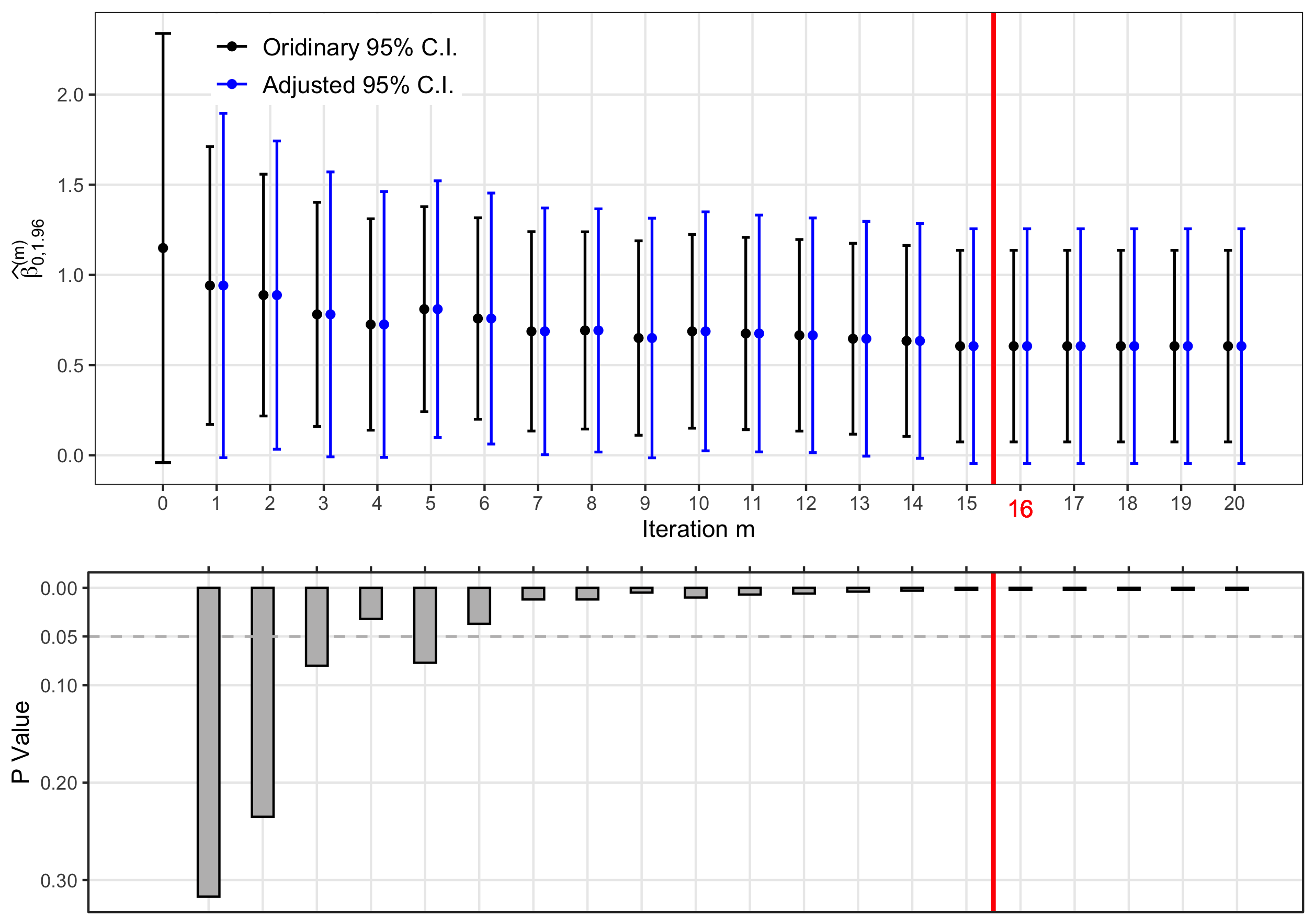
Refer to caption
Figure 5.1: Estimated IV regression coefficients on democracy and the Hausman-type test results over iterations with the chosen cut-off value 1.961.96. The upper panel reports point estimates, ordinary (black) and adjusted (blue) 95%95\% confidence intervals. The lower panel reports p-values of the tests of comparing between the full-sample and the outlier removal estimators. The iterated procedure converges at the iteration step 1616.

By only computing point estimates β~\widetilde{\beta}, β^1.96(1)\widehat{\beta}_{1.96}^{(1)}, β^1.96(∗)\widehat{\beta}_{1.96}^{(\ast)} for the OLS or 2SLS fixed effect regressions without applying formal statistical tests of outlier robustness, we cannot draw any conclusion on whether or not the empirical findings are driven by outliers, since the information contained in the standard errors also needs to be considered in order to evaluate the distance between ordinary and robust estimates. For either the simple regression in Table 5.1 or IVs specification in Table 5.2, both of the heuristic and Hausman tests reject the null hypothesis that the parameter vector β\beta estimated by β~\widetilde{\beta} is identical to the robust estimate β^1.96(1)\widehat{\beta}_{1.96}^{(1)} or β^1.96(∗)\widehat{\beta}_{1.96}^{(\ast)}. It is obvious to note from Columns 4−74-7 in Tables 5.1 and 5.2 that the Hausman tests yield strictly the lower p-values than the heuristic tests, which is concordant with our theory in §3.6 that the Hausman test has the better power performance than the heuristics. In the simple regressions, the Hausman tests reject the null of outlier robustness at the 5%5\% significance level for most coefficients except β2\beta_{2}, β3\beta_{3} when compare β~\widetilde{\beta} with β^1.96(1)\widehat{\beta}_{1.96}^{(1)}; except β3\beta_{3} when compare β~\widetilde{\beta} with β^1.96(∗)\widehat{\beta}_{1.96}^{(\ast)}. In the IVs regressions, the Hausman tests mostly give the same result but the identity of β0\beta_{0} is not rejected by comparing β~\widetilde{\beta} with β^1.96(1)\widehat{\beta}_{1.96}^{(1)}.

Est. Std. Err.(A) 95%95\% Confidence Interval(A) P-value(A)
OLS β~0\widetilde{\beta}_{0} 0.7870.787 0.2280.228 [0.339,1.234][0.339,1.234] 0.0010.001
β^0,1.96(1)\widehat{\beta}_{0,1.96}^{(1)} 0.5560.556 0.150​(0.186)0.150(0.186) [0.262,0.850]​([0.191,0.920])[0.262,0.850]([0.191,0.920]) 0.000​(0.003)0.000(0.003)
β^0,1.96(∗)\widehat{\beta}_{0,1.96}^{(\ast)} 0.1420.142 0.106​(0.129)0.106(0.129) [−0.064,0.349]​([−0.111,0.396])[-0.064,0.349]([-0.111,0.396]) 0.177​(0.271)0.177(0.271)
2SLS β~0\widetilde{\beta}_{0} 1.1491.149 0.6070.607 [−0.041,2.340][-0.041,2.340] 0.0580.058
β^0,1.96(1)\widehat{\beta}_{0,1.96}^{(1)} 0.9410.941 0.393​(0.487)0.393(0.487) [0.170,1.712]​([−0.014,1.897])[0.170,1.712]([-0.014,1.897]) 0.017​(0.054)0.017(0.054)
β^0,1.96(∗)\widehat{\beta}_{0,1.96}^{(\ast)} 0.6050.605 0.271​(0.332)0.271(0.332) [0.074,1.136]​([−0.046,1.257])[0.074,1.136]([-0.046,1.257]) 0.025​(0.069)0.025(0.069)
Table 5.3: This table concentrates on β0\beta_{0} the effect of democracy on log GDP per capita. We present estimates of β0\beta_{0}, standard errors, 95%95\% confidence intervals, and p-values of the tt-test for the null hypothesis β0=0\beta_{0}=0. To compare standard errors and inference with and without the adjustments, we first report the ordinary standard errors and inference, followed by in parentheses ()() the ones adjusted by the theory in §3.5. Rows 1−31-3 represent OLS fixed effect regressions and Rows 4−64-6 2SLS fixed effect regressions. The cut-off is chosen as c=1.96c=1.96, then Algorithm 2.2 is iterated at the step m=−1m=-1, m=0m=0, m=∞m=\infty to produce three estimates β~0\widetilde{\beta}_{0}, β^0,1.96(1)\widehat{\beta}_{0,1.96}^{(1)}, β^0,1.96(∗)\widehat{\beta}_{0,1.96}^{(\ast)} of β0\beta_{0} in simple or IVs regressions. In Row 11 we show the baseline full sample ordinary least squares, and instrument democracy in Row 44. In Row 22 we remove observations with a standardized residual estimated above 1.96 or below -1.96, and the same outlier selection is based on residuals in the second stage in Row 55. In Rows 33 and 66 we iterate the above procedure until reaching the fixed point.

Kaji (2018) also re-examines outlier robustness of the results found in Acemoglu et al. (2019). Without the weak limit of the Hausman type test statistics derived in our paper, he carries out the non-parametric bootstrap to draw the distribution of the L1L_{1} norm of the difference between the baseline full sample estimate and the robust estimate. The bootstrap is implemented by randomly sampling countries ii with replacement. Each draw of country ii adds its time dimensional number of observations to the bootstrap sample. The bootstrap consists of 1000010000 iterations. By comparing between the baseline OLS estimate β~\widetilde{\beta} and outlier-removed estimate β^1.96(1)\widehat{\beta}_{1.96}^{(1)}, the bootstrap does not reject the null that two estimates are identical, indicating robustness to outliers of the empirical findings in Acemoglu et al. (2019). The reason why the null of outlier robustness is not rejected by Kaji (2018) could be the low power issue faced by the bootstrap under alternatives; see discussion in the last paragraph in §3.6. Note that Kaji (2018) only applies the tests for checking the difference for each coefficient β0,β1,…,β4\beta_{0},\beta_{1},\ldots,\beta_{4}, but not for the whole vector β\beta.

Figure 5.1 plots the estimated IV regression results on democracy over iterations (with the cut-off value 1.961.96). The upper panel reports the point estimates, the ordinary and adjusted 95%95\% confidence intervals. The lower panel reports the p-values of the Hausman-type tests of comparing between the full-sample and outlier removal estimates. The red line shows that the iterated procedure converges at the iteration step 1616. We can find that the p-values of the tests become smaller (lower than the conventional level 0.050.05) with increasing iterations. It indicates that we should reply on the trimmed estimates to conduct inference. The outlier removal estimates become closer to zero and the adjusted 95%95\% confidence intervals contain zero for large iteration numbers.

Table 5.3 focuses on β0\beta_{0} the effect of democracy on log GDP per capita by summarizing regression results from Tables 5.1 and 5.2. We present estimates of β0\beta_{0} and compare standard errors with and without the adjustments together with their corresponding inference including 95%95\% confidence intervals and p-values of the tt-test for the null hypothesis that β0=0\beta_{0}=0. The adjusted standard errors and inference results are reported in parentheses ()() after the ordinary ones.

We see from Table 5.3 that the modified standard errors are uniformly larger than those without taking the adjustments, so the adjusted confidence bands are uniformly wider and p-values are uniformly larger; see the theory in §3.5. Recall that the baseline full sample and robust estimates of β0\beta_{0} are statistically different, indicated by the Hausman tests. In the OLS regressions, inference based on β^0,1.96(∗)\widehat{\beta}_{0,1.96}^{(\ast)} shows that β0\beta_{0} is not significantly distinct from 0. In the 2SLS regressions, we cannot reject β0=0\beta_{0}=0 at the 5%5\% significance level by performing the adjusted inference either based on the baseline estimate β~\widetilde{\beta} or the robust estimates β^0,1.96(1)\widehat{\beta}_{0,1.96}^{(1)} and β^0,1.96(∗)\widehat{\beta}_{0,1.96}^{(\ast)}. Thus, we cannot find the evidence robustly supporting the result β0>0\beta_{0}>0 that the effect of democracy is strictly positive on economic growth.

6 Weighted and marked empirical process

Consider the weighted and marked empirical distribution function

𝖥^u,nw,p​(a,b,c)=1n​∑i=1nwi​n​uip​1(ui≤σ​c+n−1/2​a​c+zi​n′​Π​b+n−1/2​ri′​b),\widehat{\mathsf{F}}_{u,n}^{w,p}(a,b,c)=\frac{1}{n}\sum_{i=1}^{n}w_{in}u_{i}^{p}1_{(u_{i}\leq\sigma c+n^{-1/2}ac+z_{in}^{\prime}\Pi b+n^{-1/2}r_{i}^{\prime}b)}, (6.1)

with ℱi−1\mathcal{F}_{i-1} adapted weights wi​nw_{in} and ℱi\mathcal{F}_{i} measurable marks uipu_{i}^{p}. The filtration ℱi−1\mathcal{F}_{i-1} is generated by (z1,…,zi,r1,…,ri−1,u1,…,ui−1)(z_{1},\ldots,z_{i},r_{1},\ldots,r_{i-1},u_{1},\ldots,u_{i-1}) so zi​n∈ℱi−1z_{in}\in\mathcal{F}_{i-1} while ui,ri∈ℱiu_{i},r_{i}\in\mathcal{F}_{i} are independent of ℱi−1\mathcal{F}_{i-1}. The observable data {(yi,xi,zi)}i=1n\{(y_{i},x_{i},z_{i})\}_{i=1}^{n} has i.i.d. structure in this paper, so a∈ℝa\in\mathbb{R}, b∈ℝdxb\in\mathbb{R}^{d_{x}} represent normalized estimation errors a~=n1/2​(σ~−σ)\widetilde{a}=n^{1/2}(\widetilde{\sigma}-\sigma), b~=n1/2​(β~−β)\widetilde{b}=n^{1/2}(\widetilde{\beta}-\beta), and c∈ℝc\in\mathbb{R} is the quantile, while σ\sigma, Π\Pi, Σ\Sigma are true parameters for the variance of the structural error, for the location coefficient in the first stage regression, and for the variance of the first stage error respectively. Let normalized instruments zi​n=n−1/2​ziz_{in}=n^{-1/2}z_{i} such that Mz​z,n=∑i=1nzi​n​zi​n′=n−1​∑i=1nzi​zi′M_{zz,n}=\sum_{i=1}^{n}z_{in}z_{in}^{\prime}=n^{-1}\sum_{i=1}^{n}z_{i}z_{i}^{\prime} converges in probability to 𝖤​zi​zi′=Mz​z\mathsf{E}z_{i}z_{i}^{\prime}=M_{zz} by Law of Large Numbers when 𝖤​|zi|2<∞\mathsf{E}|z_{i}|^{2}<\infty. Our interest focuses on weights wi​nw_{in} given as either of 11, n1/2​zi​n=zin^{1/2}z_{in}=z_{i}, n​zi​n​zi​n′=zi​zi′nz_{in}z_{in}^{\prime}=z_{i}z_{i}^{\prime} and pp as either of 0, 11, 22. To form the empirical process, introduce the compensator

𝖥¯u,nw,p​(a,b,c)=1n​∑i=1nwi​n​𝖤i−1​uip​1(ui≤σ​c+n−1/2​a​c+zi​n′​Π​b+n−1/2​ri′​b),\overline{\mathsf{F}}_{u,n}^{w,p}(a,b,c)=\frac{1}{n}\sum_{i=1}^{n}w_{in}\mathsf{E}_{i-1}u_{i}^{p}1_{(u_{i}\leq\sigma c+n^{-1/2}ac+z_{in}^{\prime}\Pi b+n^{-1/2}r_{i}^{\prime}b)}, (6.2)

where 𝖤i−1(⋅)=𝖤(⋅|ℱi−1)\mathsf{E}_{i-1}(\cdot)=\mathsf{E}(\cdot|\mathcal{F}_{i-1}). Note that 𝖥¯u,n1,0​(0,0,c)=𝖥u​(c)=𝖯​(ui≤σ​c)\overline{\mathsf{F}}_{u,n}^{1,0}(0,0,c)=\mathsf{F}_{u}(c)=\mathsf{P}(u_{i}\leq\sigma c).

We embed these processes into the space D​[0,1]D[0,1] that are processes continuous from the right and with limits of left, where the space is endowed with the Skorokhod metric. We do this as follows. The indicator 1(ui≤σ​c)1_{(u_{i}\leq\sigma c)} and the distribution function 𝖥u​(c)\mathsf{F}_{u}(c) can be defined as 0 or 1 when cc takes the values −∞-\infty and ∞\infty respectively. We can then define quantiles cψ=𝖥u−1​(ψ)c_{\psi}=\mathsf{F}_{u}^{-1}(\psi) for 0≤ψ≤10\leq\psi\leq 1. Correspondingly we can continously extend the definition of the weighted and marked empirical distribution function and its compensator by chosing 𝖥^u,nw,p​(a,b,−∞)=𝖥¯u,nw,p​(a,b,−∞)=0\widehat{\mathsf{F}}_{u,n}^{w,p}(a,b,-\infty)=\overline{\mathsf{F}}_{u,n}^{w,p}(a,b,-\infty)=0 while we then have 𝖥^u,nw,p​(a,b,∞)=n−1​∑i=1nwi​n​uip\widehat{\mathsf{F}}_{u,n}^{w,p}(a,b,\infty)=n^{-1}\sum_{i=1}^{n}w_{in}u_{i}^{p} and 𝖥¯u,nw,p​(a,b,∞)=n−1​∑i=1nwi​n​𝖤i−1​uip\overline{\mathsf{F}}_{u,n}^{w,p}(a,b,\infty)=n^{-1}\sum_{i=1}^{n}w_{in}\mathsf{E}_{i-1}u_{i}^{p}. We now define the empirical process for 0≤ψ≤10\leq\psi\leq 1

𝔽u,nw,p​(a,b,cψ)=n1/2​{𝖥^u,nw,p​(a,b,cψ)−𝖥¯u,nw,p​(a,b,cψ)}.\mathbb{F}_{u,n}^{w,p}(a,b,c_{\psi})=n^{1/2}\{\widehat{\mathsf{F}}_{u,n}^{w,p}(a,b,c_{\psi})-\overline{\mathsf{F}}_{u,n}^{w,p}(a,b,c_{\psi})\}. (6.3)

In the following we first present assumptions, and then results follow for the one-sided process and finally extend to the absolute case.

6.1 Assumptions

In this section, the density 𝖿u\mathsf{f}_{u} is not necessarily symmetric. The conditions listed below are weaker than Assumption 3.1.

Assumption 6.1.

Let ℱi−1=σ​(z1,…,zi,r1,…,ri−1,u1,…,ui−1)\mathcal{F}_{i-1}=\sigma(z_{1},\ldots,z_{i},r_{1},\ldots,r_{i-1},u_{1},\ldots,u_{i-1}) be an increasing sequence of σ\sigma-fields so ui−1u_{i-1}, ri−1r_{i-1}, ziz_{i}, wi​nw_{in} are ℱi−1\mathcal{F}_{i-1} measurable while rir_{i}, uiu_{i} are independent of ℱi−1\mathcal{F}_{i-1}. Suppose (ui/σ,Σ−1/2​ri)(u_{i}/\sigma,\Sigma^{-1/2}r_{i}) have continuously differentiable joint, conditional, and marginal densities 𝖿u,r​(y,x)=𝖿u|r​(y|x)​𝖿r​(x)=𝖿r|u​(x|y)​𝖿u​(y)\mathsf{f}_{u,r}(y,x)=\mathsf{f}_{u|r}(y|x)\mathsf{f}_{r}(x)=\mathsf{f}_{r|u}(x|y)\mathsf{f}_{u}(y) which are positive on y∈ℝy\in\mathbb{R}, x∈ℝdxx\in\mathbb{R}^{d_{x}}. Let p,η,κp,\eta,\kappa be given so p∈ℕ0p\in\mathbb{N}_{0}, 0≤κ<η≤1/40\leq\kappa<\eta\leq 1/4. Choose 0<ν≤10<\nu\leq 1, s∈ℕ0s\in\mathbb{N}_{0} such that

2s−1>1+(1/4−η)​(1+dx).2^{s-1}>1+(1/4-\eta)(1+d_{x}). (6.4)

Suppose
(i)(i) the marginal density 𝖿u​(y)\mathsf{f}_{u}(y) satisfies for y∈ℝy\in\mathbb{R}
(a)(a) moments: ∫−∞∞|y|2s​p/ν​𝖿u​(y)​𝑑y<∞\int_{-\infty}^{\infty}|y|^{2^{s}p/\nu}\mathsf{f}_{u}(y)dy<\infty;
(b)(b) boundedness: supy∈ℝ|y2s​p+1​𝖿u​(y)+y2s​p+2​𝖿˙u​(y)|<∞\sup_{y\in\mathbb{R}}|y^{2^{s}p+1}\mathsf{f}_{u}(y)+y^{2^{s}p+2}\dot{\mathsf{f}}_{u}(y)|<\infty;
(c)(c) smoothness: a CH∈ℕC_{\mathrm{H}}\in\mathbb{N} exists so that for all ϵ>0\epsilon>0

supy≥ϵ(1+y2s​p)​𝖿u​(y)inf0≤y≤ϵ(1+y2s​p)​𝖿u​(y)≤CH,supy≤−ϵ(1+y2s​p)​𝖿u​(y)inf−ϵ≤y≤0(1+y2s​p)​𝖿u​(y)≤CH;\frac{\sup_{y\geq\epsilon}(1+y^{2^{s}p})\mathsf{f}_{u}(y)}{\inf_{0\leq y\leq\epsilon}(1+y^{2^{s}p})\mathsf{f}_{u}(y)}\leq C_{\mathrm{H}},\qquad\frac{\sup_{y\leq-\epsilon}(1+y^{2^{s}p})\mathsf{f}_{u}(y)}{\inf_{-\epsilon\leq y\leq 0}(1+y^{2^{s}p})\mathsf{f}_{u}(y)}\leq C_{\mathrm{H}};

(i​i)(ii) the marginal density 𝖿r​(x)\mathsf{f}_{r}(x) satisfies for x∈ℝdxx\in\mathbb{R}^{d_{x}}
(a)(a) moments: ∫x∈ℝdx|x|4​𝖿r​(x)​(d​x)<∞\int_{x\in\mathbb{R}^{d_{x}}}|x|^{4}\mathsf{f}_{r}(x)(dx)<\infty;
(i​i​i)(iii) the joint and conditional densities 𝖿u,r​(y,x),𝖿u|r​(y|x)\mathsf{f}_{u,r}(y,x),\mathsf{f}_{u|r}(y|x) satisfy for y∈ℝ,x∈ℝdxy\in\mathbb{R},x\in\mathbb{R}^{d_{x}}
(a)(a) boundedness: supy∈ℝ,x∈ℝdx|(1+y)y2s​p−1𝖿u|r(y|x)+y2s​p𝖿˙u|r,y(y|x)|<∞\sup_{y\in\mathbb{R},x\in\mathbb{R}^{d_{x}}}|(1+y)y^{2^{s}p-1}\mathsf{f}_{u|r}(y|x)+y^{2^{s}p}\dot{\mathsf{f}}_{u|r,y}(y|x)|<\infty;
(i​v)(iv) the instruments ziz_{i} satisfy
(a)(a) max1≤i≤n⁡|n1/2−κ​zi​n|=O𝖯​(1)\max_{1\leq i\leq n}|n^{1/2-\kappa}z_{in}|=\mathrm{O}_{\mathsf{P}}(1);
(v)(v) the weights wi​nw_{in} satisfy
(a)(a) n−1​𝖤​∑i=1n|wi​n|2s​(1+|n1/2​zi​n|)=O​(1)n^{-1}\mathsf{E}\sum_{i=1}^{n}|w_{in}|^{2^{s}}(1+|n^{1/2}z_{in}|)=\mathrm{O}(1);
(b)(b) n−1​∑i=1n|wi​n|​(1+|n1/2​zi​n|2)=O𝖯​(1)n^{-1}\sum_{i=1}^{n}|w_{in}|(1+|n^{1/2}z_{in}|^{2})=\mathrm{O}_{\mathsf{P}}(1).

Remark 6.1.

Assumption 3.1(i​a,i​i​a,i​i​i​a,i​v​b,i​v​c)(ia,iia,iiia,ivb,ivc) implies Assumption 6.1 with s≥2s\geq 2 satisfying (6.4) when wi​nw_{in} is either of 11, n1/2​zi​n=zin^{1/2}z_{in}=z_{i}, n​zi​n​zi​n′=zi​zi′nz_{in}z_{in}^{\prime}=z_{i}z_{i}^{\prime} and pp is either of 0, 11, 22. Details are given in Lemma B.1 in the appendix.

6.2 Asymptotic results for empirical process

We present three asymptotic results. The first theorem shows that the estimation error for the scale and regression parameters is negligible uniformly in the quantile.

Theorem 6.1.

Let cψ=𝖥u−1​(ψ)c_{\psi}=\mathsf{F}_{u}^{-1}(\psi). Suppose Assumption 6.1 holds with ν=1\nu=1 and s≥2s\geq 2 satisfying (6.4). Then for any B>0B>0 and as n→∞n\to\infty

sup0≤ψ≤1sup|a|,|b|≤n1/4−η​B|𝔽u,nw,p​(a,b,cψ)−𝔽u,nw,p​(0,0,cψ)|=o𝖯​(1).\sup_{0\leq\psi\leq 1}\sup_{|a|,|b|\leq n^{1/4-\eta}B}|\mathbb{F}_{u,n}^{w,p}(a,b,c_{\psi})-\mathbb{F}_{u,n}^{w,p}(0,0,c_{\psi})|=\mathrm{o}_{\mathsf{P}}(1).

The proof involves a chaining argument. For this, we apply an iterated martingale inequality, see Lemma A.4, to explore the tail behaviour of the maximum of a family of martingales. We can, however, split this argument into two parts. First, we keep bb fixed and consider variation in a,cψa,c_{\psi}. Then we keep aa fixed and consider variation in b,cψb,c_{\psi}. Combining these two arguments will finally finish the proof.

The second result provides a linearization of the compensator.

Theorem 6.2.

Let cψ=𝖥u−1​(ψ)c_{\psi}=\mathsf{F}_{u}^{-1}(\psi). Suppose Assumption 6.1(i​a,i​b,i​i​a,i​i​i​a,v​b)(ia,ib,iia,iiia,vb) holds with ν=1\nu=1, s=0s=0. Then for any B>0B>0 and as n→∞n\to\infty

sup0≤ψ≤1sup|a|,|b|≤n1/4−η​B|n1/2​{𝖥¯u,nw,p​(a,b,cψ)−𝖥¯u,nw,p​(0,0,cψ)}−ℬ𝖥u,n​(a,b,cψ)|=O𝖯​(n−2​η),\sup_{0\leq\psi\leq 1}\sup_{|a|,|b|\leq n^{1/4-\eta}B}|n^{1/2}\{\overline{\mathsf{F}}_{u,n}^{w,p}(a,b,c_{\psi})-\overline{\mathsf{F}}_{u,n}^{w,p}(0,0,c_{\psi})\}-\mathcal{B}_{\mathsf{F}_{u},n}(a,b,c_{\psi})|=\mathrm{O}_{\mathsf{P}}(n^{-2\eta}),

where the bias term, with ξcψ=𝖤​(Σ−1/2​ri|ui/σ=cψ)\xi_{c_{\psi}}=\mathsf{E}(\Sigma^{-1/2}r_{i}|u_{i}/\sigma=c_{\psi}), is defined as

ℬ𝖥u,n​(a,b,cψ)=σp−1​cψp​𝖿u​(cψ)​n−1/2​∑i=1nwi​n​(n−1/2​a​cψ+n−1/2​ξcψ′​Σ1/2​b+zi​n′​Π​b).\mathcal{B}_{\mathsf{F}_{u},n}(a,b,c_{\psi})=\sigma^{p-1}c_{\psi}^{p}\mathsf{f}_{u}(c_{\psi})n^{-1/2}\sum_{i=1}^{n}w_{in}(n^{-1/2}ac_{\psi}+n^{-1/2}\xi_{c_{\psi}}^{\prime}\Sigma^{1/2}b+z_{in}^{\prime}\Pi b).

Since xix_{i} and uiu_{i} are correlated so for uiu_{i} and rir_{i}, this dependent structure requires a more intricate analysis for the compensator. Similar as the proof for uniform convergence in Theorem 6.1, we proceed by first considering variation in a,cψa,c_{\psi} while b=0b=0. We then approximate the compensator by combining with the argument for variation in b,cψb,c_{\psi} while a=0a=0.

Finally, we argue the empirical process 𝔽u,nw,p​(0,0,cψ)\mathbb{F}_{u,n}^{w,p}(0,0,c_{\psi}) is tight when viewed as a sequence in nn of processes on D​[0,1]D[0,1]. By Billingsley (1968, Theorem 13.2), two conditions need to be checked. First, it holds by construction that 𝔽u,nw,p​(0,0,c0)=0\mathbb{F}_{u,n}^{w,p}(0,0,c_{0})=0 where c0=𝖥u−1​(0)=−∞c_{0}=\mathsf{F}_{u}^{-1}(0)=-\infty. Second, the next theorem shows that the modulus of continuity is small. The proof uses a dyadic argument and then apply an iterated martingale exponential inequality, see Lemma A.5, to explore the tail probability of the maximum of a family of martingales.

Theorem 6.3.

Let cψ=𝖥u−1​(ψ)c_{\psi}=\mathsf{F}_{u}^{-1}(\psi). Suppose Assumption 6.1(i​a,v​a)(ia,va) holds with 0<ν<10<\nu<1, s=2s=2. Then for all ϵ>0\epsilon>0

limϕ↓0lim supn→∞𝖯​{sup0≤ψ≤ψ†≤1:ψ†−ψ≤ϕ|𝔽u,nw,p​(0,0,cψ†)−𝔽u,nw,p​(0,0,cψ)|>ϵ}→0.\lim_{\phi\downarrow 0}\limsup_{n\to\infty}\mathsf{P}\{\sup_{0\leq\psi\leq\psi^{\dagger}\leq 1:\psi^{\dagger}-\psi\leq\phi}|\mathbb{F}_{u,n}^{w,p}(0,0,c_{\psi^{\dagger}})-\mathbb{F}_{u,n}^{w,p}(0,0,c_{\psi})|>\epsilon\}\to 0.

The empirical distribution functions 𝖥^u,nw,p​(a,b,c)\widehat{\mathsf{F}}_{u,n}^{w,p}(a,b,c) and Π^c(m+1)\widehat{\Pi}_{c}^{(m+1)} involve in the updated estimators β^c(m+1)\widehat{\beta}_{c}^{(m+1)}, (σ^c(m+1))2(\widehat{\sigma}_{c}^{(m+1)})^{2}, see (2.13), (2.14). While n1/2n^{1/2}-convergence results have been established for the empirical process n1/2​𝖥^u,nw,p​(a,b,c)n^{1/2}\widehat{\mathsf{F}}_{u,n}^{w,p}(a,b,c) by Theorem 6.1, 6.2, 6.3, consistency for the estimator of Π\Pi is then required to build up the asymptotic distribution theory for the iterated estimators of β\beta, σ2\sigma^{2}. A product moment appearing in Π^c(m+1)\widehat{\Pi}_{c}^{(m+1)} but not included in 𝖥^u,nw,p​(a,b,c)\widehat{\mathsf{F}}_{u,n}^{w,p}(a,b,c) is n−1​∑i=1nzi​ri′​vi,c(m)n^{-1}\sum_{i=1}^{n}z_{i}r_{i}^{\prime}v_{i,c}^{(m)}, see (2.11), (2.12). Thus, proving consistency of the Π\Pi estimator, we need the following nn-convergence theorem for a new class of empirical processes with the weight n1/2​zi​n=zin^{1/2}z_{in}=z_{i} and mark ri′r_{i}^{\prime} instead of mark uiu_{i} in the previous case.

Theorem 6.4.

Let cψ=𝖥u−1​(ψ)c_{\psi}=\mathsf{F}_{u}^{-1}(\psi). Suppose Assumption 6.1 holds with ν=1\nu=1 and s≥2s\geq 2 satisfying (6.4). Then for any B>0B>0 and as n→∞n\to\infty

sup0≤ψ≤1sup|a|,|b|≤n1/4−η​B|n−1/2​∑i=1nzi​n​ri′​{1(ui≤σ​cψ+n−1/2​a​cψ+zi​n′​Π​b+n−1/2​ri′​b)−1(ui≤σ​cψ)}|=o𝖯​(1).\sup_{0\leq\psi\leq 1}\sup_{|a|,|b|\leq n^{1/4-\eta}B}|n^{-1/2}\sum_{i=1}^{n}z_{in}r_{i}^{\prime}\{1_{(u_{i}\leq\sigma c_{\psi}+n^{-1/2}ac_{\psi}+z_{in}^{\prime}\Pi b+n^{-1/2}r_{i}^{\prime}b)}-1_{(u_{i}\leq\sigma c_{\psi})}\}|=\mathrm{o}_{\mathsf{P}}(1).

The proof first considers uniform convergence for the empirical process without weights n1/2​zi​n=zin^{1/2}z_{in}=z_{i} and marks rir_{i}. Since we establish nn-convergence result instead of with the normalization n1/2n^{1/2}, the Hölder inequality is then used to prove Theorem 6.4 by adding the weights and marks into the process with only indicators.

6.3 A result for the two-sided empirical process

Estimators in Algorithm 2.1, 2.2, 2.3 involves indicators depending on the absolute value of residuals of structural errors. We therefore present some results for a class of two-sided weighted and marked empirical processes.

Define the weighted and marked absolute empirical distribution function

𝖦^u,nw,p​(a,b,c)=1n​∑i=1nwi​n​uip​1(|ui−zi​n′​Π​b−n−1/2​ri′​b|≤σ​c+n−1/2​a​c).\widehat{\mathsf{G}}_{u,n}^{w,p}(a,b,c)=\frac{1}{n}\sum_{i=1}^{n}w_{in}u_{i}^{p}1_{(|u_{i}-z_{in}^{\prime}\Pi b-n^{-1/2}r_{i}^{\prime}b|\leq\sigma c+n^{-1/2}ac)}. (6.5)

We suppose aa such that σ+n−1/2​a>0\sigma+n^{-1/2}a>0, in which case it suffices to consider c≥0c\geq 0. This restriction on aa is satisfied when choosing aa as a~=n1/2​(σ~−σ)\widetilde{a}=n^{1/2}(\widetilde{\sigma}-\sigma) so that σ+n−1/2​a~=σ~>0\sigma+n^{-1/2}\widetilde{a}=\widetilde{\sigma}>0. Introduce the compensator of 𝖦^u,nw,p​(a,b,c)\widehat{\mathsf{G}}_{u,n}^{w,p}(a,b,c)

𝖦¯u,nw,p​(a,b,c)=1n​∑i=1nwi​n​𝖤i−1​uip​1(|ui−zi​n′​Π​b−n−1/2​ri′​b|≤σ​c+n−1/2​a​c).\overline{\mathsf{G}}_{u,n}^{w,p}(a,b,c)=\frac{1}{n}\sum_{i=1}^{n}w_{in}\mathsf{E}_{i-1}u_{i}^{p}1_{(|u_{i}-z_{in}^{\prime}\Pi b-n^{-1/2}r_{i}^{\prime}b|\leq\sigma c+n^{-1/2}ac)}. (6.6)

Note that 𝖦¯u,n1,0​(0,0,c)=𝖦u​(c)=𝖯​(|ui|≤σ​c)\overline{\mathsf{G}}_{u,n}^{1,0}(0,0,c)=\mathsf{G}_{u}(c)=\mathsf{P}(|u_{i}|\leq\sigma c). Similar as defining the one-sided empirical process 𝔽u,nw,p​(a,b,cψ)\mathbb{F}_{u,n}^{w,p}(a,b,c_{\psi}) on the space D​[0,1]D[0,1] equipped with the Skorokhod metric, let cψ=𝖦u−1​(ψ)c_{\psi}=\mathsf{G}_{u}^{-1}(\psi) for 0≤ψ≤10\leq\psi\leq 1 so cψ≥0c_{\psi}\geq 0 and the absolute empirical process is

𝔾u,nw,p​(a,b,cψ)=n1/2​{𝖦^u,nw,p​(a,b,cψ)−𝖦¯u,nw,p​(a,b,cψ)}.\mathbb{G}_{u,n}^{w,p}(a,b,c_{\psi})=n^{1/2}\{\widehat{\mathsf{G}}_{u,n}^{w,p}(a,b,c_{\psi})-\overline{\mathsf{G}}_{u,n}^{w,p}(a,b,c_{\psi})\}. (6.7)

We can now derive asymptotic theory for the absolute empirical process from Theorems 6.1, 6.2, 6.3, 6.4. These results are presented under more restrictive Assumption 3.1, where the distribution 𝖿u\mathsf{f}_{u} of structural error is symmetric, see Remark 6.1. In this section, we only consider wi​nw_{in} chosen as 11, n1/2​zi​n=zin^{1/2}z_{in}=z_{i}, n​zi​n​zi​n′=zi​zi′nz_{in}z_{in}^{\prime}=z_{i}z_{i}^{\prime} and pp as 0, 11, 22.

The first theorem states the absolute processes with estimation errors converge to the one without estimation errors uniformly in the quantile.

Theorem 6.5.

Let cψ=𝖦u−1​(ψ)c_{\psi}=\mathsf{G}_{u}^{-1}(\psi). Suppose Assumption 3.1(i​a,i​i​a,i​i​i​a,i​v​b,i​v​c)(ia,iia,iiia,ivb,ivc) holds. Then for any B>0B>0 and as n→∞n\to\infty

sup0≤ψ≤1sup|a|,|b|≤n1/4−η​B|𝔾u,nw,p​(a,b,cψ)−𝔾u,nw,p​(0,0,cψ)|=o𝖯​(1).\sup_{0\leq\psi\leq 1}\sup_{|a|,|b|\leq n^{1/4-\eta}B}|\mathbb{G}_{u,n}^{w,p}(a,b,c_{\psi})-\mathbb{G}_{u,n}^{w,p}(0,0,c_{\psi})|=\mathrm{o}_{\mathsf{P}}(1).

Then we provide the first-order approximation to the absolute compensator.

Theorem 6.6.

Let cψ=𝖦u−1​(ψ)c_{\psi}=\mathsf{G}_{u}^{-1}(\psi). Suppose Assumption 3.1(i​a,i​i​a,i​i​i​a,i​v​c)(ia,iia,iiia,ivc) holds. Then for any B>0B>0 and as n→∞n\to\infty

sup0≤ψ≤1sup|a|,|b|≤n1/4−η​B|n1/2​{𝖦¯u,nw,p​(a,b,cψ)−𝖦¯u,nw,p​(0,0,cψ)}−ℬ𝖦u,n​(a,b,cψ)|=O𝖯​(n−2​η),\sup_{0\leq\psi\leq 1}\sup_{|a|,|b|\leq n^{1/4-\eta}B}|n^{1/2}\{\overline{\mathsf{G}}_{u,n}^{w,p}(a,b,c_{\psi})-\overline{\mathsf{G}}_{u,n}^{w,p}(0,0,c_{\psi})\}-\mathcal{B}_{\mathsf{G}_{u},n}(a,b,c_{\psi})|=\mathrm{O}_{\mathsf{P}}(n^{-2\eta}),

where the bias term, with ξcψ=𝖤​(Σ−1/2​ri|ui/σ=cψ)\xi_{c_{\psi}}=\mathsf{E}(\Sigma^{-1/2}r_{i}|u_{i}/\sigma=c_{\psi}), is defined as

ℬ𝖦u,n​(a,b,cψ)\displaystyle\mathcal{B}_{\mathsf{G}_{u},n}(a,b,c_{\psi}) =σp−1cψp𝖿u(cψ)n−1/2∑i=1nwi​n[{1+(−1)p}n−1/2acψ\displaystyle=\sigma^{p-1}c_{\psi}^{p}\mathsf{f}_{u}(c_{\psi})n^{-1/2}\sum_{i=1}^{n}w_{in}[\{1+(-1)^{p}\}n^{-1/2}ac_{\psi}
+n−1/2{ξcψ−(−1)pξ−cψ}′Σ1/2b+{1−(−1)p}zi​n′Πb].\displaystyle\quad\,\,+n^{-1/2}\{\xi_{c_{\psi}}-(-1)^{p}\xi_{-c_{\psi}}\}^{\prime}\Sigma^{1/2}b+\{1-(-1)^{p}\}z_{in}^{\prime}\Pi b].

The next theorem extends the tightness result to the case of empirical processes with absolute indicators.

Theorem 6.7.

Let cψ=𝖦u−1​(ψ)c_{\psi}=\mathsf{G}_{u}^{-1}(\psi). Suppose Assumption 3.1(i​a,i​v​c)(ia,ivc) holds. Then for all ϵ>0\epsilon>0

limϕ↓0lim supn→∞𝖯​{sup0≤ψ≤ψ†≤1:ψ†−ψ≤ϕ|𝔾u,nw,p​(0,0,cψ†)−𝔾u,nw,p​(0,0,cψ)|>ϵ}→0.\lim_{\phi\downarrow 0}\limsup_{n\to\infty}\mathsf{P}\{\sup_{0\leq\psi\leq\psi^{\dagger}\leq 1:\psi^{\dagger}-\psi\leq\phi}|\mathbb{G}_{u,n}^{w,p}(0,0,c_{\psi^{\dagger}})-\mathbb{G}_{u,n}^{w,p}(0,0,c_{\psi})|>\epsilon\}\to 0.

While the above theorems deal with n1/2n^{1/2}-convergence results, the final result considers nn-convergence for a new type of absolute processes used to prove consistency of the estimator for Π\Pi in the first stage regression (2.2).

Theorem 6.8.

Let cψ=𝖦u−1​(ψ)c_{\psi}=\mathsf{G}_{u}^{-1}(\psi). Suppose Assumption 3.1(i​a,i​i​a,i​i​i​a,i​v​b,i​v​c)(ia,iia,iiia,ivb,ivc) holds. Then for any B>0B>0 and as n→∞n\to\infty

sup0≤ψ≤1sup|a|,|b|≤n1/4−η​B|n−1/2​∑i=1nzi​n​ri′​{1(|ui−zi​n′​Π​b−n−1/2​ri′​b|≤σ​cψ+n−1/2​a​cψ)−1(|ui|≤σ​cψ)}|=o𝖯​(1).\sup_{0\leq\psi\leq 1}\sup_{|a|,|b|\leq n^{1/4-\eta}B}|n^{-1/2}\sum_{i=1}^{n}z_{in}r_{i}^{\prime}\{1_{(|u_{i}-z_{in}^{\prime}\Pi b-n^{-1/2}r_{i}^{\prime}b|\leq\sigma c_{\psi}+n^{-1/2}ac_{\psi})}-1_{(|u_{i}|\leq\sigma c_{\psi})}\}|=\mathrm{o}_{\mathsf{P}}(1).

The proofs of empirical processes are given in Appendix B, but first we discuss a metric on ℝ\mathbb{R} and provide some useful inequalities applied repeatedly in the chaining argument in Appendix A. Finally, the proofs of the main results follow in Appendix C.

7 Conclusion and discussion

Since most empirical analyses are affected by atypical observations, when many applied economists apply IVs regressions they first run ordinary 2SLS and use the resulting residuals to find non-outlying observations. They then re-run 2SLS on this subset, subsequently iterating this procedure until they obtain robust results.

In this paper we analyze this simple robust algorithm asymptotically, and provide the consistent estimation and valid inferential procedures given the cut-off value. We concentrate on cross-sectional i.i.d. data in this paper, though our analysis can be extended to time series, whether stationary, deterministic trend, or unit root. The results are all derived under the null hypothesis that there are no outliers in the model. Since in this case there is still a positive probability to find outliers using such algorithms, we then propose the concept of gauge - the expected retention rate of falsely discovered outliers - to evaluate their performance.

Future work should focus on building asymptotic theory for the gauge, to give empirical researchers an indirect way of choosing the cut-off. Furthermore, some specification tests could be devised to check whether outliers truly exist with respect to the reference model (2.1, 2.2), as in Jiao and Pretis (2018).

It is well known that the first order asymptotic approximation is fragile in some small finite sample situations. Therefore, it would be of interest to carry out simulation studies to evaluate the finite sample performance of the results in this paper. Likewise it would be of interest to extend these results to situations where outliers are actually present in the data generating process. Possible scenarios include single outliers, clusters of outliers, level shifts, symmetric or non-symmetric outliers. In such situations, we would analyze the potency, which is the retention rate for relevant outliers.

Appendix A A metric on ℝ\mathbb{R} and some inequalities

The asymptotic theory uses a chaining argument. This involves a partitioning of the quantile axis using a metric, which is presented first. Then follows some preliminary inequalities including an iterated exponential martingale inequality.

For x,y∈ℝx,y\in\mathbb{R} define the function

Ji,p​(x,y)=(uiσ)p​{1(ui/σ≤y)−1(ui/σ≤x)}.J_{i,p}(x,y)=(\frac{u_{i}}{\sigma})^{p}\{1_{(u_{i}/\sigma\leq y)}-1_{(u_{i}/\sigma\leq x)}\}. (A.1)

Our interest focus on Ji,p​(x,y)J_{i,p}(x,y) of order 2s2^{s} with s∈ℕs\in\mathbb{N}. For y,z∈ℝy,z\in\mathbb{R} note z2s​pz^{2^{s}p} is non-negative since 2s​p2^{s}p is even for p∈ℕ0p\in\mathbb{N}_{0} and s∈ℕs\in\mathbb{N}, so introduce a positive and increasing function

𝖧s​(y)=∫−∞y(1+z2s​p)​𝖿u​(z)​𝑑z.\mathsf{H}_{s}(y)=\int_{-\infty}^{y}(1+z^{2^{s}p})\mathsf{f}_{u}(z)dz. (A.2)

The derivative of this function is 𝖧˙s​(y)=(1+y2s​p)​𝖿u​(y)\dot{\mathsf{H}}_{s}(y)=(1+y^{2^{s}p})\mathsf{f}_{u}(y). Then, denote the constant

Hs=𝖧s​(∞)=∫−∞∞(1+z2s​p)​𝖿u​(z)​𝑑z,H_{s}=\mathsf{H}_{s}(\infty)=\int_{-\infty}^{\infty}(1+z^{2^{s}p})\mathsf{f}_{u}(z)dz, (A.3)

which is assumed to be finite. Selection of the specific s∈ℕs\in\mathbb{N} will be more clear in proofs of the empirical process results. The intuition of 𝖧s​(y)\mathsf{H}_{s}(y) is obtained through setting p=0p=0 so that 𝖧s​(y)=2​𝖥u​(y)\mathsf{H}_{s}(y)=2\mathsf{F}_{u}(y), 𝖧˙s​(y)=2​𝖿u​(y)\dot{\mathsf{H}}_{s}(y)=2\mathsf{f}_{u}(y) and Hs=2H_{s}=2. Therefore, 𝖧s​(y)\mathsf{H}_{s}(y) is the generalization of the distribution 𝖥u​(y)∼ui/σ\mathsf{F}_{u}(y)\sim u_{i}/\sigma. Define the metric 𝖽\mathsf{d} on x,y∈ℝx,y\in\mathbb{R} as

𝖽​(x,y)=|𝖧s​(x)−𝖧s​(y)|.\mathsf{d}(x,y)=|\mathsf{H}_{s}(x)-\mathsf{H}_{s}(y)|. (A.4)

Notice the metric 𝖽\mathsf{d} is totally bounded on ℝ\mathbb{R} since 𝖽​(−∞,∞)=Hs<∞\mathsf{d}(-\infty,\infty)=H_{s}<\infty, and it is a special case of the pseudo metric proposed by Koul and Ossiander (1994). For x≤yx\leq y and 1≤q≤s1\leq q\leq s,

0≤𝖤i−1​Ji,p​(x,y)2q=𝖤​Ji,p​(x,y)2q<𝖧s​(y)−𝖧s​(x)=𝖽​(x,y),0\leq\mathsf{E}_{i-1}J_{i,p}(x,y)^{2^{q}}=\mathsf{E}J_{i,p}(x,y)^{2^{q}}<\mathsf{H}_{s}(y)-\mathsf{H}_{s}(x)=\mathsf{d}(x,y), (A.5)

as |z|q<1+|z|s|z|^{q}<1+|z|^{s} for 0≤q≤s0\leq q\leq s.

In the context of chaining, partition the range of 𝖧s​(c)\mathsf{H}_{s}(c) into KK intervals of equal size Hs/KH_{s}/K. In other words, use the metric 𝖽\mathsf{d} to partition ℝ\mathbb{R} into KK intervals by endpoints

−∞=c0<c1<⋯<cK−1<cK=∞,-\infty=c_{0}<c_{1}<\cdots<c_{K-1}<c_{K}=\infty, (A.6)

with c−k=c0c_{-k}=c_{0} for k∈ℕk\in\mathbb{N} so that 𝖽​(ck−1,ck)=Hs/K\mathsf{d}(c_{k-1},c_{k})=H_{s}/K for 1≤k≤K1\leq k\leq K.

We first prove an inequality for the difference of two indicators, which will be used to control variation within the chaining interval.

Lemma A.1.

For any e,e0e,e_{0} on the uu-axis and d≥|e−e0|d\geq|e-e_{0}|, we have an inequality

|1(u≤e)−1(u≤e0)|≤1(e0−d≤u≤e0+d).|1_{(u\leq e)}-1_{(u\leq e_{0})}|\leq 1_{(e_{0}-d\leq u\leq e_{0}+d)}.
Proof of Lemma A.1.

From |e−e0|≤d|e-e_{0}|\leq d we find e0−d≤e≤e0+de_{0}-d\leq e\leq e_{0}+d. Suppose e≥e0e\geq e_{0}, then using the monotonicity of the indicator function in ee and e0e_{0}, we have

|1(u≤e)−1(u≤e0)|=1(e0≤u≤e)≤1(e0−d≤u≤e0+d).|1_{(u\leq e)}-1_{(u\leq e_{0})}|=1_{(e_{0}\leq u\leq e)}\leq 1_{(e_{0}-d\leq u\leq e_{0}+d)}.

The similar argument applies for e<e0e<e_{0}, so we also have

|1(u≤e)−1(u≤e0)|=1(e≤u≤e0)≤1(e0−d≤u≤e0+d).∎|1_{(u\leq e)}-1_{(u\leq e_{0})}|=1_{(e\leq u\leq e_{0})}\leq 1_{(e_{0}-d\leq u\leq e_{0}+d)}.\qed

The next lemma is the bias correction for differences in expectations involving two dependent random variables, which will be used to linearize the compensator.

Lemma A.2.

Let (Y,X)(Y,X) be a random vector with dimension 1+dx1+d_{x} with the joint density 𝗆​(y,x)\mathsf{m}(y,x) for y∈ℝ,x∈ℝdxy\in\mathbb{R},x\in\mathbb{R}^{d_{x}}. Suppose the joint density decomposes into the conditional and marginal densities as 𝗆​(y,x)=𝗆Y|X​(y|x)​𝗆X​(x)=𝗆X|Y​(x|y)​𝗆Y​(y)\mathsf{m}(y,x)=\mathsf{m}_{Y|X}(y|x)\mathsf{m}_{X}(x)=\mathsf{m}_{X|Y}(x|y)\mathsf{m}_{Y}(y) and its derivative for yy exists so 𝗆˙y​(y,x)=𝗆˙Y|X,y​(y|x)​𝗆X​(x)\dot{\mathsf{m}}_{y}(y,x)=\dot{\mathsf{m}}_{Y|X,y}(y|x)\mathsf{m}_{X}(x). Let b1∈ℝb_{1}\in\mathbb{R}, b2∈ℝdxb_{2}\in\mathbb{R}^{d_{x}}, and p∈ℕ0p\in\mathbb{N}_{0}. Assume 𝖤​|X|2<∞\mathsf{E}|X|^{2}<\infty, then

supc∈ℝ|𝖤Yp{1(Y≤c+b1+X′​b2)−1(Y≤c)}−cp𝗆Y(c){b1+𝖤(X′b2|Y=c)}|\displaystyle\sup_{c\in\mathbb{R}}|\mathsf{E}Y^{p}\{1_{(Y\leq c+b_{1}+X^{\prime}b_{2})}-1_{(Y\leq c)}\}-c^{p}\mathsf{m}_{Y}(c)\{b_{1}+\mathsf{E}(X^{\prime}b_{2}|Y=c)\}|
≤\displaystyle\leq (12b12+|b1||b2|𝖤|X|+12|b2|2𝖤|X|2)supy∈ℝ,x∈ℝdx|pyp−1𝗆Y|X(y|x)+yp𝗆˙Y|X,y(y|x)|.\displaystyle(\frac{1}{2}b_{1}^{2}+|b_{1}||b_{2}|\mathsf{E}|X|+\frac{1}{2}|b_{2}|^{2}\mathsf{E}|X|^{2})\sup_{y\in\mathbb{R},x\in\mathbb{R}^{d_{x}}}|py^{p-1}\mathsf{m}_{Y|X}(y|x)+y^{p}\dot{\mathsf{m}}_{Y|X,y}(y|x)|.
Proof of Lemma A.2.

Let ℰ=𝖤​Yp​{1(Y≤c+b1+X′​b2)−1(Y≤c)}\mathcal{E}=\mathsf{E}Y^{p}\{1_{(Y\leq c+b_{1}+X^{\prime}b_{2})}-1_{(Y\leq c)}\}, and write the expectation as an integral

ℰ=∬y∈ℝ,x∈ℝdxyp​1(c≤y≤c+b1+x′​b2)​𝗆​(y,x)​𝑑y​(d​x)=∫x∈ℝdx∫cc+b1+x′​b2yp​𝗆​(y,x)​𝑑y​(d​x).\mathcal{E}=\iint_{y\in\mathbb{R},x\in\mathbb{R}^{d_{x}}}y^{p}1_{(c\leq y\leq c+b_{1}+x^{\prime}b_{2})}\mathsf{m}(y,x)dy(dx)=\int_{x\in\mathbb{R}^{d_{x}}}\int_{c}^{c+b_{1}+x^{\prime}b_{2}}y^{p}\mathsf{m}(y,x)dy(dx).

Apply Taylor expansion at point cc to the inner integral to obtain

∫cc+b1+x′​b2yp​𝗆​(y,x)​𝑑y=(b1+x′​b2)​cp​𝗆​(c,x)+12​(b1+x′​b2)2​{p​c~p−1​𝗆​(c~,x)+c~p​𝗆˙y​(c~,x)},\int_{c}^{c+b_{1}+x^{\prime}b_{2}}y^{p}\mathsf{m}(y,x)dy=(b_{1}+x^{\prime}b_{2})c^{p}\mathsf{m}(c,x)+\frac{1}{2}(b_{1}+x^{\prime}b_{2})^{2}\{p\tilde{c}^{p-1}\mathsf{m}(\tilde{c},x)+\tilde{c}^{p}\dot{\mathsf{m}}_{y}(\tilde{c},x)\},

where |c~−c|≤|b1+x′​b2||\tilde{c}-c|\leq|b_{1}+x^{\prime}b_{2}|. Then ℰ\mathcal{E} is approximated by the first order term ℰ1\mathcal{E}_{1} with the remainder term ℰ2\mathcal{E}_{2} left so ℰ=ℰ1+ℰ2\mathcal{E}=\mathcal{E}_{1}+\mathcal{E}_{2} where

ℰ1\displaystyle\mathcal{E}_{1} =∫ℝdx(b1+x′​b2)​cp​𝗆​(c,x)​(d​x),\displaystyle=\int_{\mathbb{R}^{d_{x}}}(b_{1}+x^{\prime}b_{2})c^{p}\mathsf{m}(c,x)(dx),
ℰ2\displaystyle\mathcal{E}_{2} =12​∫ℝdx(b1+x′​b2)2​{p​c~p−1​𝗆​(c~,x)+c~p​𝗆˙y​(c~,x)}​(d​x).\displaystyle=\frac{1}{2}\int_{\mathbb{R}^{d_{x}}}(b_{1}+x^{\prime}b_{2})^{2}\{p\tilde{c}^{p-1}\mathsf{m}(\tilde{c},x)+\tilde{c}^{p}\dot{\mathsf{m}}_{y}(\tilde{c},x)\}(dx).

Analyze the first order term ℰ1\mathcal{E}_{1} to get

ℰ1=cp​𝗆Y​(c)​b1+cp​𝗆Y​(c)​∫ℝdxx′​b2​𝗆X|Y​(x|c)​(d​x)=cp​𝗆Y​(c)​{b1+𝖤​(X′​b2|Y=c)}.\mathcal{E}_{1}=c^{p}\mathsf{m}_{Y}(c)b_{1}+c^{p}\mathsf{m}_{Y}(c)\int_{\mathbb{R}^{d_{x}}}x^{\prime}b_{2}\mathsf{m}_{X|Y}(x|c)(dx)=c^{p}\mathsf{m}_{Y}(c)\{b_{1}+\mathsf{E}(X^{\prime}b_{2}|Y=c)\}.

For the remainder term ℰ2=ℰ−ℰ1\mathcal{E}_{2}=\mathcal{E}-\mathcal{E}_{1}, apply the triangle inequality so

|ℰ2|≤12∫ℝdx{b12+2|b1x′b2|+(x′b2)2}|pc~p−1𝗆Y|X(c~|x)+c~p𝗆˙Y|X,y(c~|x)|𝗆X(x)(dx).|\mathcal{E}_{2}|\leq\frac{1}{2}\int_{\mathbb{R}^{d_{x}}}\{b_{1}^{2}+2|b_{1}x^{\prime}b_{2}|+(x^{\prime}b_{2})^{2}\}|p\tilde{c}^{p-1}\mathsf{m}_{Y|X}(\tilde{c}|x)+\tilde{c}^{p}\dot{\mathsf{m}}_{Y|X,y}(\tilde{c}|x)|\mathsf{m}_{X}(x)(dx).

As |b1​x′​b2|≤|b1|​|b2|​|x||b_{1}x^{\prime}b_{2}|\leq|b_{1}||b_{2}||x| and (x′​b2)2≤|x|2​|b2|2(x^{\prime}b_{2})^{2}\leq|x|^{2}|b_{2}|^{2}, so

|ℰ2|≤(12b12+|b1||b2|𝖤|X|+12|b2|2𝖤|X|2)supy∈ℝ,x∈ℝdx|pyp−1𝗆Y|X(y|x)+yp𝗆˙Y|X,y(y|x)|.∎|\mathcal{E}_{2}|\leq(\frac{1}{2}b_{1}^{2}+|b_{1}||b_{2}|\mathsf{E}|X|+\frac{1}{2}|b_{2}|^{2}\mathsf{E}|X|^{2})\sup_{y\in\mathbb{R},x\in\mathbb{R}^{d_{x}}}|py^{p-1}\mathsf{m}_{Y|X}(y|x)+y^{p}\dot{\mathsf{m}}_{Y|X,y}(y|x)|.\qed

The next inequality provides a tightness type result for the metric 𝖽\mathsf{d}, which will be used to prove the tightness property of empirical process 𝔽u,nw,p​(0,0,cψ)\mathbb{F}_{u,n}^{w,p}(0,0,c_{\psi}).

Lemma A.3.

(Johansen and Nielsen, 2016a, Lemma B.3). Let cψ=𝖥u−1​(ψ)c_{\psi}=\mathsf{F}_{u}^{-1}(\psi). Suppose Assumption 6.1(i​a)(ia) holds with 0<ν<10<\nu<1, s∈ℕ0s\in\mathbb{N}_{0}. Then there exist CνC_{\nu}, 0<ϕ0<10<\phi_{0}<1 so that for 0≤ϕ≤ϕ00\leq\phi\leq\phi_{0} it follows sup0≤ψ≤1−ϕ𝖽​(cψ,cψ+ϕ)≤Cν​ϕ1−ν\sup_{0\leq\psi\leq 1-\phi}\mathsf{d}(c_{\psi},c_{\psi+\phi})\leq C_{\nu}\phi^{1-\nu}.

The chaining argument involves the tail behaviour of the maximum of a family of martingales which can be controlled using the iterated exponential martingale inequality from Johansen and Nielsen (2016a). It builds on an exponential martingale inequality derived by Bercu and Touati (2008, Theorem 2.1) which relaxes the need of boundedness for martingale difference series but required in Freedman (1975) inequality. The following are two special cases of iterated exponential martingale inequalities, where the number of elements in the martingale family is increasing and where it is fixed. The first inequality will be used to demonstrate the uniform convergence result for empirical processes, while the second is for handling the tightness property.

Lemma A.4.

(Johansen and Nielsen, 2016a, Theorem 5.2) For ll so 1≤l≤L1\leq l\leq L, let zl,iz_{l,i} be ℱi\mathcal{F}_{i} adapted satisfying 𝖤​zl,i2s<∞\mathsf{E}z_{l,i}^{2^{s}}<\infty for some s∈ℕs\in\mathbb{N}. Let Dq=max1≤l≤L​∑i=1n𝖤i−1​zl,i2qD_{q}=\max_{1\leq l\leq L}\sum_{i=1}^{n}\mathsf{E}_{i-1}z_{l,i}^{2^{q}} for 1≤q≤s1\leq q\leq s. Suppose, for some ς≥0\varsigma\geq 0, λ>0\lambda>0, that L=O​(nλ)L=\mathrm{O}(n^{\lambda}) and 𝖤​Dq=O​(nς)\mathsf{E}D_{q}=\mathrm{O}(n^{\varsigma}) for 1≤q≤s1\leq q\leq s. If υ>0\upsilon>0 is chosen such that
(i)(i) ς<2​υ\varsigma<2\upsilon;
(i​i)(ii) ς+λ<υ​2s\varsigma+\lambda<\upsilon 2^{s};
then, we have for all κ>0\kappa>0

limn→∞𝖯​{max1≤l≤L⁡|∑i=1n(zl,i−𝖤i−1​zl,i)|>κ​nυ}=0.\lim_{n\to\infty}\mathsf{P}\{\max_{1\leq l\leq L}|\sum_{i=1}^{n}{(z_{l,i}-\mathsf{E}_{i-1}z_{l,i})}|>\kappa n^{\upsilon}\}=0.
Lemma A.5.

(Johansen and Nielsen, 2016a, Theorem 5.3) For ll so 1≤l≤L1\leq l\leq L, let zl,iz_{l,i} be ℱi\mathcal{F}_{i} adapted satisfying 𝖤​zl,i4<∞\mathsf{E}z_{l,i}^{4}<\infty. Let Dq=max1≤l≤L​∑i=1n𝖤i−1​zl,i2qD_{q}=\max_{1\leq l\leq L}\sum_{i=1}^{n}\mathsf{E}_{i-1}z_{l,i}^{2^{q}} and suppose 𝖤​Dq≤D​n\mathsf{E}D_{q}\leq Dn for q=1,2q=1,2 and some D>0D>0. Then for all θ,κ>0\theta,\kappa>0

𝖯​{max1≤l≤L⁡|∑i=1n(zl,i−𝖤i−1​zl,i)|>κ​n1/2}≤(L+1)​θ3​Dκ​n+θ​Dκ+4​L​exp⁡(−κ​θ14).\mathsf{P}\{\max_{1\leq l\leq L}|\sum_{i=1}^{n}{(z_{l,i}-\mathsf{E}_{i-1}z_{l,i})}|>\kappa n^{1/2}\}\leq\frac{(L+1)\theta^{3}D}{\kappa n}+\frac{\theta D}{\kappa}+4L\exp(-\frac{\kappa\theta}{14}).

Appendix B Proofs of the empirical process results

We first prove uniform n1/2n^{1/2}-convergence and tightness for the one-sided empirical processes, then linearize the compensator term and show nn-convergence for a specific type of the process. Finally, extend all results to the processes considering absolute residuals.

B.1 Uniform n1/2n^{1/2}-convergence of empirical process

We first consider Theorem B.1 which allows variation in a,ba,b but cc fixed. Then use the argument in Johansen and Nielsen (2016b, Theorem 4.1) to extend the result to Theorem B.2 where we have variation in b,cb,c but a=0a=0, also see Berenguer-Rico, Johansen, and Nielsen (2019a, Theorem 3.1), while use Jiao and Nielsen (2017, Theorem 5) to prove Theorem B.3 showing convergence uniformly in a,ca,c but b=0b=0. Finally, by combining Theorem B.2, B.3 the uniform convergence in a,b,ca,b,c follows.

Theorem B.1.

Let cψ=𝖥u−1​(ψ)c_{\psi}=\mathsf{F}_{u}^{-1}(\psi). Suppose Assumption 6.1(i​a,i​i​a,i​i​i​a,v)(ia,iia,iiia,v) holds with ν=1\nu=1 and s≥1s\geq 1 such that 2s−1>1/2+(1/4−η)​(2+dx)2^{s-1}>1/2+(1/4-\eta)(2+d_{x}). Then for any 0≤ψ≤10\leq\psi\leq 1, B>0B>0 and as n→∞n\to\infty

sup|a|,|b|≤n1/4−η​B|𝔽u,nw,p​(a,b,cψ)−𝔽u,nw,p​(0,0,cψ)|=o𝖯​(1).\sup_{|a|,|b|\leq n^{1/4-\eta}B}|\mathbb{F}_{u,n}^{w,p}(a,b,c_{\psi})-\mathbb{F}_{u,n}^{w,p}(0,0,c_{\psi})|=\mathrm{o}_{\mathsf{P}}(1).
Proof of Theorem B.1.

Without loss of generality let σ=1\sigma=1, Σ1/2=Idx\Sigma^{1/2}=I_{d_{x}}. Denote Rn​(a,b,cψ)=𝔽u,nw,p​(a,b,cψ)−𝔽u,nw,p​(0,0,cψ)R_{n}(a,b,c_{\psi})=\mathbb{F}_{u,n}^{w,p}(a,b,c_{\psi})-\mathbb{F}_{u,n}^{w,p}(0,0,c_{\psi}) so we want to show ℛψ,n=o𝖯​(1)\mathcal{R}_{\psi,n}=\mathrm{o}_{\mathsf{P}}(1) for any 0≤ψ≤10\leq\psi\leq 1 as n→∞n\to\infty where ℛψ,n=sup|a|,|b|≤n1/4−η​B|Rn​(a,b,cψ)|\mathcal{R}_{\psi,n}=\sup_{|a|,|b|\leq n^{1/4-\eta}B}|R_{n}(a,b,c_{\psi})|. Throughout denote C>0C>0 as usual a constant which may have different values in different expressions.

11. Construct a,ba,b-balls. For δ,n>0\delta,n>0, cover the set |a|,|b|≤n1/4−η​B|a|,|b|\leq n^{1/4-\eta}B with balls of radius δ\delta and centers aj,bma_{j},b_{m}. The numbers of a,ba,b-balls are J=n1/4−η​B/δ=O​(n1/4−η/δ)J=n^{1/4-\eta}B/\delta=\mathrm{O}(n^{1/4-\eta}/\delta) and M=(n1/4−η​B/δ)dx=O​(n(1/4−η)​dx/δ)M=(n^{1/4-\eta}B/\delta)^{d_{x}}=\mathrm{O}(n^{(1/4-\eta)d_{x}}/\delta) respectively. Thus, for any a,ba,b there exist aj,bma_{j},b_{m} so that |a−aj|≤δ|a-a_{j}|\leq\delta and |b−bm|≤δ|b-b_{m}|\leq\delta.

22. Apply chaining. Write Rn​(a,b,cψ)=Rn​(aj,bm,cψ)+{Rn​(a,b,cψ)−Rn​(aj,bm,cψ)}R_{n}(a,b,c_{\psi})=R_{n}(a_{j},b_{m},c_{\psi})+\{R_{n}(a,b,c_{\psi})-R_{n}(a_{j},b_{m},c_{\psi})\} where Rn​(aj,bm,cψ)R_{n}(a_{j},b_{m},c_{\psi}) is a discrete point term while Rn​(a,b,cψ)−Rn​(aj,bm,cψ)R_{n}(a,b,c_{\psi})-R_{n}(a_{j},b_{m},c_{\psi}) is a local oscillation term. The triangle inequality gives ℛψ,n≤ℛψ,n,1+ℛψ,n,2\mathcal{R}_{\psi,n}\leq\mathcal{R}_{\psi,n,1}+\mathcal{R}_{\psi,n,2} where

ℛψ,n,1\displaystyle\mathcal{R}_{\psi,n,1} =max1≤j≤J,1≤m≤M⁡|Rn​(aj,bm,cψ)|,\displaystyle=\max_{1\leq j\leq J,1\leq m\leq M}|R_{n}(a_{j},b_{m},c_{\psi})|,
ℛψ,n,2\displaystyle\mathcal{R}_{\psi,n,2} =max1≤j≤J,1≤m≤M​sup|a−aj|≤δ,|b−bm|≤δ|Rn​(a,b,cψ)−Rn​(aj,bm,cψ)|.\displaystyle=\max_{1\leq j\leq J,1\leq m\leq M}\sup_{|a-a_{j}|\leq\delta,|b-b_{m}|\leq\delta}|R_{n}(a,b,c_{\psi})-R_{n}(a_{j},b_{m},c_{\psi})|.

It then suffices to show that ℛψ,n,1,ℛψ,n,2\mathcal{R}_{\psi,n,1},\mathcal{R}_{\psi,n,2} are o𝖯​(1)\mathrm{o}_{\mathsf{P}}(1).

33. The discrete point term ℛψ,n,1\mathcal{R}_{\psi,n,1} is o𝖯​(1)\mathrm{o}_{\mathsf{P}}(1). Recall the notation Ji,pJ_{i,p} in (A.1), then write Rn​(aj,bm,cψ)=n−1/2​∑i=1n(zl,i−𝖤i−1​zl,i)R_{n}(a_{j},b_{m},c_{\psi})=n^{-1/2}\sum_{i=1}^{n}(z_{l,i}-\mathsf{E}_{i-1}z_{l,i}) where

zl,i=wi​n​Ji,p​(cψ,cψ+n−1/2​aj​cψ+zi​n′​Π​bm+n−1/2​ri′​bm).z_{l,i}=w_{in}J_{i,p}(c_{\psi},c_{\psi}+n^{-1/2}a_{j}c_{\psi}+z_{in}^{\prime}\Pi b_{m}+n^{-1/2}r_{i}^{\prime}b_{m}).

Use Lemma A.4 with υ=1/2\upsilon=1/2, index l=(j,m)l=(j,m) and L=J​ML=JM to prove ℛψ,n,1=o𝖯​(1)\mathcal{R}_{\psi,n,1}=\mathrm{o}_{\mathsf{P}}(1), and we need to verify its conditions.

The moment 𝖤​zl,i2s<∞\mathsf{E}z_{l,i}^{2^{s}}<\infty for s∈ℕs\in\mathbb{N}. Bounding the difference of indicator functions by unity and using independence of uiu_{i} with ℱi−1\mathcal{F}_{i-1} gives 𝖤​zl,i2s≤𝖤​|wi​n|2s​ui2s​p=𝖤​|wi​n|2s​𝖤​ui2s​p\mathsf{E}z_{l,i}^{2^{s}}\leq\mathsf{E}|w_{in}|^{2^{s}}u_{i}^{2^{s}p}=\mathsf{E}|w_{in}|^{2^{s}}\mathsf{E}u_{i}^{2^{s}p}. This is finite by Assumption 6.1(i​a,v​a)(ia,va).

The parameter λ\lambda. The set of indices ll has the size L=J​ML=JM. Since J=O​(n1/4−η/δ)J=\mathrm{O}(n^{1/4-\eta}/\delta) and M=O​(n(1/4−η)​dx/δ)M=\mathrm{O}(n^{(1/4-\eta)d_{x}}/\delta) while δ\delta is now treated as a constant then L=O​(nλ)L=\mathrm{O}(n^{\lambda}) where λ=(1/4−η)​(1+dx)\lambda=(1/4-\eta)(1+d_{x}).

The parameter ς\varsigma. Consider 1≤q≤s1\leq q\leq s. Notice we have

|1(ui≤cψ+n−1/2​aj​cψ+zi​n′​Π​bm+n−1/2​ri′​bm)−1(ui≤cψ)|≤1(c¯i​ψ​j​m,ri≤ui≤c¯i​ψ​j​m,ri),|1_{(u_{i}\leq c_{\psi}+n^{-1/2}a_{j}c_{\psi}+z_{in}^{\prime}\Pi b_{m}+n^{-1/2}r_{i}^{\prime}b_{m})}-1_{(u_{i}\leq c_{\psi})}|\leq 1_{(\underline{c}_{i\psi jm,r_{i}}\leq u_{i}\leq\overline{c}_{i\psi jm,r_{i}})},

where we denote

c¯i​ψ​j​m,ri\displaystyle\underline{c}_{i\psi jm,r_{i}} =cψ−n−1/2​|aj|​|cψ|−|zi​n|​|Π|​|bm|−n−1/2​|ri|​|bm|,\displaystyle=c_{\psi}-n^{-1/2}|a_{j}||c_{\psi}|-|z_{in}||\Pi||b_{m}|-n^{-1/2}|r_{i}||b_{m}|,
c¯i​ψ​j​m,ri\displaystyle\overline{c}_{i\psi jm,r_{i}} =cψ+n−1/2​|aj|​|cψ|+|zi​n|​|Π|​|bm|+n−1/2​|ri|​|bm|.\displaystyle=c_{\psi}+n^{-1/2}|a_{j}||c_{\psi}|+|z_{in}||\Pi||b_{m}|+n^{-1/2}|r_{i}||b_{m}|.

The above follows from Lemma A.1 by e=cψ+n−1/2​aj​cψ+zi​n′​Π​bm+n−1/2​ri′​bme=c_{\psi}+n^{-1/2}a_{j}c_{\psi}+z_{in}^{\prime}\Pi b_{m}+n^{-1/2}r_{i}^{\prime}b_{m}, e0=cψe_{0}=c_{\psi}, d=n−1/2​|aj|​|cψ|+|zi​n|​|Π|​|bm|+n−1/2​|ri|​|bm|≥|n−1/2​aj​cψ+zi​n′​Π​bm+n−1/2​ri′​bm|=|e−e0|d=n^{-1/2}|a_{j}||c_{\psi}|+|z_{in}||\Pi||b_{m}|+n^{-1/2}|r_{i}||b_{m}|\geq|n^{-1/2}a_{j}c_{\psi}+z_{in}^{\prime}\Pi b_{m}+n^{-1/2}r_{i}^{\prime}b_{m}|=|e-e_{0}|. Let ℰi=𝖤i−1​Ji,p2q​(cψ,cψ+n−1/2​aj​cψ+zi​n′​Π​bm+n−1/2​ri′​bm)\mathcal{E}_{i}=\mathsf{E}_{i-1}J_{i,p}^{2^{q}}(c_{\psi},c_{\psi}+n^{-1/2}a_{j}c_{\psi}+z_{in}^{\prime}\Pi b_{m}+n^{-1/2}r_{i}^{\prime}b_{m}), then by applying the above inequality concerning the difference of indicator functions we have

ℰi≤𝖤i−1​Ji,p2q​(c¯i​ψ​j​m,ri,c¯i​ψ​j​m,ri)=∬y∈ℝ,x∈ℝdxy2q​p​1(c¯i​ψ​j​m,x≤y≤c¯i​ψ​j​m,x)​𝖿u,r​(y,x)​𝑑y​(d​x).\mathcal{E}_{i}\leq\mathsf{E}_{i-1}J_{i,p}^{2^{q}}(\underline{c}_{i\psi jm,r_{i}},\overline{c}_{i\psi jm,r_{i}})=\iint_{y\in\mathbb{R},x\in\mathbb{R}^{d_{x}}}y^{2^{q}p}1_{(\underline{c}_{i\psi jm,x}\leq y\leq\overline{c}_{i\psi jm,x})}\mathsf{f}_{u,r}(y,x)dy(dx).

Decompose the joint density into the conditional and marginal ones, then apply the mean value theorem to the inner integral to get

ℰi\displaystyle\mathcal{E}_{i} ≤∫x∈ℝdx{∫c¯i​ψ​j​m,xc¯i​ψ​j​m,x(1+y2s​p)​𝖿u|r​(y|x)​𝑑y}​𝖿r​(x)​(d​x)\displaystyle\leq\int_{x\in\mathbb{R}^{d_{x}}}\{\int_{\underline{c}_{i\psi jm,x}}^{\overline{c}_{i\psi jm,x}}(1+y^{2^{s}p})\mathsf{f}_{u|r}(y|x)dy\}\mathsf{f}_{r}(x)(dx)
=∫x∈ℝdx(c¯i​ψ​j​m,x−c¯i​ψ​j​m,x)​(1+c~2s​p)​𝖿u|r​(c~|x)​𝖿r​(x)​(d​x),\displaystyle=\int_{x\in\mathbb{R}^{d_{x}}}(\overline{c}_{i\psi jm,x}-\underline{c}_{i\psi jm,x})(1+\tilde{c}^{2^{s}p})\mathsf{f}_{u|r}(\tilde{c}|x)\mathsf{f}_{r}(x)(dx),

for an intermediate point c~\tilde{c} such that c¯i​ψ​j​m,x≤c~≤c¯i​ψ​j​m,x\underline{c}_{i\psi jm,x}\leq\tilde{c}\leq\overline{c}_{i\psi jm,x}. Insert c¯i​ψ​j​m,x,c¯i​ψ​j​m,x\underline{c}_{i\psi jm,x},\overline{c}_{i\psi jm,x} to get

ℰi≤2​supy∈ℝ,x∈ℝdx(1+y2s​p)​𝖿u|r​(y|x)​∫x∈ℝdxn−1/2​(|aj|​|cψ|+|n1/2​zi​n|​|Π|​|bm|+|x|​|bm|)​𝖿r​(x)​(d​x).\mathcal{E}_{i}\leq 2\sup_{y\in\mathbb{R},x\in\mathbb{R}^{d_{x}}}(1+y^{2^{s}p})\mathsf{f}_{u|r}(y|x)\int_{x\in\mathbb{R}^{d_{x}}}n^{-1/2}(|a_{j}||c_{\psi}|+|n^{1/2}z_{in}||\Pi||b_{m}|+|x||b_{m}|)\mathsf{f}_{r}(x)(dx).

Note |aj|,|bm|≤n1/4−η​B|a_{j}|,|b_{m}|\leq n^{1/4-\eta}B for each 1≤j≤J1\leq j\leq J, 1≤m≤M1\leq m\leq M while cψc_{\psi}, Π\Pi are fixed. Furthermore, since Assumption 6.1(i​i​a,i​i​i​a)(iia,iiia) that ∫x∈ℝdx|x|​𝖿r​(x)​(d​x)<∞\int_{x\in\mathbb{R}^{d_{x}}}|x|\mathsf{f}_{r}(x)(dx)<\infty and that supy∈ℝ,x∈ℝdx(1+y2s​p)​𝖿u|r​(y|x)<∞\sup_{y\in\mathbb{R},x\in\mathbb{R}^{d_{x}}}(1+y^{2^{s}p})\mathsf{f}_{u|r}(y|x)<\infty, then there exists C>0C>0 so uniformly in j,mj,m

ℰi≤C​n−1/4−η​∫x∈ℝdx(1+|n1/2​zi​n|+|x|)​𝖿r​(x)​(d​x)≤C​n−1/4−η​(1+|n1/2​zi​n|).\mathcal{E}_{i}\leq Cn^{-1/4-\eta}\int_{x\in\mathbb{R}^{d_{x}}}(1+|n^{1/2}z_{in}|+|x|)\mathsf{f}_{r}(x)(dx)\leq Cn^{-1/4-\eta}(1+|n^{1/2}z_{in}|).

Insert the bound of ℰi\mathcal{E}_{i} to get

Dq=max1≤l≤L​∑i=1n𝖤i−1​zl,i2q=max1≤j≤J,1≤m≤M​∑i=1n|wi​n|2q​ℰi≤C​n−1/4−η​∑i=1n|wi​n|2q​(1+|n1/2​zi​n|).D_{q}=\max_{1\leq l\leq L}\sum_{i=1}^{n}\mathsf{E}_{i-1}z_{l,i}^{2^{q}}=\max_{1\leq j\leq J,1\leq m\leq M}\sum_{i=1}^{n}|w_{in}|^{2^{q}}\mathcal{E}_{i}\leq Cn^{-1/4-\eta}\sum_{i=1}^{n}|w_{in}|^{2^{q}}(1+|n^{1/2}z_{in}|).

Since |wi​n|2q≤(1+|wi​n|2s)|w_{in}|^{2^{q}}\leq(1+|w_{in}|^{2^{s}}) and 𝖤​∑i=1n(1+|wi​n|2s)​(1+|n1/2​zi​n|)=O​(n)\mathsf{E}\sum_{i=1}^{n}(1+|w_{in}|^{2^{s}})(1+|n^{1/2}z_{in}|)=\mathrm{O}(n) by Assumption 6.1(v​a)(va), then we have 𝖤​Dq=O​(nς)\mathsf{E}D_{q}=\mathrm{O}(n^{\varsigma}) where ς=3/4−η\varsigma=3/4-\eta.

Condition (i)(i) is that ς<2​υ\varsigma<2\upsilon. This holds since η>0\eta>0 so ς=3/4−η<1=2​υ\varsigma=3/4-\eta<1=2\upsilon.

Condition (i​i)(ii) is that ς+λ<υ​2s\varsigma+\lambda<\upsilon 2^{s}. We have

ς+λ=3/4−η+(1/4−η)​(1+dx)=1/2+(1/4−η)​(2+dx).\varsigma+\lambda=3/4-\eta+(1/4-\eta)(1+d_{x})=1/2+(1/4-\eta)(2+d_{x}).

We choose ss so that ς+λ<υ​2s=2s−1\varsigma+\lambda<\upsilon 2^{s}=2^{s-1}.

44. Decompose the oscillation term ℛψ,n,2\mathcal{R}_{\psi,n,2}. As the terms 𝔽u,nw,p​(0,0,cψ)\mathbb{F}_{u,n}^{w,p}(0,0,c_{\psi}) in Rn​(a,b,cψ)R_{n}(a,b,c_{\psi}) and Rn​(aj,bm,cψ)R_{n}(a_{j},b_{m},c_{\psi}) cancel out, then we have

Rn​(a,b,cψ)−Rn​(aj,bm,cψ)=𝔽u,nw,p​(a,b,cψ)−𝔽u,nw,p​(aj,bm,cψ).R_{n}(a,b,c_{\psi})-R_{n}(a_{j},b_{m},c_{\psi})=\mathbb{F}_{u,n}^{w,p}(a,b,c_{\psi})-\mathbb{F}_{u,n}^{w,p}(a_{j},b_{m},c_{\psi}).

Let si,p​(a,aj,b,bm,cψ)s_{i,p}(a,a_{j},b,b_{m},c_{\psi}) denote the term

wi​n​uip​{1(ui≤cψ+n−1/2​a​cψ+zi​n′​Π​b+n−1/2​ri′​b)−1(ui≤cψ+n−1/2​aj​cψ+zi​n′​Π​bm+n−1/2​ri′​bm)},w_{in}u_{i}^{p}\{1_{(u_{i}\leq c_{\psi}+n^{-1/2}ac_{\psi}+z_{in}^{\prime}\Pi b+n^{-1/2}r_{i}^{\prime}b)}-1_{(u_{i}\leq c_{\psi}+n^{-1/2}a_{j}c_{\psi}+z_{in}^{\prime}\Pi b_{m}+n^{-1/2}r_{i}^{\prime}b_{m})}\},

it then follows

Rn​(a,b,cψ)−Rn​(aj,bm,cψ)=n−1/2​∑i=1n{si,p​(a,aj,b,bm,cψ)−𝖤i−1​si,p​(a,aj,b,bm,cψ)}.R_{n}(a,b,c_{\psi})-R_{n}(a_{j},b_{m},c_{\psi})=n^{-1/2}\sum_{i=1}^{n}\{s_{i,p}(a,a_{j},b,b_{m},c_{\psi})-\mathsf{E}_{i-1}s_{i,p}(a,a_{j},b,b_{m},c_{\psi})\}.

Choose e=cψ+n−1/2​a​cψ+zi​n′​Π​b+n−1/2​ri′​be=c_{\psi}+n^{-1/2}ac_{\psi}+z_{in}^{\prime}\Pi b+n^{-1/2}r_{i}^{\prime}b and e0=cψ+n−1/2​aj​cψ+zi​n′​Π​bm+n−1/2​ri′​bme_{0}=c_{\psi}+n^{-1/2}a_{j}c_{\psi}+z_{in}^{\prime}\Pi b_{m}+n^{-1/2}r_{i}^{\prime}b_{m}, then find |e−e0|=|n−1/2​(a−aj)​cψ+zi​n′​Π​(b−bm)+n−1/2​ri′​(b−bm)||e-e_{0}|=|n^{-1/2}(a-a_{j})c_{\psi}+z_{in}^{\prime}\Pi(b-b_{m})+n^{-1/2}r_{i}^{\prime}(b-b_{m})|. For any j,mj,m it holds |a−aj|≤δ|a-a_{j}|\leq\delta, |b−bm|≤δ|b-b_{m}|\leq\delta, so |e−e0|≤n−1/2​δ​(|cψ|+|n1/2​zi​n|​|Π|+|ri|)=d|e-e_{0}|\leq n^{-1/2}\delta(|c_{\psi}|+|n^{1/2}z_{in}||\Pi|+|r_{i}|)=d. Thus, apply Lemma A.1 to bound the difference of two indicators so that

|1(ui≤cψ+n−1/2​a​cψ+zi​n′​Π​b+n−1/2​ri′​b)−1(ui≤cψ+n−1/2​aj​cψ+zi​n′​Π​bm+n−1/2​ri′​bm)|≤1(c¯¯i​ψ​j​m,ri≤ui≤c¯¯i​ψ​j​m,ri),|1_{(u_{i}\leq c_{\psi}+n^{-1/2}ac_{\psi}+z_{in}^{\prime}\Pi b+n^{-1/2}r_{i}^{\prime}b)}-1_{(u_{i}\leq c_{\psi}+n^{-1/2}a_{j}c_{\psi}+z_{in}^{\prime}\Pi b_{m}+n^{-1/2}r_{i}^{\prime}b_{m})}|\leq 1_{(\underline{\underline{c}}_{i\psi jm,r_{i}}\leq u_{i}\leq\overline{\overline{c}}_{i\psi jm,r_{i}})},

where we deonote

c¯¯i​ψ​j​m,ri\displaystyle\underline{\underline{c}}_{i\psi jm,r_{i}} =cψ+n−1/2​aj​cψ+zi​n′​Π​bm+n−1/2​ri′​bm−n−1/2​δ​(|cψ|+|n1/2​zi​n|​|Π|+|ri|),\displaystyle=c_{\psi}+n^{-1/2}a_{j}c_{\psi}+z_{in}^{\prime}\Pi b_{m}+n^{-1/2}r_{i}^{\prime}b_{m}-n^{-1/2}\delta(|c_{\psi}|+|n^{1/2}z_{in}||\Pi|+|r_{i}|),
c¯¯i​ψ​j​m,ri\displaystyle\overline{\overline{c}}_{i\psi jm,r_{i}} =cψ+n−1/2​aj​cψ+zi​n′​Π​bm+n−1/2​ri′​bm+n−1/2​δ​(|cψ|+|n1/2​zi​n|​|Π|+|ri|).\displaystyle=c_{\psi}+n^{-1/2}a_{j}c_{\psi}+z_{in}^{\prime}\Pi b_{m}+n^{-1/2}r_{i}^{\prime}b_{m}+n^{-1/2}\delta(|c_{\psi}|+|n^{1/2}z_{in}||\Pi|+|r_{i}|).

Apply the above inequality to get |si,p​(a,aj,b,bm,cψ)|≤|wi​n|​|Ji,p​(c¯¯i​ψ​j​m,ri,c¯¯i​ψ​j​m,ri)||s_{i,p}(a,a_{j},b,b_{m},c_{\psi})|\leq|w_{in}||J_{i,p}(\underline{\underline{c}}_{i\psi jm,r_{i}},\overline{\overline{c}}_{i\psi jm,r_{i}})|, then it follows by the triangle and Jensen’s inequality that

|Rn​(a,b,cψ)−Rn​(aj,bm,cψ)|\displaystyle|R_{n}(a,b,c_{\psi})-R_{n}(a_{j},b_{m},c_{\psi})|
≤\displaystyle\leq n−1/2​∑i=1n|wi​n|​{|Ji,p​(c¯¯i​ψ​j​m,ri,c¯¯i​ψ​j​m,ri)|+𝖤i−1​|Ji,p​(c¯¯i​ψ​j​m,ri,c¯¯i​ψ​j​m,ri)|}.\displaystyle n^{-1/2}\sum_{i=1}^{n}|w_{in}|\{|J_{i,p}(\underline{\underline{c}}_{i\psi jm,r_{i}},\overline{\overline{c}}_{i\psi jm,r_{i}})|+\mathsf{E}_{i-1}|J_{i,p}(\underline{\underline{c}}_{i\psi jm,r_{i}},\overline{\overline{c}}_{i\psi jm,r_{i}})|\}.

Decompose the oscillation term ℛψ,n,2\mathcal{R}_{\psi,n,2} into a martingale and two compensators such that ℛψ,n,2≤ℛ~ψ,n,2+2​ℛ¯ψ,n,2\mathcal{R}_{\psi,n,2}\leq\widetilde{\mathcal{R}}_{\psi,n,2}+2\overline{\mathcal{R}}_{\psi,n,2}, where

ℛ~ψ,n,2\displaystyle\widetilde{\mathcal{R}}_{\psi,n,2} =max1≤j≤J,1≤m≤M⁡n−1/2​∑i=1n|wi​n|​{|Ji,p​(c¯¯i​ψ​j​m,ri,c¯¯i​ψ​j​m,ri)|−𝖤i−1​|Ji,p​(c¯¯i​ψ​j​m,ri,c¯¯i​ψ​j​m,ri)|}\displaystyle=\max_{1\leq j\leq J,1\leq m\leq M}n^{-1/2}\sum_{i=1}^{n}|w_{in}|\{|J_{i,p}(\underline{\underline{c}}_{i\psi jm,r_{i}},\overline{\overline{c}}_{i\psi jm,r_{i}})|-\mathsf{E}_{i-1}|J_{i,p}(\underline{\underline{c}}_{i\psi jm,r_{i}},\overline{\overline{c}}_{i\psi jm,r_{i}})|\}
ℛ¯ψ,n,2\displaystyle\overline{\mathcal{R}}_{\psi,n,2} =max1≤j≤J,1≤m≤M⁡n−1/2​∑i=1n|wi​n|​𝖤i−1​|Ji,p​(c¯¯i​ψ​j​m,ri,c¯¯i​ψ​j​m,ri)|.\displaystyle=\max_{1\leq j\leq J,1\leq m\leq M}n^{-1/2}\sum_{i=1}^{n}|w_{in}|\mathsf{E}_{i-1}|J_{i,p}(\underline{\underline{c}}_{i\psi jm,r_{i}},\overline{\overline{c}}_{i\psi jm,r_{i}})|.

Thus, it suffices to prove that ℛ~ψ,n,2\widetilde{\mathcal{R}}_{\psi,n,2} and ℛ¯ψ,n,2\overline{\mathcal{R}}_{\psi,n,2} are o𝖯​(1)\mathrm{o}_{\mathsf{P}}(1).

55. Bounding the compensator ℛ¯ψ,n,2\overline{\mathcal{R}}_{\psi,n,2}. Let ℰ¯i=𝖤i−1​|Ji,p​(c¯¯i​ψ​j​m,ri,c¯¯i​ψ​j​m,ri)|\overline{\mathcal{E}}_{i}=\mathsf{E}_{i-1}|J_{i,p}(\underline{\underline{c}}_{i\psi jm,r_{i}},\overline{\overline{c}}_{i\psi jm,r_{i}})|, then it is clear to see ℰ¯i≤ℋi=𝖤i−1​(1+ui2s​p)​1(c¯¯i​ψ​j​m,ri≤ui≤c¯¯i​ψ​j​m,ri)\overline{\mathcal{E}}_{i}\leq\mathcal{H}_{i}=\mathsf{E}_{i-1}(1+u_{i}^{2^{s}p})1_{(\underline{\underline{c}}_{i\psi jm,r_{i}}\leq u_{i}\leq\overline{\overline{c}}_{i\psi jm,r_{i}})} for s≥1s\geq 1, and thus our aim now is to bound ℋi\mathcal{H}_{i}. Write ℋi\mathcal{H}_{i} as an integral and decompose the joint density so that

ℋi\displaystyle\mathcal{H}_{i} =∬y∈ℝ,x∈ℝdx(1+y2s​p)​1(c¯¯i​ψ​j​m,x≤y≤c¯¯i​ψ​j​m,x)​𝖿u,r​(y,x)​𝑑y​(d​x)\displaystyle=\iint_{y\in\mathbb{R},x\in\mathbb{R}^{d_{x}}}(1+y^{2^{s}p})1_{(\underline{\underline{c}}_{i\psi jm,x}\leq y\leq\overline{\overline{c}}_{i\psi jm,x})}\mathsf{f}_{u,r}(y,x)dy(dx)
=∫x∈ℝdx{∫c¯¯i​ψ​j​m,xc¯¯i​ψ​j​m,x(1+y2s​p)​𝖿u|r​(y|x)​𝑑y}​𝖿r​(x)​(d​x).\displaystyle=\int_{x\in\mathbb{R}^{d_{x}}}\{\int_{\underline{\underline{c}}_{i\psi jm,x}}^{\overline{\overline{c}}_{i\psi jm,x}}(1+y^{2^{s}p})\mathsf{f}_{u|r}(y|x)dy\}\mathsf{f}_{r}(x)(dx).

Apply the mean value theorem to the inner integral to get

ℋi=∫x∈ℝdx(c¯¯i​ψ​j​m,x−c¯¯i​ψ​j​m,x)​(1+c~~2s​p)​𝖿u|r​(c~~|x)​𝖿r​(x)​(d​x),\mathcal{H}_{i}=\int_{x\in\mathbb{R}^{d_{x}}}(\overline{\overline{c}}_{i\psi jm,x}-\underline{\underline{c}}_{i\psi jm,x})(1+\tilde{\tilde{c}}^{2^{s}p})\mathsf{f}_{u|r}(\tilde{\tilde{c}}|x)\mathsf{f}_{r}(x)(dx),

where c~~\tilde{\tilde{c}} is an intermediate point so that c¯¯i​ψ​j​m,x≤c~~≤c¯¯i​ψ​j​m,x\underline{\underline{c}}_{i\psi jm,x}\leq\tilde{\tilde{c}}\leq\overline{\overline{c}}_{i\psi jm,x}. Insert c¯¯i​ψ​j​m,x\underline{\underline{c}}_{i\psi jm,x}, c¯¯i​ψ​j​m,x\overline{\overline{c}}_{i\psi jm,x} into ℋi\mathcal{H}_{i} and bound the function (1+y2s​p)​𝖿u|r​(y|x)(1+y^{2^{s}p})\mathsf{f}_{u|r}(y|x), then it follows

ℋi≤2​n−1/2​δ​supy∈ℝ,x∈ℝdx(1+y2s​p)​𝖿u|r​(y|x)​∫x∈ℝdx(|cψ|+|n1/2​zi​n|​|Π|+|x|)​𝖿r​(x)​(d​x).\mathcal{H}_{i}\leq 2n^{-1/2}\delta\sup_{y\in\mathbb{R},x\in\mathbb{R}^{d_{x}}}(1+y^{2^{s}p})\mathsf{f}_{u|r}(y|x)\int_{x\in\mathbb{R}^{d_{x}}}(|c_{\psi}|+|n^{1/2}z_{in}||\Pi|+|x|)\mathsf{f}_{r}(x)(dx).

Due to Assumption 6.1(i​i​a,i​i​i​a)(iia,iiia) and that cψc_{\psi}, Π\Pi are fixed, it holds uniformly in 1≤j≤J1\leq j\leq J, 1≤m≤M1\leq m\leq M that ℋi≤C​n−1/2​δ​(1+|n1/2​zi​n|)\mathcal{H}_{i}\leq Cn^{-1/2}\delta(1+|n^{1/2}z_{in}|). Therefore, recall ℰ¯i≤ℋi\overline{\mathcal{E}}_{i}\leq\mathcal{H}_{i} then we find

ℛ¯ψ,n,2=max1≤j≤J,1≤m≤M⁡n−1/2​∑i=1n|wi​n|​ℰ¯i≤C​n−1/2​δ​n−1/2​∑i=1n|wi​n|​(1+|n1/2​zi​n|).\overline{\mathcal{R}}_{\psi,n,2}=\max_{1\leq j\leq J,1\leq m\leq M}n^{-1/2}\sum_{i=1}^{n}|w_{in}|\overline{\mathcal{E}}_{i}\leq Cn^{-1/2}\delta n^{-1/2}\sum_{i=1}^{n}|w_{in}|(1+|n^{1/2}z_{in}|).

Assumption 6.1(v​b)(vb) that n−1​∑i=1n|wi​n|​(1+|n1/2​zi​n|)=O𝖯​(1)n^{-1}\sum_{i=1}^{n}|w_{in}|(1+|n^{1/2}z_{in}|)=\mathrm{O}_{\mathsf{P}}(1) shows ℛ¯ψ,n,2=δ​O𝖯​(1)\overline{\mathcal{R}}_{\psi,n,2}=\delta\mathrm{O}_{\mathsf{P}}(1), where the O𝖯​(1)\mathrm{O}_{\mathsf{P}}(1)-term does not depend on δ\delta. Choose δ\delta sufficiently small then it follows ℛ¯ψ,n,2=o𝖯​(1)\overline{\mathcal{R}}_{\psi,n,2}=\mathrm{o}_{\mathsf{P}}(1).

66. The martingale ℛ~ψ,n,2\widetilde{\mathcal{R}}_{\psi,n,2} is o𝖯​(1)\mathrm{o}_{\mathsf{P}}(1). Note that once δ\delta is selected in item 55, it is then treated as constant so does not play any particular role in other items. To show ℛ~ψ,n,2=o𝖯​(1)\widetilde{\mathcal{R}}_{\psi,n,2}=\mathrm{o}_{\mathsf{P}}(1), use Lemma A.4 with υ=1/2\upsilon=1/2 and zl,i=|wi​n|​|Ji,p​(c¯¯i​ψ​j​m,ri,c¯¯i​ψ​j​m,ri)|z_{l,i}=|w_{in}||J_{i,p}(\underline{\underline{c}}_{i\psi jm,r_{i}},\overline{\overline{c}}_{i\psi jm,r_{i}})| where the index l=(j,m)l=(j,m) has the size L=J​ML=JM. Two conditions need to shown.

The moment 𝖤​zl,i2s<∞\mathsf{E}z_{l,i}^{2^{s}}<\infty for s∈ℕs\in\mathbb{N}. This can be shown by the same argument used in the item 33.

The parameter λ\lambda. The size L=O​(nλ)L=\mathrm{O}(n^{\lambda}) where λ=(1/4−η)​(1+dx)\lambda=(1/4-\eta)(1+d_{x}), since L=J​ML=JM and J=O​(n1/4−η)J=\mathrm{O}(n^{1/4-\eta}), M=O​(n(1/4−η)​dx)M=\mathrm{O}(n^{(1/4-\eta)d_{x}}).

The parameter ς\varsigma. Consider 1≤q≤s1\leq q\leq s and let ℰ~i=𝖤i−1​Ji,p2q​(c¯¯i​ψ​j​m,ri,c¯¯i​ψ​j​m,ri)\widetilde{\mathcal{E}}_{i}=\mathsf{E}_{i-1}J_{i,p}^{2^{q}}(\underline{\underline{c}}_{i\psi jm,r_{i}},\overline{\overline{c}}_{i\psi jm,r_{i}}). Item 55 shows the bound of ℋi\mathcal{H}_{i}, so we find ℰ~i≤ℋi≤C​n−1/2​(1+|n1/2​zi​n|)\widetilde{\mathcal{E}}_{i}\leq\mathcal{H}_{i}\leq Cn^{-1/2}(1+|n^{1/2}z_{in}|) uniformly in j,mj,m. Insert the bound of ℰ~i\widetilde{\mathcal{E}}_{i} to get

Dq=max1≤l≤L​∑i=1n𝖤i−1​zl,i2q=max1≤j≤J,1≤m≤M​∑i=1n|wi​n|2q​ℰ~i≤C​n−1/2​∑i=1n|wi​n|2q​(1+|n1/2​zi​n|).D_{q}=\max_{1\leq l\leq L}\sum_{i=1}^{n}\mathsf{E}_{i-1}z_{l,i}^{2^{q}}=\max_{1\leq j\leq J,1\leq m\leq M}\sum_{i=1}^{n}|w_{in}|^{2^{q}}\widetilde{\mathcal{E}}_{i}\leq Cn^{-1/2}\sum_{i=1}^{n}|w_{in}|^{2^{q}}(1+|n^{1/2}z_{in}|).

Due to |wi​n|2q≤(1+|wi​n|2s)|w_{in}|^{2^{q}}\leq(1+|w_{in}|^{2^{s}}) and Assumption 6.1(v​a)(va), we have 𝖤​Dq=O​(nς)\mathsf{E}D_{q}=\mathrm{O}(n^{\varsigma}) where ς=1/2\varsigma=1/2.

Condition (i)(i) holds, since ς=1/2<1=2​υ\varsigma=1/2<1=2\upsilon.

Condition (i​i)(ii) holds, since

ς+λ=1/2+(1/4−η)​(1+dx)≤1/2+(1/4−η)​(2+dx)<2s−1=υ​2s.\varsigma+\lambda=1/2+(1/4-\eta)(1+d_{x})\leq 1/2+(1/4-\eta)(2+d_{x})<2^{s-1}=\upsilon 2^{s}.

Notice that the first inequality above is due to η≤1/4\eta\leq 1/4 and the number of moments ss is selected in the item 33 such that 2s−1≥1/2+(1/4−η)​(2+dx)2^{s-1}\geq 1/2+(1/4-\eta)(2+d_{x}). ∎

Theorem B.2.

Let cψ=𝖥u−1​(ψ)c_{\psi}=\mathsf{F}_{u}^{-1}(\psi). Suppose Assumption 6.1(i,i​i​a,i​i​i​a,i​v​a,v​a)(i,iia,iiia,iva,va) holds with ν=1\nu=1 and s≥2s\geq 2 satisfying (6.4). Then for any B>0B>0 and as n→∞n\to\infty

sup0≤ψ≤1sup|b|≤n1/4−η​B|𝔽u,nw,p​(0,b,cψ)−𝔽u,nw,p​(0,0,cψ)|=o𝖯​(1).\sup_{0\leq\psi\leq 1}\sup_{|b|\leq n^{1/4-\eta}B}|\mathbb{F}_{u,n}^{w,p}(0,b,c_{\psi})-\mathbb{F}_{u,n}^{w,p}(0,0,c_{\psi})|=\mathrm{o}_{\mathsf{P}}(1).
Proof of Theorem B.2.

Set a=0a=0 and then apply the argument by Johansen and Nielsen (2016a, Theorem 4.1) and Berenguer-Rico, Johansen, and Nielsen (2019a, Theorem 3.1) to extend pointwise convergence shown in Theorem B.1 to convergence uniformly in ψ\psi. It further requires chaining for the cψc_{\psi}-axis, so for δ,n>0\delta,n>0 use the metric 𝖽\mathsf{d} to partition the quantile axis as laid out in (A.6) with K=int​(Hs​n1/2/δ)K=\mathrm{int}(H_{s}n^{1/2}/\delta) where s≥2s\geq 2 such that (6.4) 2s−1>1+(1/4−η)​(1+dx)2^{s-1}>1+(1/4-\eta)(1+d_{x}) holds. Notice s≥2s\geq 2 satisfying 2s−1>1+(1/4−η)​(1+dx)2^{s-1}>1+(1/4-\eta)(1+d_{x}) implies s≥1s\geq 1 and 2s−1>1/2+(1/4−η)​(2+dx)2^{s-1}>1/2+(1/4-\eta)(2+d_{x}), so we need the higher moment condition on ss for proving the uniform convergence. ∎

Theorem B.3.

Let cψ=𝖥u−1​(ψ)c_{\psi}=\mathsf{F}_{u}^{-1}(\psi). Suppose Assumption 6.1(i​a,i​b,v)(ia,ib,v) holds with ν=1\nu=1, s=2s=2. Then for any B>0B>0 and as n→∞n\to\infty

sup0≤ψ≤1sup|a|≤n1/4−η​B|𝔽u,nw,p​(a,0,cψ)−𝔽u,nw,p​(0,0,cψ)|=o𝖯​(1).\sup_{0\leq\psi\leq 1}\sup_{|a|\leq n^{1/4-\eta}B}|\mathbb{F}_{u,n}^{w,p}(a,0,c_{\psi})-\mathbb{F}_{u,n}^{w,p}(0,0,c_{\psi})|=\mathrm{o}_{\mathsf{P}}(1).
Proof of Theorem B.3.

For δ,n>0\delta,n>0 use the metric 𝖽\mathsf{d} to partition the cψc_{\psi}-axis as laid out in (A.6) with K=int​(Hs​n1/2/δ)K=\mathrm{int}(H_{s}n^{1/2}/\delta) where s=2s=2, then argue as the proof of Theorem 5 in Jiao and Nielsen (2017) to show convergence uniformly in ψ\psi, aa. ∎

Proof of Theorem 6.1.

The term of interest is 𝒲=𝔽u,nw,p​(a,b,cψ)−𝔽u,nw,p​(0,0,cψ)\mathcal{W}=\mathbb{F}_{u,n}^{w,p}(a,b,c_{\psi})-\mathbb{F}_{u,n}^{w,p}(0,0,c_{\psi}). Denote cψ†=cψ​(1+n−1/2​a/σ)c_{\psi^{\dagger}}=c_{\psi}(1+n^{-1/2}a/\sigma). Notice that 𝔽u,nw,p​(a,b,cψ)=𝔽u,nw,p​(0,b,cψ†)\mathbb{F}_{u,n}^{w,p}(a,b,c_{\psi})=\mathbb{F}_{u,n}^{w,p}(0,b,c_{\psi^{\dagger}}) so it follows that 𝒲=𝔽u,nw,p​(0,b,cψ†)−𝔽u,nw,p​(0,0,cψ)\mathcal{W}=\mathbb{F}_{u,n}^{w,p}(0,b,c_{\psi^{\dagger}})-\mathbb{F}_{u,n}^{w,p}(0,0,c_{\psi}). Add and subtract 𝔽u,nw,p​(a,0,cψ)=𝔽u,nw,p​(0,0,cψ†)\mathbb{F}_{u,n}^{w,p}(a,0,c_{\psi})=\mathbb{F}_{u,n}^{w,p}(0,0,c_{\psi^{\dagger}}) and apply the triangle inequality to get

|𝒲|≤|𝔽u,nw,p​(0,b,cψ†)−𝔽u,nw,p​(0,0,cψ†)|+|𝔽u,nw,p​(a,0,cψ)−𝔽u,nw,p​(0,0,cψ)|.|\mathcal{W}|\leq|\mathbb{F}_{u,n}^{w,p}(0,b,c_{\psi^{\dagger}})-\mathbb{F}_{u,n}^{w,p}(0,0,c_{\psi^{\dagger}})|+|\mathbb{F}_{u,n}^{w,p}(a,0,c_{\psi})-\mathbb{F}_{u,n}^{w,p}(0,0,c_{\psi})|.

Thus, the problem reduces to showing

sup0≤ψ†≤1sup|b|≤n1/4−η​B|𝔽u,nw,p​(0,b,cψ†)−𝔽u,nw,p​(0,0,cψ†)|\displaystyle\sup_{0\leq\psi^{\dagger}\leq 1}\sup_{|b|\leq n^{1/4-\eta}B}|\mathbb{F}_{u,n}^{w,p}(0,b,c_{\psi^{\dagger}})-\mathbb{F}_{u,n}^{w,p}(0,0,c_{\psi^{\dagger}})| =o𝖯​(1),\displaystyle=\mathrm{o}_{\mathsf{P}}(1), (B.1)
sup0≤ψ≤1sup|a|≤n1/4−η​B|𝔽u,nw,p​(a,0,cψ)−𝔽u,nw,p​(0,0,cψ)|\displaystyle\sup_{0\leq\psi\leq 1}\sup_{|a|\leq n^{1/4-\eta}B}|\mathbb{F}_{u,n}^{w,p}(a,0,c_{\psi})-\mathbb{F}_{u,n}^{w,p}(0,0,c_{\psi})| =o𝖯​(1).\displaystyle=\mathrm{o}_{\mathsf{P}}(1). (B.2)

Then (B.1) was considered by Theorem B.2 using Assumption 6.1(i,i​i​a,i​i​i​a,i​v​a,v​a)(i,iia,iiia,iva,va) with ν=1\nu=1 and s≥2s\geq 2 such that (6.4) holds. Further, (B.2) follows by Theorem B.3, which requires Assumption 6.1(i​a,i​b,v)(ia,ib,v) with ν=1\nu=1, s=2s=2. ∎

B.2 Linearization of compensator

Theorem 6.2 is proved by further considering two separate cases where variation in a,cψa,c_{\psi} but b=0b=0 and where in b,cψb,c_{\psi} but a=0a=0. The next theorem shows the bias correction term in the first situation where bb is set to 0 and only a,cψa,c_{\psi} vary. The proof has the similar spirit as linearization of compensator in Jiao and Nielsen (2017, Theorem 8).

Theorem B.4.

Let cψ=𝖥u−1​(ψ)c_{\psi}=\mathsf{F}_{u}^{-1}(\psi). Suppose Assumption 6.1(i​a,i​b,v​b)(ia,ib,vb) holds with ν=1\nu=1, s=0s=0. Then for any B>0B>0 and as n→∞n\to\infty

sup0≤ψ≤1sup|a|≤n1/4−η​B|n1/2​{𝖥¯u,nw,p​(a,0,cψ)−𝖥¯u,nw,p​(0,0,cψ)}−ℬ𝖥u,n​(a,0,cψ)|=O𝖯​(n−2​η),\sup_{0\leq\psi\leq 1}\sup_{|a|\leq n^{1/4-\eta}B}|n^{1/2}\{\overline{\mathsf{F}}_{u,n}^{w,p}(a,0,c_{\psi})-\overline{\mathsf{F}}_{u,n}^{w,p}(0,0,c_{\psi})\}-\mathcal{B}_{\mathsf{F}_{u},n}(a,0,c_{\psi})|=\mathrm{O}_{\mathsf{P}}(n^{-2\eta}),

where the bias term is defined as

ℬ𝖥u,n​(a,0,cψ)=σp−1​cψp​𝖿u​(cψ)​n−1/2​∑i=1nwi​n​n−1/2​a​cψ.\mathcal{B}_{\mathsf{F}_{u},n}(a,0,c_{\psi})=\sigma^{p-1}c_{\psi}^{p}\mathsf{f}_{u}(c_{\psi})n^{-1/2}\sum_{i=1}^{n}w_{in}n^{-1/2}ac_{\psi}.
Proof of Theorem B.4.

See the proof of Theorem 8 in Jiao and Nielsen (2017) which is the generalized version of the above theorem, so follow their argument but set b=0b=0 in their context. ∎

We state next theorem to handle variation in b,cψb,c_{\psi} while aa is set to 0.

Theorem B.5.

Let cψ=𝖥u−1​(ψ)c_{\psi}=\mathsf{F}_{u}^{-1}(\psi). Suppose Assumption 6.1(i​a,i​i​a,i​i​i​a,v​b)(ia,iia,iiia,vb) holds with ν=1\nu=1, s=0s=0. Then for any B>0B>0 and as n→∞n\to\infty

sup0≤ψ≤1sup|b|≤n1/4−η​B|n1/2​{𝖥¯u,nw,p​(0,b,cψ)−𝖥¯u,nw,p​(0,0,cψ)}−ℬ𝖥u,n​(0,b,cψ)|=O𝖯​(n−2​η),\sup_{0\leq\psi\leq 1}\sup_{|b|\leq n^{1/4-\eta}B}|n^{1/2}\{\overline{\mathsf{F}}_{u,n}^{w,p}(0,b,c_{\psi})-\overline{\mathsf{F}}_{u,n}^{w,p}(0,0,c_{\psi})\}-\mathcal{B}_{\mathsf{F}_{u},n}(0,b,c_{\psi})|=\mathrm{O}_{\mathsf{P}}(n^{-2\eta}),

where the bias term, with ξcψ=𝖤​(Σ−1/2​ri|ui/σ=cψ)\xi_{c_{\psi}}=\mathsf{E}(\Sigma^{-1/2}r_{i}|u_{i}/\sigma=c_{\psi}), is defined as

ℬ𝖥u,n​(0,b,cψ)=σp−1​cψp​𝖿u​(cψ)​n−1/2​∑i=1nwi​n​(n−1/2​ξcψ′​Σ1/2​b+zi​n′​Π​b).\mathcal{B}_{\mathsf{F}_{u},n}(0,b,c_{\psi})=\sigma^{p-1}c_{\psi}^{p}\mathsf{f}_{u}(c_{\psi})n^{-1/2}\sum_{i=1}^{n}w_{in}(n^{-1/2}\xi_{c_{\psi}}^{\prime}\Sigma^{1/2}b+z_{in}^{\prime}\Pi b).
Proof of Theorem B.5.

The object of interest is

Dn​(0,b,cψ)=n1/2​{𝖥¯u,nw,p​(0,b,cψ)−𝖥¯u,nw,p​(0,0,cψ)}−ℬ𝖥u,n​(0,b,cψ),D_{n}(0,b,c_{\psi})=n^{1/2}\{\overline{\mathsf{F}}_{u,n}^{w,p}(0,b,c_{\psi})-\overline{\mathsf{F}}_{u,n}^{w,p}(0,0,c_{\psi})\}-\mathcal{B}_{\mathsf{F}_{u},n}(0,b,c_{\psi}),

where 𝖥¯u,nw,p​(0,b,cψ)\overline{\mathsf{F}}_{u,n}^{w,p}(0,b,c_{\psi}) is well-defined due to Assumption 6.1(i​a)(ia) as the indicator function in expectation is bounded by 11. Let gi0,b,cψ=1(ui≤σ​cψ+zi​n′​Π​b+n−1/2​ri′​b)−1(ui≤σ​cψ)g_{i}^{0,b,c_{\psi}}=1_{(u_{i}\leq\sigma c_{\psi}+z_{in}^{\prime}\Pi b+n^{-1/2}r_{i}^{\prime}b)}-1_{(u_{i}\leq\sigma c_{\psi})}. Then denote hi​(0,b,cψ)=(n−1/2​ξcψ′​Σ1/2​b+zi​n′​Π​b)/σh_{i}(0,b,c_{\psi})=(n^{-1/2}\xi_{c_{\psi}}^{\prime}\Sigma^{1/2}b+z_{in}^{\prime}\Pi b)/\sigma and s​(cψ)=cψp​𝖿u​(cψ)s(c_{\psi})=c_{\psi}^{p}\mathsf{f}_{u}(c_{\psi}). We define that Si​(0,b,cψ)=𝖤i−1​uip​gi0,b,cψ−σp​s​(cψ)​hi​(0,b,cψ)S_{i}(0,b,c_{\psi})=\mathsf{E}_{i-1}u_{i}^{p}g_{i}^{0,b,c_{\psi}}-\sigma^{p}s(c_{\psi})h_{i}(0,b,c_{\psi}) such that Dn​(0,b,cψ)D_{n}(0,b,c_{\psi}) is expressed as n−1/2​∑i=1nwi​n​Si​(0,b,cψ)n^{-1/2}\sum_{i=1}^{n}w_{in}S_{i}(0,b,c_{\psi}). To apply Lemma A.2, let Y=ui/σY=u_{i}/\sigma and X=Σ−1/2​riX=\Sigma^{-1/2}r_{i} so their joint density is 𝖿u,r​(y,x)\mathsf{f}_{u,r}(y,x) for y∈ℝy\in\mathbb{R} and x∈ℝdxx\in\mathbb{R}^{d_{x}} while Y,XY,X are independent of ℱi−1\mathcal{F}_{i-1} and zi∈ℱi−1z_{i}\in\mathcal{F}_{i-1}. Also let b1=zi​n′​Π​b/σ∈ℝb_{1}=z_{in}^{\prime}\Pi b/\sigma\in\mathbb{R}, b2=n−1/2​Σ1/2​b∈ℝdxb_{2}=n^{-1/2}\Sigma^{1/2}b\in\mathbb{R}^{d_{x}}, and c=cψc=c_{\psi}. By Assumption 6.1(i​i​i)(iii) that the joint density can be decomposed into conditional and marginal ones, the lemma gives

|Si​(0,b,cψ)|\displaystyle|S_{i}(0,b,c_{\psi})| ≤σp{12(zi​n′Πb/σ)2+|zi​n′Πb/σ||n−1/2Σ1/2b|𝖤|Σ−1/2ri|\displaystyle\leq\sigma^{p}\{\frac{1}{2}(z_{in}^{\prime}\Pi b/\sigma)^{2}+|z_{in}^{\prime}\Pi b/\sigma||n^{-1/2}\Sigma^{1/2}b|\mathsf{E}|\Sigma^{-1/2}r_{i}|
+12|n−1/2Σ1/2b|2𝖤|Σ−1/2ri|2}supy∈ℝ,x∈ℝdx|pyp−1𝖿u|r(y|x)+yp𝖿˙u|r,y(y|x)|,\displaystyle\quad\,\,+\frac{1}{2}|n^{-1/2}\Sigma^{1/2}b|^{2}\mathsf{E}|\Sigma^{-1/2}r_{i}|^{2}\}\sup_{y\in\mathbb{R},x\in\mathbb{R}^{d_{x}}}|py^{p-1}\mathsf{f}_{u|r}(y|x)+y^{p}\dot{\mathsf{f}}_{u|r,y}(y|x)|,

uniformly in ψ\psi. Note |zi​n′​Π​b|≤|zi​n|​|Π|​|b||z_{in}^{\prime}\Pi b|\leq|z_{in}||\Pi||b| and |Σ1/2​b|≤|Σ1/2|​|b||\Sigma^{1/2}b|\leq|\Sigma^{1/2}||b| due to the consistency property of the spectral norm. As |b|≤n1/4−η​B|b|\leq n^{1/4-\eta}B and Assumption 6.1(i​i​a,i​i​i​a)(iia,iiia) with s=0s=0 that 𝖤​|Σ−1/2​ri|,𝖤​|Σ−1/2​ri|2<∞\mathsf{E}|\Sigma^{-1/2}r_{i}|,\mathsf{E}|\Sigma^{-1/2}r_{i}|^{2}<\infty and supy∈ℝ,x∈ℝdx|pyp−1𝖿u|r(y|x)+yp𝖿˙u|r,y(y|x)|<∞\sup_{y\in\mathbb{R},x\in\mathbb{R}^{d_{x}}}|py^{p-1}\mathsf{f}_{u|r}(y|x)+y^{p}\dot{\mathsf{f}}_{u|r,y}(y|x)|<\infty, we have |Si​(0,b,cψ)|=O​(n−1/2−2​η)​(1+|n1/2​zi​n|2)|S_{i}(0,b,c_{\psi})|=\mathrm{O}(n^{-1/2-2\eta})(1+|n^{1/2}z_{in}|^{2}). Then the triangle inequality gives

|Dn​(0,b,cψ)|≤n−1/2​∑i=1n|wi​n|​|Si​(0,b,cψ)|=O​(n−2​η)​n−1​∑i=1n|wi​n|​(1+|n1/2​zi​n|2).|D_{n}(0,b,c_{\psi})|\leq n^{-1/2}\sum_{i=1}^{n}|w_{in}||S_{i}(0,b,c_{\psi})|=\mathrm{O}(n^{-2\eta})n^{-1}\sum_{i=1}^{n}|w_{in}|(1+|n^{1/2}z_{in}|^{2}).

By Assumption 6.1(v​b)(vb), the term |Dn​(0,b,cψ)||D_{n}(0,b,c_{\psi})| has order O𝖯​(n−2​η)\mathrm{O}_{\mathsf{P}}(n^{-2\eta}) uniformly in ψ\psi, bb. ∎

Then we combine terms ℬ𝖥u,n​(a,0,cψ)\mathcal{B}_{\mathsf{F}_{u},n}(a,0,c_{\psi}) and ℬ𝖥u,n​(0,b,cψ)\mathcal{B}_{\mathsf{F}_{u},n}(0,b,c_{\psi}) to correct the bias in the case where variation in a,b,cψa,b,c_{\psi} is jointly considered.

Proof of Theorem 6.2.

The interest is

Dn​(a,b,cψ)=n1/2​{𝖥¯u,nw,p​(a,b,cψ)−𝖥¯u,nw,p​(0,0,cψ)}−ℬ𝖥u,n​(a,b,cψ),D_{n}(a,b,c_{\psi})=n^{1/2}\{\overline{\mathsf{F}}_{u,n}^{w,p}(a,b,c_{\psi})-\overline{\mathsf{F}}_{u,n}^{w,p}(0,0,c_{\psi})\}-\mathcal{B}_{\mathsf{F}_{u},n}(a,b,c_{\psi}),

where 𝖥¯u,nw,p​(a,b,cψ)\overline{\mathsf{F}}_{u,n}^{w,p}(a,b,c_{\psi}) is well-defined by Assumption 6.1(i​a)(ia). Let cψ†=cψ​(1+n−1/2​a/σ)c_{\psi^{\dagger}}=c_{\psi}(1+n^{-1/2}a/\sigma). Note 𝖥¯u,nw,p​(a,b,cψ)=𝖥¯u,nw,p​(0,b,cψ†)\overline{\mathsf{F}}_{u,n}^{w,p}(a,b,c_{\psi})=\overline{\mathsf{F}}_{u,n}^{w,p}(0,b,c_{\psi^{\dagger}}) and ℬ𝖥u,n​(a,b,cψ)=ℬ𝖥u,n​(0,b,cψ)+ℬ𝖥u,n​(a,0,cψ)\mathcal{B}_{\mathsf{F}_{u},n}(a,b,c_{\psi})=\mathcal{B}_{\mathsf{F}_{u},n}(0,b,c_{\psi})+\mathcal{B}_{\mathsf{F}_{u},n}(a,0,c_{\psi}). Add and subtract n1/2​𝖥¯u,nw,p​(a,0,cψ)=n1/2​𝖥¯u,nw,p​(0,0,cψ†)n^{1/2}\overline{\mathsf{F}}_{u,n}^{w,p}(a,0,c_{\psi})=n^{1/2}\overline{\mathsf{F}}_{u,n}^{w,p}(0,0,c_{\psi^{\dagger}}) and ℬ𝖥u,n​(0,b,cψ†)\mathcal{B}_{\mathsf{F}_{u},n}(0,b,c_{\psi^{\dagger}}) and apply the trianlge inequality to obtain

|Dn​(a,b,cψ)|≤|Dn​(0,b,cψ†)|+|Dn​(a,0,cψ)|+|ℬ𝖥u,n​(0,b,cψ†)−ℬ𝖥u,n​(0,b,cψ)|.|D_{n}(a,b,c_{\psi})|\leq|D_{n}(0,b,c_{\psi^{\dagger}})|+|D_{n}(a,0,c_{\psi})|+|\mathcal{B}_{\mathsf{F}_{u},n}(0,b,c_{\psi^{\dagger}})-\mathcal{B}_{\mathsf{F}_{u},n}(0,b,c_{\psi})|.

Since cψc_{\psi} varies in ℝ\mathbb{R} and |a|≤n1/4−η​B|a|\leq n^{1/4-\eta}B, then cψ†c_{\psi^{\dagger}} also moves on the whole real line so variation in ψ,a\psi,a transfers to variation in ψ†\psi^{\dagger}. Furthermore, cψ†c_{\psi^{\dagger}} converges to cψc_{\psi} as n→∞n\to\infty. Theorem B.5 shows |Dn​(0,b,cψ†)|=O𝖯​(n−2​η)|D_{n}(0,b,c_{\psi^{\dagger}})|=\mathrm{O}_{\mathsf{P}}(n^{-2\eta}) uniformly in ψ†,b\psi^{\dagger},b by Assumption 6.1(i​a,i​i​a,i​i​i​a,v​b)(ia,iia,iiia,vb). While due to Assumption 6.1(i​a,i​b,v​b)(ia,ib,vb) Theorem B.4 demonstrates |Dn​(a,0,cψ)|=O𝖯​(n−2​η)|D_{n}(a,0,c_{\psi})|=\mathrm{O}_{\mathsf{P}}(n^{-2\eta}) uniformly in ψ,a\psi,a. Notice

ξy=𝖤​(Σ−1/2​ri|uiσ=y)=∫ℝdxx​𝖿r|u​(x|y)​(d​x),\xi_{y}=\mathsf{E}(\Sigma^{-1/2}r_{i}|\frac{u_{i}}{\sigma}=y)=\int_{\mathbb{R}^{d_{x}}}x\mathsf{f}_{r|u}(x|y)(dx),

then ξy\xi_{y} is continuous uniformly in yy due to the property of integral and Assumption 6.1(i​i​i)(iii) that the conditional density 𝖿r|u​(x|y)\mathsf{f}_{r|u}(x|y) is continuous uniformly in x∈ℝdx,y∈ℝx\in\mathbb{R}^{d_{x}},y\in\mathbb{R}. Also note ypy^{p}, 𝖿u​(y)\mathsf{f}_{u}(y) are uniformly continuous in y∈ℝy\in\mathbb{R} by Assumption 6.1(i)(i). Since cψ†c_{\psi^{\dagger}} only involves in ℬ𝖥u,n​(0,b,cψ†)\mathcal{B}_{\mathsf{F}_{u},n}(0,b,c_{\psi^{\dagger}}) through cψ†pc_{\psi^{\dagger}}^{p}, 𝖿u​(cψ†)\mathsf{f}_{u}(c_{\psi^{\dagger}}), ξcψ†\xi_{c_{\psi^{\dagger}}}, then ℬ𝖥u,n​(0,b,cψ†)\mathcal{B}_{\mathsf{F}_{u},n}(0,b,c_{\psi^{\dagger}}) converges to ℬ𝖥u,n​(0,b,cψ)\mathcal{B}_{\mathsf{F}_{u},n}(0,b,c_{\psi}) uniformly in all its arguments as cψ†→cψc_{\psi^{\dagger}}\to c_{\psi}, and subsequently the third term in the inequality of |Dn​(a,b,cψ)||D_{n}(a,b,c_{\psi})| vanishes. ∎

B.3 Tightness of empirical process

The proof has the similar sprit as the asymptotic equi-continuity argument in Johansen and Nielsen (2016a, Theorem 4.4).

Proof of Theorem 6.3.

Let R​(cψ,cψ†)=𝔽u,nw,p​(0,0,cψ†)−𝔽u,nw,p​(0,0,cψ)R(c_{\psi},c_{\psi^{\dagger}})=\mathbb{F}_{u,n}^{w,p}(0,0,c_{\psi^{\dagger}})-\mathbb{F}_{u,n}^{w,p}(0,0,c_{\psi}). The aim is to bound the probability 𝒫=𝖯​{ℛ>ϵ}\mathcal{P}=\mathsf{P}\{\mathcal{R}>\epsilon\} where ℛ=sup0≤ψ≤ψ†≤1:ψ†−ψ≤ϕ|R​(cψ,cψ†)|\mathcal{R}=\sup_{0\leq\psi\leq\psi^{\dagger}\leq 1:\psi^{\dagger}-\psi\leq\phi}|R(c_{\psi},c_{\psi^{\dagger}})|. Throughout, denote C>0C>0 as usual a constant not depending on ϵ\epsilon, nn, ϕ\phi, which may have different values in different expressions. Assume σ=1\sigma=1 without loss of generality and use the metric 𝖽\mathsf{d} built on the distance function 𝖧s​(x)\mathsf{H}_{s}(x).

11. Coefficients ϵ\epsilon, ϕ\phi, ss. Let s=2s=2. Note 0<ϵ<10<\epsilon<1 and 0<ϕ<10<\phi<1. Take ϵ\epsilon, nn as given and choose ϕ\phi such that ϕ(1−ν)/4≤ϵ2\phi^{(1-\nu)/4}\leq\epsilon^{2} for some 0<ν<10<\nu<1. A dyadic argument will be used, so given ϵ\epsilon, nn, ϕ\phi we will select numbers m¯\overline{m}, m¯\underline{m} and derive a bound to the probability 𝒫\mathcal{P} not depending on m¯\overline{m}, m¯\underline{m}.

22. Fine grid. Choose m¯\overline{m} so 2−m¯​Hs≤n−1/2​ϵ​ϕ(1−ν)/4≤21−m¯​Hs2^{-\overline{m}}H_{s}\leq n^{-1/2}\epsilon\phi^{(1-\nu)/4}\leq 2^{1-\overline{m}}H_{s} where Hs<∞H_{s}<\infty due to Assumption 6.1(i​a)(ia).

33. Coarse grid. Choose m¯\underline{m} so 2−m¯−1​Hs≤C​ϕ1−ν≤2−m¯​Hs2^{-\underline{m}-1}H_{s}\leq C\phi^{1-\nu}\leq 2^{-\underline{m}}H_{s}. For large nn, m¯>m¯\overline{m}>\underline{m}.

44. Partition the support. For each of m=m¯,…,m¯m=\underline{m},\ldots,\overline{m}, use the metric 𝖽\mathsf{d} to partition ℝ\mathbb{R} as laid out in (A.6) with Km=2mK_{m}=2^{m}, since Hs<∞H_{s}<\infty by Assumption 6.1(i​a)(ia).

55. Assign cψc_{\psi} and cψ†c_{\psi^{\dagger}} to the partitioned support. For each of m=m¯,…,m¯m=\underline{m},\ldots,\overline{m}, there exist km≤km†k_{m}\leq k_{m}^{\dagger} and grid points ckm−1,mc_{k_{m}-1,m}, ckm,mc_{k_{m},m} and ckm†−1,mc_{k_{m}^{\dagger}-1,m}, ckm†,mc_{k_{m}^{\dagger},m} so ckm−1,m<cψ≤ckm,mc_{k_{m}-1,m}<c_{\psi}\leq c_{k_{m},m} and ckm†−1,m<cψ†≤ckm†,mc_{k_{m}^{\dagger}-1,m}<c_{\psi^{\dagger}}\leq c_{k_{m}^{\dagger},m}. Let c¯m=ckm−1,m\underline{c}_{m}=c_{k_{m}-1,m}, c¯m=ckm,m\overline{c}_{m}=c_{k_{m},m} and c¯m†=ckm†−1,m\underline{c}_{m}^{\dagger}=c_{k_{m}^{\dagger}-1,m}, c¯m†=ckm†,m\overline{c}_{m}^{\dagger}=c_{k_{m}^{\dagger},m} so c¯m<cψ≤c¯m\underline{c}_{m}<c_{\psi}\leq\overline{c}_{m} and c¯m†<cψ†≤c¯m†\underline{c}_{m}^{\dagger}<c_{\psi^{\dagger}}\leq\overline{c}_{m}^{\dagger}. Then c¯m−1=ckm−1,m−1\overline{c}_{m-1}=c_{k_{m-1},m-1} equals either c¯m=ckm,m\overline{c}_{m}=c_{k_{m},m} or ckm+1,mc_{k_{m}+1,m} so 𝖽​(c¯m,c¯m−1)\mathsf{d}(\overline{c}_{m},\overline{c}_{m-1}) is either 0 or 2−m​Hs2^{-m}H_{s}. Since the bound C​ϕ1−ν≤2−m¯​HsC\phi^{1-\nu}\leq 2^{-\underline{m}}H_{s} in item 33 and Lemma A.3 using Assumption 6.1(i​a)(ia) with some 0<ν<10<\nu<1, there exist Cν,ϕ0>0C_{\nu},\phi_{0}>0 so for 0≤ϕ≤ϕ00\leq\phi\leq\phi_{0}

sup0≤ψ≤ψ†≤1:ψ†−ψ≤ϕ𝖽​(cψ,cψ†)≤Cν​ϕ1−ν≤2−m¯​Hs.\sup_{0\leq\psi\leq\psi^{\dagger}\leq 1:\psi^{\dagger}-\psi\leq\phi}\mathsf{d}(c_{\psi},c_{\psi^{\dagger}})\leq C_{\nu}\phi^{1-\nu}\leq 2^{-\underline{m}}H_{s}.

Thus there is at most one m¯\underline{m}-grid point in the interval (cψ,cψ†)(c_{\psi},c_{\psi^{\dagger}}).

66. Apply chaining. Relate cψc_{\psi} to the nearest right fine grid point c¯m¯\overline{c}_{\overline{m}} and cψ†c_{\psi^{\dagger}} to the nearest left fine grid point c¯m¯†\underline{c}_{\overline{m}}^{\dagger}. Then split the interval (cψ,cψ†)(c_{\psi},c_{\psi^{\dagger}}) into the three intervals (cψ,c¯m¯)(c_{\psi},\overline{c}_{\overline{m}}), (c¯m¯,c¯m¯†)(\overline{c}_{\overline{m}},\underline{c}_{\overline{m}}^{\dagger}), (c¯m¯†,cψ†)(\underline{c}_{\overline{m}}^{\dagger},c_{\psi^{\dagger}}). If cψc_{\psi}, cψ†c_{\psi^{\dagger}} are in the neighbouring m¯\overline{m}-interval then c¯m¯=c¯m¯†\overline{c}_{\overline{m}}=\underline{c}_{\overline{m}}^{\dagger}, and if they are in the same m¯\overline{m}-interval then c¯m¯>c¯m¯†\overline{c}_{\overline{m}}>\underline{c}_{\overline{m}}^{\dagger} so c¯m¯=c¯m¯†\underline{c}_{\overline{m}}=\underline{c}_{\overline{m}}^{\dagger} and c¯m¯=c¯m¯†\overline{c}_{\overline{m}}=\overline{c}_{\overline{m}}^{\dagger}. Thus

R​(cψ,cψ†)=R​(cψ,c¯m¯)+R​(c¯m¯†,cψ†)−1(c¯m¯>c¯m¯†)​R​(c¯m¯,c¯m¯)+1(c¯m¯<c¯m¯†)​R​(c¯m¯,c¯m¯†).R(c_{\psi},c_{\psi^{\dagger}})=R(c_{\psi},\overline{c}_{\overline{m}})+R(\underline{c}_{\overline{m}}^{\dagger},c_{\psi^{\dagger}})-1_{(\overline{c}_{\overline{m}}>\underline{c}_{\overline{m}}^{\dagger})}R(\underline{c}_{\overline{m}},\overline{c}_{\overline{m}})+1_{(\overline{c}_{\overline{m}}<\underline{c}_{\overline{m}}^{\dagger})}R(\overline{c}_{\overline{m}},\underline{c}_{\overline{m}}^{\dagger}).

An iterative argument can be made for the fourth term. Since c¯m¯<c¯m¯†\overline{c}_{\overline{m}}<\underline{c}_{\overline{m}}^{\dagger}, the coarser (m¯−1)(\overline{m}-1)-grid points satisfy c¯m¯≤c¯m¯−1≤c¯m¯−1†≤c¯m¯†\overline{c}_{\overline{m}}\leq\overline{c}_{\overline{m}-1}\leq\underline{c}_{\overline{m}-1}^{\dagger}\leq\underline{c}_{\overline{m}}^{\dagger} so that

R​(c¯m¯,c¯m¯†)=R​(c¯m¯,c¯m¯−1)+R​(c¯m¯−1,c¯m¯−1†)+R​(c¯m¯−1†,c¯m¯†).R(\overline{c}_{\overline{m}},\underline{c}_{\overline{m}}^{\dagger})=R(\overline{c}_{\overline{m}},\overline{c}_{\overline{m}-1})+R(\overline{c}_{\overline{m}-1},\underline{c}_{\overline{m}-1}^{\dagger})+R(\underline{c}_{\overline{m}-1}^{\dagger},\underline{c}_{\overline{m}}^{\dagger}).

If c¯m¯−1=c¯m¯−1†\overline{c}_{\overline{m}-1}=\underline{c}_{\overline{m}-1}^{\dagger}, then R​(c¯m¯−1,c¯m¯−1†)=0R(\overline{c}_{\overline{m}-1},\underline{c}_{\overline{m}-1}^{\dagger})=0 and iteration stops. In this case for m<m¯−1m<\overline{m}-1 the mm-grid points cross over as c¯m≥c¯m¯−1=c¯m¯−1†≥c¯m†\overline{c}_{m}\geq\overline{c}_{\overline{m}-1}=\underline{c}_{\overline{m}-1}^{\dagger}\geq\underline{c}_{m}^{\dagger}. If c¯m¯−1<c¯m¯−1†\overline{c}_{\overline{m}-1}<\underline{c}_{\overline{m}-1}^{\dagger}, the argument can be made again for R​(c¯m¯−1,c¯m¯−1†)R(\overline{c}_{\overline{m}-1},\underline{c}_{\overline{m}-1}^{\dagger}). In the mm-th step, iteration continues if c¯m<c¯m†\overline{c}_{m}<\underline{c}_{m}^{\dagger}, and noting that if there are no other mm-grid points between c¯m\overline{c}_{m}, c¯m†\underline{c}_{m}^{\dagger}, the contribution from the (m−1)(m-1)-th step is zero. Item 55 shows there is at most one m¯\underline{m}-grid point in the interval (cψ,cψ†)(c_{\psi},c_{\psi^{\dagger}}), so the m¯\underline{m}-th step either gives a zero contribution or the grid points have crossed over at an earlier stage. Therefore, the fourth term satisfies

1(c¯m¯<c¯m¯†)​R​(c¯m¯,c¯m¯†)=∑m=m¯+1m¯1(c¯m<c¯m†)​{R​(c¯m,c¯m−1)+R​(c¯m−1†,c¯m†)}.1_{(\overline{c}_{\overline{m}}<\underline{c}_{\overline{m}}^{\dagger})}R(\overline{c}_{\overline{m}},\underline{c}_{\overline{m}}^{\dagger})=\sum_{m=\underline{m}+1}^{\overline{m}}1_{(\overline{c}_{m}<\underline{c}_{m}^{\dagger})}\{R(\overline{c}_{m},\overline{c}_{m-1})+R(\underline{c}_{m-1}^{\dagger},\underline{c}_{m}^{\dagger})\}.

Then apply the triangle inequality to get

|R​(cψ,cψ†)|\displaystyle|R(c_{\psi},c_{\psi^{\dagger}})| ≤|R​(cψ,c¯m¯)|+|R​(c¯m¯†,cψ†)|+|1(c¯m¯>c¯m¯†)​R​(c¯m¯,c¯m¯)|\displaystyle\leq|R(c_{\psi},\overline{c}_{\overline{m}})|+|R(\underline{c}_{\overline{m}}^{\dagger},c_{\psi^{\dagger}})|+|1_{(\overline{c}_{\overline{m}}>\underline{c}_{\overline{m}}^{\dagger})}R(\underline{c}_{\overline{m}},\overline{c}_{\overline{m}})|
+|∑m=m¯+1m¯1(c¯m<c¯m†)​R​(c¯m,c¯m−1)|+|∑m=m¯+1m¯1(c¯m<c¯m†)​R​(c¯m−1†,c¯m†)|.\displaystyle\quad+|\sum_{m=\underline{m}+1}^{\overline{m}}1_{(\overline{c}_{m}<\underline{c}_{m}^{\dagger})}R(\overline{c}_{m},\overline{c}_{m-1})|+|\sum_{m=\underline{m}+1}^{\overline{m}}1_{(\overline{c}_{m}<\underline{c}_{m}^{\dagger})}R(\underline{c}_{m-1}^{\dagger},\underline{c}_{m}^{\dagger})|.

Thus, it is argued that ℛ≤ℛ1+ℛ2+ℛ3+ℛ4+ℛ5\mathcal{R}\leq\mathcal{R}_{1}+\mathcal{R}_{2}+\mathcal{R}_{3}+\mathcal{R}_{4}+\mathcal{R}_{5} where

ℛ1\displaystyle\mathcal{R}_{1} =sup0≤ψ≤ψ†≤1:ψ†−ψ≤ϕ|R​(cψ,c¯m¯)|,\displaystyle=\sup_{0\leq\psi\leq\psi^{\dagger}\leq 1:\psi^{\dagger}-\psi\leq\phi}|R(c_{\psi},\overline{c}_{\overline{m}})|,
ℛ2\displaystyle\mathcal{R}_{2} =sup0≤ψ≤ψ†≤1:ψ†−ψ≤ϕ|R​(c¯m¯†,cψ†)|,\displaystyle=\sup_{0\leq\psi\leq\psi^{\dagger}\leq 1:\psi^{\dagger}-\psi\leq\phi}|R(\underline{c}_{\overline{m}}^{\dagger},c_{\psi^{\dagger}})|,
ℛ3\displaystyle\mathcal{R}_{3} =sup0≤ψ≤ψ†≤1:ψ†−ψ≤ϕ|1(c¯m¯>c¯m¯†)​R​(c¯m¯,c¯m¯)|,\displaystyle=\sup_{0\leq\psi\leq\psi^{\dagger}\leq 1:\psi^{\dagger}-\psi\leq\phi}|1_{(\overline{c}_{\overline{m}}>\underline{c}_{\overline{m}}^{\dagger})}R(\underline{c}_{\overline{m}},\overline{c}_{\overline{m}})|,
ℛ4\displaystyle\mathcal{R}_{4} =sup0≤ψ≤ψ†≤1:ψ†−ψ≤ϕ|∑m=m¯+1m¯1(c¯m<c¯m†)​R​(c¯m,c¯m−1)|,\displaystyle=\sup_{0\leq\psi\leq\psi^{\dagger}\leq 1:\psi^{\dagger}-\psi\leq\phi}|\sum_{m=\underline{m}+1}^{\overline{m}}1_{(\overline{c}_{m}<\underline{c}_{m}^{\dagger})}R(\overline{c}_{m},\overline{c}_{m-1})|,
ℛ5\displaystyle\mathcal{R}_{5} =sup0≤ψ≤ψ†≤1:ψ†−ψ≤ϕ|∑m=m¯+1m¯1(c¯m<c¯m†)​R​(c¯m−1†,c¯m†)|.\displaystyle=\sup_{0\leq\psi\leq\psi^{\dagger}\leq 1:\psi^{\dagger}-\psi\leq\phi}|\sum_{m=\underline{m}+1}^{\overline{m}}1_{(\overline{c}_{m}<\underline{c}_{m}^{\dagger})}R(\underline{c}_{m-1}^{\dagger},\underline{c}_{m}^{\dagger})|.

By Boole’s inequality, it follows that 𝒫≤𝒫1+𝒫2+𝒫3+𝒫4+𝒫5\mathcal{P}\leq\mathcal{P}_{1}+\mathcal{P}_{2}+\mathcal{P}_{3}+\mathcal{P}_{4}+\mathcal{P}_{5} where 𝒫1=𝖯​(ℛ1>ϵ/5)\mathcal{P}_{1}=\mathsf{P}(\mathcal{R}_{1}>\epsilon/5), 𝒫2=𝖯​(ℛ2>ϵ/5)\mathcal{P}_{2}=\mathsf{P}(\mathcal{R}_{2}>\epsilon/5), 𝒫3=𝖯​(ℛ3>ϵ/5)\mathcal{P}_{3}=\mathsf{P}(\mathcal{R}_{3}>\epsilon/5), 𝒫4=𝖯​(ℛ4>ϵ/5)\mathcal{P}_{4}=\mathsf{P}(\mathcal{R}_{4}>\epsilon/5), 𝒫5=𝖯​(ℛ5>ϵ/5)\mathcal{P}_{5}=\mathsf{P}(\mathcal{R}_{5}>\epsilon/5). It then suffices to find bounds to 𝒫1\mathcal{P}_{1}, 𝒫2\mathcal{P}_{2}, 𝒫3\mathcal{P}_{3}, 𝒫4\mathcal{P}_{4}, 𝒫5\mathcal{P}_{5}.

77. Decompose the term ℛ1\mathcal{R}_{1}. Since c¯m¯<cψ≤c¯m¯\underline{c}_{\overline{m}}<c_{\psi}\leq\overline{c}_{\overline{m}} and c¯m¯=ckm¯−1,m¯\underline{c}_{\overline{m}}=c_{k_{\overline{m}}-1,\overline{m}}, c¯m¯=ckm¯,m¯\overline{c}_{\overline{m}}=c_{k_{\overline{m}},\overline{m}}, we have |Ji,p​(cψ,c¯m¯)|≤|Ji,p​(c¯m¯,c¯m¯)|=|Ji,p​(ckm¯−1,m¯,ckm¯,m¯)||J_{i,p}(c_{\psi},\overline{c}_{\overline{m}})|\leq|J_{i,p}(\underline{c}_{\overline{m}},\overline{c}_{\overline{m}})|=|J_{i,p}(c_{k_{\overline{m}}-1,\overline{m}},c_{k_{\overline{m}},\overline{m}})|. Then by the triangle inequality, it follows

ℛ1≤max1≤km¯≤Km¯⁡n−1/2​∑i=1n|wi​n|​{|Ji,p​(ckm¯−1,m¯,ckm¯,m¯)|+𝖤i−1​|Ji,p​(ckm¯−1,m¯,ckm¯,m¯)|}.\mathcal{R}_{1}\leq\max_{1\leq k_{\overline{m}}\leq K_{\overline{m}}}n^{-1/2}\sum_{i=1}^{n}|w_{in}|\{|J_{i,p}(c_{k_{\overline{m}}-1,\overline{m}},c_{k_{\overline{m}},\overline{m}})|+\mathsf{E}_{i-1}|J_{i,p}(c_{k_{\overline{m}}-1,\overline{m}},c_{k_{\overline{m}},\overline{m}})|\}.

Thus a martingale decomposition gives ℛ1≤ℛ~1+2​ℛ¯1\mathcal{R}_{1}\leq\widetilde{\mathcal{R}}_{1}+2\overline{\mathcal{R}}_{1}, where

ℛ~1\displaystyle\widetilde{\mathcal{R}}_{1} =max1≤km¯≤Km¯⁡|n−1/2​∑i=1n|wi​n|​{|Ji,p​(ckm¯−1,m¯,ckm¯,m¯)|−𝖤i−1​|Ji,p​(ckm¯−1,m¯,ckm¯,m¯)|}|,\displaystyle=\max_{1\leq k_{\overline{m}}\leq K_{\overline{m}}}|n^{-1/2}\sum_{i=1}^{n}|w_{in}|\{|J_{i,p}(c_{k_{\overline{m}}-1,\overline{m}},c_{k_{\overline{m}},\overline{m}})|-\mathsf{E}_{i-1}|J_{i,p}(c_{k_{\overline{m}}-1,\overline{m}},c_{k_{\overline{m}},\overline{m}})|\}|,
ℛ¯1\displaystyle\overline{\mathcal{R}}_{1} =max1≤km¯≤Km¯⁡n−1/2​∑i=1n|wi​n|​𝖤i−1​|Ji,p​(ckm¯−1,m¯,ckm¯,m¯)|.\displaystyle=\max_{1\leq k_{\overline{m}}\leq K_{\overline{m}}}n^{-1/2}\sum_{i=1}^{n}|w_{in}|\mathsf{E}_{i-1}|J_{i,p}(c_{k_{\overline{m}}-1,\overline{m}},c_{k_{\overline{m}},\overline{m}})|.

By Boole’s inequality, it shows that 𝒫1≤𝒫~1+2​𝒫¯1\mathcal{P}_{1}\leq\widetilde{\mathcal{P}}_{1}+2\overline{\mathcal{P}}_{1} where we have 𝒫~1=𝖯​(ℛ~1>ϵ/15)\widetilde{\mathcal{P}}_{1}=\mathsf{P}(\widetilde{\mathcal{R}}_{1}>\epsilon/15), 𝒫¯1=𝖯​(ℛ¯1>ϵ/15)\overline{\mathcal{P}}_{1}=\mathsf{P}(\overline{\mathcal{R}}_{1}>\epsilon/15). It suffices to find bounds to 𝒫~1\widetilde{\mathcal{P}}_{1}, 𝒫¯1\overline{\mathcal{P}}_{1}.

88. Bounding the probability 𝒫~1\widetilde{\mathcal{P}}_{1}. Let zl,i=|wi​n|​|Ji,p​(ckm¯−1,m¯,ckm¯,m¯)|z_{l,i}=|w_{in}||J_{i,p}(c_{k_{\overline{m}}-1,\overline{m}},c_{k_{\overline{m}},\overline{m}})| and write ℛ~1\widetilde{\mathcal{R}}_{1} as the maximum of |n−1/2​∑i=1n(zl,i−𝖤i−1​zl,i)||n^{-1/2}\sum_{i=1}^{n}(z_{l,i}-\mathsf{E}_{i-1}z_{l,i})| over index l=km¯l=k_{\overline{m}} with L=Km¯=2m¯L=K_{\overline{m}}=2^{\overline{m}}. The difference of indicators can be bounded by one, so it holds for the moment condition that 𝖤​zl,i4≤𝖤​|wi​n|4​ui4​p=𝖤​|wi​n|4​𝖤​ui4​p<∞\mathsf{E}z_{l,i}^{4}\leq\mathsf{E}|w_{in}|^{4}u_{i}^{4p}=\mathsf{E}|w_{in}|^{4}\mathsf{E}u_{i}^{4p}<\infty. This is because uiu_{i} is independent of wi​n∈ℱi−1w_{in}\in\mathcal{F}_{i-1} and due to Assumption 6.1(i​a,v​a)(ia,va) that 𝖤​ui4​p,𝖤​|wi​n|4<∞\mathsf{E}u_{i}^{4p},\mathsf{E}|w_{in}|^{4}<\infty. Consider 1≤q≤s1\leq q\leq s and s=2s=2. The inequality of (A.5) shows uniformly in l=km¯l=k_{\overline{m}} that

𝖤i−1​zl,i2q=|wi​n|2q​𝖤i−1​Ji,p2q​(ckm¯−1,m¯,ckm¯,m¯)<(1+|wi​n|2s)​𝖽​(ckm¯−1,m¯,ckm¯,m¯).\mathsf{E}_{i-1}z_{l,i}^{2^{q}}=|w_{in}|^{2^{q}}\mathsf{E}_{i-1}J_{i,p}^{2^{q}}(c_{k_{\overline{m}}-1,\overline{m}},c_{k_{\overline{m}},\overline{m}})<(1+|w_{in}|^{2^{s}})\mathsf{d}(c_{k_{\overline{m}}-1,\overline{m}},c_{k_{\overline{m}},\overline{m}}).

As 𝖽​(ckm¯−1,m¯,ckm¯,m¯)=Hs/Km¯\mathsf{d}(c_{k_{\overline{m}}-1,\overline{m}},c_{k_{\overline{m}},\overline{m}})=H_{s}/K_{\overline{m}} and Assumption 6.1(v​a)(va) n−1​𝖤​∑i=1n(1+|wi​n|2s)=O​(1)n^{-1}\mathsf{E}\sum_{i=1}^{n}(1+|w_{in}|^{2^{s}})=\mathrm{O}(1), then we have D=2−m¯​HsD=2^{-\overline{m}}H_{s} such that

𝖤​Dq=𝖤​max1≤l≤L​∑i=1n𝖤i−1​zl,i2q<2−m¯​Hs​𝖤​∑i=1n(1+|wi​n|2s)≤D​n.\mathsf{E}D_{q}=\mathsf{E}\max_{1\leq l\leq L}\sum_{i=1}^{n}\mathsf{E}_{i-1}z_{l,i}^{2^{q}}<2^{-\overline{m}}H_{s}\mathsf{E}\sum_{i=1}^{n}(1+|w_{in}|^{2^{s}})\leq Dn.

Apply Lemma A.5 with κ=ϵ/15\kappa=\epsilon/15 to get

𝒫~1≤15​(2m¯+1)​θ3​Hs2m¯​ϵ​n+15​θ​Hs2m¯​ϵ+22​2m¯​exp⁡(−ϵ​θ210)≤C​θ3ϵ​n+C​θ2m¯​ϵ+C​2m¯​exp⁡(−ϵ​θ210).\widetilde{\mathcal{P}}_{1}\leq\frac{15(2^{\overline{m}}+1)\theta^{3}H_{s}}{2^{\overline{m}}\epsilon n}+\frac{15\theta H_{s}}{2^{\overline{m}}\epsilon}+2^{2}2^{\overline{m}}\exp(-\frac{\epsilon\theta}{210})\leq\frac{C\theta^{3}}{\epsilon n}+\frac{C\theta}{2^{\overline{m}}\epsilon}+C2^{\overline{m}}\exp(-\frac{\epsilon\theta}{210}).

Choose θ=210​ϵ−1​(log⁡22​m¯+log⁡ϕ−1)\theta=210\epsilon^{-1}(\log 2^{2\overline{m}}+\log\phi^{-1}). Use the inequality (x+y)3≤C​(x3+y3)(x+y)^{3}\leq C(x^{3}+y^{3}) and then ϵ−2≤ϕ−(1−ν)/4\epsilon^{-2}\leq\phi^{-(1-\nu)/4} and n−1​ϵ2≤C​2−2​m¯​ϕ−(1−ν)/2n^{-1}\epsilon^{2}\leq C2^{-2\overline{m}}\phi^{-(1-\nu)/2} implied by bounds in item 11, 22 to obtain

𝒫~1,1=C​θ3ϵ​n≤Cϵ4​n​(m¯3+log3⁡1ϕ)≤C​2−2​m¯​ϕ−(1−ν)/2​ϕ−3​(1−ν)/4​(m¯3+log3⁡1ϕ).\widetilde{\mathcal{P}}_{1,1}=\frac{C\theta^{3}}{\epsilon n}\leq\frac{C}{\epsilon^{4}n}(\overline{m}^{3}+\log^{3}\frac{1}{\phi})\leq C2^{-2\overline{m}}\phi^{-(1-\nu)/2}\phi^{-3(1-\nu)/4}(\overline{m}^{3}+\log^{3}\frac{1}{\phi}).

Since 2−m¯/2≤2−m¯/2≤C​ϕ(1−ν)/22^{-\overline{m}/2}\leq 2^{-\underline{m}/2}\leq C\phi^{(1-\nu)/2} implied by the bound in item 33, and the functions m3​2−m/2m^{3}2^{-m/2} and ϕ(1−ν)/2​log3⁡ϕ−1\phi^{(1-\nu)/2}\log^{3}\phi^{-1} are bounded for m≥1m\geq 1 and 0<ϕ<10<\phi<1, we have

𝒫~1,1≤C​(2−m¯/2​ϕ−(1−ν)/2)3​(m¯3​2−m¯/2+2−m¯/2​ϕ−(1−ν)/2​ϕ(1−ν)/2​log3⁡1ϕ)​ϕ(1−ν)/4≤C​ϕ(1−ν)/4.\widetilde{\mathcal{P}}_{1,1}\leq C(2^{-\overline{m}/2}\phi^{-(1-\nu)/2})^{3}(\overline{m}^{3}2^{-\overline{m}/2}+2^{-\overline{m}/2}\phi^{-(1-\nu)/2}\phi^{(1-\nu)/2}\log^{3}\frac{1}{\phi})\phi^{(1-\nu)/4}\leq C\phi^{(1-\nu)/4}.

By ϵ−2≤ϕ−(1−ν)/4\epsilon^{-2}\leq\phi^{-(1-\nu)/4} given in item 11, it holds

𝒫~1,2=C​θ2m¯​ϵ≤C2m¯​ϵ2​(m¯+log⁡1ϕ)≤C​2−m¯​ϕ−(1−ν)/4​(m¯+log⁡1ϕ).\widetilde{\mathcal{P}}_{1,2}=\frac{C\theta}{2^{\overline{m}}\epsilon}\leq\frac{C}{2^{\overline{m}}\epsilon^{2}}(\overline{m}+\log\frac{1}{\phi})\leq C2^{-\overline{m}}\phi^{-(1-\nu)/4}(\overline{m}+\log\frac{1}{\phi}).

Rewrite this bound and argue as for 𝒫~1,1\widetilde{\mathcal{P}}_{1,1} to get

𝒫~1,2≤C​2−m¯/2​ϕ−(1−ν)/2​(m¯​2−m¯/2+2−m¯/2​ϕ−(1−ν)/2​ϕ(1−ν)/2​log⁡1ϕ)​ϕ(1−ν)/4≤C​ϕ(1−ν)/4.\widetilde{\mathcal{P}}_{1,2}\leq C2^{-\overline{m}/2}\phi^{-(1-\nu)/2}(\overline{m}2^{-\overline{m}/2}+2^{-\overline{m}/2}\phi^{-(1-\nu)/2}\phi^{(1-\nu)/2}\log\frac{1}{\phi})\phi^{(1-\nu)/4}\leq C\phi^{(1-\nu)/4}.

For 0<ϕ<10<\phi<1 and 0<ν<10<\nu<1 it holds ϕ≤ϕ(1−ν)/4\phi\leq\phi^{(1-\nu)/4} so that

𝒫~1,3=C​2m¯​exp⁡(−ϵ​θ210)=C​2−m¯​ϕ≤C​ϕ(1−ν)/4.\widetilde{\mathcal{P}}_{1,3}=C2^{\overline{m}}\exp(-\frac{\epsilon\theta}{210})=C2^{-\overline{m}}\phi\leq C\phi^{(1-\nu)/4}.

In summary, 𝒫~1≤𝒫~1,1+𝒫~1,2+𝒫~1,3≤C​ϕ(1−ν)/4\widetilde{\mathcal{P}}_{1}\leq\widetilde{\mathcal{P}}_{1,1}+\widetilde{\mathcal{P}}_{1,2}+\widetilde{\mathcal{P}}_{1,3}\leq C\phi^{(1-\nu)/4}.

99. Bounding the probability 𝒫¯1\overline{\mathcal{P}}_{1}. The inequality of (A.5) shows that uniformly in km¯k_{\overline{m}} we have 𝖤i−1​|Ji,p​(ckm¯−1,m¯,ckm¯,m¯)|<𝖽​(ckm¯−1,m¯,ckm¯,m¯)=Hs/Km¯\mathsf{E}_{i-1}|J_{i,p}(c_{k_{\overline{m}}-1,\overline{m}},c_{k_{\overline{m}},\overline{m}})|<\mathsf{d}(c_{k_{\overline{m}}-1,\overline{m}},c_{k_{\overline{m}},\overline{m}})=H_{s}/K_{\overline{m}}. Then by Km¯=2m¯K_{\overline{m}}=2^{\overline{m}} and Assumption 6.1(v​a)(va) it follows 𝖤​ℛ¯1​<n−1/2​𝖤​∑i=1n|​wi​n|Hs/Km¯≤C​n1/2​2−m¯​Hs\mathsf{E}\overline{\mathcal{R}}_{1}<n^{-1/2}\mathsf{E}\sum_{i=1}^{n}|w_{in}|H_{s}/K_{\overline{m}}\leq Cn^{1/2}2^{-\overline{m}}H_{s}. By Markov inequality and the bound 2−m¯​Hs≤n−1/2​ϵ​ϕ(1−ν)/42^{-\overline{m}}H_{s}\leq n^{-1/2}\epsilon\phi^{(1-\nu)/4} in item 22, we get

𝒫¯1≤15​𝖤​ℛ¯1ϵ≤C​n1/2​2−m¯​Hsϵ≤C​ϕ(1−ν)/4.\overline{\mathcal{P}}_{1}\leq\frac{15\mathsf{E}\overline{\mathcal{R}}_{1}}{\epsilon}\leq\frac{Cn^{1/2}2^{-\overline{m}}H_{s}}{\epsilon}\leq C\phi^{(1-\nu)/4}.

1010. Bounding the probability 𝒫1\mathcal{P}_{1}. Combine results in item 7−97-9 to get 𝒫1≤C​ϕ(1−ν)/4\mathcal{P}_{1}\leq C\phi^{(1-\nu)/4}.

1111. Bounding the probability 𝒫2\mathcal{P}_{2}. This is similar as to show 𝒫1≤C​ϕ(1−ν)/4\mathcal{P}_{1}\leq C\phi^{(1-\nu)/4}. Thus the same argument can be made to demonstrate 𝒫2≤C​ϕ(1−ν)/4\mathcal{P}_{2}\leq C\phi^{(1-\nu)/4} through item 7−107-10.

1212. Bounding the probability 𝒫3\mathcal{P}_{3}. Notice ℛ3≤ℛ1\mathcal{R}_{3}\leq\mathcal{R}_{1} so 𝒫3≤𝒫1≤C​ϕ(1−ν)/4\mathcal{P}_{3}\leq\mathcal{P}_{1}\leq C\phi^{(1-\nu)/4}.

1313. Decompose the term ℛ4\mathcal{R}_{4}. From partition in item 4,54,5, c¯m−1=ckm−1,m−1\overline{c}_{m-1}=c_{k_{m-1},m-1} equals either c¯m=ckm,m\overline{c}_{m}=c_{k_{m},m} or ckm+1,mc_{k_{m}+1,m}, then c¯m\overline{c}_{m}, c¯m−1\overline{c}_{m-1} are at most 11 step apart in the mm-grid so that R​(c¯m,c¯m−1)R(\overline{c}_{m},\overline{c}_{m-1}) is either 0 or R​(ckm,m,ckm+1,m)R(c_{k_{m},m},c_{k_{m}+1,m}). Then we get

|R​(c¯m,c¯m−1)|≤|R​(ckm,m,ckm+1,m)|≤max1≤km≤Km⁡|R​(ckm−1,m,ckm,m)|.|R(\overline{c}_{m},\overline{c}_{m-1})|\leq|R(c_{k_{m},m},c_{k_{m}+1,m})|\leq\max_{1\leq k_{m}\leq K_{m}}|R(c_{k_{m}-1,m},c_{k_{m},m})|.

Note that the right-hand side on the last inequality does not depend on ψ\psi, ψ†\psi^{\dagger} so

ℛ4≤∑m=m¯+1m¯max1≤km≤Km⁡|R​(ckm−1,m,ckm,m)|.\mathcal{R}_{4}\leq\sum_{m=\underline{m}+1}^{\overline{m}}\max_{1\leq k_{m}\leq K_{m}}|R(c_{k_{m}-1,m},c_{k_{m},m})|.

1414. Bounding the probability 𝒫4\mathcal{P}_{4}. Notice first that

∑m=m¯+1m¯2(m¯−m)/4<∑j=1∞2−j/4=121/4−1<6,\sum_{m=\underline{m}+1}^{\overline{m}}2^{(\underline{m}-m)/4}<\sum_{j=1}^{\infty}2^{-j/4}=\frac{1}{2^{1/4}-1}<6,

so ∑m=m¯+1m¯2(m¯−m)/4​ϵ/30<ϵ/5\sum_{m=\underline{m}+1}^{\overline{m}}2^{(\underline{m}-m)/4}\epsilon/30<\epsilon/5. Then ℛ4>ϵ/5\mathcal{R}_{4}>\epsilon/5 implies

∑m=m¯+1m¯max1≤km≤Km⁡|R​(ckm−1,m,ckm,m)|>∑m=m¯+1m¯2(m¯−m)/4​ϵ30.\sum_{m=\underline{m}+1}^{\overline{m}}\max_{1\leq k_{m}\leq K_{m}}|R(c_{k_{m}-1,m},c_{k_{m},m})|>\sum_{m=\underline{m}+1}^{\overline{m}}\frac{2^{(\underline{m}-m)/4}\epsilon}{30}.

It therefore holds

𝒫4≤𝖯​[⋃m=m¯+1m¯{max1≤km≤Km⁡|R​(ckm−1,m,ckm,m)|>2(m¯−m)/4​ϵ30}].\mathcal{P}_{4}\leq\mathsf{P}[\bigcup_{m=\underline{m}+1}^{\overline{m}}\{\max_{1\leq k_{m}\leq K_{m}}|R(c_{k_{m}-1,m},c_{k_{m},m})|>\frac{2^{(\underline{m}-m)/4}\epsilon}{30}\}].

Then by Boole’s inequality, we have

𝒫4≤∑m=m¯+1m¯𝖯​{max1≤km≤Km⁡|R​(ckm−1,m,ckm,m)|>2(m¯−m)/4​ϵ30}.\mathcal{P}_{4}\leq\sum_{m=\underline{m}+1}^{\overline{m}}\mathsf{P}\{\max_{1\leq k_{m}\leq K_{m}}|R(c_{k_{m}-1,m},c_{k_{m},m})|>\frac{2^{(\underline{m}-m)/4}\epsilon}{30}\}.

Let zl,i=wi​n​Ji,p​(ckm−1,m,ckm,m)z_{l,i}=w_{in}J_{i,p}(c_{k_{m}-1,m},c_{k_{m},m}) and write R​(ckm−1,m,ckm,m)R(c_{k_{m}-1,m},c_{k_{m},m}) as n−1/2​∑i=1n(zl,i−𝖤i−1​zl,i)n^{-1/2}\sum_{i=1}^{n}(z_{l,i}-\mathsf{E}_{i-1}z_{l,i}), where ll represents the index kmk_{m} with L=Km=2mL=K_{m}=2^{m}. The moment condition 𝖤​zl,i4<∞\mathsf{E}z_{l,i}^{4}<\infty holds due to Assumption 6.1(i​a,v​a)(ia,va). Consider 1≤q≤s1\leq q\leq s and s=2s=2. The inequality of (A.5) shows uniformly in l=kml=k_{m}

𝖤i−1​zl,i2q=|wi​n|2q​𝖤i−1​Ji,p2q​(ckm−1,m,ckm,m)<(1+|wi​n|2s)​𝖽​(ckm−1,m,ckm,m).\mathsf{E}_{i-1}z_{l,i}^{2^{q}}=|w_{in}|^{2^{q}}\mathsf{E}_{i-1}J_{i,p}^{2^{q}}(c_{k_{m}-1,m},c_{k_{m},m})<(1+|w_{in}|^{2^{s}})\mathsf{d}(c_{k_{m}-1,m},c_{k_{m},m}).

Since 𝖽​(ckm−1,m,ckm,m)=Hs/Km\mathsf{d}(c_{k_{m}-1,m},c_{k_{m},m})=H_{s}/K_{m} and Assumption 6.1(v​a)(va), we have D=2−m​HsD=2^{-m}H_{s} so that

𝖤​Dq=𝖤​max1≤l≤L​∑i=1n𝖤i−1​zl,i2q<2−m​Hs​𝖤​∑i=1n(1+|wi​n|2s)≤D​n.\mathsf{E}D_{q}=\mathsf{E}\max_{1\leq l\leq L}\sum_{i=1}^{n}\mathsf{E}_{i-1}z_{l,i}^{2^{q}}<2^{-m}H_{s}\mathsf{E}\sum_{i=1}^{n}(1+|w_{in}|^{2^{s}})\leq Dn.

Apply Lemma A.5 with κ=2(m¯−m)/4​ϵ/30\kappa=2^{(\underline{m}-m)/4}\epsilon/30 to get

𝒫4≤∑m=m¯+1m¯{C​θm32(m¯−m)/4​ϵ​n+C​θm2m​2(m¯−m)/4​ϵ+C​2m​exp⁡(−2(m¯−m)/4​ϵ​θm420)}.\mathcal{P}_{4}\leq\sum_{m=\underline{m}+1}^{\overline{m}}\{\frac{C\theta_{m}^{3}}{2^{(\underline{m}-m)/4}\epsilon n}+\frac{C\theta_{m}}{2^{m}2^{(\underline{m}-m)/4}\epsilon}+C2^{m}\exp(-\frac{2^{(\underline{m}-m)/4}\epsilon\theta_{m}}{420})\}.

Choose θm=420​ϵ−1​2(m−m¯)/4​(log⁡4m−m¯+log⁡ϕ−1)\theta_{m}=420\epsilon^{-1}2^{(m-\underline{m})/4}(\log 4^{m-\underline{m}}+\log\phi^{-1}). For the first term above, use the inequality (x+y)3≤C​(x3+y3)(x+y)^{3}\leq C(x^{3}+y^{3}) to get

𝒫4,1=∑m=m¯+1m¯C​θm32(m¯−m)/4​ϵ​n≤∑m=m¯+1m¯C2m¯−m​ϵ4​n​{(m−m¯)3+log3⁡1ϕ}.\mathcal{P}_{4,1}=\sum_{m=\underline{m}+1}^{\overline{m}}\frac{C\theta_{m}^{3}}{2^{(\underline{m}-m)/4}\epsilon n}\leq\sum_{m=\underline{m}+1}^{\overline{m}}\frac{C}{2^{\underline{m}-m}\epsilon^{4}n}\{(m-\underline{m})^{3}+\log^{3}\frac{1}{\phi}\}.

Since ϵ−2≤ϕ−(1−ν)/4\epsilon^{-2}\leq\phi^{-(1-\nu)/4} and n−1​ϵ2≤C​2−2​m¯​ϕ−(1−ν)/2n^{-1}\epsilon^{2}\leq C2^{-2\overline{m}}\phi^{-(1-\nu)/2} implied by bounds in item 11, 22, then

𝒫4,1≤∑m=m¯+1m¯C​2−2​m¯−m¯+m​ϕ−5​(1−ν)/4​{(m−m¯)3+log3⁡1ϕ}.\mathcal{P}_{4,1}\leq\sum_{m=\underline{m}+1}^{\overline{m}}C2^{-2\overline{m}-\underline{m}+m}\phi^{-5(1-\nu)/4}\{(m-\underline{m})^{3}+\log^{3}\frac{1}{\phi}\}.

Rewrite 2−2​m¯−m¯+m=23​(m−m¯)/2−(m−m¯)/2−m¯/2−3​m¯/22^{-2\overline{m}-\underline{m}+m}=2^{3(m-\overline{m})/2-(m-\underline{m})/2-\overline{m}/2-3\underline{m}/2} so

𝒫4,1≤∑m=m¯+1m¯C​(2−m¯/2​ϕ−(1−ν)/2)3​23​(m−m¯)/22(m−m¯)/2​{(m−m¯)32m¯/2+ϕ(1−ν)/22m¯/2​ϕ(1−ν)/2​log3⁡1ϕ}​ϕ(1−ν)/4.\mathcal{P}_{4,1}\leq\sum_{m=\underline{m}+1}^{\overline{m}}C(2^{-\underline{m}/2}\phi^{-(1-\nu)/2})^{3}\frac{2^{3(m-\overline{m})/2}}{2^{(m-\underline{m})/2}}\{\frac{(m-\underline{m})^{3}}{2^{\overline{m}/2}}+\frac{\phi^{(1-\nu)/2}}{2^{\overline{m}/2}\phi^{(1-\nu)/2}}\log^{3}\frac{1}{\phi}\}\phi^{(1-\nu)/4}.

Using 2−m¯/2≤2−m¯/2≤C​ϕ(1−ν)/22^{-\overline{m}/2}\leq 2^{-\underline{m}/2}\leq C\phi^{(1-\nu)/2} from item 33 and that geometric sums are finite, argue as for 𝒫~1,1\widetilde{\mathcal{P}}_{1,1} in item 88 to obtain 𝒫4,1≤C​ϕ(1−ν)/4\mathcal{P}_{4,1}\leq C\phi^{(1-\nu)/4}. Then the second term satisfies

𝒫4,2=∑m=m¯+1m¯C​θm2m​2(m¯−m)/4​ϵ≤∑m=m¯+1m¯C2(m¯+m)/2​ϵ2​{(m−m¯)+log⁡1ϕ}.\mathcal{P}_{4,2}=\sum_{m=\underline{m}+1}^{\overline{m}}\frac{C\theta_{m}}{2^{m}2^{(\underline{m}-m)/4}\epsilon}\leq\sum_{m=\underline{m}+1}^{\overline{m}}\frac{C}{2^{(\underline{m}+m)/2}\epsilon^{2}}\{(m-\underline{m})+\log\frac{1}{\phi}\}.

Use ϵ−2≤ϕ−(1−ν)/4\epsilon^{-2}\leq\phi^{-(1-\nu)/4} from item 11 to get

𝒫4,2≤∑m=m¯+1m¯C​2−(m¯+m)/2​ϕ−(1−ν)/4​{(m−m¯)+log⁡1ϕ}.\mathcal{P}_{4,2}\leq\sum_{m=\underline{m}+1}^{\overline{m}}C2^{-(\underline{m}+m)/2}\phi^{-(1-\nu)/4}\{(m-\underline{m})+\log\frac{1}{\phi}\}.

Rewrite 2−(m¯+m)/2=2−(m−m¯)/2​2−m¯2^{-(\underline{m}+m)/2}=2^{-(m-\underline{m})/2}2^{-\underline{m}} so

𝒫4,2≤∑m=m¯+1m¯C​2−m¯/2​ϕ−(1−ν)/2​2−(m−m¯)/2​(m−m¯2m¯/2+ϕ(1−ν)/22m¯/2​ϕ(1−ν)/2​log⁡1ϕ)​ϕ(1−ν)/4.\mathcal{P}_{4,2}\leq\sum_{m=\underline{m}+1}^{\overline{m}}C2^{-\underline{m}/2}\phi^{-(1-\nu)/2}2^{-(m-\underline{m})/2}(\frac{m-\underline{m}}{2^{\underline{m}/2}}+\frac{\phi^{(1-\nu)/2}}{2^{\underline{m}/2}\phi^{(1-\nu)/2}}\log\frac{1}{\phi})\phi^{(1-\nu)/4}.

Since 2−m¯/2≤C​ϕ(1−ν)/22^{-\underline{m}/2}\leq C\phi^{(1-\nu)/2} from item 33, argue as for 𝒫4,1\mathcal{P}_{4,1} to show 𝒫4,2≤C​ϕ(1−ν)/4\mathcal{P}_{4,2}\leq C\phi^{(1-\nu)/4}. Then the third term satisfies

𝒫4,3=∑m=m¯+1m¯C​2m​exp⁡(−2(m¯−m)/4​ϵ​θm420)=∑m=m¯+1m¯C​2−(m−m¯)​2m¯​ϕ.\mathcal{P}_{4,3}=\sum_{m=\underline{m}+1}^{\overline{m}}C2^{m}\exp(-\frac{2^{(\underline{m}-m)/4}\epsilon\theta_{m}}{420})=\sum_{m=\underline{m}+1}^{\overline{m}}C2^{-(m-\underline{m})}2^{\underline{m}}\phi.

As 2m¯≤C​ϕν−12^{\underline{m}}\leq C\phi^{\nu-1} implied by the bound in item 33, 𝒫4,3≤∑m=m¯+1m¯C​2−(m−m¯)​ϕν≤C​ϕν\mathcal{P}_{4,3}\leq\sum_{m=\underline{m}+1}^{\overline{m}}C2^{-(m-\underline{m})}\phi^{\nu}\leq C\phi^{\nu}. In summary, 𝒫4≤𝒫4,1+𝒫4,2+𝒫4,3≤C​ϕ(1−ν)/4+C​ϕν\mathcal{P}_{4}\leq\mathcal{P}_{4,1}+\mathcal{P}_{4,2}+\mathcal{P}_{4,3}\leq C\phi^{(1-\nu)/4}+C\phi^{\nu}.

1515. Bounding the probability 𝒫5\mathcal{P}_{5}. Apply the same argument as for 𝒫4\mathcal{P}_{4} through item 1313, 1414 to show 𝒫5≤C​ϕ(1−ν)/4+C​ϕν\mathcal{P}_{5}\leq C\phi^{(1-\nu)/4}+C\phi^{\nu}.

1616. Tightness. Combine the above result to obtain 𝒫≤C​ϕ(1−ν)/4+C​ϕν\mathcal{P}\leq C\phi^{(1-\nu)/4}+C\phi^{\nu}. For a given 0<ϵ<10<\epsilon<1 and a large nn, the only constraint to ϕ∈(0,1)\phi\in(0,1) is ϕ(1−ν)/4≤ϵ2\phi^{(1-\nu)/4}\leq\epsilon^{2}. Thus we have 𝒫→0\mathcal{P}\to 0 as ϕ↓0\phi\downarrow 0. ∎

B.4 Uniform nn-convergence of empirical process

While the above is to show n1/2n^{1/2}-convergence result, we then prove nn-convergence for a particular type of empirical process with the weight n1/2​zi​n=zin^{1/2}z_{in}=z_{i} and mark rir_{i}. We first demonstrate uniform convergence for the indicator process, then incorporate the weights and marks by Hölder inequality.

Theorem B.6.

Let cψ=𝖥u−1​(ψ)c_{\psi}=\mathsf{F}_{u}^{-1}(\psi). Suppose Assumption 6.1 holds with ν=1\nu=1 and s≥2s\geq 2 satisfying (6.4). Then for any B>0B>0 and as n→∞n\to\infty

sup0≤ψ≤1sup|a|,|b|≤n1/4−η​B1n​∑i=1n|1(ui≤σ​cψ+n−1/2​a​cψ+zi​n′​Π​b+n−1/2​ri′​b)−1(ui≤σ​cψ)|=O𝖯​(n−1/4−η).\sup_{0\leq\psi\leq 1}\sup_{|a|,|b|\leq n^{1/4-\eta}B}\frac{1}{n}\sum_{i=1}^{n}|1_{(u_{i}\leq\sigma c_{\psi}+n^{-1/2}ac_{\psi}+z_{in}^{\prime}\Pi b+n^{-1/2}r_{i}^{\prime}b)}-1_{(u_{i}\leq\sigma c_{\psi})}|=\mathrm{O}_{\mathsf{P}}(n^{-1/4-\eta}).
Proof of Theorem B.6.

Denote ℛn′=sup0≤ψ≤1sup|a|,|b|≤n1/4−η​BRn′​(a,b,cψ)\mathcal{R}_{n}^{\prime}=\sup_{0\leq\psi\leq 1}\sup_{|a|,|b|\leq n^{1/4-\eta}B}R_{n}^{\prime}(a,b,c_{\psi}), where gia,b,cψ=1(ui≤σ​cψ+n−1/2​a​cψ+zi​n′​Π​b+n−1/2​ri′​b)−1(ui≤σ​cψ)g_{i}^{a,b,c_{\psi}}=1_{(u_{i}\leq\sigma c_{\psi}+n^{-1/2}ac_{\psi}+z_{in}^{\prime}\Pi b+n^{-1/2}r_{i}^{\prime}b)}-1_{(u_{i}\leq\sigma c_{\psi})} and Rn′​(a,b,cψ)=n−1​∑i=1n|gia,b,cψ|R_{n}^{\prime}(a,b,c_{\psi})=n^{-1}\sum_{i=1}^{n}|g_{i}^{a,b,c_{\psi}}|, then we show ℛn′=O𝖯​(n−1/4−η)\mathcal{R}_{n}^{\prime}=\mathrm{O}_{\mathsf{P}}(n^{-1/4-\eta}) as n→∞n\to\infty. We construct the martingale Rn,1′​(a,b,cψ)R_{n,1}^{\prime}(a,b,c_{\psi}) by adding and subtracting a compensator Rn,2′​(a,b,cψ)R_{n,2}^{\prime}(a,b,c_{\psi}) to Rn′​(a,b,cψ)R_{n}^{\prime}(a,b,c_{\psi}), therefore we have Rn′​(a,b,cψ)=Rn,1′​(a,b,cψ)+Rn,2′​(a,b,cψ)R_{n}^{\prime}(a,b,c_{\psi})=R_{n,1}^{\prime}(a,b,c_{\psi})+R_{n,2}^{\prime}(a,b,c_{\psi}) where

Rn,1′​(a,b,cψ)=1n​∑i=1n{|gia,b,cψ|−𝖤i−1​|gia,b,cψ|},Rn,2′​(a,b,cψ)=1n​∑i=1n𝖤i−1​|gia,b,cψ|.\displaystyle R_{n,1}^{\prime}(a,b,c_{\psi})=\frac{1}{n}\sum_{i=1}^{n}\{|g_{i}^{a,b,c_{\psi}}|-\mathsf{E}_{i-1}|g_{i}^{a,b,c_{\psi}}|\},\qquad R_{n,2}^{\prime}(a,b,c_{\psi})=\frac{1}{n}\sum_{i=1}^{n}\mathsf{E}_{i-1}|g_{i}^{a,b,c_{\psi}}|.

Triangle inequality gives ℛn′≤ℛn,1′+ℛn,2′\mathcal{R}_{n}^{\prime}\leq\mathcal{R}_{n,1}^{\prime}+\mathcal{R}_{n,2}^{\prime} where

ℛn,1′=sup0≤ψ≤1sup|a|,|b|≤n1/4−η​B|Rn,1′​(a,b,cψ)|,ℛn,2′=sup0≤ψ≤1sup|a|,|b|≤n1/4−η​BRn,2′​(a,b,cψ).\mathcal{R}_{n,1}^{\prime}=\sup_{0\leq\psi\leq 1}\sup_{|a|,|b|\leq n^{1/4-\eta}B}|R_{n,1}^{\prime}(a,b,c_{\psi})|,\qquad\mathcal{R}_{n,2}^{\prime}=\sup_{0\leq\psi\leq 1}\sup_{|a|,|b|\leq n^{1/4-\eta}B}R_{n,2}^{\prime}(a,b,c_{\psi}).

It then suffices to prove ℛn,1′=o𝖯​(n−1/2)\mathcal{R}_{n,1}^{\prime}=\mathrm{o}_{\mathsf{P}}(n^{-1/2}) and ℛn,2′=O𝖯​(n−1/4−η)\mathcal{R}_{n,2}^{\prime}=\mathrm{O}_{\mathsf{P}}(n^{-1/4-\eta}). Set wi​n=1w_{in}=1, p=0p=0 and adjust the rate n−1n^{-1} instead of n−1/2n^{-1/2} to the empirical process, then use the argument in Theorem 6.1 to show ℛn,1′=o𝖯​(n−1/2)\mathcal{R}_{n,1}^{\prime}=\mathrm{o}_{\mathsf{P}}(n^{-1/2}), while ℛn,2′=O𝖯​(n−1/4−η)\mathcal{R}_{n,2}^{\prime}=\mathrm{O}_{\mathsf{P}}(n^{-1/4-\eta}) can be demonstrated by the reasoning of Theorem 6.2. ∎

Proof of Theorem 6.4.

Let gia,b,cψ=1(ui≤σ​cψ+n−1/2​a​cψ+zi​n′​Π​b+n−1/2​ri′​b)−1(ui≤σ​cψ)g_{i}^{a,b,c_{\psi}}=1_{(u_{i}\leq\sigma c_{\psi}+n^{-1/2}ac_{\psi}+z_{in}^{\prime}\Pi b+n^{-1/2}r_{i}^{\prime}b)}-1_{(u_{i}\leq\sigma c_{\psi})} and Rnz,r⁣′​(a,b,cψ)=n−1/2​∑i=1nzi​n​ri′​gia,b,cψR_{n}^{z,r\prime}(a,b,c_{\psi})=n^{-1/2}\sum_{i=1}^{n}z_{in}r_{i}^{\prime}g_{i}^{a,b,c_{\psi}}, then we want to show ℛnz,r⁣′=o𝖯​(1)\mathcal{R}_{n}^{z,r\prime}=\mathrm{o}_{\mathsf{P}}(1) as n→∞n\to\infty where ℛnz,r⁣′=sup0≤ψ≤1sup|a|,|b|≤n1/4−η​B|Rnz,r⁣′​(a,b,cψ)|\mathcal{R}_{n}^{z,r\prime}=\sup_{0\leq\psi\leq 1}\sup_{|a|,|b|\leq n^{1/4-\eta}B}|R_{n}^{z,r\prime}(a,b,c_{\psi})|. By the triangle inequality we have |Rnz,r⁣′​(a,b,cψ)|≤n−1​∑i=1n|n1/2​zi​n|​|ri|​|gia,b,cψ||R_{n}^{z,r\prime}(a,b,c_{\psi})|\leq n^{-1}\sum_{i=1}^{n}|n^{1/2}z_{in}||r_{i}||g_{i}^{a,b,c_{\psi}}|. Then apply Hölder inequality to get

|Rnz,r⁣′​(a,b,cψ)|≤(n−1​∑i=1n|n1/2​zi​n|2​|ri|2)1/2​(n−1​∑i=1n|gia,b,cψ|2)1/2.|R_{n}^{z,r\prime}(a,b,c_{\psi})|\leq(n^{-1}\sum_{i=1}^{n}|n^{1/2}z_{in}|^{2}|r_{i}|^{2})^{1/2}(n^{-1}\sum_{i=1}^{n}|g_{i}^{a,b,c_{\psi}}|^{2})^{1/2}.

Notice |gia,b,cψ|2=|gia,b,cψ||g_{i}^{a,b,c_{\psi}}|^{2}=|g_{i}^{a,b,c_{\psi}}| and let ℛn′=sup0≤ψ≤1sup|a|,|b|≤n1/4−η​BRn′​(a,b,cψ)\mathcal{R}_{n}^{\prime}=\sup_{0\leq\psi\leq 1}\sup_{|a|,|b|\leq n^{1/4-\eta}B}R_{n}^{\prime}(a,b,c_{\psi}) where Rn′​(a,b,cψ)=n−1​∑i=1n|gia,b,cψ|R_{n}^{\prime}(a,b,c_{\psi})=n^{-1}\sum_{i=1}^{n}|g_{i}^{a,b,c_{\psi}}| so ℛnz,r⁣′≤(n−1​∑i=1n|n1/2​zi​n|2​|ri|2)1/2​(ℛn′)1/2\mathcal{R}_{n}^{z,r\prime}\leq(n^{-1}\sum_{i=1}^{n}|n^{1/2}z_{in}|^{2}|r_{i}|^{2})^{1/2}(\mathcal{R}_{n}^{\prime})^{1/2}. Theorem B.6 shows ℛn′=O𝖯​(n−1/4−η)\mathcal{R}_{n}^{\prime}=\mathrm{O}_{\mathsf{P}}(n^{-1/4-\eta}) so (ℛn′)1/2=O𝖯​(n−1/8−η/2)=o𝖯​(1)(\mathcal{R}_{n}^{\prime})^{1/2}=\mathrm{O}_{\mathsf{P}}(n^{-1/8-\eta/2})=\mathrm{o}_{\mathsf{P}}(1). Then it suffices to demonstrate n−1​∑i=1n|n1/2​zi​n|2​|ri|2=O𝖯​(1)n^{-1}\sum_{i=1}^{n}|n^{1/2}z_{in}|^{2}|r_{i}|^{2}=\mathrm{O}_{\mathsf{P}}(1). This is shown by Markov inequality using independence of ziz_{i} and rir_{i} and Assumption 6.1(i​i​a,v​a)(iia,va) that 𝖤​|n1/2​zi​n|2,𝖤​|ri|2<∞\mathsf{E}|n^{1/2}z_{in}|^{2},\mathsf{E}|r_{i}|^{2}<\infty. ∎

B.5 Results for empirical processes of absolute residuals

Empirical processes with absolute indicators can be expressed by the difference of two one-sided processes, thus we prove Theorem 6.5, 6.6, 6.7, 6.8 by using the one-sided process results in Theorem 6.1, 6.2, 6.3, 6.4. The absolute empirical process results are given under more restrictive Assumption 3.1, so we first investigate the lemma concerning the relationship between Assumption 3.1 and 6.1.

Lemma B.1.

Suppose wi​nw_{in} is either of 11, n1/2​zi​n=zin^{1/2}z_{in}=z_{i}, n​zi​n​zi​n′=zi​zi′nz_{in}z_{in}^{\prime}=z_{i}z_{i}^{\prime} and pp is either of 0, 11, 22. Then Assumption 3.1(i​a,i​i​a,i​i​i​a,i​v​b,i​v​c)(ia,iia,iiia,ivb,ivc) implies Assumption 6.1 with s≥2s\geq 2 satisfying (6.4).

Proof of Theorem B.1.

Assumption 3.1(i​a)(ia) shows Assumption 6.1(i​a,i​c)(ia,ic), while Assumption 6.1(i​b)(ib) further needs continuous differentiability of the marginal density 𝖿u\mathsf{f}_{u}, see discussion in Johansen and Nielsen (2016a, Remark 4.1c). Assumption 3.1(i​i​a,i​v​b)(iia,ivb) is the same as Assumption 6.1(i​i​a,i​v​a)(iia,iva), and Assumption 3.1(i​i​i​a)(iiia) deduces Assumption 6.1(i​i​i​a)(iiia) with continuous differentiability of the conditional density 𝖿u|r\mathsf{f}_{u|r}. At last Assumption 3.1(i​v​c)(ivc) implies Assumption 6.1(v​a)(va) and (v​b)(vb) by Markov inequality. ∎

Proof of Theorem 6.5.

The term of interest is 𝒢=𝔾u,nw,p​(a,b,cψ)−𝔾u,nw,p​(0,0,cψ)\mathcal{G}=\mathbb{G}_{u,n}^{w,p}(a,b,c_{\psi})-\mathbb{G}_{u,n}^{w,p}(0,0,c_{\psi}). Our focus is on the absolute quantile cψ=𝖦u−1​(ψ)>0c_{\psi}=\mathsf{G}_{u}^{-1}(\psi)>0 rather than the one-sided quantile cψ∗=𝖥u−1​(ψ∗)∈ℝc_{\psi^{\ast}}=\mathsf{F}_{u}^{-1}(\psi^{\ast})\in\mathbb{R}. Note |ui|/σ∼𝖦u|u_{i}|/\sigma\sim\mathsf{G}_{u} and ui/σ∼𝖥uu_{i}/\sigma\sim\mathsf{F}_{u}. Since

1(|ui−zi​n′​Π​b−n−1/2​ri′​b|≤σ​cψ+n−1/2​a​cψ)\displaystyle 1_{(|u_{i}-z_{in}^{\prime}\Pi b-n^{-1/2}r_{i}^{\prime}b|\leq\sigma c_{\psi}+n^{-1/2}ac_{\psi})}
=\displaystyle= 1(ui≤σ​cψ+n−1/2​a​cψ+zi​n′​Π​b+n−1/2​ri′​b)−1(ui<−σ​cψ−n−1/2​a​cψ+zi​n′​Π​b+n−1/2​ri′​b)\displaystyle 1_{(u_{i}\leq\sigma c_{\psi}+n^{-1/2}ac_{\psi}+z_{in}^{\prime}\Pi b+n^{-1/2}r_{i}^{\prime}b)}-1_{(u_{i}<-\sigma c_{\psi}-n^{-1/2}ac_{\psi}+z_{in}^{\prime}\Pi b+n^{-1/2}r_{i}^{\prime}b)}

and by (6.3), (6.7), we have 𝔾u,nw,p​(a,b,cψ)=𝔽u,nw,p​(a,b,cψ)−limcψ†↓cψ𝔽u,nw,p​(a,b,−cψ†)\mathbb{G}_{u,n}^{w,p}(a,b,c_{\psi})=\mathbb{F}_{u,n}^{w,p}(a,b,c_{\psi})-\lim_{c_{\psi}^{\dagger}\downarrow c_{\psi}}\mathbb{F}_{u,n}^{w,p}(a,b,-c_{\psi}^{\dagger}) for any cψ>0c_{\psi}>0. By this and the triangle inequality, then for any cψ=𝖦u−1​(ψ)>0c_{\psi}=\mathsf{G}_{u}^{-1}(\psi)>0,

|𝒢|≤|𝔽u,nw,p​(a,b,cψ)−𝔽u,nw,p​(0,0,cψ)|+limcψ†↓cψ|𝔽u,nw,p​(a,b,−cψ†)−𝔽u,nw,p​(0,0,−cψ†)|.|\mathcal{G}|\leq|\mathbb{F}_{u,n}^{w,p}(a,b,c_{\psi})-\mathbb{F}_{u,n}^{w,p}(0,0,c_{\psi})|+\lim_{c_{\psi}^{\dagger}\downarrow c_{\psi}}|\mathbb{F}_{u,n}^{w,p}(a,b,-c_{\psi}^{\dagger})-\mathbb{F}_{u,n}^{w,p}(0,0,-c_{\psi}^{\dagger})|.

These vanish uniformly in ψ,a,b\psi,a,b by Theorem 6.1 using Assumption 6.1 with ν=1\nu=1 and s≥2s\geq 2 such that (6.4) holds. Lemmma B.1 shows Assumption 3.1(i​a,i​i​a,i​i​i​a,i​v​b,i​v​c)(ia,iia,iiia,ivb,ivc) suffices. ∎

Proof of Theorem 6.6.

Argue as in the proof of Theorem 6.5 but using Theorem 6.2 instead of Theorem 6.1. Due to symmetry of 𝖿u\mathsf{f}_{u}, approximate the compensator by

ℬ𝖦u,n​(a,b,cψ)\displaystyle\mathcal{B}_{\mathsf{G}_{u},n}(a,b,c_{\psi}) =σp−1cψp𝖿u(cψ)n−1/2∑i=1nwi​n[{1+(−1)p}n−1/2acψ\displaystyle=\sigma^{p-1}c_{\psi}^{p}\mathsf{f}_{u}(c_{\psi})n^{-1/2}\sum_{i=1}^{n}w_{in}[\{1+(-1)^{p}\}n^{-1/2}ac_{\psi}
+n−1/2{ξcψ−(−1)pξ−cψ}′Σ1/2b+{1−(−1)p}zi​n′Πb].∎\displaystyle\quad\,\,+n^{-1/2}\{\xi_{c_{\psi}}-(-1)^{p}\xi_{-c_{\psi}}\}^{\prime}\Sigma^{1/2}b+\{1-(-1)^{p}\}z_{in}^{\prime}\Pi b].\qed
Proof of Theorem 6.7.

The same argument as Theorem 6.5 applies while the tightness result in Theorem 6.3 is used in this proof instead. ∎

Proof of Theorem 6.8.

Argue along the lines of the proof in Theorem 6.5, however replace Theorem 6.1 by Theorem 6.4. ∎

Appendix C Proofs of the main results

We first present some preliminary results for stochastic expansions of two stage least squares statistics. Asymptotics are shown for Algorithm 2.1, then weak convergence for Algorithm 2.2 and 2.3. Finally, a new type of Hausman test is established for outlier robustness checks.

C.1 Auxillary results for product moments

The robust estimators in Algorithm 2.1 are two stage least squares estimators for selected observations. Outliers are detected through the absolute value of estimated structural errors uiu_{i} adjusted by its scale σ\sigma in (2.1). Introduce the indicators in the empirical processes in §4 as

via,b,c=1(|ui−zi​n′​Π​b−n−1/2​ri′​b|≤σ​c+n−1/2​a​c),v_{i}^{a,b,c}=1_{(|u_{i}-z_{in}^{\prime}\Pi b-n^{-1/2}r_{i}^{\prime}b|\leq\sigma c+n^{-1/2}ac)}, (C.1)

so given the cut-off cc the indicators (2.11) for selecting non-outlying observations have the relationship

vi,c(m)=1(|yi−xi′​β^c(m)|≤σ^c(m)​c)=1(|ui−zi​n′​Π​b^c(m)−n−1/2​ri′​b^c(m)|≤σ​c+n−1/2​a^c(m)​c)=via^c(m),b^c(m),c,v_{i,c}^{(m)}=1_{(|y_{i}-x_{i}^{\prime}\widehat{\beta}_{c}^{(m)}|\leq\widehat{\sigma}_{c}^{(m)}c)}=1_{(|u_{i}-z_{in}^{\prime}\Pi\widehat{b}_{c}^{(m)}-n^{-1/2}r_{i}^{\prime}\widehat{b}_{c}^{(m)}|\leq\sigma c+n^{-1/2}\widehat{a}_{c}^{(m)}c)}=v_{i}^{\widehat{a}_{c}^{(m)},\widehat{b}_{c}^{(m)},c}, (C.2)

where b^c(m)=n1/2​(β^c(m)−β)\widehat{b}_{c}^{(m)}=n^{1/2}(\widehat{\beta}_{c}^{(m)}-\beta), a^c(m)=n1/2​(σ^c(m)−σ)\widehat{a}_{c}^{(m)}=n^{1/2}(\widehat{\sigma}_{c}^{(m)}-\sigma) are the estimation errors for β,σ\beta,\sigma. Thus in Algorithm 2.1 the least squares statistics in the estimators (2.12), (2.13), (2.14) for Π,β,σ\Pi,\beta,\sigma are expressed by the weighted and marked empirical processes analyzed in section §6. The following results describe the asymptotic behaviour of the corresponding product moments.

Lemma C.1.

Suppose Assumption 3.1(i​a,i​i​a,i​i​i​a,i​v​b,i​v​c)(ia,iia,iiia,ivb,ivc) holds. Then we have

n−1/2​∑i=1nvia,b,c\displaystyle n^{-1/2}\sum_{i=1}^{n}v_{i}^{a,b,c} =n−1/2​∑i=1n1(|ui|≤σ​c)+𝖿u​(c)​2​a​c+ζc−⁣′​Σ1/2​bσ+Rv​(a,b,c),\displaystyle=n^{-1/2}\sum_{i=1}^{n}1_{(|u_{i}|\leq\sigma c)}+\mathsf{f}_{u}(c)\frac{2ac+\zeta_{c}^{-\prime}\Sigma^{1/2}b}{\sigma}+R_{v}(a,b,c),
n−1/2​∑i=1nui2​via,b,c\displaystyle n^{-1/2}\sum_{i=1}^{n}u_{i}^{2}v_{i}^{a,b,c} =n−1/2​∑i=1nui2​1(|ui|≤σ​c)+σ2​c2​𝖿u​(c)​2​a​c+ζc−⁣′​Σ1/2​bσ+Rv​u​u​(a,b,c),\displaystyle=n^{-1/2}\sum_{i=1}^{n}u_{i}^{2}1_{(|u_{i}|\leq\sigma c)}+\sigma^{2}c^{2}\mathsf{f}_{u}(c)\frac{2ac+\zeta_{c}^{-\prime}\Sigma^{1/2}b}{\sigma}+R_{vuu}(a,b,c),
∑i=1nzi​n​ui​via,b,c\displaystyle\sum_{i=1}^{n}z_{in}u_{i}v_{i}^{a,b,c} =∑i=1nzi​n​ui​1(|ui|≤σ​c)+c​𝖿u​(c)​∑i=1nzi​n​(n−1/2​ζc+⁣′​Σ1/2+2​zi​n′​Π)​b\displaystyle=\sum_{i=1}^{n}z_{in}u_{i}1_{(|u_{i}|\leq\sigma c)}+c\mathsf{f}_{u}(c)\sum_{i=1}^{n}z_{in}(n^{-1/2}\zeta_{c}^{+\prime}\Sigma^{1/2}+2z_{in}^{\prime}\Pi)b
+Rv​z​u​(a,b,c),\displaystyle\quad\,\,+R_{vzu}(a,b,c),
n1/2​∑i=1nzi​n​zi​n′​via,b,c\displaystyle n^{1/2}\sum_{i=1}^{n}z_{in}z_{in}^{\prime}v_{i}^{a,b,c} =n1/2​∑i=1nzi​n​zi​n′​1(|ui|≤σ​c)+𝖿u​(c)​Mz​z,n​2​a​c+ζc−⁣′​Σ1/2​bσ+Rv​z​z​(a,b,c).\displaystyle=n^{1/2}\sum_{i=1}^{n}z_{in}z_{in}^{\prime}1_{(|u_{i}|\leq\sigma c)}+\mathsf{f}_{u}(c)M_{zz,n}\frac{2ac+\zeta_{c}^{-\prime}\Sigma^{1/2}b}{\sigma}+R_{vzz}(a,b,c).

Let R​(a,b,c)=|Rv​(a,b,c)|+|Rv​u​u​(a,b,c)|+|Rv​z​u​(a,b,c)|+|Rv​z​z​(a,b,c)|R(a,b,c)=|R_{v}(a,b,c)|+|R_{vuu}(a,b,c)|+|R_{vzu}(a,b,c)|+|R_{vzz}(a,b,c)|. Then for any B>0B>0 and as n→∞n\to\infty

sup0<c<∞sup|a|,|b|≤n1/4−η​B|R​(a,b,c)|=o𝖯​(1).\sup_{0<c<\infty}\sup_{|a|,|b|\leq n^{1/4-\eta}B}|R(a,b,c)|=\mathrm{o}_{\mathsf{P}}(1).
Proof of Lemma C.1.

The terms of interest are

ℳn=n−1/2​∑i=1nwi​n​uip​via,b,c,via,b,c=1(|ui−zi​n′​Π​b−n−1/2​ri′​b|≤σ​c+n−1/2​a​c).\mathcal{M}_{n}=n^{-1/2}\sum_{i=1}^{n}w_{in}u_{i}^{p}v_{i}^{a,b,c},\quad v_{i}^{a,b,c}=1_{(|u_{i}-z_{in}^{\prime}\Pi b-n^{-1/2}r_{i}^{\prime}b|\leq\sigma c+n^{-1/2}ac)}.

11. Decompose ℳn\mathcal{M}_{n}. Write ℳn=ℳn,1+ℳn,2+ℳn,3\mathcal{M}_{n}=\mathcal{M}_{n,1}+\mathcal{M}_{n,2}+\mathcal{M}_{n,3}, where

ℳn,1\displaystyle\mathcal{M}_{n,1} =n−1/2​∑i=1nwi​n​uip​1(|ui|≤σ​c),ℳn,2=n−1/2​∑i=1nwi​n​𝖤i−1​uip​{via,b,c−1(|ui|≤σ​c)},\displaystyle=n^{-1/2}\sum_{i=1}^{n}w_{in}u_{i}^{p}1_{(|u_{i}|\leq\sigma c)},\quad\mathcal{M}_{n,2}=n^{-1/2}\sum_{i=1}^{n}w_{in}\mathsf{E}_{i-1}u_{i}^{p}\{v_{i}^{a,b,c}-1_{(|u_{i}|\leq\sigma c)}\},
ℳn,3\displaystyle\mathcal{M}_{n,3} =n−1/2​∑i=1nwi​n​uip​{via,b,c−1(|ui|≤σ​c)}−n−1/2​∑i=1nwi​n​𝖤i−1​uip​{via,b,c−1(|ui|≤σ​c)}.\displaystyle=n^{-1/2}\sum_{i=1}^{n}w_{in}u_{i}^{p}\{v_{i}^{a,b,c}-1_{(|u_{i}|\leq\sigma c)}\}-n^{-1/2}\sum_{i=1}^{n}w_{in}\mathsf{E}_{i-1}u_{i}^{p}\{v_{i}^{a,b,c}-1_{(|u_{i}|\leq\sigma c)}\}.

Therefore, the first term in stochastic expansion is ℳn,1\mathcal{M}_{n,1}. We will linearize ℳn,2\mathcal{M}_{n,2} to obtain the second term, and argue that ℳn,3\mathcal{M}_{n,3} is small in probability.

22. Linearize ℳn,2\mathcal{M}_{n,2}. Note ℳn,2=n1/2​{𝖦¯u,nw,p​(a,b,c)−𝖦¯u,nw,p​(0,0,c)}\mathcal{M}_{n,2}=n^{1/2}\{\overline{\mathsf{G}}_{u,n}^{w,p}(a,b,c)-\overline{\mathsf{G}}_{u,n}^{w,p}(0,0,c)\}, see (6.6). Apply Theorem 6.6 by Assumption 3.1(i​a,i​i​a,i​i​i​a,i​v​c)(ia,iia,iiia,ivc) to get ℳn,2=ℬ𝖦u,n​(a,b,c)+O𝖯​(n−2​η)\mathcal{M}_{n,2}=\mathcal{B}_{\mathsf{G}_{u},n}(a,b,c)+\mathrm{O}_{\mathsf{P}}(n^{-2\eta}). Then ℬ𝖦u,n​(a,b,c)\mathcal{B}_{\mathsf{G}_{u},n}(a,b,c) reduces as desired. Note 0<η≤1/40<\eta\leq 1/4 so ℳn,2=ℬ𝖦u,n​(a,b,c)+o𝖯​(1)\mathcal{M}_{n,2}=\mathcal{B}_{\mathsf{G}_{u},n}(a,b,c)+\mathrm{o}_{\mathsf{P}}(1) uniformly in 0<c<∞0<c<\infty and |a|,|b|≤n1/4−η​B|a|,|b|\leq n^{1/4-\eta}B.

33. Bounding ℳn,3\mathcal{M}_{n,3}. Note ℳn,3=𝔾u,nw,p​(a,b,c)−𝔾u,nw,p​(0,0,c)\mathcal{M}_{n,3}=\mathbb{G}_{u,n}^{w,p}(a,b,c)-\mathbb{G}_{u,n}^{w,p}(0,0,c), see (6.7). By Assumption 3.1(i​a,i​i​a,i​i​i​a,i​v​b,i​v​c)(ia,iia,iiia,ivb,ivc), Theorem 6.5 shows ℳn,3=o𝖯​(1)\mathcal{M}_{n,3}=\mathrm{o}_{\mathsf{P}}(1) uniformly in a,b,ca,b,c. ∎

While the above results are asymptotic expansions with n1/2n^{1/2} rate for two stage least squares statistics, stochastic approximation with rate nn are also required to demonstrate the main asymptotic results for the estimators and gauge. Thus we establish some nn-convergence expansions in the following.

Lemma C.2.

Suppose Assumption 3.1(i​a,i​i​a,i​i​i​a,i​v)(ia,iia,iiia,iv) holds. Then we have

n−1​∑i=1nvia,b,c\displaystyle n^{-1}\sum_{i=1}^{n}v_{i}^{a,b,c} =n−1​∑i=1n1(|ui|≤σ​c)+Rv′​(a,b,c),\displaystyle=n^{-1}\sum_{i=1}^{n}1_{(|u_{i}|\leq\sigma c)}+R_{v}^{\prime}(a,b,c),
∑i=1nzi​n​zi​n′​via,b,c\displaystyle\sum_{i=1}^{n}z_{in}z_{in}^{\prime}v_{i}^{a,b,c} =∑i=1nzi​n​zi​n′​1(|ui|≤σ​c)+Rv​z​z′​(a,b,c),\displaystyle=\sum_{i=1}^{n}z_{in}z_{in}^{\prime}1_{(|u_{i}|\leq\sigma c)}+R_{vzz}^{\prime}(a,b,c),

where for any B>0B>0 and as n→∞n\to\infty

sup0<c<∞sup|a|,|b|≤n1/4−η​B|Rv′​(a,b,c)|+|Rv​z​z′​(a,b,c)|=o𝖯​(1).\sup_{0<c<\infty}\sup_{|a|,|b|\leq n^{1/4-\eta}B}|R_{v}^{\prime}(a,b,c)|+|R_{vzz}^{\prime}(a,b,c)|=\mathrm{o}_{\mathsf{P}}(1).
Proof of Lemma C.2.

Adjust the first and fourth items in Lemma C.1 by the rate n−1/2n^{-1/2} and then observe the second terms in the expansions. We find supc∈ℝ+c​𝖿u​(c)<∞\sup_{c\in\mathbb{R}_{+}}c\mathsf{f}_{u}(c)<\infty, supc∈ℝ+|ζc−|​𝖿u​(c)<∞\sup_{c\in\mathbb{R}_{+}}|\zeta_{c}^{-}|\mathsf{f}_{u}(c)<\infty by Assumption 3.1(i​a)(ia), and n−1/2​|a|,n−1/2​|b|≤n−1/4−η​Bn^{-1/2}|a|,n^{-1/2}|b|\leq n^{-1/4-\eta}B, while Mz​z,n​→𝖯​Mz​zM_{zz,n}\overset{\mathsf{P}}{\to}M_{zz} by Assumption 3.1(i​v​a)(iva) and Mz​zM_{zz}, Σ\Sigma, σ\sigma are treated as constant. Notice that ζc−\zeta_{c}^{-} can be expressed as the function of cc, for instance under normality (2.5) it holds ζc−=2​Ω​c\zeta_{c}^{-}=2\Omega c. Indeed the second terms in expansions are O𝖯​(n−1/4−η)\mathrm{O}_{\mathsf{P}}(n^{-1/4-\eta}) whereas the third terms are o𝖯​(n−1/2)\mathrm{o}_{\mathsf{P}}(n^{-1/2}) so combine them to show the remainder terms are o𝖯​(1)\mathrm{o}_{\mathsf{P}}(1). ∎

Lemma C.3.

Suppose Assumption 3.1(i​a,i​i​a,i​i​i​a,i​v​b,i​v​c)(ia,iia,iiia,ivb,ivc) holds. Then we have

n−1/2​∑i=1nzi​n​ri′​via,b,c=n−1/2​∑i=1nzi​n​ri′​1(|ui|≤σ​c)+Rv​z​r′​(a,b,c),n^{-1/2}\sum_{i=1}^{n}z_{in}r_{i}^{\prime}v_{i}^{a,b,c}=n^{-1/2}\sum_{i=1}^{n}z_{in}r_{i}^{\prime}1_{(|u_{i}|\leq\sigma c)}+R_{vzr}^{\prime}(a,b,c),

where for any B>0B>0 and as n→∞n\to\infty

sup0<c<∞sup|a|,|b|≤n1/4−η​B|Rv​z​r′​(a,b,c)|=o𝖯​(1).\sup_{0<c<\infty}\sup_{|a|,|b|\leq n^{1/4-\eta}B}|R_{vzr}^{\prime}(a,b,c)|=\mathrm{o}_{\mathsf{P}}(1).
Proof of Lemma C.3.

Decompose the term of interest as

n−1/2​∑i=1nzi​n​ri′​via,b,c=n−1/2​∑i=1nzi​n​ri′​1(|ui|≤σ​c)+n−1/2​∑i=1nzi​n​ri′​{via,b,c−1(|ui|≤σ​c)}.n^{-1/2}\sum_{i=1}^{n}z_{in}r_{i}^{\prime}v_{i}^{a,b,c}=n^{-1/2}\sum_{i=1}^{n}z_{in}r_{i}^{\prime}1_{(|u_{i}|\leq\sigma c)}+n^{-1/2}\sum_{i=1}^{n}z_{in}r_{i}^{\prime}\{v_{i}^{a,b,c}-1_{(|u_{i}|\leq\sigma c)}\}.

Then Theorem 6.8 shows the second term in the above is o𝖯​(1)\mathrm{o}_{\mathsf{P}}(1) uniformly in a,b,ca,b,c. ∎

C.2 Results for Algorithm 2.1

Since the indicators vi,c(m)v_{i,c}^{(m)} in 2SLS statistics equals to via^c(m),b^c(m),cv_{i}^{\widehat{a}_{c}^{(m)},\widehat{b}_{c}^{(m)},c}, see (C.2), all processes Mn​(a^,b^,c)M_{n}(\widehat{a},\widehat{b},c) we considered depend on estimation errors b^=n1/2​(β^−β)\widehat{b}=n^{1/2}(\widehat{\beta}-\beta), a^=n1/2​(σ^−σ)\widehat{a}=n^{1/2}(\widehat{\sigma}-\sigma). If a^,b^\widehat{a},\widehat{b} are bounded by a compact set in probability, then Mn​(a^,b^,c)M_{n}(\widehat{a},\widehat{b},c) can be studied by analyzing the behaviour of Mn​(a,b,c)M_{n}(a,b,c) uniformly in a,b∈Θa,b\in\Theta for a compact set Θ\Theta. This is due to the lemma below.

Lemma C.4.

If for any ϵ>0\epsilon>0 there exists a compact set Θ\Theta so 𝖯​(a^,b^∈Θc)<ϵ\mathsf{P}(\widehat{a},\widehat{b}\in\Theta^{c})<\epsilon as n→∞n\to\infty. Then we have 𝖯​{Mn​(a^,b^,c)>ϵ}≤𝖯​{supa,b∈Θ|Mn​(a,b,c)|>ϵ}+ϵ\mathsf{P}\{M_{n}(\widehat{a},\widehat{b},c)>\epsilon\}\leq\mathsf{P}\{\sup_{a,b\in\Theta}|M_{n}(a,b,c)|>\epsilon\}+\epsilon.

Proof of Lemma C.4.

Let 𝒜={|Mn​(a^,b^,c)|>ϵ},ℬ=(a^,b^∈Θ)\mathcal{A}=\{|M_{n}(\widehat{a},\widehat{b},c)|>\epsilon\},\mathcal{B}=(\widehat{a},\widehat{b}\in\Theta). Then Boole’s inequality shows 𝖯​(𝒜)≤𝖯​(𝒜∩ℬ)+𝖯​(ℬc)\mathsf{P}(\mathcal{A})\leq\mathsf{P}(\mathcal{A}\cap\mathcal{B})+\mathsf{P}(\mathcal{B}^{c}) as 𝒜=𝒜∩(ℬ∪ℬc)=(𝒜∩ℬ)∪(𝒜∩ℬc)\mathcal{A}=\mathcal{A}\cap(\mathcal{B}\cup\mathcal{B}^{c})=(\mathcal{A}\cap\mathcal{B})\cup(\mathcal{A}\cap\mathcal{B}^{c}). The probability 𝖯​(𝒜∩ℬ)\mathsf{P}(\mathcal{A}\cap\mathcal{B}) is bounded by 𝖯​{supa,b∈Θ|Mn​(a,b,c)|>ϵ}\mathsf{P}\{\sup_{a,b\in\Theta}|M_{n}(a,b,c)|>\epsilon\} while 𝖯​(ℬc)<ϵ\mathsf{P}(\mathcal{B}^{c})<\epsilon by assumption. ∎

First demonstrate consistency of Π^c(m+1)\widehat{\Pi}_{c}^{(m+1)} uniformly in c∈[c+,∞)c\in[c_{+},\infty) for a finite number c+>0c_{+}>0 given that b^c(m)=n1/2​(β^c(m)−β)\widehat{b}_{c}^{(m)}=n^{1/2}(\widehat{\beta}_{c}^{(m)}-\beta), a^c(m)=n1/2​(σ^c(m)−σ)\widehat{a}_{c}^{(m)}=n^{1/2}(\widehat{\sigma}_{c}^{(m)}-\sigma) are bounded in probability for any m∈[0,∞)m\in[0,\infty). The lemma below explores the uniform limiting behaviour of least squares statistics in the first stage regression (2.2).

Lemma C.5.

Let cψ=𝖦u−1​(ψ)c_{\psi}=\mathsf{G}_{u}^{-1}(\psi). Suppose Assumption 3.1(i​i​a,i​v​c)(iia,ivc) holds. Then as n→∞n\to\infty

sup0≤ψ≤1|n−1/2​∑i=1nzi​n​ri′​1(|ui|≤σ​cψ)|=o𝖯​(1).\sup_{0\leq\psi\leq 1}|n^{-1/2}\sum_{i=1}^{n}z_{in}r_{i}^{\prime}1_{(|u_{i}|\leq\sigma c_{\psi})}|=\mathrm{o}_{\mathsf{P}}(1).
Proof of Lemma C.5.

First observe that ψ\psi is varying in the compact set [0,1][0,1]. Moreover zi​ri′​1(|ui|≤σ​cψ)z_{i}r_{i}^{\prime}1_{(|u_{i}|\leq\sigma c_{\psi})} is continuous in ψ∈[0,1]\psi\in[0,1] with probability 11 since the only discontinuous point for cψc_{\psi} is at the realized value of ui/σu_{i}/\sigma while ui/σu_{i}/\sigma is assumed to have the continuous density 𝖿u\mathsf{f}_{u} by Assumption 3.1. Then |zi​ri′​1(|ui|≤σ​cψ)|≤|zi|​|ri||z_{i}r_{i}^{\prime}1_{(|u_{i}|\leq\sigma c_{\psi})}|\leq|z_{i}||r_{i}| and 𝖤​|zi|​|ri|<∞\mathsf{E}|z_{i}||r_{i}|<\infty since ziz_{i} is independent of ri,uir_{i},u_{i} by Assumption 3.1 and 𝖤​|zi|,𝖤​|ri|<∞\mathsf{E}|z_{i}|,\mathsf{E}|r_{i}|<\infty by Assumption 3.1(i​i​a,i​v​c)(iia,ivc). Therefore apply Uniform Law of Large Numbers, see Theorem 2 in Jennrich (1969), to show

n−1​∑i=1nzi​ri′​1(|ui|≤σ​cψ)​→𝖯​𝖤​zi​ri′​1(|ui|≤σ​cψ)=𝖤​zi​𝖤​ri′​1(|ui|≤σ​cψ)=0dz×dxn^{-1}\sum_{i=1}^{n}z_{i}r_{i}^{\prime}1_{(|u_{i}|\leq\sigma c_{\psi})}\overset{\mathsf{P}}{\to}\mathsf{E}z_{i}r_{i}^{\prime}1_{(|u_{i}|\leq\sigma c_{\psi})}=\mathsf{E}z_{i}\mathsf{E}r_{i}^{\prime}1_{(|u_{i}|\leq\sigma c_{\psi})}=0_{d_{z}\times d_{x}}

uniformly in ψ\psi. The last equality follows 𝖤​zi=0dz\mathsf{E}z_{i}=0_{d_{z}} and 𝖤​|ri′​1(|ui|≤σ​cψ)|≤𝖤​|ri|<∞\mathsf{E}|r_{i}^{\prime}1_{(|u_{i}|\leq\sigma c_{\psi})}|\leq\mathsf{E}|r_{i}|<\infty. ∎

Remark C.1.

Notice in general that 𝖤​ri′​1(|ui|≤σ​cψ)≠0dx′\mathsf{E}r_{i}^{\prime}1_{(|u_{i}|\leq\sigma c_{\psi})}\neq 0_{d_{x}}^{\prime} except when ψ=1\psi=1 and cψ=∞c_{\psi}=\infty so 𝖤​ri′​1(|ui|≤σ​cψ)=𝖤​ri′=0dx′\mathsf{E}r_{i}^{\prime}1_{(|u_{i}|\leq\sigma c_{\psi})}=\mathsf{E}r_{i}^{\prime}=0_{d_{x}}^{\prime}. Write the expectation as an integral

𝖤​ri′​1(|ui|≤σ​cψ)=∫x∈ℝdx∫−cψcψx′​𝖿u,r​(y,x)​𝑑y​(d​x)​Σ1/2.\mathsf{E}r_{i}^{\prime}1_{(|u_{i}|\leq\sigma c_{\psi})}=\int_{x\in\mathbb{R}^{d_{x}}}\int_{-c_{\psi}}^{c_{\psi}}x^{\prime}\mathsf{f}_{u,r}(y,x)dy(dx)\Sigma^{1/2}.

The above expected value equals 0dx′0_{d_{x}}^{\prime} if for any y∈ℝ,x∈ℝdxy\in\mathbb{R},x\in\mathbb{R}^{d_{x}} the density 𝖿u,r\mathsf{f}_{u,r} satisfies 𝖿u,r​(y,x)=𝖿u,r​(y,−x)\mathsf{f}_{u,r}(y,x)=\mathsf{f}_{u,r}(y,-x) or 𝖿u,r​(y,x)=−𝖿u,r​(−y,x)\mathsf{f}_{u,r}(y,x)=-\mathsf{f}_{u,r}(-y,x) unless ψ=1\psi=1. However, symmetricity does not hold for the joint density in its second argument, for instance, under the normality assumption (2.5) when Ω≠0dx\Omega\neq 0_{d_{x}}, while obviously 𝖿u,r\mathsf{f}_{u,r} is not an odd function.

Proof of Theorem 3.1.

For any m∈[0,∞)m\in[0,\infty) the m+1m+1 step estimator for Π\Pi defined in (2.12) satisfies

Π^c(m+1)−Π=(∑i=1nzi​n​zi​n′​vi,c(m))−1​(n−1/2​∑i=1nzi​n​ri′​vi,c(m)).\widehat{\Pi}_{c}^{(m+1)}-\Pi=(\sum_{i=1}^{n}z_{in}z_{in}^{\prime}v_{i,c}^{(m)})^{-1}(n^{-1/2}\sum_{i=1}^{n}z_{in}r_{i}^{\prime}v_{i,c}^{(m)}). (C.3)

First notice vi,c(m)=via^c(m),b^c(m),cv_{i,c}^{(m)}=v_{i}^{\widehat{a}_{c}^{(m)},\widehat{b}_{c}^{(m)},c}, see (C.2). Suppose |b^c(m)|+|a^c(m)|=O𝖯​(1)|\widehat{b}_{c}^{(m)}|+|\widehat{a}_{c}^{(m)}|=\mathrm{O}_{\mathsf{P}}(1) and by Assumption 3.1(i​a,i​i​a,i​i​i​a,i​v)(ia,iia,iiia,iv), Lemma C.2 and Lemma C.3 show asymptotic expansions for least squares statistics for non-outlying observations. Lemma C.4 allows to replace deterministic terms b,ab,a by stochastic estimation errors b^c(m),a^c(m)\widehat{b}_{c}^{(m)},\widehat{a}_{c}^{(m)}. Substitute these expansions into (C.3) to obtain

Π^c(m+1)−Π=(∑i=1nzi​n​zi​n′​1(|ui|≤σ​c))−1​(n−1/2​∑i=1nzi​n​ri′​1(|ui|≤σ​c))+RΠ′​(a^c(m),b^c(m),c),\widehat{\Pi}_{c}^{(m+1)}-\Pi=(\sum_{i=1}^{n}z_{in}z_{in}^{\prime}1_{(|u_{i}|\leq\sigma c)})^{-1}(n^{-1/2}\sum_{i=1}^{n}z_{in}r_{i}^{\prime}1_{(|u_{i}|\leq\sigma c)})+R_{\Pi}^{\prime}(\widehat{a}_{c}^{(m)},\widehat{b}_{c}^{(m)},c),

where RΠ′​(a,b,c)R_{\Pi}^{\prime}(a,b,c) vanishes uniformly in c+≤c<∞c_{+}\leq c<\infty and |a|,|b|≤B|a|,|b|\leq B. Check the moment condition 𝖤​|zi​zi′​1(|ui|≤σ​c)|≤𝖤​|zi|2<∞\mathsf{E}|z_{i}z_{i}^{\prime}1_{(|u_{i}|\leq\sigma c)}|\leq\mathsf{E}|z_{i}|^{2}<\infty by Assumption 3.1(i​v​c)(ivc), Law of Large Numbers shows for any c∈[c+,∞)c\in[c_{+},\infty)

n−1​∑i=1nzi​zi′​1(|ui|≤σ​c)​→𝖯​𝖤​zi​zi′​1(|ui|≤σ​c)=𝖤​zi​zi′​𝖤​1(|ui|≤σ​c)=Mz​z​ψ,n^{-1}\sum_{i=1}^{n}z_{i}z_{i}^{\prime}1_{(|u_{i}|\leq\sigma c)}\overset{\mathsf{P}}{\to}\mathsf{E}z_{i}z_{i}^{\prime}1_{(|u_{i}|\leq\sigma c)}=\mathsf{E}z_{i}z_{i}^{\prime}\mathsf{E}1_{(|u_{i}|\leq\sigma c)}=M_{zz}\psi,

where the first equality is because ziz_{i} is independent of uiu_{i}. Theorem 6.7 demonstrates tightness of the above sequence so ∑i=1nzi​n​zi​n′​1(|ui|≤σ​c)\sum_{i=1}^{n}z_{in}z_{in}^{\prime}1_{(|u_{i}|\leq\sigma c)} converges in probability to Mz​z​ψM_{zz}\psi uniformly in c∈[c+,∞)c\in[c_{+},\infty). A key to this is that cc is bounded away from 0 and Mz​z>0M_{zz}>0 by Assumption 3.1(i​v​a)(iva) so ψ,Mz​z​ψ>0\psi,M_{zz}\psi>0. Thus further by Lemma C.5 due to Assumption 3.1(i​i​a,i​v​c)(iia,ivc) and by Slutsky’s theorem uniform consistency then follows. ∎

Then we prove the theorem about stochastic expansion of the updated estimator in Algorithm 2.1.

Proof of Theorem 3.2.

First notice that by substituting the Π\Pi estimator (2.12) the inverse term in the updated β\beta estimator (2.13) is expressed as

Π^c(m+1)⁣′​∑i=1nzi​zi′​vi,c(m)​Π^c(m+1)\displaystyle\widehat{\Pi}_{c}^{(m+1)\prime}\sum_{i=1}^{n}z_{i}z_{i}^{\prime}v_{i,c}^{(m)}\widehat{\Pi}_{c}^{(m+1)} =Π^c(m+1)⁣′​(∑i=1nzi​zi′​vi,c(m))​(∑i=1nzi​zi′​vi,c(m))−1​(∑i=1nzi​xi′​vi,c(m))\displaystyle=\widehat{\Pi}_{c}^{(m+1)\prime}(\sum_{i=1}^{n}z_{i}z_{i}^{\prime}v_{i,c}^{(m)})(\sum_{i=1}^{n}z_{i}z_{i}^{\prime}v_{i,c}^{(m)})^{-1}(\sum_{i=1}^{n}z_{i}x_{i}^{\prime}v_{i,c}^{(m)})
=Π^c(m+1)⁣′​∑i=1nzi​xi′​vi,c(m).\displaystyle=\widehat{\Pi}_{c}^{(m+1)\prime}\sum_{i=1}^{n}z_{i}x_{i}^{\prime}v_{i,c}^{(m)}. (C.4)

Apply (C.4) and (2.1) into the m+1m+1 step β\beta estimator (2.13) so for any m∈[0,∞)m\in[0,\infty)

β^c(m+1)=β+(Π^c(m+1)⁣′​∑i=1nzi​xi′​vi,c(m))−1​(Π^c(m+1)⁣′​∑i=1nzi​ui​vi,c(m)).\widehat{\beta}_{c}^{(m+1)}=\beta+(\widehat{\Pi}_{c}^{(m+1)\prime}\sum_{i=1}^{n}z_{i}x_{i}^{\prime}v_{i,c}^{(m)})^{-1}(\widehat{\Pi}_{c}^{(m+1)\prime}\sum_{i=1}^{n}z_{i}u_{i}v_{i,c}^{(m)}).

Use (C.4) again and adjust the above equation by the rate n1/2n^{1/2} to get

n1/2​(β^c(m+1)−β)=(Π^c(m+1)⁣′​∑i=1nzi​n​zi​n′​vi,c(m)​Π^c(m+1))−1​(Π^c(m+1)⁣′​∑i=1nzi​n​ui​vi,c(m)).n^{1/2}(\widehat{\beta}_{c}^{(m+1)}-\beta)=(\widehat{\Pi}_{c}^{(m+1)\prime}\sum_{i=1}^{n}z_{in}z_{in}^{\prime}v_{i,c}^{(m)}\widehat{\Pi}_{c}^{(m+1)})^{-1}(\widehat{\Pi}_{c}^{(m+1)\prime}\sum_{i=1}^{n}z_{in}u_{i}v_{i,c}^{(m)}). (C.5)

Suppose |b^c(m)|+|a^c(m)|=O𝖯​(1)|\widehat{b}_{c}^{(m)}|+|\widehat{a}_{c}^{(m)}|=\mathrm{O}_{\mathsf{P}}(1), Theorem 3.1 by Assumption 3.1(i​a,i​i​a,i​i​i​a,i​v)(ia,iia,iiia,iv) shows Π^c(m+1)​→𝖯​Π\widehat{\Pi}_{c}^{(m+1)}\overset{\mathsf{P}}{\to}\Pi uniformly in c∈[c+,∞)c\in[c_{+},\infty). Apply the same argument in the proof of Theorem 3.1, so by Assumption 3.1(i​a,i​i​a,i​i​i​a,i​v)(ia,iia,iiia,iv) it allows to substitute expansions in Lemma C.1 and C.2 into (C.5). Then by Slutsky’s theorem we have

b^c(m+1)\displaystyle\widehat{b}_{c}^{(m+1)} =(∑i=1nx~i​nx~i​n′1(|ui|≤σ​c))−1{c𝖿u(c)∑i=1nx~i​n(n−1/2ζc+⁣′Σ1/2+2x~i​n′)b^c(m)\displaystyle=(\sum_{i=1}^{n}\tilde{x}_{in}\tilde{x}_{in}^{\prime}1_{(|u_{i}|\leq\sigma c)})^{-1}\{c\mathsf{f}_{u}(c)\sum_{i=1}^{n}\tilde{x}_{in}(n^{-1/2}\zeta_{c}^{+\prime}\Sigma^{1/2}+2\tilde{x}_{in}^{\prime})\widehat{b}_{c}^{(m)}
+∑i=1nx~i​nui1(|ui|≤σ​c)}+Rβ(a^c(m),b^c(m),c),\displaystyle\quad\,\,+\sum_{i=1}^{n}\tilde{x}_{in}u_{i}1_{(|u_{i}|\leq\sigma c)}\}+R_{\beta}(\widehat{a}_{c}^{(m)},\widehat{b}_{c}^{(m)},c),

where Rβ​(a,b,c)R_{\beta}(a,b,c) vanishes uniformly in c+≤c<∞c_{+}\leq c<\infty and |a|,|b|≤B|a|,|b|\leq B. Explore the inverse term in the above equation

∑i=1nx~i​n​x~i​n′​1(|ui|≤σ​c)=∑i=1nx~i​n​x~i​n′​ψ+∑i=1nx~i​n​x~i​n′​(1(|ui|≤σ​c)−ψ)=Mx~​x~,n​ψ+o𝖯​(1),\sum_{i=1}^{n}\tilde{x}_{in}\tilde{x}_{in}^{\prime}1_{(|u_{i}|\leq\sigma c)}=\sum_{i=1}^{n}\tilde{x}_{in}\tilde{x}_{in}^{\prime}\psi+\sum_{i=1}^{n}\tilde{x}_{in}\tilde{x}_{in}^{\prime}(1_{(|u_{i}|\leq\sigma c)}-\psi)=M_{\tilde{x}\tilde{x},n}\psi+\mathrm{o}_{\mathsf{P}}(1),

where the second term converges in probability to zero uniformly in cc by Law of Large Numbers and tightness property shown in Theorem 6.7, see the similar argument in the proof of Theorem 3.1. Note n−1/2​∑i=1nx~i​n​→𝖯​𝖤​x~i=Π′​𝖤​zi=0dxn^{-1/2}\sum_{i=1}^{n}\tilde{x}_{in}\overset{\mathsf{P}}{\to}\mathsf{E}\tilde{x}_{i}=\Pi^{\prime}\mathsf{E}z_{i}=0_{d_{x}} as 𝖤​zi=0dz\mathsf{E}z_{i}=0_{d_{z}}. Then explore the first term in b^c(m+1)\widehat{b}_{c}^{(m+1)} it follows

(Mx~​x~,n​ψ)−1​c​𝖿u​(c)​n−1/2​∑i=1nx~i​n​ζc+⁣′​Σ1/2​b^c(m)​→𝖯​(Mx~​x~​ψ)−1​c​𝖿u​(c)​0dx​ζc+⁣′​Σ1/2​b^c(m)=0dx,(M_{\tilde{x}\tilde{x},n}\psi)^{-1}c\mathsf{f}_{u}(c)n^{-1/2}\sum_{i=1}^{n}\tilde{x}_{in}\zeta_{c}^{+\prime}\Sigma^{1/2}\widehat{b}_{c}^{(m)}\overset{\mathsf{P}}{\to}(M_{\tilde{x}\tilde{x}}\psi)^{-1}c\mathsf{f}_{u}(c)0_{d_{x}}\zeta_{c}^{+\prime}\Sigma^{1/2}\widehat{b}_{c}^{(m)}=0_{d_{x}},

uniformly in c+≤c<∞c_{+}\leq c<\infty. Uniformity requires supc∈ℝ+c​|ζc+|​𝖿u​(c)<∞\sup_{c\in\mathbb{R}_{+}}c|\zeta_{c}^{+}|\mathsf{f}_{u}(c)<\infty by Assumption 3.1(i​a)(ia) and b^c(m)=O𝖯​(1)\widehat{b}_{c}^{(m)}=\mathrm{O}_{\mathsf{P}}(1). Also notice ζc+=0dx\zeta_{c}^{+}=0_{d_{x}} if 𝖤​xi​ui=0dx\mathsf{E}x_{i}u_{i}=0_{d_{x}} and then 𝖤​ri​ui=0dx\mathsf{E}r_{i}u_{i}=0_{d_{x}} or under normality assumption (2.5) for (ui/σ,Σ−1/2​ri)(u_{i}/\sigma,\Sigma^{-1/2}r_{i}) so the above term also vanishes in these two situations. Then we obtain

b^c(m+1)=2​c​𝖿u​(c)ψ​b^c(m)+(Mx~​x~,n​ψ)−1​∑i=1nx~i​n​ui​1(|ui|≤σ​c)+Rβ​(a^c(m),b^c(m),c),\widehat{b}_{c}^{(m+1)}=\frac{2c\mathsf{f}_{u}(c)}{\psi}\widehat{b}_{c}^{(m)}+(M_{\tilde{x}\tilde{x},n}\psi)^{-1}\sum_{i=1}^{n}\tilde{x}_{in}u_{i}1_{(|u_{i}|\leq\sigma c)}+R_{\beta}(\widehat{a}_{c}^{(m)},\widehat{b}_{c}^{(m)},c),

where Rβ​(a,b,c)R_{\beta}(a,b,c) vanishes uniformly. A key to above derivation is that cc is bounded away from 0 and Mx~​x~>0M_{\tilde{x}\tilde{x}}>0 by Assumption 3.1(i​v​a)(iva) so ψ,Mx~​x~​ψ>0\psi,M_{\tilde{x}\tilde{x}}\psi>0.

The expansion for σ\sigma is established in Lemma B.4 of Jiao and Kurle (2026). ∎

Remark C.2.

For any m∈[0,∞)m\in[0,\infty) Algorithm 2.1 applies indicators vi,c(m)v_{i,c}^{(m)} in (2.11) to choose non-outlying observations for both the first stage regression (2.2) and structural equation (2.1), then updated estimators Π^c(m+1)\widehat{\Pi}_{c}^{(m+1)}, β^c(m+1)\widehat{\beta}_{c}^{(m+1)}, (σ^c(m+1))2(\widehat{\sigma}_{c}^{(m+1)})^{2} are obtained based on the same sub-sample selected, see (2.12), (2.13), (2.14). The equality (C.4) comes from the fact that the sub-sample chosen for non-outlying observations is the same for (2.2) and (2.1), while it is significant for proving consistency of β\beta estimator. Otherwise without (C.4), we can only get

β^c(m+1)\displaystyle\widehat{\beta}_{c}^{(m+1)} =(Π^c(m+1)⁣′​∑i=1nzi​zi′​vi,c(m)​Π^c(m+1))−1​(Π^c(m+1)⁣′​∑i=1nzi​xi′​vi,c(m))​β\displaystyle=(\widehat{\Pi}_{c}^{(m+1)\prime}\sum_{i=1}^{n}z_{i}z_{i}^{\prime}v_{i,c}^{(m)}\widehat{\Pi}_{c}^{(m+1)})^{-1}(\widehat{\Pi}_{c}^{(m+1)\prime}\sum_{i=1}^{n}z_{i}x_{i}^{\prime}v_{i,c}^{(m)})\beta
+(Π^c(m+1)⁣′​∑i=1nzi​zi′​vi,c(m)​Π^c(m+1))−1​(Π^c(m+1)⁣′​∑i=1nzi​ui​vi,c(m)),\displaystyle\quad\,\,+(\widehat{\Pi}_{c}^{(m+1)\prime}\sum_{i=1}^{n}z_{i}z_{i}^{\prime}v_{i,c}^{(m)}\widehat{\Pi}_{c}^{(m+1)})^{-1}(\widehat{\Pi}_{c}^{(m+1)\prime}\sum_{i=1}^{n}z_{i}u_{i}v_{i,c}^{(m)}),

and the first product term before β\beta does not reduce to the identity matrix so form the bias term, whereas the second product moment is treated by the same argument in the proof of Theorem 3.2. Thus the estimator for β\beta is inconsistent if two different sub-samples are used for running the first stage and structural equation.

The next proof is to establish the tightness result.

Proof of Theorem 3.3.

Due to Assumption 3.1(i​a,i​i​a,i​i​i​a,i​v)(ia,iia,iiia,iv), Theorem 3.2 demonstrates for any m∈[0,∞)m\in[0,\infty)

θ^c(m+1)=Γc​θ^c(m)+Λc+Rθ​(θ^c(m),c),\widehat{\theta}_{c}^{(m+1)}=\Gamma_{c}\widehat{\theta}_{c}^{(m)}+\Lambda_{c}+R_{\theta}(\widehat{\theta}_{c}^{(m)},c), (C.6)

where the remainder term satisfies supc+≤c<∞sup|θ|≤B|Rθ​(θ,c)|=o𝖯​(1)\sup_{c_{+}\leq c<\infty}\sup_{|\theta|\leq B}|R_{\theta}(\theta,c)|=\mathrm{o}_{\mathsf{P}}(1) and

θ^c(m)\displaystyle\widehat{\theta}_{c}^{(m)} =(b^c(m)a^c(m))={n1/2​(β^c(m)−β)n1/2​(σ^c(m)−σ)},Γc={2​c​𝖿u​(c)ψ​Idx0dx𝖿u​(c)τ2c​(c2−ςc22​ζc−−2​cψ​ωc)′​Σ1/2c​(c2−ςc2)​𝖿u​(c)τ2c},\displaystyle=\begin{pmatrix}\widehat{b}_{c}^{(m)}\\ \widehat{a}_{c}^{(m)}\end{pmatrix}=\begin{Bmatrix}n^{1/2}(\widehat{\beta}_{c}^{(m)}-\beta)\\ n^{1/2}(\widehat{\sigma}_{c}^{(m)}-\sigma)\end{Bmatrix},\Gamma_{c}=\begin{Bmatrix}\frac{2c\mathsf{f}_{u}(c)}{\psi}I_{d_{x}}&0_{d_{x}}\\ \frac{\mathsf{f}_{u}(c)}{\tau_{2}^{c}}(\frac{c^{2}-\varsigma_{c}^{2}}{2}\zeta_{c}^{-}-\frac{2c}{\psi}\omega_{c})^{\prime}\Sigma^{1/2}&\frac{c(c^{2}-\varsigma_{c}^{2})\mathsf{f}_{u}(c)}{\tau_{2}^{c}}\end{Bmatrix}, (C.7)
Λc\displaystyle\Lambda_{c} ={(Mx~​x~,n​ψ)−10dx−1ψ​τ2c​ωc′​Σ1/2​Mx~​x~,n−1σ2​τ2c}​∑i=1n{x~i​n​uin−1/2​(ui2σ2−ςc2)}​1(|ui|≤σ​c).\displaystyle=\begin{Bmatrix}(M_{\tilde{x}\tilde{x},n}\psi)^{-1}&0_{d_{x}}\\ -\frac{1}{\psi\tau_{2}^{c}}\omega_{c}^{\prime}\Sigma^{1/2}M_{\tilde{x}\tilde{x},n}^{-1}&\frac{\sigma}{2\tau_{2}^{c}}\end{Bmatrix}\sum_{i=1}^{n}\begin{Bmatrix}\tilde{x}_{in}u_{i}\\ n^{-1/2}(\frac{u_{i}^{2}}{\sigma^{2}}-\varsigma_{c}^{2})\end{Bmatrix}1_{(|u_{i}|\leq\sigma c)}. (C.8)

Apply the autoregressive equation (C.6) recursively to obtain the representation

θ^c(m+1)=Γcm+1​θ^c(0)+∑l=0mΓcl​{Λc+Rθ​(θ^c(m−l),c)}.\widehat{\theta}_{c}^{(m+1)}=\Gamma_{c}^{m+1}\widehat{\theta}_{c}^{(0)}+\sum_{l=0}^{m}\Gamma_{c}^{l}\{\Lambda_{c}+R_{\theta}(\widehat{\theta}_{c}^{(m-l)},c)\}. (C.9)

Note the spectral norm of a matrix is compatible with Euclidean norm of a vector so |M​x|≤|M|​|x||Mx|\leq|M||x|, and use the triangle inequality to get

|θ^c(m+1)|≤|Γcm+1|​|θ^c(0)|+{|Λc|+max0≤l≤m⁡|Rθ​(θ^c(l),c)|}​∑l=0m|Γcl|.|\widehat{\theta}_{c}^{(m+1)}|\leq|\Gamma_{c}^{m+1}||\widehat{\theta}_{c}^{(0)}|+\{|\Lambda_{c}|+\max_{0\leq l\leq m}|R_{\theta}(\widehat{\theta}_{c}^{(l)},c)|\}\sum_{l=0}^{m}|\Gamma_{c}^{l}|.

Notice Γc\Gamma_{c} has dxd_{x} number of eigenvalues 2​c​𝖿u​(c)/ψ2c\mathsf{f}_{u}(c)/\psi and one eigenvalue c​(c2−ςc2)​𝖿u​(c)/τ2cc(c^{2}-\varsigma_{c}^{2})\mathsf{f}_{u}(c)/\tau_{2}^{c}, and (3.1) in Remark 3.2 shows both of them are strictly bounded by one, so we have

supc+≤c<∞max⁡|eigen​(Γc)|<1.\sup_{c_{+}\leq c<\infty}\max|\mathrm{eigen}(\Gamma_{c})|<1. (C.10)

The fact, that the spectral radius of autoregressive coefficient matrix Γc\Gamma_{c} is bounded by one as shown in (C.10), is essential to build tightness and fixed point results for the iterative system (C.6). Then because of (C.10) two equalities follow

∑l=0mΓcl=(Idx+1−Γc)−1​(Idx+1−Γcm+1)=(Idx+1−Γcm+1)​(Idx+1−Γc)−1.\sum_{l=0}^{m}\Gamma_{c}^{l}=(I_{d_{x}+1}-\Gamma_{c})^{-1}(I_{d_{x}+1}-\Gamma_{c}^{m+1})=(I_{d_{x}+1}-\Gamma_{c}^{m+1})(I_{d_{x}+1}-\Gamma_{c})^{-1}. (C.11)

When m→∞m\to\infty, see 5.4(3​b)(3b) in Lütkepohl (1996), it holds

Γcm+1→0(dx+1)×(dx+1),∑l=0∞Γcl=(Idx+1−Γc)−1.\Gamma_{c}^{m+1}\to 0_{(d_{x}+1)\times(d_{x}+1)},\qquad\sum_{l=0}^{\infty}\Gamma_{c}^{l}=(I_{d_{x}+1}-\Gamma_{c})^{-1}. (C.12)

See Varga (2000, Theorem 3.4), Gelfand’s formula gives

limm→∞|Γcm|1/m=max⁡|eigen​(Γc)|.\lim_{m\to\infty}|\Gamma_{c}^{m}|^{1/m}=\max|\mathrm{eigen}(\Gamma_{c})|. (C.13)

Then (C.13) implies for some ω\omega such that supc+≤c<∞max⁡|eigen​(Γc)|<ω<1\sup_{c_{+}\leq c<\infty}\max|\mathrm{eigen}(\Gamma_{c})|<\omega<1 there exists m0>0m_{0}>0 so for all m>m0m>m_{0} we have

supc+≤c<∞|Γcm|<ωm<1.\sup_{c_{+}\leq c<\infty}|\Gamma_{c}^{m}|<\omega^{m}<1. (C.14)

This with the equality in (C.12) implies for some 1<B0<∞1<B_{0}<\infty

sup0≤m<∞supc+≤c<∞|Γcm|<B0,supc+≤c<∞|(Idx+1−Γc)−1|≤∑l=0∞supc+≤c<∞|Γcl|<B0.\sup_{0\leq m<\infty}\sup_{c_{+}\leq c<\infty}|\Gamma_{c}^{m}|<B_{0},\quad\sup_{c_{+}\leq c<\infty}|(I_{d_{x}+1}-\Gamma_{c})^{-1}|\leq\sum_{l=0}^{\infty}\sup_{c_{+}\leq c<\infty}|\Gamma_{c}^{l}|<B_{0}. (C.15)

Use (C.15) to show for all m∈[0,∞)m\in[0,\infty)

|θ^c(m+1)|<B0​{|θ^c(0)|+|Λc|+max0≤l≤m⁡|Rθ​(θ^c(l),c)|}.|\widehat{\theta}_{c}^{(m+1)}|<B_{0}\{|\widehat{\theta}_{c}^{(0)}|+|\Lambda_{c}|+\max_{0\leq l\leq m}|R_{\theta}(\widehat{\theta}_{c}^{(l)},c)|\}. (C.16)

Assumption 3.1(v)(v) with η=1/4\eta=1/4 guarantees boundedness of θ^c(0)\widehat{\theta}_{c}^{(0)}, while the kernel Λc\Lambda_{c} is tight by Theorem 6.7 using Assumption 3.1(i​a,i​v​c)(ia,ivc). Thus, for all ϵ,δ>0\epsilon,\delta>0 there exist n0,Θ0>0n_{0},\Theta_{0}>0 so that for all n>n0n>n_{0} the set

𝒜n={B0​supc+≤c<∞(|θ^c(0)|+|Λc|)≤Θ0/3,B0​supc+≤c<∞sup|θ|≤Θ0|Rθ​(θ,c)|<δ/2}\mathcal{A}_{n}=\{B_{0}\sup_{c_{+}\leq c<\infty}(|\widehat{\theta}_{c}^{(0)}|+|\Lambda_{c}|)\leq\Theta_{0}/3,B_{0}\sup_{c_{+}\leq c<\infty}\sup_{|\theta|\leq\Theta_{0}}|R_{\theta}(\theta,c)|<\delta/2\} (C.17)

has probability larger than 1−ϵ1-\epsilon.

Mathematical induction over mm is used to show sup0≤m<∞supc+≤c<∞|θ^c(m)|≤Θ0\sup_{0\leq m<\infty}\sup_{c_{+}\leq c<\infty}|\widehat{\theta}_{c}^{(m)}|\leq\Theta_{0} on the set 𝒜n\mathcal{A}_{n}. For m=0m=0 as induction starts, supc+≤c<∞|θ^c(0)|≤B0−1​Θ0/3<Θ0\sup_{c_{+}\leq c<\infty}|\widehat{\theta}_{c}^{(0)}|\leq B_{0}^{-1}\Theta_{0}/3<\Theta_{0} holds since B0>1B_{0}>1. The induction assumption is that sup0≤l≤msupc+≤c<∞|θ^c(l)|≤Θ0\sup_{0\leq l\leq m}\sup_{c_{+}\leq c<\infty}|\widehat{\theta}_{c}^{(l)}|\leq\Theta_{0}. This implies B0​max0≤l≤m⁡|Rθ​(θ^c(l),c)|<δ/2B_{0}\max_{0\leq l\leq m}|R_{\theta}(\widehat{\theta}_{c}^{(l)},c)|<\delta/2, and then the bound in (C.16) becomes supc+≤c<∞|θ^c(m+1)|<2​Θ0/3+δ/2<Θ0\sup_{c_{+}\leq c<\infty}|\widehat{\theta}_{c}^{(m+1)}|<2\Theta_{0}/3+\delta/2<\Theta_{0} so that sup0≤l≤m+1supc+≤c<∞|θ^c(l)|≤Θ0\sup_{0\leq l\leq m+1}\sup_{c_{+}\leq c<\infty}|\widehat{\theta}_{c}^{(l)}|\leq\Theta_{0}. ∎

Proof of Corollary 3.1.

Tightness of initial estimators for structural parameters β\beta, σ2\sigma^{2} in (2.1) implicitly assumes consistency of the initial estimator for location parameter Π\Pi in the first stage regression (2.2). Combine Theorem 3.3 and 3.1, then consistency of Π^c(m)\widehat{\Pi}_{c}^{(m)} follows uniformly in m∈[0,∞)m\in[0,\infty) and c∈[c+,∞)c\in[c_{+},\infty). ∎

With tightness results in Theorem 3.3, one-step expansion in Theorem 3.2 can be applied recursively to obtain Theorem 3.4.

Proof of Theorem 3.4.

By Assumption 3.1, Theorem 3.2 shows the one-step expansion (C.6). Then apply it recursively to obtain (C.9) so for any m∈[0,∞)m\in[0,\infty)

θ^c(m+1)=Γcm+1​θ^c(0)+∑l=0mΓcl​Λc+∑l=0mΓcl​Rθ​(θ^c(m−l),c),\widehat{\theta}_{c}^{(m+1)}=\Gamma_{c}^{m+1}\widehat{\theta}_{c}^{(0)}+\sum_{l=0}^{m}\Gamma_{c}^{l}\Lambda_{c}+\sum_{l=0}^{m}\Gamma_{c}^{l}R_{\theta}(\widehat{\theta}_{c}^{(m-l)},c),

where supc+≤c<∞sup|θ|≤B|Rθ​(θ,c)|=o𝖯​(1)\sup_{c_{+}\leq c<\infty}\sup_{|\theta|\leq B}|R_{\theta}(\theta,c)|=\mathrm{o}_{\mathsf{P}}(1). As the spectral radius of Γc\Gamma_{c} is bounded by one, see (C.10), then (C.15) shows for 1<B0<∞1<B_{0}<\infty

sup0≤m<∞supc+≤c<∞|Γcm|<B0,supc+≤c<∞|∑l=0mΓcl|≤supc+≤c<∞∑l=0m|Γcl|≤∑l=0∞supc+≤c<∞|Γcl|<B0.\sup_{0\leq m<\infty}\sup_{c_{+}\leq c<\infty}|\Gamma_{c}^{m}|<B_{0},\quad\sup_{c_{+}\leq c<\infty}|\sum_{l=0}^{m}\Gamma_{c}^{l}|\leq\sup_{c_{+}\leq c<\infty}\sum_{l=0}^{m}|\Gamma_{c}^{l}|\leq\sum_{l=0}^{\infty}\sup_{c_{+}\leq c<\infty}|\Gamma_{c}^{l}|<B_{0}.

Further with tightness sup0≤m<∞supc+≤c<∞|θ^c(m)|=O𝖯​(1)\sup_{0\leq m<\infty}\sup_{c_{+}\leq c<\infty}|\widehat{\theta}_{c}^{(m)}|=\mathrm{O}_{\mathsf{P}}(1) shown in Theorem 3.3, the third term in the representation of θ^c(m+1)\widehat{\theta}_{c}^{(m+1)} vanishes, then apply the second equality in (C.11) so uniformly in c∈[c+,∞)c\in[c_{+},\infty) we have for any m∈[0,∞)m\in[0,\infty)

θ^c(m+1)=Γcm+1​θ^c(0)+(Idx+1−Γcm+1)​(Idx+1−Γc)−1​Λc+o𝖯​(1).\widehat{\theta}_{c}^{(m+1)}=\Gamma_{c}^{m+1}\widehat{\theta}_{c}^{(0)}+(I_{d_{x}+1}-\Gamma_{c}^{m+1})(I_{d_{x}+1}-\Gamma_{c})^{-1}\Lambda_{c}+\mathrm{o}_{\mathsf{P}}(1). (C.18)

See Γc\Gamma_{c} in (C.7), by matrix manipulations we get

Γcm+1\displaystyle\Gamma_{c}^{m+1} ={ϱβ​β,c(m+1)​Idx0dx𝖿u​(c)​ϱσ​β,c(m+1)τ2c​(c2−ςc22​ζc−−2​cψ​ωc)′​Σ1/2ϱσ​σ,c(m+1)},\displaystyle=\begin{Bmatrix}\varrho_{\beta\beta,c}^{(m+1)}I_{d_{x}}&0_{d_{x}}\\[6.0pt] \displaystyle\frac{\mathsf{f}_{u}(c)\varrho_{\sigma\beta,c}^{(m+1)}}{\tau_{2}^{c}}(\frac{c^{2}-\varsigma_{c}^{2}}{2}\zeta_{c}^{-}-\frac{2c}{\psi}\omega_{c})^{\prime}\Sigma^{1/2}&\varrho_{\sigma\sigma,c}^{(m+1)}\end{Bmatrix},
(Idx+1−Γcm+1)​(Idx+1−Γc)−1\displaystyle(I_{d_{x}+1}-\Gamma_{c}^{m+1})(I_{d_{x}+1}-\Gamma_{c})^{-1} ={ψ​ϱβ​x~​u,c(m+1)​Idx0dxψ​ϱσ​x~​u,c(m+1)​(c2−ςc22​ζc−−2​cψ​ωc)′​Σ1/2τ2c​ϱσ​u​u,c(m+1)}.\displaystyle=\begin{Bmatrix}\psi\varrho_{\beta\tilde{x}u,c}^{(m+1)}I_{d_{x}}&0_{d_{x}}\\[6.0pt] \displaystyle\psi\varrho_{\sigma\tilde{x}u,c}^{(m+1)}(\frac{c^{2}-\varsigma_{c}^{2}}{2}\zeta_{c}^{-}-\frac{2c}{\psi}\omega_{c})^{\prime}\Sigma^{1/2}&\tau_{2}^{c}\varrho_{\sigma uu,c}^{(m+1)}\end{Bmatrix}.

see ϱβ​β,c(m+1)\varrho_{\beta\beta,c}^{(m+1)}, ϱβ​x~​u,c(m+1)\varrho_{\beta\tilde{x}u,c}^{(m+1)}, ϱσ​σ,c(m+1)\varrho_{\sigma\sigma,c}^{(m+1)}, ϱσ​u​u,c(m+1)\varrho_{\sigma uu,c}^{(m+1)}, ϱσ​β,c(m+1)\varrho_{\sigma\beta,c}^{(m+1)}, ϱσ​x~​u,c(m+1)\varrho_{\sigma\tilde{x}u,c}^{(m+1)} in Theorem 3.4. Substitute these and θ^c(0)\widehat{\theta}_{c}^{(0)}, Λc\Lambda_{c} into (C.18), see θ^c(0)\widehat{\theta}_{c}^{(0)} in (C.7) and Λc\Lambda_{c} in (C.8), then the expression for θ^c(m+1)\widehat{\theta}_{c}^{(m+1)} is established. ∎

The next step is to prove the fixed point theorem when iteration step becomes sufficiently large.

Proof of Theorem 3.5.

Since the spectral radius of Γc\Gamma_{c} is strictly smaller than one, see (C.10), when m→∞m\to\infty we can apply (C.12) to the recursive representation (C.18) shown in Theorem 3.4 by Assumption 3.1, then as n→∞n\to\infty and uniformly in c∈[c+,∞)c\in[c_{+},\infty) we have the fixed point

θ^c(∗)=θ^c(∞)=(Idx+1−Γc)−1​Λc.\widehat{\theta}_{c}^{(\ast)}=\widehat{\theta}_{c}^{(\infty)}=(I_{d_{x}+1}-\Gamma_{c})^{-1}\Lambda_{c}. (C.19)

See Γc\Gamma_{c} in (C.7), we get

(Idx+1−Γc)−1=[ψψ−2​c​𝖿u​(c)​Idx0dxψ​𝖿u​(c){ψ−2​c​𝖿u​(c)}​{τ2c−c​(c2−ςc2)​𝖿u​(c)}​(c2−ςc22​ζc−−2​cψ​ωc)′​Σ1/2τ2cτ2c−c​(c2−ςc2)​𝖿u​(c)].(I_{d_{x}+1}-\Gamma_{c})^{-1}=\begin{bmatrix}\frac{\psi}{\psi-2c\mathsf{f}_{u}(c)}I_{d_{x}}&0_{d_{x}}\\ \frac{\psi\mathsf{f}_{u}(c)}{\{\psi-2c\mathsf{f}_{u}(c)\}\{\tau_{2}^{c}-c(c^{2}-\varsigma_{c}^{2})\mathsf{f}_{u}(c)\}}(\frac{c^{2}-\varsigma_{c}^{2}}{2}\zeta_{c}^{-}-\frac{2c}{\psi}\omega_{c})^{\prime}\Sigma^{1/2}&\frac{\tau_{2}^{c}}{\tau_{2}^{c}-c(c^{2}-\varsigma_{c}^{2})\mathsf{f}_{u}(c)}\end{bmatrix}.

Then substitute this and Λc\Lambda_{c} into (C.19), see Λc\Lambda_{c} in (C.8), so the expression for the fixed point θ^c(∗)\widehat{\theta}_{c}^{(\ast)} is demonstrated.

Substitute (C.9) and (C.19) into the deviation Δ^c(m+1)=θ^c(m+1)−θ^c(∗)\widehat{\Delta}_{c}^{(m+1)}=\widehat{\theta}_{c}^{(m+1)}-\widehat{\theta}_{c}^{(\ast)}, then apply the second equality in (C.12) so uniformly in c∈[c+,∞)c\in[c_{+},\infty) we have for any m∈[0,∞)m\in[0,\infty)

Δ^c(m+1)=Γcm+1​{θ^c(0)−(Idx+1−Γc)−1​Λc}+∑l=0mΓcl​Rθ​(θ^c(m−l),c).\widehat{\Delta}_{c}^{(m+1)}=\Gamma_{c}^{m+1}\{\widehat{\theta}_{c}^{(0)}-(I_{d_{x}+1}-\Gamma_{c})^{-1}\Lambda_{c}\}+\sum_{l=0}^{m}\Gamma_{c}^{l}R_{\theta}(\widehat{\theta}_{c}^{(m-l)},c).

To bound Δ^c(m+1)\widehat{\Delta}_{c}^{(m+1)}, use the triangle inequality and |M​x|≤|M|​|x||Mx|\leq|M||x| to get

|Δ^c(m+1)|≤|Γcm+1|​{|θ^c(0)|+|(Idx+1−Γc)−1|​|Λc|}+max0≤l≤m⁡|Rθ​(θ^c(l),c)|​∑l=0m|Γcl|.|\widehat{\Delta}_{c}^{(m+1)}|\leq|\Gamma_{c}^{m+1}|\{|\widehat{\theta}_{c}^{(0)}|+|(I_{d_{x}+1}-\Gamma_{c})^{-1}||\Lambda_{c}|\}+\max_{0\leq l\leq m}|R_{\theta}(\widehat{\theta}_{c}^{(l)},c)|\sum_{l=0}^{m}|\Gamma_{c}^{l}|.

Now consider the large mm such that m>m0m>m_{0} then (C.14) can be used, so along with the second inequality in (C.15) it follows

|Δ^c(m+1)|<ωm+1​(|θ^c(0)|+B0​|Λc|)+B0​max0≤l≤m⁡|Rθ​(θ^c(l),c)|.|\widehat{\Delta}_{c}^{(m+1)}|<\omega^{m+1}(|\widehat{\theta}_{c}^{(0)}|+B_{0}|\Lambda_{c}|)+B_{0}\max_{0\leq l\leq m}|R_{\theta}(\widehat{\theta}_{c}^{(l)},c)|.

On the set 𝒜n\mathcal{A}_{n} as in (C.17), Theorem 3.3 shows sup0≤m<∞supc+≤c<∞|θ^c(m)|≤Θ0\sup_{0\leq m<\infty}\sup_{c_{+}\leq c<\infty}|\widehat{\theta}_{c}^{(m)}|\leq\Theta_{0}, so

|Δ^c(m+1)|<ωm+1​(B0−1​Θ0/3+Θ0/3)+δ/2<ωm+1​Θ0+δ/2,|\widehat{\Delta}_{c}^{(m+1)}|<\omega^{m+1}(B_{0}^{-1}\Theta_{0}/3+\Theta_{0}/3)+\delta/2<\omega^{m+1}\Theta_{0}+\delta/2,

where the second inequality follows by 1<B0<∞1<B_{0}<\infty. As 0<ω<10<\omega<1, ωm+1\omega^{m+1} declines exponentially so m0m_{0} can be chosen sufficiently large that for m>m0m>m_{0} then ωm+1​Θ0<δ/2\omega^{m+1}\Theta_{0}<\delta/2. Thus for n>n0n>n_{0}, m>m0m>m_{0} we have 𝖯​(supc+≤c<∞|Δ^c(m+1)|<δ)>1−ϵ\mathsf{P}(\sup_{c_{+}\leq c<\infty}|\widehat{\Delta}_{c}^{(m+1)}|<\delta)>1-\epsilon . ∎

C.3 Results for Algorithm 2.2 and 2.3

We first present a lemma to describe the limiting distribution of kernels.

Lemma C.6.

Suppose Assumption 3.1(i​a,i​v​a,i​v​c)(ia,iva,ivc) holds. Then as n→∞n\to\infty we have for any c∈[c+,∞)c\in[c_{+},\infty)

∑i=1n(x~i​n​uix~i​n​ui​1(|ui|≤σ​c))​→𝖣​𝖭​{(0dx0dx),σ2​τ2c​(1τ2c​Mx~​x~Mx~​x~Mx~​x~Mx~​x~)}.\sum_{i=1}^{n}\begin{pmatrix}\tilde{x}_{in}u_{i}\\ \tilde{x}_{in}u_{i}1_{(|u_{i}|\leq\sigma c)}\end{pmatrix}\overset{\mathsf{D}}{\to}\mathsf{N}\begin{Bmatrix}\begin{pmatrix}0_{d_{x}}\\ 0_{d_{x}}\end{pmatrix},\sigma^{2}\tau_{2}^{c}\begin{pmatrix}\frac{1}{\tau_{2}^{c}}M_{\tilde{x}\tilde{x}}&M_{\tilde{x}\tilde{x}}\\ M_{\tilde{x}\tilde{x}}&M_{\tilde{x}\tilde{x}}\end{pmatrix}\end{Bmatrix}.
Proof of Lemma C.6.

As x~i=Π′​zi\tilde{x}_{i}=\Pi^{\prime}z_{i} and ziz_{i} is independent of uiu_{i} by Assumption 3.1. Then 𝖤​x~i​ui=0dx\mathsf{E}\tilde{x}_{i}u_{i}=0_{d_{x}} and 𝖵𝖺𝗋​(x~i​ui)=𝖤​x~i​x~i′​ui2=𝖤​ui2​𝖤​x~i​x~i′=σ2​Mx~​x~\mathsf{Var}(\tilde{x}_{i}u_{i})=\mathsf{E}\tilde{x}_{i}\tilde{x}_{i}^{\prime}u_{i}^{2}=\mathsf{E}u_{i}^{2}\mathsf{E}\tilde{x}_{i}\tilde{x}_{i}^{\prime}=\sigma^{2}M_{\tilde{x}\tilde{x}}. Furthermore, we have 𝖤​x~i​ui​1(|ui|≤σ​c)=𝖤​x~i​𝖤​ui​1(|ui|≤σ​c)=0dx\mathsf{E}\tilde{x}_{i}u_{i}1_{(|u_{i}|\leq\sigma c)}=\mathsf{E}\tilde{x}_{i}\mathsf{E}u_{i}1_{(|u_{i}|\leq\sigma c)}=0_{d_{x}} and

𝖵𝖺𝗋​(x~i​ui​1(|ui|≤σ​c))=𝖤​x~i​x~i′​ui2​1(|ui|≤σ​c)=𝖤​ui2​1(|ui|≤σ​c)​𝖤​x~i​x~i′=σ2​τ2c​Mx~​x~.\mathsf{Var}(\tilde{x}_{i}u_{i}1_{(|u_{i}|\leq\sigma c)})=\mathsf{E}\tilde{x}_{i}\tilde{x}_{i}^{\prime}u_{i}^{2}1_{(|u_{i}|\leq\sigma c)}=\mathsf{E}u_{i}^{2}1_{(|u_{i}|\leq\sigma c)}\mathsf{E}\tilde{x}_{i}\tilde{x}_{i}^{\prime}=\sigma^{2}\tau_{2}^{c}M_{\tilde{x}\tilde{x}}.

Finally we calculate 𝖢𝗈𝗏​(x~i​ui,x~i​ui​1(|ui|≤σ​c))=𝖤​x~i​x~i′​ui2​1(|ui|≤σ​c)=σ2​τ2c​Mx~​x~\mathsf{Cov}(\tilde{x}_{i}u_{i},\tilde{x}_{i}u_{i}1_{(|u_{i}|\leq\sigma c)})=\mathsf{E}\tilde{x}_{i}\tilde{x}_{i}^{\prime}u_{i}^{2}1_{(|u_{i}|\leq\sigma c)}=\sigma^{2}\tau_{2}^{c}M_{\tilde{x}\tilde{x}}. Note that x~i​n=n−1/2​x~i\tilde{x}_{in}=n^{-1/2}\tilde{x}_{i}, so apply CLT to obtain for any c∈[c+,∞)c\in[c_{+},\infty)

n−1/2​∑i=1n(x~i​uix~i​ui​1(|ui|≤σ​c))​→𝖣​𝖭​{(0dx0dx),(σ2​Mx~​x~σ2​τ2c​Mx~​x~σ2​τ2c​Mx~​x~σ2​τ2c​Mx~​x~)}.∎n^{-1/2}\sum_{i=1}^{n}\begin{pmatrix}\tilde{x}_{i}u_{i}\\ \tilde{x}_{i}u_{i}1_{(|u_{i}|\leq\sigma c)}\end{pmatrix}\overset{\mathsf{D}}{\to}\mathsf{N}\begin{Bmatrix}\begin{pmatrix}0_{d_{x}}\\ 0_{d_{x}}\end{pmatrix},\begin{pmatrix}\sigma^{2}M_{\tilde{x}\tilde{x}}&\sigma^{2}\tau_{2}^{c}M_{\tilde{x}\tilde{x}}\\ \sigma^{2}\tau_{2}^{c}M_{\tilde{x}\tilde{x}}&\sigma^{2}\tau_{2}^{c}M_{\tilde{x}\tilde{x}}\end{pmatrix}\end{Bmatrix}.\qed

The next step is to provide the expansion and limiting distribution of the full sample two stage least squares estimator.

Proof of Lemma 3.1.

Substitute (2.2) into the location estimator for Π\Pi to obtain

Π~=Π+Mz​z,n−1​n−1/2​∑i=1nzi​n​ri′​→𝖯​Π+Mz​z−1​𝖤​zi​ri′=Π+Mz​z−1​0dz×dx=Π,\widetilde{\Pi}=\Pi+M_{zz,n}^{-1}n^{-1/2}\sum_{i=1}^{n}z_{in}r_{i}^{\prime}\overset{\mathsf{P}}{\to}\Pi+M_{zz}^{-1}\mathsf{E}z_{i}r_{i}^{\prime}=\Pi+M_{zz}^{-1}0_{d_{z}\times d_{x}}=\Pi,

where the probability limit follows by Assumption 3.1(i​v​a)(iva) that Mz​z,n​→𝖯​Mz​z>0M_{zz,n}\overset{\mathsf{P}}{\to}M_{zz}>0, LLN, Slutsky’s theorem, and 𝖤​zi​ri′=0dz×dx\mathsf{E}z_{i}r_{i}^{\prime}=0_{d_{z}\times d_{x}}. Notice LLN requires moment conditions 𝖤​|ri|,𝖤​|zi|<∞\mathsf{E}|r_{i}|,\mathsf{E}|z_{i}|<\infty by Assumption 3.1(i​i​a,i​v​c)(iia,ivc). We have Π~′​∑i=1nzi​zi′​Π~=Π~′​∑i=1nzi​xi′\widetilde{\Pi}^{\prime}\sum_{i=1}^{n}z_{i}z_{i}^{\prime}\widetilde{\Pi}=\widetilde{\Pi}^{\prime}\sum_{i=1}^{n}z_{i}x_{i}^{\prime}, see (C.4), then apply this and structural equation (2.1) to get

n1/2​(β~−β)=(Π~′​Mz​z,n​Π~)−1​(Π~′​∑i=1nzi​n​ui)=Mx~​x~,n−1​∑i=1nx~i​n​ui+o𝖯​(1),n^{1/2}(\widetilde{\beta}-\beta)=(\widetilde{\Pi}^{\prime}M_{zz,n}\widetilde{\Pi})^{-1}(\widetilde{\Pi}^{\prime}\sum_{i=1}^{n}z_{in}u_{i})=M_{\tilde{x}\tilde{x},n}^{-1}\sum_{i=1}^{n}\tilde{x}_{in}u_{i}+\mathrm{o}_{\mathsf{P}}(1),

where the second equality is due to consistency of Π~\widetilde{\Pi}. Thus the limiting distribution follows by Lemma C.6 and Assumption 3.1(i​v​a)(iva) that Mx~​x~,n​→𝖯​Mx~​x~>0M_{\tilde{x}\tilde{x},n}\overset{\mathsf{P}}{\to}M_{\tilde{x}\tilde{x}}>0. ∎

Then weak convergence results are proved for Algorithm 2.2, 2.3.

Proof of Theorem 3.6.

Algorithm 2.2 chooses the full sample two stage least squares as the initial estimator β^c(0)\widehat{\beta}_{c}^{(0)} in Algorithm 2.1. Thus substitute the asymptotic expansion of n1/2​(β^c(0)−β)=n1/2​(β~−β)n^{1/2}(\widehat{\beta}_{c}^{(0)}-\beta)=n^{1/2}(\widetilde{\beta}-\beta) in Lemma 3.1 into the recursive equation in Theorem 3.4, then uniformly in c∈[c+,∞)c\in[c_{+},\infty) we have for any m∈[0,∞)m\in[0,\infty)

𝔾n(m+1)​(c)=(ϱβ​β,c(m+1)​Mx~​x~,n−1ϱβ​x~​u,c(m+1)​Mx~​x~,n−1)′​∑i=1n(x~i​n​uix~i​n​ui​1(|ui|≤σ​c))+o𝖯​(1),\mathbb{G}_{n}^{(m+1)}(c)=\begin{pmatrix}\varrho_{\beta\beta,c}^{(m+1)}M_{\tilde{x}\tilde{x},n}^{-1}\\ \varrho_{\beta\tilde{x}u,c}^{(m+1)}M_{\tilde{x}\tilde{x},n}^{-1}\end{pmatrix}^{\prime}\sum_{i=1}^{n}\begin{pmatrix}\tilde{x}_{in}u_{i}\\ \tilde{x}_{in}u_{i}1_{(|u_{i}|\leq\sigma c)}\end{pmatrix}+\mathrm{o}_{\mathsf{P}}(1),

where expressions of ϱβ​β,c(m+1)\varrho_{\beta\beta,c}^{(m+1)}, ϱβ​x~​u,c(m+1)\varrho_{\beta\tilde{x}u,c}^{(m+1)} are shown in Theorem 3.4. Then Mx~​x~,n​→𝖯​Mx~​x~>0M_{\tilde{x}\tilde{x},n}\overset{\mathsf{P}}{\to}M_{\tilde{x}\tilde{x}}>0, Lemma C.6, and Slutsky’s theorem show for any c∈[c+,∞)c\in[c_{+},\infty)

𝔾n(m+1)​(c)​→𝖣​(ϱβ​β,c(m+1)​Mx~​x~−1ϱβ​x~​u,c(m+1)​Mx~​x~−1)′​𝖭​{(0dx0dx),σ2​τ2c​(1τ2c​Mx~​x~Mx~​x~Mx~​x~Mx~​x~)}.\mathbb{G}_{n}^{(m+1)}(c)\overset{\mathsf{D}}{\to}\begin{pmatrix}\varrho_{\beta\beta,c}^{(m+1)}M_{\tilde{x}\tilde{x}}^{-1}\\ \varrho_{\beta\tilde{x}u,c}^{(m+1)}M_{\tilde{x}\tilde{x}}^{-1}\end{pmatrix}^{\prime}\mathsf{N}\begin{Bmatrix}\begin{pmatrix}0_{d_{x}}\\ 0_{d_{x}}\end{pmatrix},\sigma^{2}\tau_{2}^{c}\begin{pmatrix}\frac{1}{\tau_{2}^{c}}M_{\tilde{x}\tilde{x}}&M_{\tilde{x}\tilde{x}}\\ M_{\tilde{x}\tilde{x}}&M_{\tilde{x}\tilde{x}}\end{pmatrix}\end{Bmatrix}.

Since a transformation of multivariate normal is still normal, it follows

𝔾n(m+1)​(c)​→𝖣​𝖭​[0dx,{(ϱβ​β,c(m+1))2+2​τ2c​ϱβ​β,c(m+1)​ϱβ​x~​u,c(m+1)+τ2c​(ϱβ​x~​u,c(m+1))2}​σ2​Mx~​x~−1].\mathbb{G}_{n}^{(m+1)}(c)\overset{\mathsf{D}}{\to}\mathsf{N}[0_{d_{x}},\{(\varrho_{\beta\beta,c}^{(m+1)})^{2}+2\tau_{2}^{c}\varrho_{\beta\beta,c}^{(m+1)}\varrho_{\beta\tilde{x}u,c}^{(m+1)}+\tau_{2}^{c}(\varrho_{\beta\tilde{x}u,c}^{(m+1)})^{2}\}\sigma^{2}M_{\tilde{x}\tilde{x}}^{-1}].

Theorem 3.3 demonstrates the process 𝔾n(m+1)\mathbb{G}_{n}^{(m+1)} is tight for any m∈[0,∞)m\in[0,\infty) thus

𝔾n(m+1)↝𝔾(m+1),\mathbb{G}_{n}^{(m+1)}\leadsto\mathbb{G}^{(m+1)},

where the weak limit 𝔾(m+1)\mathbb{G}^{(m+1)} is a zero mean Gaussian process with the variance

𝖵𝖺𝗋​{𝔾(m+1)​(c)}={(ϱβ​β,c(m+1))2+2​τ2c​ϱβ​β,c(m+1)​ϱβ​x~​u,c(m+1)+τ2c​(ϱβ​x~​u,c(m+1))2}​σ2​Mx~​x~−1.∎\mathsf{Var}\{\mathbb{G}^{(m+1)}(c)\}=\{(\varrho_{\beta\beta,c}^{(m+1)})^{2}+2\tau_{2}^{c}\varrho_{\beta\beta,c}^{(m+1)}\varrho_{\beta\tilde{x}u,c}^{(m+1)}+\tau_{2}^{c}(\varrho_{\beta\tilde{x}u,c}^{(m+1)})^{2}\}\sigma^{2}M_{\tilde{x}\tilde{x}}^{-1}.\qed
Proof of Corollary 3.2.

This is a special case of Theorem 3.6 when m=0m=0 such that ϱβ​β,c(1)=2​c​𝖿u​(c)/ψ\varrho_{\beta\beta,c}^{(1)}=2c\mathsf{f}_{u}(c)/\psi, ϱβ​x~​u,c(1)=ψ−1\varrho_{\beta\tilde{x}u,c}^{(1)}=\psi^{-1}. ∎

Proof of Theorem 3.7.

The first step updated estimator for Π\Pi is expressed as

Π^c(1)−Π\displaystyle\widehat{\Pi}_{c}^{(1)}-\Pi =(∑j=1,2n3−jn​∑i∈ℐ3−jzi​n3−j​zi​n3−j′​1(|yi−xi′​β^j|≤σ^j​c))−1\displaystyle=(\sum_{j=1,2}\frac{n_{3-j}}{n}\sum_{i\in\mathcal{I}_{3-j}}z_{in_{3-j}}z_{in_{3-j}}^{\prime}1_{(|y_{i}-x_{i}^{\prime}\widehat{\beta}_{j}|\leq\widehat{\sigma}_{j}c)})^{-1}
(∑j=1,2n3−jn​n3−j−1/2​∑i∈ℐ3−jzi​n3−j​ri′​1(|yi−xi′​β^j|≤σ^j​c)).\displaystyle\quad\,\,(\sum_{j=1,2}\frac{n_{3-j}}{n}n_{3-j}^{-1/2}\sum_{i\in\mathcal{I}_{3-j}}z_{in_{3-j}}r_{i}^{\prime}1_{(|y_{i}-x_{i}^{\prime}\widehat{\beta}_{j}|\leq\widehat{\sigma}_{j}c)}).

Assumption 3.1(i​a,i​i​a,i​v​a,i​v​c)(ia,iia,iva,ivc) holds for each of sub-sample ℐj\mathcal{I}_{j}, so two stage least squares β^j,σ^j2\widehat{\beta}_{j},\widehat{\sigma}_{j}^{2} are tight for j=1,2j=1,2, see Lemma 3.1. Argue as Theorem 3.1 to obtain

Π^c(1)−Π=(∑i=1nzi​n​zi​n′​1(|ui|≤σ​c))−1​(n−1/2​∑i=1nzi​n​ri′​1(|ui|≤σ​c))+o𝖯​(1),\widehat{\Pi}_{c}^{(1)}-\Pi=(\sum_{i=1}^{n}z_{in}z_{in}^{\prime}1_{(|u_{i}|\leq\sigma c)})^{-1}(n^{-1/2}\sum_{i=1}^{n}z_{in}r_{i}^{\prime}1_{(|u_{i}|\leq\sigma c)})+\mathrm{o}_{\mathsf{P}}(1),

uniformly in c∈[c+,∞)c\in[c_{+},\infty). Therefore uniform consistency of Π^c(1)\widehat{\Pi}_{c}^{(1)} immediately follows, see proof of Theorem 3.1.

The updated estimator for β\beta is expressed as

n1/2​(β^c(1)−β)\displaystyle n^{1/2}(\widehat{\beta}_{c}^{(1)}-\beta) =(Π^c(1)⁣′​∑j=1,2n3−jn​∑i∈ℐ3−jzi​n3−j​zi​n3−j′​1(|yi−xi′​β^j|≤σ^j​c)​Π^c(1))−1\displaystyle=(\widehat{\Pi}_{c}^{(1)\prime}\sum_{j=1,2}\frac{n_{3-j}}{n}\sum_{i\in\mathcal{I}_{3-j}}z_{in_{3-j}}z_{in_{3-j}}^{\prime}1_{(|y_{i}-x_{i}^{\prime}\widehat{\beta}_{j}|\leq\widehat{\sigma}_{j}c)}\widehat{\Pi}_{c}^{(1)})^{-1}
(Π^c(1)⁣′​∑j=1,2(n3−jn)1/2​∑i∈ℐ3−jzi​n3−j​ui​1(|yi−xi′​β^j|≤σ^j​c)).\displaystyle\quad\,\,(\widehat{\Pi}_{c}^{(1)\prime}\sum_{j=1,2}(\frac{n_{3-j}}{n})^{1/2}\sum_{i\in\mathcal{I}_{3-j}}z_{in_{3-j}}u_{i}1_{(|y_{i}-x_{i}^{\prime}\widehat{\beta}_{j}|\leq\widehat{\sigma}_{j}c)}).

Argue along the lines of Theorem 3.2, then it follows

n1/2​(β^c(1)−β)\displaystyle n^{1/2}(\widehat{\beta}_{c}^{(1)}-\beta) =(Mx~​x~,nψ)−1{2c𝖿u(c)∑j=1,2(n3−jn)1/2(n3−jnj)1/2Mx~​x~,n3−jℐ3−jnj1/2(β^j−β)\displaystyle=(M_{\tilde{x}\tilde{x},n}\psi)^{-1}\{2c\mathsf{f}_{u}(c)\sum_{j=1,2}(\frac{n_{3-j}}{n})^{1/2}(\frac{n_{3-j}}{n_{j}})^{1/2}M_{\tilde{x}\tilde{x},n_{3-j}}^{\mathcal{I}_{3-j}}n_{j}^{1/2}(\widehat{\beta}_{j}-\beta)
+∑i=1nx~i​nui1(|ui|≤σ​c)}+o𝖯(1),\displaystyle\quad\,\,+\sum_{i=1}^{n}\tilde{x}_{in}u_{i}1_{(|u_{i}|\leq\sigma c)}\}+\mathrm{o}_{\mathsf{P}}(1),

uniformly in c∈[c+,∞)c\in[c_{+},\infty) and where we denote Mx~​x~,njℐj=∑i∈ℐjx~i​nj​x~i​nj′M_{\tilde{x}\tilde{x},n_{j}}^{\mathcal{I}_{j}}=\sum_{i\in\mathcal{I}_{j}}\tilde{x}_{in_{j}}\tilde{x}_{in_{j}}^{\prime} for j=1,2j=1,2. Again Assumption 3.1(i​a,i​i​a,i​v​a,i​v​c)(ia,iia,iva,ivc) holds for each sub-sample ℐj\mathcal{I}_{j}, so Lemma 3.1 shows nj1/2​(β^j−β)=(Mx~​x~,njℐj)−1​∑i∈ℐjx~i​nj​ui+o𝖯​(1)n_{j}^{1/2}(\widehat{\beta}_{j}-\beta)=(M_{\tilde{x}\tilde{x},n_{j}}^{\mathcal{I}_{j}})^{-1}\sum_{i\in\mathcal{I}_{j}}\tilde{x}_{in_{j}}u_{i}+\mathrm{o}_{\mathsf{P}}(1) and notice Mx~​x~,njℐj​→𝖯​Mx~​x~M_{\tilde{x}\tilde{x},n_{j}}^{\mathcal{I}_{j}}\overset{\mathsf{P}}{\to}M_{\tilde{x}\tilde{x}} as n→∞n\to\infty such that nj→∞n_{j}\to\infty for each j=1,2j=1,2. Thus we have

n1/2​(β^c(1)−β)=2​c​𝖿u​(c)ψ​Mx~​x~,n−1​∑j=1,2n3−jnj​∑i∈ℐjx~i​n​ui+(Mx~​x~,n​ψ)−1​∑i=1nx~i​n​ui​1(|ui|≤σ​c)+o𝖯​(1),n^{1/2}(\widehat{\beta}_{c}^{(1)}-\beta)=\frac{2c\mathsf{f}_{u}(c)}{\psi}M_{\tilde{x}\tilde{x},n}^{-1}\sum_{j=1,2}\frac{n_{3-j}}{n_{j}}\sum_{i\in\mathcal{I}_{j}}\tilde{x}_{in}u_{i}+(M_{\tilde{x}\tilde{x},n}\psi)^{-1}\sum_{i=1}^{n}\tilde{x}_{in}u_{i}1_{(|u_{i}|\leq\sigma c)}+\mathrm{o}_{\mathsf{P}}(1),

and if assume n1=n2=n/2n_{1}=n_{2}=n/2 it further holds

n1/2​(β^c(1)−β)=2​c​𝖿u​(c)ψ​Mx~​x~,n−1​∑i=1nx~i​n​ui+(Mx~​x~,n​ψ)−1​∑i=1nx~i​n​ui​1(|ui|≤σ​c)+o𝖯​(1).n^{1/2}(\widehat{\beta}_{c}^{(1)}-\beta)=\frac{2c\mathsf{f}_{u}(c)}{\psi}M_{\tilde{x}\tilde{x},n}^{-1}\sum_{i=1}^{n}\tilde{x}_{in}u_{i}+(M_{\tilde{x}\tilde{x},n}\psi)^{-1}\sum_{i=1}^{n}\tilde{x}_{in}u_{i}1_{(|u_{i}|\leq\sigma c)}+\mathrm{o}_{\mathsf{P}}(1).

We find the expansion of n1/2​(β^c(1)−β)n^{1/2}(\widehat{\beta}_{c}^{(1)}-\beta) for Algorithm 2.3 is the same as Algorithm 2.2, see Corollary 3.2, therefore two algorithms have the identical asymptotics even they apply different initial estimates when running Algorithm 2.1. ∎

Finally we establish weak convergence for the fixed point of Algorithm 2.1, 2.2, 2.3.

Proof of Theorem 3.8.

Consider Algorithm 2.1, 2.2, 2.3. Let m→∞m\to\infty then Theorem 3.5 shows the fixed point for c∈[c+,∞)c\in[c_{+},\infty)

𝔾n(∗)​(c)=1ψ−2​c​𝖿u​(c)​Mx~​x~,n−1​∑i=1nx~i​n​ui​1(|ui|≤σ​c).\mathbb{G}_{n}^{(\ast)}(c)=\frac{1}{\psi-2c\mathsf{f}_{u}(c)}M_{\tilde{x}\tilde{x},n}^{-1}\sum_{i=1}^{n}\tilde{x}_{in}u_{i}1_{(|u_{i}|\leq\sigma c)}.

As n→∞n\to\infty then Mx~​x~,n​→𝖯​Mx~​x~>0M_{\tilde{x}\tilde{x},n}\overset{\mathsf{P}}{\to}M_{\tilde{x}\tilde{x}}>0 and Lemma C.6 demonstrate finite dimensional convergence

𝔾n(∗)​(c)​→𝖣​𝖭​[0dx,τ2c{ψ−2​c​𝖿u​(c)}2​σ2​Mx~​x~−1].\mathbb{G}_{n}^{(\ast)}(c)\overset{\mathsf{D}}{\to}\mathsf{N}[0_{d_{x}},\frac{\tau_{2}^{c}}{\{\psi-2c\mathsf{f}_{u}(c)\}^{2}}\sigma^{2}M_{\tilde{x}\tilde{x}}^{-1}].

Tightness shown in Theorem 3.3 further establishes weak convergence

𝔾n(∗)↝𝔾(∗),\mathbb{G}_{n}^{(\ast)}\leadsto\mathbb{G}^{(\ast)},

where 𝔾(∗)\mathbb{G}^{(\ast)} is a zero mean Gaussian process with variance

𝖵𝖺𝗋​{𝔾(∗)​(c)}=τ2c{ψ−2​c​𝖿u​(c)}2​σ2​Mx~​x~−1.∎\mathsf{Var}\{\mathbb{G}^{(\ast)}(c)\}=\frac{\tau_{2}^{c}}{\{\psi-2c\mathsf{f}_{u}(c)\}^{2}}\sigma^{2}M_{\tilde{x}\tilde{x}}^{-1}.\qed

C.4 Results for a new type of Hausman test

We first prove the stochastic expansion and weak limit of the difference processes between the robustified and full sample 2SLS.

Proof of Theorem 3.9.

Notice that ℍn(m+1)​(c)\mathbb{H}_{n}^{(m+1)}(c) can be rewritten as

ℍn(m+1)​(c)=n1/2​(β^c(m+1)−β~)=n1/2​(β^c(m+1)−β)−n1/2​(β~−β).\mathbb{H}_{n}^{(m+1)}(c)=n^{1/2}(\widehat{\beta}_{c}^{(m+1)}-\widetilde{\beta})=n^{1/2}(\widehat{\beta}_{c}^{(m+1)}-\beta)-n^{1/2}(\widetilde{\beta}-\beta).

Substitute expansions of n1/2​(β^c(m+1)−β)n^{1/2}(\widehat{\beta}_{c}^{(m+1)}-\beta) in Theorem 3.6, 3.7 and n1/2​(β~−β)n^{1/2}(\widetilde{\beta}-\beta) in Lemma 3.1 into the above term, then the expansion is attained for ℍn(m+1)​(c)\mathbb{H}_{n}^{(m+1)}(c) for any c∈[c+,∞)c\in[c_{+},\infty) and m∈[0,∞)m\in[0,\infty). Argue along Proof of Theorem 3.6 but replace ϱβ​β,c(m+1)\varrho_{\beta\beta,c}^{(m+1)} by ϱβ​β,c(m+1)−1\varrho_{\beta\beta,c}^{(m+1)}-1 to obtain the weak Gaussian limit ℍ(m+1)\mathbb{H}^{(m+1)} of processes ℍn(m+1)\mathbb{H}_{n}^{(m+1)}. ∎

The next two proofs establish corollaries on a new Hausman type test for performing outlier robustness checks.

Proof of Corollary 3.3.

Gaussian weak limit in Theorem 3.9 immediately implies the finite dimensional convergence result as normal distribution. The limiting χ2\chi^{2} distribution then follows for the proposed test statistics with the degree of freedom dxd_{x} as the dimension of the structural parameter β\beta. ∎

Proof of Corollary 3.4.

Set m=0,∞m=0,\infty and substitute the terms ϱβ​β,c(1)=2​c​𝖿u​(c)/ψ\varrho_{\beta\beta,c}^{(1)}=2c\mathsf{f}_{u}(c)/\psi, ϱβ​x~​u,c(1)=ψ−1\varrho_{\beta\tilde{x}u,c}^{(1)}=\psi^{-1}, ϱβ​β,c(∞)=0\varrho_{\beta\beta,c}^{(\infty)}=0, ϱβ​x~​u,c(∞)={ψ−2​c​𝖿u​(c)}−1\varrho_{\beta\tilde{x}u,c}^{(\infty)}=\{\psi-2c\mathsf{f}_{u}(c)\}^{-1} into 𝖺𝗏𝖺𝗋^​(β^c(m+1)−β~)\widehat{\mathsf{avar}}(\widehat{\beta}_{c}^{(m+1)}-\widetilde{\beta}) given by (3.7), then our proposed tests follow. ∎

References

  • [1] Acemoglu, D., Johnson, S., and Robinson, J.A. (2001). The colonial origins of comparative development: An empirical investigation. American Economic Review 91, 1369-1401.
  • [2] Acemoglu, D., Johnson, S., and Robinson, J.A. (2012). The colonial origins of comparative development: An empirical investigation: Reply. American Economic Review 102, 3077-3110.
  • [3] Acemoglu, D., Naidu, S., Restrepo, P., and Robinson, J.A. (2019). Democracy does cause growth. Journal of Political Economy 127, 47-100.
  • [4] Adler, R.J. and Taylor, J.E. (2009). Random Fields and Geometry. New York: Springer.
  • [5] Albouy, D.Y. (2012). The colonial origins of comparative development: An empirical investigation: Comment. American Economic Review 102, 3059-3076.
  • [6] Arellano, M. and Bond, S. (1991). Some tests of specification for panel data: Monte Carlo evidence and an application to employment equations. The Review of Economic Studies 58, 277-297.
  • [7] Auerbach, A.J., Hassett, K.A., and Oliner, S.D. (1994). Reassessing the social returns to equipment investment. Quarterly Journal of Economics 109, 789-802.
  • [8] Bercu, B. and Touati, A. (2008). Exponential inequalities for self-normalized martingales with applications. Annals of Applied Probability 18, 1848-1869.
  • [9] Berenguer-Rico, V., Johansen, S., and Nielsen, B. (2019a). The analysis of marked and weighted empirical processes of estimated residuals. Working Paper.
  • [10] Berenguer-Rico, V., Johansen, S., and Nielsen, B. (2019b). Uniform consistency of marked and weighted empirical distribution of residuals. Working Paper.
  • [11] Berenguer-Rico, V. and Nielsen, B. (2018). Marked and weighted empirical processes of residuals with applications to robust regressions. Working Paper.
  • [12] Berenguer-Rico, V. and Wilms, I. (2021). Heteroscedasticty testing after outlier removal. Econometric Reviews 40, 51-85.
  • [13] Bickel, P.J. (1975). One-step Huber estimates in the linear model. Journal of the American Statistical Association 70, 428-434.
  • [14] Billingsley, P. (1968). Convergence of Probability Measures. New York: Wiley.
  • [15] Broderick, T., Giordano, R., and Meager, R. (2020). An Automatic finite-sample robustness metric: When can dropping a little data make a big difference? Working Paper.
  • [16] Cavaliere, G. and Georgiev, I. (2013). Exploiting infinite variance through dummy variables in nonstationary autoregression. Econometric Theory 29, 1162-1195.
  • [17] Chhaochharia, V. and Grinstein, Y. (2009). CEO compensation and board structure. Journal of Finance 64, 231-261.
  • [18] De Long, J.B. and Summers, L.H. (1991). Equipment investment and economic growth. Quarterly Journal of Economics 106, 445-502.
  • [19] De Long, J.B. and Summers, L.H. (1994). Equipment investment and economic growth: Reply. Quarterly Journal of Economics 109, 803-807.
  • [20] Dollinger, M.B. and Staudte, R.G. (1991). Influence functions of iteratively re-weighted least squares estimators. Journal of the American Statistical Association 86, 709-716.
  • [21] Donsker, M.D. (1952). Justification and extension of Doob’s heuristic approach to the Kolmogorov-Smirnov theorems. Annals of Mathematical Statistics 23, 277-281.
  • [22] Doob, J.L. (1949). Heuristic approach to the Kolmogorov-Smirnov theorems. Annals of Mathematical Statistics 20, 393-403.
  • [23] Durbin, J. (1954). Errors in variables. Revue de l’institut International de Statistique 22, 23-32.
  • [24] Engler, E. and Nielsen, B. (2009). The empirical process of autoregressive residuals. Econometrics Journal 12, 367-381.
  • [25] Fabrizio, K.R., Rose, N.L., and Wolfram, C.D. (2007). Do markets reduce costs? Assessing the impact of regulatory restructuring on US electric generation efficiency. American Economic Review 97, 1250-1277.
  • [26] Freedman, D.A. (1975). On tail probabilities for martingales. Annals of Probability 3, 100-118.
  • [27] Guthrie, K., Sokolowsky, J., and Wan, K.M. (2012). CEO compensation and board structure revisited. Journal of Finance 67, 1149-1168.
  • [28] Hahn, J., Hausman, J.A., and Kuersteiner, G.M. (2002). Bias corrected instrumental variables estimation for dynamic panel models with fixed effects. Working Paper.
  • [29] Hampel, F.R., Ronchetti, E.M., Rousseeuw, P.J., and Stahel, W.A. (1986). Robust Statistics. New York: Wiley.
  • [30] Hausman, J.A. (1978). Specification tests in econometrics. Econometrica 46, 1251-1271.
  • [31] Hausman, J.A. and Taylor, W.E. (1981). A generalized specification test. Economics Letters 8, 239-245.
  • [32] Hendry, D.F. (1999). An econometric analysis of US food expenditure, 1931-1989. In Magnus, J.R. and Morgan, M.S. (eds.) Methodology and Tacit Knowledge: Two Experiments in Econometrics, pp. 341-361. New York: Wiley.
  • [33] Herndon, T., Ash, M., and Pollin, R. (2014). Does high public debt consistently stifle economic growth? A critique of Reinhart and Rogoff. Cambridge Journal of Economics 38, 257-279.
  • [34] Holly, A. (1982). A remark on Hausman’s specification test. Econometrica 50, 749-759.
  • [35] Huber, P.J. (1964). Robust estimation of a location parameter. Annals of Mathematical Statistics 35, 73-101.
  • [36] Jennrich, R.I. (1969). Asymptotic properties of non-linear least squares estimators. Annals of Mathematical Statistics 40, 633-643.
  • [37] Jiao, X. (2017). Uniform convergence of marked empirical processes in location and scale model. Working Paper.
  • [38] Jiao, X. and Kurle, J. (2026). An asymptotic study of the false outlier detection rate in robust two-stage least squares regressions. Working Paper.
  • [39] Jiao, X. and Nielsen, B. (2017). Asymptotic analysis of iterated 1-step Huber-skip M-estimators with varying cut-offs. In Antoch, J., Jurečková, J., Maciak, M., and Pešta, M. (eds.) Analytical Methods in Statistics: AMISTAT, Prague, November 2015. Springer Proceedings in Mathematics and Statistics 193, 23-52.
  • [40] Jiao, X. and Pretis, F. (2022). Testing the presence of outliers in regression models. Oxford Bulletin of Economics and Statistics 84, 1452-1484.
  • [41] Johansen, S. and Nielsen, B. (2009). An analysis of the indicator saturation estimator as a robust regression estimator. In Castle, J.L. and Shephard, N. (eds.) The Methodology and Practice of Econometrics: A Festschrift in Honor of David F. Hendry, pp. 1-36. Oxford: Oxford University Press.
  • [42] Johansen, S. and Nielsen, B. (2013). Asymptotic theory for iterated one-step Huber-skip estimators. Econometrics 1, 53-70.
  • [43] Johansen, S. and Nielsen, B. (2016a). Analysis of the Forward Search using some new results for martingales and empirical processes. Bernoulli 22, 1131-1183.
  • [44] Johansen, S. and Nielsen, B. (2016b). Asymptotic theory of outlier detection algorithms for linear time series regression models (with discussion). Scandinavian Journal of Statistics 43, 321-381.
  • [45] Johansen, S. and Nielsen, B. (2019). Boundedness of M-estimators for multiple linear regression in time series. Econometric Theory 35, 653-683.
  • [46] Kaji, T. (2018). Switching to the new norm: From heuristics to formal tests using integrable empirical processes. Working Paper.
  • [47] Kolmogorov, A.N. (1933). Sulla determinazione empirica di una legge di distribuzione. Giornale Dell’Instituto Italiano Degli Attuari 4, 83-91.
  • [48] Koul, H.L. (2002). Weighted Empirical Processes in Dynamic Nonlinear Models, 2nd edition. New York: Springer.
  • [49] Koul, H.L. and Ling, S. (2006). Fitting an error distribution in some heteroscedastic time series models. Annals of Statistics 34, 994-1012.
  • [50] Koul, H.L. and Ossiander, M. (1994). Weak convergence of randomly weighted dependent residual empiricals with applications to autoregression. Annals of Statistics 22, 540-562.
  • [51] Lütkepohl, H. (1996). Handbook of Matrices. Chichester: Wiley.
  • [52] Muirhead, R.J. (1982). Aspects of Multivariate Statistical Theory. New York: Wiley.
  • [53] Nickell, S. (1981). Biases in dynamic models with fixed effects. Econometrica 49, 1417-1426.
  • [54] Nielsen, B. and Qian, M. (2018). Asymptotic properties of the gauge of step-indicator saturation. Working Paper.
  • [55] Reinhart, C.M. and Rogoff, K.S. (2010). Growth in a time of debt. American Economic Review 100, 573-578.
  • [56] Ruppert, D. and Carroll, R.J. (1980). Trimmed least squares estimation in the linear model. Journal of the American Statistical Association 75, 828-838.
  • [57] Smirnov, N. (1939). On the estimation of the discrepancy between empirical curves of distribution for two independent samples. Bulletin Mathèmatique de l’Université de Moscou 2(2).
  • [58] Toda, A.A. and Walsh, K.J. (2015). The double power law in consumption and implications for testing euler equations. Journal of Political Economy 123, 1177-1200.
  • [59] van der Vaart, A.W. and Wellner, J.A. (1996). Weak Convergence and Empirical Processes. New York: Springer.
  • [60] Varga, R.S. (2000). Matrix Iterative Analysis. Berlin: Springer.
  • [61] Welsh, A.H. and Ronchetti, E. (2002). A journey in single steps: Robust one-step M-estimation in linear regression. Journal of Statistical Planning and Inference 103, 287-310.
  • [62] Wu, D.M. (1973). Alternative tests of independence between stochastic regressors and disturbances. Econometrica 41, 733.
  • [63] Young, A. (2018). Channelling Fisher: Randomization tests and the statistical insignificance of seemingly significant experimental results. Quarterly Journal of Economics 134, 557-598.
  • [64] Young, A. (2022). Consistency without inference: Instrumental variables in practical application. European Economic Review, forthcoming.