Surrogate assisted diversity estimation in neural ensemble search††thanks: The final publication is available at Springer:
https://link.springer.com/chapter/10.1007/978-3-032-30612-8_12.
DOI: https://doi.org/10.1007/978-3-032-30612-8_12.
Abstract
Ensembles are a standard way to improve the performance and robustness of deep neural networks, but their effectiveness crucially depends on both the quality and the diversity of individual models. Most neural architecture search (NAS) methods are computationally expensive. Extending them to neural ensemble search (NES), which requires joint optimization of individual architectures and their ensemble composition, leads to an exponential growth of the search space and makes the problem computationally intractable. To address this, we introduce a dual-objective surrogate-guided ensemble search: candidate architectures are represented as directed acyclic graphs, and two surrogate models are trained independently to estimate predictive accuracy and diversity potential. Their combined estimates guide an NES framework that efficiently identifies architectures that are both individually strong and collectively diverse. Our final ensemble achieves competitive or superior performance compared to standard baselines such as Deep Ensembles and Random Search on FashionMNIST, CIFAR-10, and CIFAR-100.
1 Introduction
Neural network ensembles consistently demonstrate improved predictive accuracy, robustness, and uncertainty estimation compared to single models, particularly in classification and regression tasks [4, 10]. This observation motivates the study of Neural Ensemble Search (NES), which aims to construct ensembles of neural networks in a principled and computationally efficient manner [3, 18]. In practice, NES relies on Neural Architecture Search (NAS) techniques to identify suitable candidate architectures, a task that remains challenging due to the vastness of the search space and the high cost of training individual models [9].
A widely used baseline for ensemble construction is Deep Ensembles (DeepEns) [6], which combine multiple independently trained instances of the same architecture. While simple and effective, this approach offers limited control over ensemble diversity, often resulting in highly correlated models. More recent NES methods adapt NAS techniques to ensemble construction [18, 2], but diversity in these approaches typically emerges implicitly through optimization dynamics or heuristic similarity measures, rather than being explicitly modeled and optimized alongside accuracy.

To address these limitations, we draw inspiration from surrogate-assisted NAS methods, which employ lightweight predictive models to estimate architecture performance without full training [14, 15]. While surrogates are commonly used to predict accuracy, recent work suggests that they can also capture structural and functional relationships between architectures [17]. This observation motivates their use for explicit diversity modeling in NES.
We propose a dual-objective surrogate-guided framework for Neural Ensemble Search. The framework separates the search into two complementary predictive objectives: accuracy estimation for individual architectures and diversity modeling via latent architecture embeddings. Candidate architectures are encoded as graphs and mapped into a continuous latent space using surrogate models, where geometric distances correspond to predictive dissimilarity. As illustrated in Fig. 1, this representation enables explicit, differentiable, and training-free evaluation of ensemble diversity. We implement the surrogate models using Graph Attention Networks (GATs) [13] and structure the latent space using the triplet loss [11] for metric learning.
Our main contributions are:
-
1.
We introduce a novel surrogate-based methodology for training diversity predictors that map discrete neural architectures to a structured latent space.
-
2.
We present the surrogate-assisted framework for Neural Ensemble Search that jointly optimizes predictive performance and architectural diversity via dual-objective guidance. To the best of our knowledge, this is one of the first methods to explicitly model diversity in NES using surrogate-based latent representations.
- 3.
-
4.
We provide datasets of approximately 3,000 trained models per dataset (including both weights and architectures) for FashionMNIST, CIFAR-10, and CIFAR-100 [12]. These datasets enable evaluation of ensemble methods without the need to train large numbers of models from scratch. Training details are provided in Section 4.1.
2 Problem statement
Neural Architecture Search methods have proven effective at discovering high-performing individual models. However, many predictive tasks benefit from ensemble strategies that aggregate multiple models rather than relying on a single architecture. The challenge lies in the fact that an optimal ensemble requires not merely a collection of strong models, but a set of architectures that actively complement one another. This motivates our formulation of Neural Ensemble Search as a unified optimization problem, where architectural selection and ensemble composition are jointly optimized. We begin by reviewing the standard NAS framework, then extend it to the ensemble setting.
2.1 Neural Architecture Search
We follow the standard Neural Architecture Search (NAS) formulation [8], where the goal is to identify an architecture that minimizes the validation loss after training:
| (1) | ||||
Here, denotes a search space of neural architectures represented as directed acyclic graphs with operations assigned to edges.
The primary challenge in NAS lies in the enormous size of the search space (e.g., in DARTS [8]), making exhaustive search infeasible.
2.2 Neural Ensemble Search
The primary objective of Neural Ensemble Search (NES) is to identify a set of complementary architectures that jointly minimize the validation loss.
We denote by a neural architecture and by its corresponding parameters obtained by minimizing the training loss. The prediction of a model with architecture on input is denoted by .
The NES problem can then be formulated as:
| (2) | ||||
Compared to NAS, NES requires not only identifying high-performing individual architectures, but also selecting a subset of models that complement each other, significantly increasing the complexity of the search problem.
3 Surrogate-based ensemble search
In this work, we adapt the DARTS architecture space representation into a graph-structured form that can be processed by Graph Attention Networks (GATs) (see Section 3.1). In Section 3.2, we present the architecture of the surrogate functions and describe their operating principles. Section 3.3 then details the ensemble construction method based on these surrogate models, explaining how surrogate predictions are used to promote architectural diversity within the ensemble.
Together, these components enable the construction of ensembles that jointly consider predictive accuracy and architectural diversity.
3.1 Architecture Search Space
Following the conventions of [8], we instantiate the search space using a cell-based approach. Each architecture is composed of two functional units: a normal cell and a reduction cell , such that . Both units are DAGs adhering to the formalisms established in Section 2.1.
Unlike the original DARTS, which relies on continuous relaxation, our method explores via discrete random sampling. We consider a reduced configuration with nodes and edges, where each node has exactly two incoming and two outgoing edges. This choice follows the general structural design of DARTS, while reducing the size of the search space and the computational cost of training the surrogate dataset. Given an operation set size , the cardinality of the cell-level search space is:
| (3) |
Consequently, the full architecture space remains computationally intractable for exhaustive search, necessitating surrogate-guided exploration.
To train the dual-surrogate models, we construct a dataset by evaluating sampled architectures:
| (4) |
where is the vector of model predictions on a fixed validation subset , and is the corresponding validation accuracy. These observations serve as the ground truth for our surrogate functions.
3.2 Surrogate Function
To facilitate ensemble construction (Section 3.3), we estimate both the performance and diversity of candidate architectures using surrogate models. Due to the size of the search space, these properties cannot be obtained via full training. We therefore introduce two surrogate functions:
| (5) |
Each architecture is represented as a directed acyclic graph. For surrogate modeling, we use an operation-centric graph representation, where each edge of the original architecture is treated as a node, and connections are introduced between sequential operations. Operations are represented via one-hot encoding.
Both surrogates are implemented as Graph Attention Networks (GATs) with residual connections, GraphNorm [1], and global pooling.
The accuracy surrogate is trained via supervised regression using the mean squared error:
| (6) |
The diversity surrogate is trained using a triplet loss to enforce proximity between architectures with similar predictions and separation otherwise. Positive and negative pairs are defined based on high and low agreement in model predictions.
Given model predictions on a validation set, we define a similarity matrix:
which is discretized into using quantile thresholds.
The surrogate maps architectures into a latent space:
| (7) |
and is optimized via the triplet loss:
| (8) |
This training encourages a latent space where Euclidean distances reflect predictive diversity. The full training procedure is summarized in Fig. 2.
3.3 Ensemble Construction
Once the surrogate models and are trained, they enable an efficient search for the optimal ensemble without requiring the prohibitive computational cost of training intermediate candidate architectures. The proposed ensemble construction (Fig 3) proceeds in two distinct phases: candidate pool filtering and diversity-driven greedy selection.
In the first phase, we generate a large set of random candidate architectures via discrete sampling from the search space. We then use the dual-surrogate framework to predict the accuracy and the latent diversity embedding for each candidate. To ensure the base quality of the ensemble, we apply an accuracy threshold , forming a pruned candidate pool that contains only high-performing models.
The second phase employs a greedy forward-selection strategy to maximize architectural diversity. Starting with the most accurate model as an anchor, the algorithm iteratively selects subsequent architectures that exhibit the maximum average Euclidean distance from the currently selected set in the latent space. By leveraging the geometric organization of the latent space provided by , this selection process explicitly favors architectures with dissimilar prediction patterns. This approach effectively identifies a diverse set of high-performing models, balancing individual predictive power with collective ensemble robustness.
4 Computational Experiments
In this section, we present the experimental results as well as the metrics used for comparison. In Section 4.1, we describe the dataset collection procedure. Section 4.2 details the training setup for the surrogate functions. Section 4.3 presents ablation studies analyzing the contribution of each surrogate function and the number of trained models required for surrogate learning. Finally, in Section 4.4, we compare our proposed method against DeepEns [6] and Random Search [7] for FashionMNIST, CIFAR-10 and CIFAR-100, respectively.
4.1 Construction of the Training Dataset for Surrogate Models
The models in our dataset are trained according to the process described in Fig. 4. Training follows [8] with minor modifications; the main hyperparameters are summarized in Table 1.
| Dataset | Num. Cells | Initial Width | Num. Epochs | Avg. Acc. (%) | Avg. Top-1 Agreement |
|---|---|---|---|---|---|
| FashionMNIST | 3 | 16 | 125 | ||
| CIFAR-10 | 8 | 16 | 200 | ||
| CIFAR-100 | 8 | 16 | 200 |
It is important to note that the architectures used to construct the surrogate training dataset are intentionally trained in a reduced configuration (in terms of depth and width) to limit computational cost. Moreover, these models are not trained to full convergence, but only for a fixed number of epochs sufficient to obtain reliable relative performance estimates.
In contrast, the final ensemble models are trained using a larger configuration, with increased number of cells and channel width. This design allows the surrogate functions, learned on lightweight and partially trained models, to effectively guide the selection of higher-capacity architectures during ensemble construction, significantly reducing the overall computational cost.
To improve efficiency, we employ an iterative surrogate-assisted refinement: we first train the accuracy surrogate on randomly sampled architectures, then restrict the search to the top candidates and sample an additional architectures from this reduced space.
Constructing the surrogate dataset remains the main computational bottleneck. In our experiments, training approximately 3,000 architectures for each dataset, CIFAR-10 and CIFAR-100, required about three days per dataset on four NVIDIA A100 GPUs (80 GB each).
4.2 Training of the Surrogate Functions
Each architecture is represented as a cell with nodes and edges, where operations are sampled from a standard DARTS search space, including separable and dilated convolutions, pooling, and skip connections.
We use a Graph Attention Network (GAT) with four convolutional layers and two fully connected layers to model both surrogate functions, trained with a cosine annealing learning rate schedule.
Full models are constructed by stacking normal and reduction cells in a ratio with predefined initial channels.
4.3 Ablations of the Surrogate Functions
The main computational bottleneck of the proposed framework is the need to construct a large dataset of trained architectures. In this section, we analyze how the performance of the surrogate models depends on the training set size. All experiments are conducted on CIFAR-100 as the most challenging dataset.
We begin with the accuracy surrogate, which is used to filter candidate architectures based on their predicted performance. We hold out 600 architectures and evaluate how well the surrogate retrieves high-performing models using Spearman correlation and Recall@K.
The results are presented in Table 2. Both Spearman correlation and Recall@K improve as the number of training architectures increases, indicating that the surrogate becomes more effective at identifying strong models.
| Type | Train Size | Spearman | R@10 | R@50 | R@100 |
|---|---|---|---|---|---|
| Accuracy | 0 | ||||
| 250 | |||||
| 500 | |||||
| 750 | |||||
| 1000 | |||||
| 1500 | |||||
| 2000 | |||||
| Diversity | 0 | ||||
| 250 | |||||
| 500 | |||||
| 750 | |||||
| 1000 | |||||
| 1500 | |||||
| 2000 |
The diversity surrogate is the core component of our method. To evaluate it, we again hold out 600 architectures. We measure (i) Spearman correlation between distances in the latent space and prediction similarity, and (ii) Recall@K, which reflects how well similar models are placed close to each other in the embedding space.
For the diversity surrogate, the Spearman correlation is negative, as larger distances in the latent space correspond to lower similarity between model predictions.
We observe that the diversity surrogate rapidly learns a meaningful latent structure: both correlation and Recall@K improve significantly when increasing the number of training architectures up to approximately 500–1000 samples, after which the gains become marginal. This suggests that reliable diversity estimation can be achieved without requiring the full surrogate training dataset.
We additionally perform a component ablation to assess the contribution of each surrogate function. The results are presented in Table 3.
| Method | Top-1 Acc. (%) | Avg. Model Acc. (%) | Pred. Disagreement |
|---|---|---|---|
| Random | |||
| Accuracy only | |||
| Diversity only | |||
| Accuracy + Diversity |
4.4 Ensemble Performance Across Datasets
Across all datasets, the proposed Surrogate Ensemble consistently achieves the best or competitive performance in terms of Top-1 accuracy and NLL (Table 4). The DeepEns baseline is constructed by repeatedly training a single architecture obtained via DARTS with different random initializations.
On FashionMNIST, all methods perform similarly due to the low task complexity; however, the Surrogate Ensemble attains the highest accuracy and average model performance. While Random Search yields higher diversity, this does not translate into improved ensemble accuracy.
| Dataset | Metric | Surrogate Ens. | DeepEns | Random Search |
|---|---|---|---|---|
| FashionMNIST | Top-1 Acc. (%) | |||
| Avg. Model Acc. (%) | ||||
| NLL | ||||
| Oracle NLL | ||||
| Brier Score | ||||
| ECE | ||||
| Ambiguity | ||||
| Norm. Disagreement | ||||
| Pred. Disagreement | ||||
| FGSM AUC | ||||
| PGD AUC | ||||
| CIFAR-10 | Top-1 Acc. (%) | |||
| Avg. Model Acc. (%) | ||||
| NLL | ||||
| Oracle NLL | ||||
| Brier Score | ||||
| ECE | ||||
| Ambiguity | ||||
| Norm. Disagreement | ||||
| Pred. Disagreement | ||||
| FGSM AUC | ||||
| PGD AUC | ||||
| CIFAR-100 | Top-1 Acc. (%) | |||
| Avg. Model Acc. (%) | ||||
| NLL | ||||
| Oracle NLL | ||||
| Brier Score | ||||
| ECE | ||||
| Ambiguity | ||||
| Norm. Disagreement | ||||
| Pred. Disagreement | ||||
| FGSM AUC | ||||
| PGD AUC |
On CIFAR-10, the advantage of the proposed approach becomes more evident. The Surrogate Ensemble achieves the best Top-1 accuracy and NLL, while maintaining competitive diversity. This indicates that the method effectively balances individual model quality and ensemble diversity.
On CIFAR-100, the most challenging dataset, the Surrogate Ensemble achieves the highest Top-1 accuracy despite slightly lower average individual model accuracy compared to DeepEns. This highlights the benefit of selecting complementary architectures rather than optimizing models independently. In contrast, Random Search exhibits higher diversity but suffers from weaker individual models, leading to inferior ensemble performance.
Overall, these results demonstrate that explicitly modeling diversity is beneficial for constructing effective ensembles, particularly as dataset complexity increases.
5 Conclusion
In this study, we showed that the proposed surrogate diversity function learns a latent embedding of model architectures in which inter-model distances consistently reflect high levels of predictive diversity across FashionMNIST, CIFAR-10, and CIFAR-100. Building on this observation, we proposed a surrogate-guided ensemble construction framework that jointly optimizes accuracy and diversity, demonstrating consistent improvements over standard baselines. Our results further indicate that the role of diversity becomes increasingly important as dataset complexity grows, highlighting the necessity of principled diversity modeling in challenging settings.
A key limitation of the proposed approach is the computational cost associated with training a large pool of base models to construct the surrogate dataset. Future work may mitigate this overhead through more efficient sampling strategies or weight-sharing mechanisms, as well as by replacing discrete similarity measures with continuous information-theoretic metrics to improve the smoothness and expressiveness of diversity estimation.
References
- [1] (2021) Graphnorm: a principled approach to accelerating graph neural network training. In International Conference on Machine Learning, pp. 1204–1215. Cited by: §3.2.
- [2] (2021-06) One-shot neural ensemble architecture search by diversity-guided search space shrinking. In Proceedings of the IEEE/CVF Conference on Computer Vision and Pattern Recognition (CVPR), pp. 16530–16539. Cited by: §1.
- [3] (2017-06–11 Aug) AdaNet: adaptive structural learning of artificial neural networks. In Proceedings of the 34th International Conference on Machine Learning, D. Precup and Y. W. Teh (Eds.), Proceedings of Machine Learning Research, Vol. 70, pp. 874–883. External Links: Link Cited by: §1.
- [4] (1990) Neural network ensembles. IEEE Transactions on Pattern Analysis and Machine Intelligence 12 (10), pp. 993–1001. External Links: Document Cited by: §1.
- [5] (2009) Learning multiple layers of features from tiny images. Cited by: item 3.
- [6] (2017) Simple and scalable predictive uncertainty estimation using deep ensembles. In NeurIPS, I. Guyon, U. V. Luxburg, S. Bengio, H. Wallach, R. Fergus, S. Vishwanathan, and R. Garnett (Eds.), Vol. 30, pp. 6405–6416. External Links: 1612.01474 Cited by: §1, §4.
- [7] (2020) Random search and reproducibility for neural architecture search. In UAI, J. Peters and D. Sontag (Eds.), Vol. 124, pp. 367–377. Cited by: §4.
- [8] (2018) DARTS: differentiable architecture search. In ICLR, External Links: 1806.09055 Cited by: §2.1, §2.1, §3.1, §4.1.
- [9] (2022) Surrogate-assisted multi-objective neural architecture search for real-time semantic segmentation. CoRR abs/2208.06820. External Links: 2208.06820, Document Cited by: §1.
- [10] (2016-02) Ensemble classification and regression–recent developments, applications and future directions. IEEE Computational Intelligence Magazine 11 (1), pp. 41–53. External Links: Document, ISSN 1556-603X Cited by: §1.
- [11] (2015) FaceNet: a unified embedding for face recognition and clustering. In CVPR, pp. 815–823. External Links: Document Cited by: §1.
- [12] (2026) NES surrogate architectures. Hugging Face. Note: Revision b6b3f3c External Links: Document, Link Cited by: item 4.
- [13] (2017) Graph attention networks. CoRR abs/1710.10903. External Links: 1710.10903, Document Cited by: §1.
- [14] (2020) Neural predictor for neural architecture search. In ECCV, A. Vedaldi, H. Bischof, T. Brox, and J. Frahm (Eds.), pp. 660–676. External Links: Document Cited by: §1.
- [15] (2021) Bananas: bayesian optimization with neural architectures for neural architecture search. In Proceedings of the AAAI conference on artificial intelligence, Vol. 35, pp. 10293–10301. Cited by: §1.
- [16] (2017) Fashion-mnist: a novel image dataset for benchmarking machine learning algorithms. arXiv preprint arXiv:1708.07747. Cited by: item 3.
- [17] (2024) Similarity surrogate-assisted evolutionary neural architecture search with dual encoding strategy. Electronic Research Archive 32 (2), pp. 1017–1043. External Links: Document, ISSN 2688-1594 Cited by: §1.
- [18] (2021) Neural ensemble search for uncertainty estimation and dataset shift. In Advances in Neural Information Processing Systems 34, M. Ranzato, A. Beygelzimer, Y. Dauphin, P.S. Liang, and J. W. Vaughan (Eds.), pp. 7898–7911. Cited by: §1, §1.
Appendix 0.A NAS-Bench formats

Appendix 0.B Adversarial attacks
Plots of adversarial attacks shown on Figure 6.


Appendix 0.C Distributions of models in dataset


Appendix 0.D Training curve for surrogate funcitons
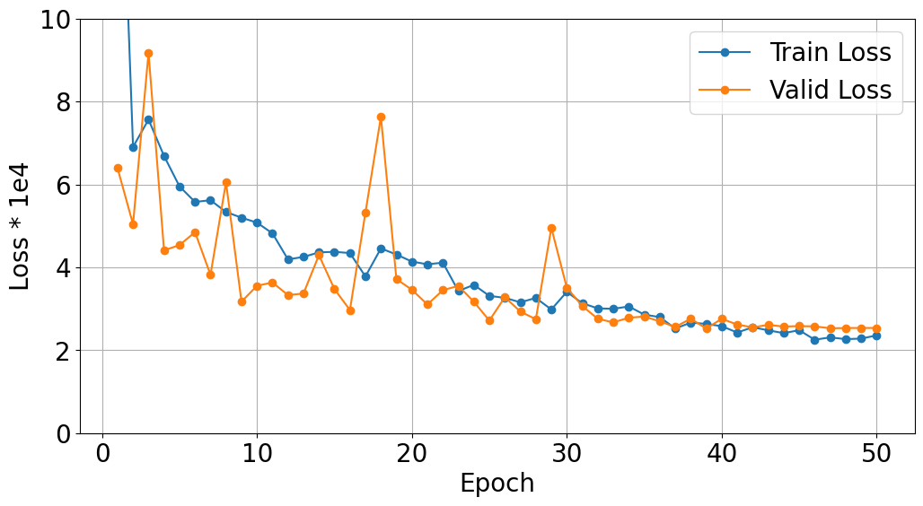
You can see the process of training accuracy surrogate function on Figure 11 and simularity surrogate function on Figure 11