Automated discovery of high-probability heralded schemes for path-entangled states

Marcello Armezzani marcello.armezzani@uni-tuebingen.de Machine Learning in Science Cluster, Department of Computer Science, Faculty of Science, University of Tübingen, Germany Colin P. Lualdi clualdi2@illinois.edu Materials Research Laboratory, The Grainger College of Engineering, University of Illinois Urbana-Champaign, Urbana, IL, USA Illinois Quantum Information Science and Technology Center, The Grainger College of Engineering, University of Illinois Urbana-Champaign, Urbana, IL, USA Department of Physics, The Grainger College of Engineering, University of Illinois Urbana-Champaign, Urbana, IL, USA Xuemei Gu xuemei.gu@uni-jena.de Institut für Festkörpertheorie und Optik, Friedrich-Schiller-Universität Jena, Jena, Germany Paul G. Kwiat kwiat@illinois.edu Materials Research Laboratory, The Grainger College of Engineering, University of Illinois Urbana-Champaign, Urbana, IL, USA Illinois Quantum Information Science and Technology Center, The Grainger College of Engineering, University of Illinois Urbana-Champaign, Urbana, IL, USA Department of Physics, The Grainger College of Engineering, University of Illinois Urbana-Champaign, Urbana, IL, USA Mario Krenn mario.krenn@uni-tuebingen.de Machine Learning in Science Cluster, Department of Computer Science, Faculty of Science, University of Tübingen, Germany

(July 28, 2026)

Abstract

Entangled states of light lie at the heart of photonic quantum technologies, from distributed quantum communication to quantum-enhanced measurement and information processing. Their practical generation, however, remains constrained by the weak interactions between photons, which make the deterministic assembly of large multiphoton entangled states a central challenge in quantum optics. In this work, we use AI techniques to discover heralded linear-optical schemes for path-entangled states and show that the resulting solutions can be elevated from individual circuits to a new scalable family. This family contains previously known constructions as special cases while generally providing exponential and super-exponential improvements over those, and its extension to broader classes of target states shows how automated discovery can reveal transferable physical understanding. By presenting compact experimental proposals for large path-entangled states, our results provide both a theoretical advance in photonic heralding and a route towards a substantial leap in experimentally accessible multiphoton entanglement.

Introduction— Entangled states of light are central resources for quantum technologies, with applications ranging from quantum communication and computation to sensing and tests of fundamental physics [44, 42, 19, 11, 10]. However, the generation of such states remains fundamentally constrained: in the absence of strong deterministic photon-photon interactions, linear optics alone generally cannot produce arbitrary multiphoton entanglement on demand [2, 41]. As a result, many critical photonic resources are generated probabilistically, either by post-selection or by heralding. The latter is especially important because it certifies the successful preparation of a desired state without consuming the state itself. Instead, auxiliary photons are measured in ancillary modes, and specific detection patterns announce the presence of the target state in the remaining modes. Combined with switchable quantum memories, this would enable periodic or on-demand preparation of the desired states, making heralded generation a natural route toward scalable photonic quantum technologies [21].

Among the paradigmatic examples of multiphoton entanglement are path-entangled states. In their simplest and most widely studied form, two-mode NOON states are defined as

\ket{\mathrm{NOON}_{N}}=\frac{\ket{N,0}+e^{i\phi}\ket{0,N}}{\sqrt{2}},

(1)

where $N$ is the total photon number and $\phi$ is an arbitrary relative phase between the two terms. These states have played a prominent role in quantum metrology, imaging, and lithography because of their enhanced phase sensitivity in the absence of loss [15, 22, 43]. They also represent a fundamental and peculiar form of entanglement alongside Bell and GHZ states [21].

A substantial body of work has established foundational heralding strategies for NOON states and related resources, including symmetric multiport constructions, vacuum- or photodetection-assisted schemes, and feed-forward-based approaches [60, 32, 45, 5, 38]. However, the landscape rapidly becomes more intricate as the target photon number increases, and the challenge is no longer just to parameterize a universal interferometer, but to identify input structures and heralding mechanisms that support exact cancellation of unwanted amplitudes with high success probability.

This challenge naturally suggests automated discovery. There is growing evidence that algorithmic design can uncover genuinely new quantum experiments rather than merely reproducing known intuition [35, 33, 1, 25, 20, 34]. Beside providing clear improvements in the efficiency and fidelity of state generation, the main conceptual question is whether such automated searches can be turned into physical understanding [36]: do they reveal new mechanisms, new general families, and new scaling laws?

In this work we answer this question affirmatively. Using a large-scale, fast automated search framework we discover a new, exact, and scalable family of circuits for generating states of the form shown in Eq. (1). This family reduces to known schemes for specific choices of parameters, but generally offers exponential and super-exponential enhancements in the success probability. This family also proves effective for the generation of multi-mode $\mathrm{NOON}$ states, improving over the best linear optical families [58]. We also report the discovery of improved solutions that are not part of the new family, and extend the same automated strategy to the so-called $m,m^{\prime}$ path-entangled states [28], obtaining passive linear-optical schemes that outperform the previously known nonlinear family for the same targets [23]. Finally, we address the experimental feasibility of our new solutions and propose future developments.

Automated discovery of a modular comb family— We build a universal multiport interferometer [47, 8] in a fast JAX [4] simulator, which we then optimize via stochastic gradient descent methods. We choose an input product state and an output target state; the latter exits in undetected modes while photon-number-resolving (PNR) detectors monitor the remaining (heralding) modes. From each simulated experiment we extract a heralding probability $p_{\mathrm{succ}}$ and a fidelity $F$ with respect to the target state, and we update the circuit to maximize both. Details are provided in Supplemental Material S.1 Optimization procedure.

Searching over many input and target states, and carefully analyzing the multitude of results produced, a particularly interesting general family emerges. Its first newly discovered member is the heralded circuit for $\mathrm{NOON}_{9}$ , shown in Fig. 1.

Refer to caption — Figure 1: Compact $\mathrm{NOON}_{9}$ heralded circuit obtained from the input $\ket{3,3,3,1,1}$ , which is the optimal choice within the new modular comb family. $\mathcal{F}_{3}$ is the Fourier multiport transformation acting on the bunched input photons and $B(\theta,\phi)$ is the beam splitter. See Supplemental Material S.2.3 $\mathrm{NOON}_{9}$ example for details.

For this specific case, the success probability increases by almost $1440\%$ with respect to the best existing scheme [45]. As additional benefits, the circuit requires fewer detectors and no longer relies solely on vacuum heralding—heralding on a detector not firing—which is known to be an unreliable experimental condition [40].

The general mechanism of the family can be described starting from

N=\sum_{\ell=1}^{L}r_{\ell}m_{\ell},

(2)

where $r_{\ell}\geq 2$ and $m_{\ell}\geq 1$ . The first part of the scheme takes an input state composed of $L$ packets $\bigotimes_{\ell=1}^{L}\ket{m_{\ell}}^{\otimes r_{\ell}}$ and propagates it through a multiport that leaves the two target modes populated by the modular comb

\ket{N-q,q},\quad q\in Q,

where $Q$ denotes the actual non-zero photon-number support of the comb. All the unwanted middle terms between $\ket{N,0}$ and $\ket{0,N}$ can be discarded through single-photon Fock filters, using a state $\ket{1,1}^{\otimes|B|}$ , where $B=\left\{\min(q,N-q):q\in Q,\ q\neq 0,N\right\}$ is the set of distinct symmetric filters. One mixes the target mode with an ancillary single photon on a beam splitter, and then keeps only the events in which one photon is detected again in the ancillary output. The heralded output is exactly the desired $\mathrm{NOON}$ state in Eq. (1) with a success probability of

p_{\mathrm{succ}}=2\frac{N!}{N^{N}}\prod_{\ell=1}^{L}\left(\frac{m_{\ell}^{m_{\ell}}}{m_{\ell}!}\right)^{r_{\ell}}\prod_{b\in B}\left(\frac{b}{b+1}\right)^{N}\left(\frac{N-b}{b+1}\right)^{2}.

(3)

Details on the derivation can be found in S.2.1 Explicit derivation. A remarkable aspect of Eq. (3) is that it contains, as limiting cases, the two main passive linear-optical families known before this work. Setting $L=1$ gives $N=rm$ . Choosing $r=N$ , $m=1$ produces no interior sectors to filter, and reduces the construction to the Pryde and White (PW) multiport family [45]. For even $N$ , choosing $r=2$ , $m=N/2$ gives the even- $N$ family of Zou, Pahlke, and Mathis (ZPM) [60]. These two limiting cases represent the previous state of the art for passive linear-optical $\mathrm{NOON}$ -state generation [21].

Furthermore, the nontrivial branches of the modular-comb family improve asymptotically over both of these known schemes. In Supplemental Material S.2.2 Asymptotic ratios, we show that explicit fixed-shape branches already satisfy

\frac{p_{\mathrm{succ}}}{p_{\rm PW}}\geq 10^{c_{\rm PW}N+O(1)},\frac{p_{\mathrm{succ}}}{p_{\rm ZPM}}\geq 10^{\frac{N}{2}\log_{10}N+O(N)},

(4)

where $c_{\rm PW}>0$ . Thus, the improvement is at least exponential with respect to PW and super-exponential with respect to ZPM. The exact optimized envelope is not monotonic because the best integer decomposition of $N$ and the optimal filter set depends on the value of $N$ . In Fig. 2, we show the exact optimized ratios together with finite- $N$ fits of the forms implied by Eq. (4).

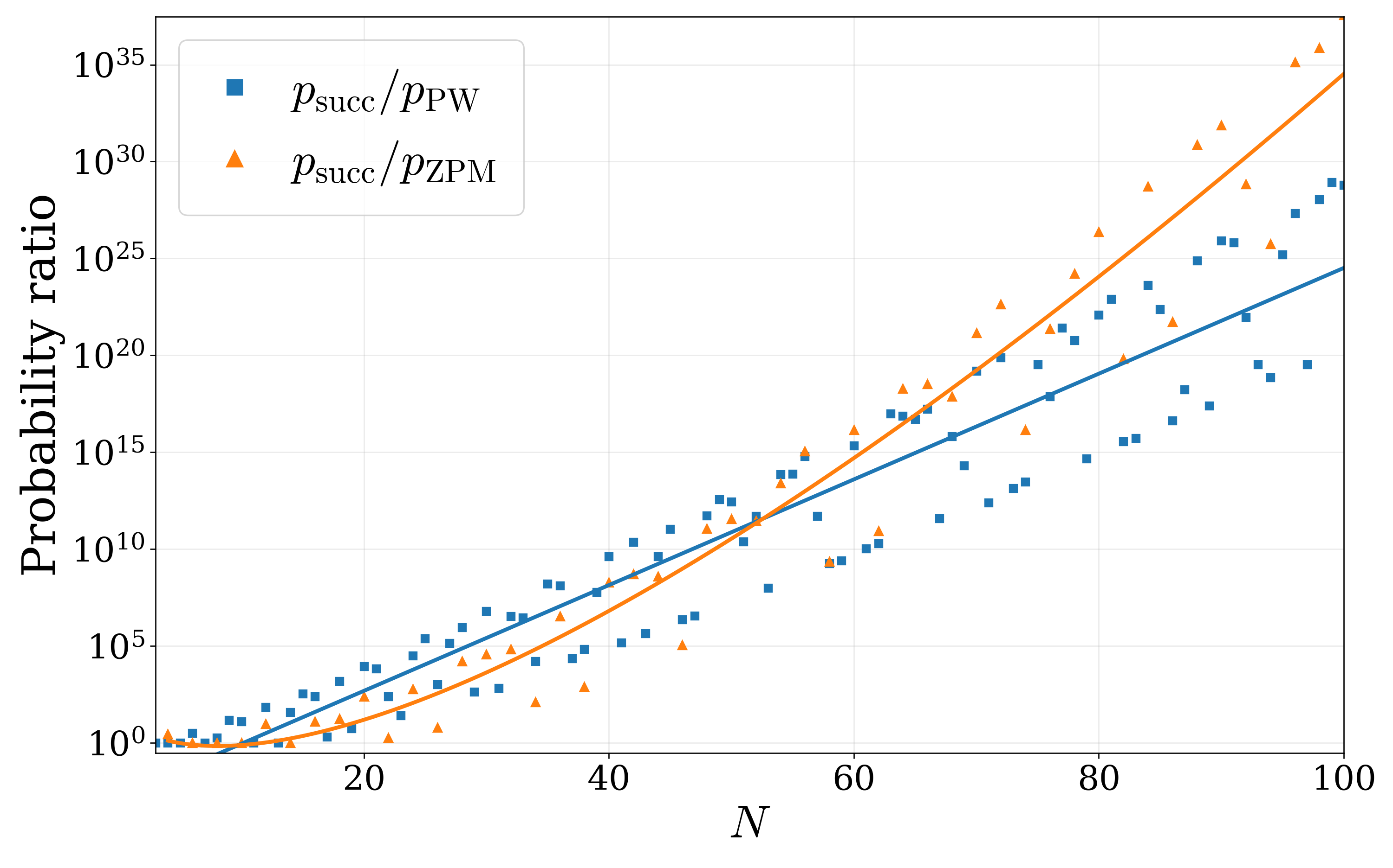
Understanding by generalization to the multi-mode $\mathrm{NOON}$ case— Scientific understanding is often revealed by the ability to generalize a mechanism beyond the particular case in which it was first identified [13]. We therefore test whether the modular-comb idea that emerged from the automated discovery for two-mode $\mathrm{NOON}$ states can be extended to multi-mode $\mathrm{NOON}$ states, which are particularly interesting for the simultaneous estimation of multiple parameters [27, 57]. We consider $N$ written as in Eq. (2), with the requirement $r_{\ell}\geq d$ , where $d$ is the number of modes of the target multi-mode $\mathrm{NOON}$ state. As before, we send $L$ packets through a multiport, which this time populates the modular comb (details in Supplemental Material S.3.1 Exact derivation)

\ket{N-|\mathbf{q}|,q_{1},\ldots,q_{d-1}},\qquad|\mathbf{q}|=\sum_{\mu=1}^{d-1}q_{\mu}.

Once again the single-photon Fock filters cancel out all the unwanted terms, leaving us with $\ket{N,0,\ldots,0},\ket{0,N,\ldots,0},\ldots,\ket{0,\ldots,N,0},\ket{0,\ldots,0,N}.$ This family improves over the best-performing linear-optical scheme presented by Zhang and Chan in [58]. In Supplemental Material S.3.2 Asymptotic ratio, we show that, for fixed $d$ , every fixed-shape branch of the modular-comb family satisfies

\frac{p_{\mathrm{succ}}^{(d)}}{p_{\rm ZC}^{(d)}}\geq N^{1/2}10^{c_{\rm ZC}^{(d)}N+O(1)},\qquad c_{\rm ZC}^{(d)}>0.

(5)

Here, $c_{\rm ZC}^{(d)}$ depends on the chosen fixed-shape branch. In Fig. 3, we plot the exact optimized ratios under the common universal filtering prescription. together with finite- $N$ fits to the regular-branch form $N^{1/2}10^{a_{d}N+b_{d}}$ .

Additional schemes— While the modular-comb family significantly improves on the previous state of the art, the new scheme is not necessarily optimal for all values of $N$ . Indeed, the automated discovery process reveals other superior solutions for specific target states that cannot be forced inside the same picture. In addition, to illustrate the flexibility of our approach, we also automate the discovery of the so-called $m,m^{\prime}$ states [28]

\frac{\ket{m,m^{\prime}}+\ket{m^{\prime},m}}{\sqrt{2}},

originally introduced to make $\mathrm{NOON}$ states more robust to loss. It is known in fact that advantages offered by $\mathrm{NOON}$ states rapidly decrease when loss is not negligible [49]. We summarize few examples of our findings in Table 1. These examples, while not exhaustive, serve as evidence that it is certainly possible to discover improved solutions that do not belong to general families; this was also recently shown in [50] for the three-mode, two-photon $\mathrm{NOON}$ state: $\left(\ket{2,0,0}+e^{i\alpha_{1}}\ket{0,2,0}+e^{i\alpha_{2}}\ket{0,0,2}\right)/\sqrt{3}$ .

Table 1: Examples of other discovered schemes that are not part of the newly discovered modular comb family. Automated discovery unlocks solutions that, beside achieving better success probabilities, reduce the required number of heralding modes (i.e., detectors) and eliminate complete vacuum conditions at the detectors. The explicit circuit of the new

\mathrm{NOON}_{8}

solution is shown in Fig. 4. The other schemes are explicitly shown in Supplemental Material S.4 Additional schemes.

Target state

Best known probability

New probability

Gain

Detectors condition

Source requirement

\displaystyle\frac{|5,0\rangle+|0,5\rangle}{\sqrt{2}}

\sim 7.68\%

[45]

\sim 9.17\%

\sim 19\%

old:

\ket{000}

new:

\ket{10}

old:

|1\rangle

new:

|2\rangle

\displaystyle\frac{|7,0\rangle+|0,7\rangle}{\sqrt{2}}

\sim 1.22\%

[45]

\sim 3.13\%

\sim 155\%

old:

\ket{00000}

new:

\ket{100}

old:

|1\rangle

new:

|2\rangle

\displaystyle\frac{|8,0\rangle-|0,8\rangle}{\sqrt{2}}

\sim 0.92\%

[60]

\sim 5.44\%

\sim 494\%

old:

\ket{1111}

new:

\ket{11}

old:

|4\rangle

new:

|3\rangle

\displaystyle\frac{|300\rangle+|030\rangle+|003\rangle}{\sqrt{3}}

\sim 0.69\%

[58]

\sim 4.17\%

comb family

\sim 14.71\%

\sim 2018\%

over old

\sim 253\%

over comb

old/comb:

\ket{111}

new:

\ket{10}

old:

|3\rangle

new/comb:

|1\rangle

\displaystyle\frac{|L,L-2\rangle+|L-2,L\rangle}{\sqrt{2}}

\scriptstyle\frac{8(L-1)}{L^{3}}\left(\frac{L-2}{L}\right)^{2L-4}

[23]

\scriptstyle\frac{1}{2}\left(1-\frac{1}{L}\right)^{2L-3}

quadratic

asymptotic gain

old:

\ket{L-2,L-2}

new:

\ket{11}

old: increasing

nonlinearities

new:

|L-1\rangle

Experimental feasibility— We now address the main experimental challenges that our proposed schemes would face. To do so, we analyze as examples the $\mathrm{NOON}_{9}$ and $\mathrm{NOON}_{8}$ circuits (Figs. 1 and 4, respectively). We first consider the consequences of inefficient heralding detectors. To model a detector with efficiency $\eta$ , we incorporate a beam splitter with transmissivity $\eta$ and reflectivity $1-\eta$ . The results are shown in Fig. 5, where we compare the new $\mathrm{NOON}_{9}$ and $\mathrm{NOON}_{8}$ circuits with the original PW and ZPM proposals, respectively. In the case of the new $\mathrm{NOON}_{9}$ scheme, both the fidelity and the heralding probability consistently exceed those of PW as the detector efficiency decreases. The fidelity also decreases more slowly with the new scheme. These results are due to the replacement of the full vacuum heralding condition $\ket{0000000}$ with the more reliable $\ket{110}$ . For $\mathrm{NOON}_{8}$ , we observe that the stricter ZPM $\ket{1111}$ heralding condition—compared to $\ket{11}$ for our new scheme (see Table 1)—better preserves the fidelity under decreasing efficiency, albeit at the cost of a greatly reduced heralding probability.

Experimental implementation of reliable heralding benefits from many options for efficient detectors, ranging from transition-edge sensors (e.g., [39, 16]) to superconducting nanowire single-photon detectors (e.g., [12, 51]), with various experimental trade-offs involving efficiency, photon-number-resolving capabilities, detection rate, and implementation complexity. Given the availability of detectors with up to at least 98% efficiency [48, 46], some with excellent photon-number resolution, we conclude that achieving high fidelity and heralding probability is possible.

Concerning the input states, both of the new schemes require $\ket{1}$ and $\ket{3}$ . Since the complexity of producing a Fock state generally increases with its size, our $\mathrm{NOON}_{8}$ result is advantageous compared to the original ZPM proposal, which requires $\ket{4}$ instead of $\ket{3}$ . Interestingly, the same does not apply to our $\mathrm{NOON}_{9}$ result: the original PW scheme requires only $\ket{1}$ states.

There has been significant progress in recent years with regard to generating these input states. For example, state-of-the-art single-photon sources can currently achieve success probabilities around 70% [29, 14]. While the efficient generation of larger Fock states such as $\ket{3}$ has yet to be demonstrated, multiple theoretical studies show that a “repeated addition” scheme can realize success probabilities in the tens of percent range with optimistic but realistic experimental parameters [38, 24]. Although realizing such devices remains a work in progress [18], such a protocol is far more promising than established methods based on single-pass spontaneous parametric down-conversion sources (e.g., [55, 9, 18]), which offer success probabilities that are lower by orders of magnitude. We also note that generating multiphoton states with a quantum-dot source is an emerging option [56, 30].

Finally, the small number of modes (and beamsplitters – five for each scheme) makes circuit construction straightforward. Loss can be minimized by leveraging free-space bulk optics: commercially available beamsplitters can offer $<$ 1% loss [52] and 97% coupling efficiency into single-mode fiber has been reported in the literature [59]. Even on-chip implementation may be possible given recent advances in low-loss SiN waveguide components featuring $\sim$ 0.01% splitter loss and up to $\sim$ 99% chip-to-fiber coupling [46]. Altogether, the experimental feasibility of efficient detectors, sources, and circuits lead us to believe that high-rate generation of $\mathrm{NOON}_{8}$ and $\mathrm{NOON}_{9}$ states based on our newly discovered schemes is attainable in the near future.

Outlook— In this work we presented a new exact family for the heralding of $\mathrm{NOON}$ states that improves exponentially and super-exponentially over existing schemes as $N$ grows. Additionally, we proved that the same family can be extended to multi-mode $\mathrm{NOON}$ states, and presented examples of superior schemes that do not belong to the new family.

Experimental implementations – We discussed experimental advantages offered by the newly discovered $\mathrm{NOON}_{8}$ and $\mathrm{NOON}_{9}$ circuits compared to existing schemes: the former requires smaller Fock states as inputs and the latter offers more favorable fidelity scaling under decreasing detector efficiency by virtue of minimizing vacuum heralding. These findings make these circuits strong candidates for near-future implementation.

Towards higher-photon-number heralding – Notable heralded-entanglement experiments [54, 3, 37, 26, 7, 6] have reported a maximum target-state size of four photons. Experimental implementation of our proposed circuits would therefore represent a significant advance. Looking at the whole batch of improved solutions we proposed, we notice how they are often associated with an input state which requires bunched photons. Realizing multiphoton Fock sources that are more efficient than the current state of the art is therefore another natural objective that will be hopefully pursued by the experimental community.

Scientific understanding through AI – The ideas discussed here are the result of an automated approach. We showed that automated search can be used not only to optimize heralded photonic circuits, but also to uncover simple physical principles behind high-probability state generation, therefore extracting pure scientific understanding that is by all means computer-inspired. Looking ahead, we deem crucial the progressive implementation of AI systems that are not only capable of producing improved results, but also of generalizing them to different scenarios, thereby becoming agents of understanding [36].

Increased search spaces – Advances in AI systems capable of generating scientific understanding must be accompanied by equally reliable and expressive physical simulators, since these simulators define the experimental reality on which automated scientific discovery relies. With respect to this work, it would be interesting to expand the search space by introducing conditional operations (based on mid-circuit measurements) and active non-linear elements [38, 17], and to model experimental imperfections directly into the optimization, instead of simply analyzing their effects on optimized solutions. Finally, it would be noteworthy to simulate and optimize complete experimental quantum tasks, instead of limiting ourselves to the heralding of the required resource states; such a wider approach could have the potential to completely change our perspective and produce unexpected and surprising ideas.

Acknowledgments— M.K. and M.A. acknowledge support by the European Research Council (ERC) under the European Union’s Horizon Europe research and innovation programme (ERC-2024-STG, 101165179, ArtDisQ) and from the German Research Foundation DFG (EXC 2064/1, Project 390727645). X.G. acknowledges support from the Alexander von Humboldt Foundation and the Deutsche Forschungsgemeinschaft (DFG, German Research Foundation) – Project-ID 398816777 – SFB 1375. P.G.K. and C.P.L. acknowledge that this material is based upon work supported by the National Science Foundation under Award No. 25-15092 and by the National Aeronautics and Space Administration under STTR Contract No. 80NSSC25CA031.

References

[1] S. Arlt, M. Krenn, and X. Gu (2026) Automated discovery of nonlocal photonic gates. Physical Review Research 8, pp. L022031. External Links: Document Cited by: Automated discovery of high-probability heralded schemes for path-entangled states.
[2] A. Aspuru-Guzik and P. Walther (2012) Photonic quantum simulators. Nature Physics 8 (4), pp. 285–291. External Links: Document Cited by: Automated discovery of high-probability heralded schemes for path-entangled states.
[3] S. Barz, G. Cronenberg, A. Zeilinger, and P. Walther (2010) Heralded generation of entangled photon pairs. Nature Photonics 4 (8), pp. 553–556. External Links: Document Cited by: Automated discovery of high-probability heralded schemes for path-entangled states.
[4] J. Bradbury, R. Frostig, P. Hawkins, M. J. Johnson, C. Leary, D. Maclaurin, S. Wanderman-Milne, and Q. Zhang (2018) JAX: composable transformations of Python+NumPy programs. Note: https://github.com/jax-ml/jax Cited by: Automated discovery of high-probability heralded schemes for path-entangled states.
[5] H. Cable and J. P. Dowling (2007) Efficient generation of large number-path entanglement using only linear optics and feed-forward. Physical Review Letters 99, pp. 163604. External Links: Document Cited by: Automated discovery of high-probability heralded schemes for path-entangled states.
[6] H. Cao, L. Hansen, F. Giorgino, L. Carosini, P. Zah’alka, F. Zilk, J. Loredo, and P. Walther (2024) Photonic source of heralded greenberger-horne-zeilinger states. Physical Review Letters 132 (13), pp. 130604. External Links: Document Cited by: Automated discovery of high-probability heralded schemes for path-entangled states.
[7] S. Chen, L. Peng, Y. Guo, X. Gu, X. Ding, R. Liu, J. Zhao, X. You, J. Qin, Y. Wang, et al. (2024) Heralded three-photon entanglement from a single-photon source on a photonic chip. Physical Review Letters 132 (13), pp. 130603. External Links: Document Cited by: Automated discovery of high-probability heralded schemes for path-entangled states.
[8] W. R. Clements, P. C. Humphreys, B. J. Metcalf, W. S. Kolthammer, and I. A. Walmsley (2016) Optimal design for universal multiport interferometers. Optica 3 (12), pp. 1460–1465. External Links: Document Cited by: Automated discovery of high-probability heralded schemes for path-entangled states.
[9] M. Cooper, L. J. Wright, C. Söller, and B. J. Smith (2013) Experimental generation of multi-photon Fock states. Optics Express 21 (5), pp. 5309–5317. External Links: Document Cited by: Automated discovery of high-probability heralded schemes for path-entangled states.
[10] C. Couteau, S. Barz, T. Durt, T. Gerrits, J. Huwer, R. Prevedel, J. Rarity, A. Shields, and G. Weihs (2023) Applications of single photons in quantum metrology, biology and the foundations of quantum physics. Nature Reviews Physics 5, pp. 354–363. External Links: Document Cited by: Automated discovery of high-probability heralded schemes for path-entangled states.
[11] C. Couteau, S. Barz, T. Durt, T. Gerrits, J. Huwer, R. Prevedel, J. Rarity, A. Shields, and G. Weihs (2023) Applications of single photons to quantum communication and computing. Nature Reviews Physics 5, pp. 326–338. External Links: Document Cited by: Automated discovery of high-probability heralded schemes for path-entangled states.
[12] S. I. Davis, A. Mueller, R. Valivarthi, N. Lauk, L. Narvaez, B. Korzh, A. D. Beyer, O. Cerri, M. Colangelo, K. K. Berggren, M. D. Shaw, S. Xie, N. Sinclair, and M. Spiropulu (2022-12) Improved heralded single-photon source with a photon-number-resolving superconducting nanowire detector. Physical Review Applied 18, pp. 064007. External Links: Document, Link Cited by: Automated discovery of high-probability heralded schemes for path-entangled states.
[13] H. W. de Regt (2017) Understanding scientific understanding. Oxford University Press, Oxford. External Links: ISBN 9780190652913, Link Cited by: Automated discovery of high-probability heralded schemes for path-entangled states.
[14] X. Ding, Y. Guo, M. Xu, R. Liu, G. Zou, J. Zhao, Z. Ge, Q. Zhang, H. Liu, L. Wang, M. Chen, H. Wang, Y. He, Y. Huo, C. Lu, and J. Pan (2025) High-efficiency single-photon source above the loss-tolerant threshold for efficient linear optical quantum computing. Nature Photonics 19 (4), pp. 387–391. External Links: Document Cited by: Automated discovery of high-probability heralded schemes for path-entangled states.
[15] J. P. Dowling (2008) Quantum optical metrology—the lowdown on high-N00N states. Contemporary Physics 49 (2), pp. 125–143. External Links: Document Cited by: Automated discovery of high-probability heralded schemes for path-entangled states.
[16] M. Eaton, A. Hossameldin, R. J. Birrittella, P. M. Alsing, C. C. Gerry, H. Dong, C. Cuevas, and O. Pfister (2023-01) Resolution of 100 photons and quantum generation of unbiased random numbers. Nature Photonics 17 (1), pp. 106–111. External Links: ISSN 1749-4893, Link, Document Cited by: Automated discovery of high-probability heralded schemes for path-entangled states.
[17] M. Engelkemeier, L. Lorz, S. De, B. Brecht, I. Dhand, M. B. Plenio, C. Silberhorn, and J. Sperling (2020-08) Quantum photonics with active feedback loops. Physical Review A 102, pp. 023712. External Links: Document, Link Cited by: Automated discovery of high-probability heralded schemes for path-entangled states.
[18] M. Engelkemeier, J. Sperling, J. Tiedau, S. Barkhofen, I. Dhand, M. B. Plenio, B. Brecht, and C. Silberhorn (2021) Climbing the fock ladder: advancing multiphoton state generation. External Links: 2105.03720, Link Cited by: Automated discovery of high-probability heralded schemes for path-entangled states.
[19] F. Flamini, N. Spagnolo, and F. Sciarrino (2019) Photonic quantum information processing: a review. Reports on Progress in Physics 82 (1), pp. 016001. External Links: Document Cited by: Automated discovery of high-probability heralded schemes for path-entangled states.
[20] S. A. Fldzhyan, M. Yu. Saygin, and S. P. Kulik (2021) Compact linear optical scheme for Bell state generation. Physical Review Research 3, pp. 043031. External Links: Document Cited by: Automated discovery of high-probability heralded schemes for path-entangled states.
[21] I. Forbes, F. Ghafari, E. C. R. Deacon, S. P. Singh, E. Lavie, P. Yard, R. D. Shaw, A. Laing, and N. Tischler (2025) Heralded generation of entanglement with photons. Reports on Progress in Physics 88 (8), pp. 086002. External Links: Document Cited by: Automated discovery of high-probability heralded schemes for path-entangled states, Automated discovery of high-probability heralded schemes for path-entangled states, Automated discovery of high-probability heralded schemes for path-entangled states.
[22] V. Giovannetti, S. Lloyd, and L. Maccone (2011) Advances in quantum metrology. Nature Photonics 5 (4), pp. 222–229. External Links: Document Cited by: Automated discovery of high-probability heralded schemes for path-entangled states.
[23] R. T. Glasser, H. Cable, J. P. Dowling, F. De Martini, F. Sciarrino, and C. Vitelli (2008) Entanglement-seeded-dual optical parametric amplification: applications to quantum communication, imaging, and metrology. Physical Review A 78, pp. 012339. External Links: Document Cited by: Table 1, Automated discovery of high-probability heralded schemes for path-entangled states.
[24] B. L. Glebov, J. Fan, and A. Migdall (2014) Photon number squeezing in repeated parametric downconversion with ancillary photon-number measurements. Optics Express 22 (17), pp. 20358–20365. External Links: Document Cited by: Automated discovery of high-probability heralded schemes for path-entangled states.
[25] F. V. Gubarev, I. V. Dyakonov, M. Yu. Saygin, G. I. Struchalin, S. S. Straupe, and S. P. Kulik (2020) Improved heralded schemes to generate entangled states from single photons. Physical Review A 102, pp. 012604. External Links: Document Cited by: Automated discovery of high-probability heralded schemes for path-entangled states.
[26] D. R. Hamel, L. K. Shalm, H. Hübel, A. J. Miller, F. Marsili, V. B. Verma, R. P. Mirin, S. W. Nam, K. J. Resch, and T. Jennewein (2014) Direct generation of three-photon polarization entanglement. Nature Photonics 8 (10), pp. 801–807. External Links: Document Cited by: Automated discovery of high-probability heralded schemes for path-entangled states.
[27] P. C. Humphreys, M. Barbieri, A. Datta, and I. A. Walmsley (2013) Quantum enhanced multiple phase estimation. Physical Review Letters 111, pp. 070403. External Links: Document Cited by: Automated discovery of high-probability heralded schemes for path-entangled states.
[28] S. D. Huver, C. F. Wildfeuer, and J. P. Dowling (2008) Entangled Fock states for robust quantum optical metrology, imaging, and sensing. Physical Review A 78, pp. 063828. External Links: Document Cited by: Automated discovery of high-probability heralded schemes for path-entangled states, Automated discovery of high-probability heralded schemes for path-entangled states.
[29] F. Kaneda and P. G. Kwiat (2019) High-efficiency single-photon generation via large-scale active time multiplexing. Science Advances 5 (10), pp. eaaw8586. External Links: Document Cited by: Automated discovery of high-probability heralded schemes for path-entangled states.
[30] Y. Karli, I. Avila Arenas, C. Schimpf, A. J. Garcia Junior, S. Manna, F. Kappe, R. Schwarz, G. Undeutsch, M. Aigner, M. Peter, S. F. Covre da Silva, A. Rastelli, G. Weihs, and V. Remesh (2025-08) Passive demultiplexed two-photon state generation from a quantum dot. npj Quantum Information 11 (1), pp. 139. External Links: ISSN 2056-6387, Link, Document Cited by: Automated discovery of high-probability heralded schemes for path-entangled states.
[31] D. P. Kingma and J. Ba (2014) Adam: a method for stochastic optimization. arXiv preprint arXiv:1412.6980. External Links: Document Cited by: S.1 Optimization procedure.
[32] P. Kok, H. Lee, and J. P. Dowling (2002) Creation of large-photon-number path entanglement conditioned on photodetection. Physical Review A 65, pp. 052104. External Links: Document Cited by: Automated discovery of high-probability heralded schemes for path-entangled states.
[33] M. Krenn, M. Erhard, and A. Zeilinger (2020) Computer-inspired quantum experiments. Nature Reviews Physics 2 (11), pp. 649–661. External Links: Document Cited by: Automated discovery of high-probability heralded schemes for path-entangled states.
[34] M. Krenn, J. Landgraf, T. Foesel, and F. Marquardt (2023) Artificial intelligence and machine learning for quantum technologies. Physical Review A 107, pp. 010101. External Links: Document Cited by: Automated discovery of high-probability heralded schemes for path-entangled states.
[35] M. Krenn, M. Malik, R. Fickler, R. Lapkiewicz, and A. Zeilinger (2016) Automated search for new quantum experiments. Physical Review Letters 116, pp. 090405. External Links: Document Cited by: Automated discovery of high-probability heralded schemes for path-entangled states.
[36] M. Krenn, R. Pollice, S. Y. Guo, M. Aldeghi, A. Cervera-Lierta, P. Friederich, G. dos Passos Gomes, F. Häse, A. Jinich, A. Nigam, Z. Yao, and A. Aspuru-Guzik (2022) On scientific understanding with artificial intelligence. Nature Reviews Physics 4 (12), pp. 761–769. External Links: Document Cited by: Automated discovery of high-probability heralded schemes for path-entangled states, Automated discovery of high-probability heralded schemes for path-entangled states.
[37] J. C. Matthews, A. Politi, D. Bonneau, and J. L. O’Brien (2011) Heralding two-photon and four-photon path entanglement on a chip. Physical Review Letters 107 (16), pp. 163602. External Links: Document Cited by: Automated discovery of high-probability heralded schemes for path-entangled states.
[38] K. T. McCusker and P. G. Kwiat (2009) Efficient optical quantum state engineering. Physical Review Letters 103, pp. 163602. External Links: Document Cited by: Automated discovery of high-probability heralded schemes for path-entangled states, Automated discovery of high-probability heralded schemes for path-entangled states, Automated discovery of high-probability heralded schemes for path-entangled states.
[39] L. A. Morais, T. Weinhold, M. P. d. Almeida, J. Combes, M. Rambach, A. Lita, T. Gerrits, S. W. Nam, A. G. White, and G. Gillett (2024-05) Precisely determining photon-number in real time. Quantum 8, pp. 1355. External Links: Document, Link, ISSN 2521-327X Cited by: Automated discovery of high-probability heralded schemes for path-entangled states.
[40] C. M. Nunn, J. D. Franson, and T. B. Pittman (2021-09) Heralding on the detection of zero photons. Physical Review A 104, pp. 033717. External Links: Document, Link Cited by: Automated discovery of high-probability heralded schemes for path-entangled states.
[41] J. L. O’Brien, A. Furusawa, and J. Vučkovi’c (2009) Photonic quantum technologies. Nature Photonics 3 (12), pp. 687–695. External Links: Document Cited by: Automated discovery of high-probability heralded schemes for path-entangled states.
[42] J. Pan, Z. Chen, C. Lu, H. Weinfurter, A. Zeilinger, and M. Żukowski (2012) Multiphoton entanglement and interferometry. Reviews of Modern Physics 84 (2), pp. 777–838. External Links: Document Cited by: Automated discovery of high-probability heralded schemes for path-entangled states.
[43] L. Pezzè, A. Smerzi, M. K. Oberthaler, R. Schmied, and P. Treutlein (2018) Quantum metrology with nonclassical states of atomic ensembles. Reviews of Modern Physics 90, pp. 035005. External Links: Document Cited by: Automated discovery of high-probability heralded schemes for path-entangled states.
[44] R. Prevedel, M. Aspelmeyer, C. Brukner, A. Zeilinger, and T. D. Jennewein (2007-02) Photonic entanglement as a resource in quantum computation and quantum communication. Journal of the Optical Society of America B 24 (2), pp. 241–248. External Links: Document Cited by: Automated discovery of high-probability heralded schemes for path-entangled states.
[45] G. J. Pryde and A. G. White (2003) Creation of maximally entangled photon-number states using optical fiber multiports. Physical Review A 68, pp. 052315. External Links: Document Cited by: Table 1, Table 1, Automated discovery of high-probability heralded schemes for path-entangled states, Automated discovery of high-probability heralded schemes for path-entangled states, Automated discovery of high-probability heralded schemes for path-entangled states.
[46] PsiQuantum team (2025-05) A manufacturable platform for photonic quantum computing. Nature 641 (8064), pp. 876–883. External Links: ISSN 1476-4687, Link, Document Cited by: Automated discovery of high-probability heralded schemes for path-entangled states, Automated discovery of high-probability heralded schemes for path-entangled states.
[47] M. Reck, A. Zeilinger, H. J. Bernstein, and P. Bertani (1994) Experimental realization of any discrete unitary operator. Physical Review Letters 73, pp. 58–61. External Links: Document Cited by: Automated discovery of high-probability heralded schemes for path-entangled states.
[48] D. V. Reddy, R. R. Nerem, S. W. Nam, R. P. Mirin, and V. B. Verma (2020-12) Superconducting nanowire single-photon detectors with 98% system detection efficiency at 1550 nm. Optica 7 (12), pp. 1649–1653. External Links: Link, Document Cited by: Automated discovery of high-probability heralded schemes for path-entangled states.
[49] M. A. Rubin and S. Kaushik (2007) Loss-induced limits to phase measurement precision with maximally entangled states. Physical Review A 75, pp. 053805. External Links: Document Cited by: Automated discovery of high-probability heralded schemes for path-entangled states.
[50] S. P. Singh, E. Bazzazi, D. N. Bernal-García, S. White, H. J. Latief, A. Goldingay, S. Rogge, S. Slussarenko, F. Ghafari, E. Polino, and N. Tischler (2025) Heralded generation of a three-mode NOON state. arXiv preprint arXiv:2512.08458. External Links: 2512.08458 Cited by: Automated discovery of high-probability heralded schemes for path-entangled states.
[51] L. Stasi, T. Taher, G. V. Resta, H. Zbinden, R. Thew, and F. Bussières (2025-01) Enhanced Detection Rate and High Photon-Number Efficiencies with a Scalable Parallel SNSPD. ACS Photonics 12 (1), pp. 320–329. External Links: Link, Document Cited by: Automated discovery of high-probability heralded schemes for path-entangled states.
[52] Thorlabs (2026) UV Fused Silica Broadband Plate Beamsplitters (600–1700 nm). Note: Accessed 27 July 2026 Cited by: Automated discovery of high-probability heralded schemes for path-entangled states.
[53] N. M. VanMeter, P. Lougovski, D. B. Uskov, K. Kieling, J. Eisert, and J. P. Dowling (2007) General linear-optical quantum state generation scheme: applications to maximally path-entangled states. Physical Review A 76, pp. 063808. External Links: Document Cited by: S.4.1 Two- and three-mode $\mathrm{NOON}$ states.
[54] C. Wagenknecht, C. Li, A. Reingruber, X. Bao, A. Goebel, Y. Chen, Q. Zhang, K. Chen, and J. Pan (2010) Experimental demonstration of a heralded entanglement source. Nature Photonics 4 (8), pp. 549–552. External Links: Document Cited by: Automated discovery of high-probability heralded schemes for path-entangled states.
[55] E. Waks, E. Diamanti, and Y. Yamamoto (2006) Generation of photon number states. New Journal of Physics 8, pp. 4. External Links: Document Cited by: Automated discovery of high-probability heralded schemes for path-entangled states.
[56] B. Wu, L. Liu, H. Liu, X. Mao, X. Wang, H. Ni, Z. Niu, and Z. Yuan (2026-04) Purcell-enhanced two-photon emission from a quantum dot via dark-state biexciton loading. Nature Materials 25 (4), pp. 595–601. External Links: ISSN 1476-4660, Link, Document Cited by: Automated discovery of high-probability heralded schemes for path-entangled states.
[57] J. Yue, Y. Zhang, and H. Fan (2014) Quantum-enhanced metrology for multiple phase estimation with noise. Scientific Reports 4, pp. 5933. External Links: Document Cited by: Automated discovery of high-probability heralded schemes for path-entangled states.
[58] L. Zhang and K. W. C. Chan (2018) Scalable generation of multi-mode NOON states for quantum multiple-phase estimation. Scientific Reports 8, pp. 11440. External Links: Document Cited by: Table 1, S.3.2 Asymptotic ratio, Automated discovery of high-probability heralded schemes for path-entangled states, Automated discovery of high-probability heralded schemes for path-entangled states.
[59] H. Zhong, Y. Li, W. Li, L. Peng, Z. Su, Y. Hu, Y. He, X. Ding, W. Zhang, H. Li, L. Zhang, Z. Wang, L. You, X. Wang, X. Jiang, L. Li, Y. Chen, N. Liu, C. Lu, and J. Pan (2018-12) 12-photon entanglement and scalable scattershot boson sampling with optimal entangled-photon pairs from parametric down-conversion. Physical Review Letters 121, pp. 250505. External Links: Document, Link Cited by: Automated discovery of high-probability heralded schemes for path-entangled states.
[60] X. B. Zou, K. Pahlke, and W. Mathis (2002) Generation of entangled photon states by using linear optical elements. Physical Review A 66, pp. 014102. External Links: Document Cited by: Table 1, Automated discovery of high-probability heralded schemes for path-entangled states, Automated discovery of high-probability heralded schemes for path-entangled states.

Supplemental Material for:
Automated discovery of high-probability heralded schemes for path-entangled states

S.1 Optimization procedure

We consider an $M$ -mode passive linear-optical circuit decomposed into phase shifters and beam splitters. A phase shifter on mode $i$ acts as

P_{i}(\varphi)\ket{n_{i}}=e^{in_{i}\varphi}\ket{n_{i}}.

For a beam splitter acting on modes $i,j$ , we use the convention

\hat{a}_{i}^{\dagger}\longmapsto t\,\hat{a}_{i}^{\dagger}+r\,\hat{a}_{j}^{\dagger},\qquad\hat{a}_{j}^{\dagger}\longmapsto-r^{*}\,\hat{a}_{i}^{\dagger}+t\,\hat{a}_{j}^{\dagger},

where

t=\cos\theta,\qquad r=e^{i\phi}\sin\theta.

In the two-mode Fock basis, the same beam splitter is evaluated exactly as

B_{ij}(\theta,\phi)\ket{m,n}=\sum_{u=0}^{m+n}A_{m,n}^{(u)}(\theta,\phi)\ket{u,m+n-u},

with

A_{m,n}^{(u)}=\sqrt{\frac{u!\,(m+n-u)!}{m!\,n!}}\sum_{p=p_{\min}}^{p_{\max}}\binom{m}{p}\binom{n}{u-p}t^{n+2p-u}r^{m-p}(-r^{*})^{u-p},

where

p_{\min}=\max(0,u-n),\qquad p_{\max}=\min(m,u).

The full interferometer is obtained by composing these elementary maps according to a Reck or Clements mesh. In addition, the total photon number is conserved. Therefore, for a fixed input product Fock state

\ket{\mathbf{n}_{\mathrm{in}}}=\ket{n_{1},n_{2},\ldots,n_{M}},\qquad N=\sum_{i=1}^{M}n_{i},

the simulation is restricted to the fixed- $N$ Fock sector

\mathcal{H}_{N,M}=\mathrm{span}\left\{\ket{\mathbf{n}}:\sum_{i=1}^{M}n_{i}=N\right\}.

Let $\mathcal{T}$ denote the set of target modes and $\mathcal{D}$ the set of detected modes, with $\mathcal{T}\cap\mathcal{D}=\varnothing$ . The desired target state is written as

\ket{\psi_{\star}}=\sum_{\mathbf{a}}\alpha_{\mathbf{a}}\ket{\mathbf{a}}_{\mathcal{T}},\qquad\sum_{\mathbf{a}}|\alpha_{\mathbf{a}}|^{2}=1.

After the interferometer $U(\bm{\xi})$ , where $\bm{\xi}$ denotes all beam-splitter and phase-shifter parameters, the global output state is

\ket{\Psi(\bm{\xi})}=U(\bm{\xi})\ket{\mathbf{n}_{\mathrm{in}}}.

For a photon-number-resolving detector pattern $\mathbf{h}$ on the detected modes, we define the corresponding unnormalized conditional state on the target modes as

\ket{\psi_{\mathbf{h}}(\bm{\xi})}={}_{\mathcal{D}}\!\bra{\mathbf{h}}\Psi(\bm{\xi})\rangle.

Its heralding probability is

p_{\mathbf{h}}(\bm{\xi})=\norm{\ket{\psi_{\mathbf{h}}(\bm{\xi})}}^{2},

while its overlap with the desired target state is

q_{\mathbf{h}}(\bm{\xi})=\left|\innerproduct{\psi_{\star}}{\psi_{\mathbf{h}}(\bm{\xi})}\right|^{2}.

For a single accepted heralding pattern, the conditional fidelity would therefore be

F_{\mathbf{h}}(\bm{\xi})=\frac{q_{\mathbf{h}}(\bm{\xi})}{p_{\mathbf{h}}(\bm{\xi})}.

In the optimization, however, we do not choose a single heralding pattern in advance. Instead, we define a finite bank of possible detector outcomes,

\mathcal{H}=\{\mathbf{h}_{1},\mathbf{h}_{2},\ldots,\mathbf{h}_{W}\},

and assign to each pattern a trainable real logit $u_{\mathbf{h}}$ . The corresponding soft acceptance weight is

w_{\mathbf{h}}=\sigma(u_{\mathbf{h}})=\frac{1}{1+e^{-u_{\mathbf{h}}}}.

The total heralding probability used during training is then

p_{\mathrm{succ}}(\bm{\xi},\mathbf{u})=\sum_{\mathbf{h}\in\mathcal{H}}w_{\mathbf{h}}\,p_{\mathbf{h}}(\bm{\xi}),

and the corresponding fidelity is

F(\bm{\xi},\mathbf{u})=\frac{\sum_{\mathbf{h}\in\mathcal{H}}w_{\mathbf{h}}\,q_{\mathbf{h}}(\bm{\xi})}{p_{\mathrm{succ}}(\bm{\xi},\mathbf{u})}.

Thus the discrete problem of selecting an accepted set of detector outcomes is embedded into a continuous problem through the weights $w_{\mathbf{h}}$ .

The loss function used in the automated discovery is

\mathcal{L}(\bm{\xi},\mathbf{u})=1-F(\bm{\xi},\mathbf{u})+\lambda_{p}\frac{1}{p_{\mathrm{succ}}(\bm{\xi},\mathbf{u})},

(S.1.1)

with $\lambda_{p}>0$ . The first term enforces fidelity with the target state, while the second term penalizes solutions whose high fidelity is obtained only at vanishing heralding probability.

This construction converts the original mixed discrete–continuous search into a differentiable optimization problem. The beam-splitter angles, beam-splitter phases, phase-shifter phases, and heralding logits are all continuous trainable variables

\left\{\theta_{\ell},\phi_{\ell},\varphi_{\ell},u_{\mathbf{h}}\right\}.

This implementation is well suited to JAX because the computational graph is fixed once $M$ , the input photon number, the target modes, and the detector-pattern bank are specified. The Fock basis, beam-splitter transition tables, detector-pattern maps, and heralding groups are precomputed as static arrays, while only the optical parameters and heralding logits remain trainable. The forward pass is then expressed as a sequence of array operations over fixed-shape tensors: propagation through the interferometer, grouping of amplitudes by detector outcome, evaluation of $p_{\mathbf{h}}$ and $q_{\mathbf{h}}$ , and finally evaluation of Eq. (S.1.1). This allows the whole loss and its gradients to be compiled with XLA (Accelerated Linear Algebra) through JAX’s just-in-time compilation and executed efficiently on GPUs. Gradients with respect to all continuous variables are obtained by automatic differentiation, and the resulting objective is optimized with the Adam optimizer [31] from many random initializations.

S.2 Modular comb family

S.2.1 Explicit derivation

We explicitly derive the general modular-comb construction of the discovered family. The target photon number is written as

N=\sum_{\ell=1}^{L}r_{\ell}m_{\ell}.

The input consists of $L$ bunched packets and of the ancillary photons used by the Fock filters,

\ket{\psi_{\rm in}}=\bigotimes_{\ell=1}^{L}\ket{m_{\ell}}^{\otimes r_{\ell}}\otimes\ket{1,1}^{\otimes|B|}.

The first factor generates the modular comb on the two target modes, while each ancillary pair $\ket{1,1}$ implements one symmetric Fock filter on the two rails. The set $B$ of filters is defined below. We require $r_{\ell}\geq 2$ , so that each packet can coherently populate both target rails.

Let the input creation operators of the $\ell$ -th packet be

\hat{u}_{\ell,0}^{\dagger},\hat{u}_{\ell,1}^{\dagger},\ldots,\hat{u}_{\ell,r_{\ell}-1}^{\dagger},

and the output modes denoted by

\hat{o}_{\ell,0}^{\dagger},\hat{o}_{\ell,1}^{\dagger},\hat{h}_{\ell,2}^{\dagger},\ldots,\hat{h}_{\ell,r_{\ell}-1}^{\dagger},

where $\hat{o}_{\ell,0}^{\dagger}$ and $\hat{o}_{\ell,1}^{\dagger}$ are the two packet rails that will later be coherently collected into the target modes, while $\hat{h}_{\ell,k}^{\dagger}$ will be similarly collected into heralding modes. The multiport transformation is of Fourier type:

\hat{u}_{\ell,q}^{\dagger}\longrightarrow\frac{1}{\sqrt{r_{\ell}}}\left(\hat{o}_{\ell,0}^{\dagger}+\zeta_{r_{\ell}}^{q}\hat{o}_{\ell,1}^{\dagger}+\sum_{k=2}^{r_{\ell}-1}\zeta_{r_{\ell}}^{qk}\hat{h}_{\ell,k}^{\dagger}\right),\qquad\zeta_{r_{\ell}}=e^{2\pi i/r_{\ell}}.

The two packet rails are then combined, for each target rail separately, into the final target modes $\hat{a}_{0}^{\dagger}$ and $\hat{a}_{1}^{\dagger}$ . We choose real weights $\lambda_{\ell}\geq 0$ such that

\sum_{\ell=1}^{L}\lambda_{\ell}=1.

For $\mu=0,1$ , the collection unitary is chosen so that

\hat{o}_{\ell,\mu}^{\dagger}\longrightarrow\sqrt{\lambda_{\ell}}\,\hat{a}_{\mu}^{\dagger}+\sum_{s=1}^{L-1}w_{\mu,s\ell}\,\hat{g}_{\mu,s}^{\dagger}.

The modes $\hat{g}_{\mu,s}^{\dagger}$ are additional heralding modes. The coefficients $w_{\mu,s\ell}$ complete the normalized row

\left(\sqrt{\lambda_{1}},\sqrt{\lambda_{2}},\ldots,\sqrt{\lambda_{L}}\right)

to an $L$ -mode passive unitary. Combining the multiports and the collection unitaries, the full state before the vacuum heralding is

\ket{\Psi_{\rm pre}}=\prod_{\ell=1}^{L}\prod_{q=0}^{r_{\ell}-1}\frac{1}{\sqrt{m_{\ell}!}}\Bigg[\frac{1}{\sqrt{r_{\ell}}}\Bigg(\sqrt{\lambda_{\ell}}\,\hat{a}_{0}^{\dagger}+\sum_{s=1}^{L-1}w_{0,s\ell}\hat{g}_{0,s}^{\dagger}+\zeta_{r_{\ell}}^{q}\left(\sqrt{\lambda_{\ell}}\,\hat{a}_{1}^{\dagger}+\sum_{s=1}^{L-1}w_{1,s\ell}\hat{g}_{1,s}^{\dagger}\right)+\sum_{k=2}^{r_{\ell}-1}\zeta_{r_{\ell}}^{qk}\hat{h}_{\ell,k}^{\dagger}\Bigg)\Bigg]^{m_{\ell}}\ket{0}.

The vacuum heralding condition projects all modes

\hat{h}_{\ell,k}^{\dagger}\quad(k=2,\ldots,r_{\ell}-1),\qquad\hat{g}_{\mu,s}^{\dagger}\quad(\mu=0,1,\;s=1,\ldots,L-1)

onto vacuum. The resulting unnormalized two-mode state is therefore

\ket{\psi_{\rm tar}(\bm{\lambda})}=C(\bm{\lambda})\prod_{\ell=1}^{L}\prod_{q=0}^{r_{\ell}-1}\left(\hat{a}_{0}^{\dagger}+\zeta_{r_{\ell}}^{q}\hat{a}_{1}^{\dagger}\right)^{m_{\ell}}\ket{0},

with

C(\bm{\lambda})=\prod_{\ell=1}^{L}\frac{\left(\lambda_{\ell}/r_{\ell}\right)^{r_{\ell}m_{\ell}/2}}{\left(m_{\ell}!\right)^{r_{\ell}/2}}.

Using the identity

\prod_{q=0}^{r-1}\left(x+\zeta_{r}^{q}y\right)=x^{r}+(-1)^{r+1}y^{r},

we obtain

\ket{\psi_{\rm tar}(\bm{\lambda})}=C(\bm{\lambda})\prod_{\ell=1}^{L}\left[\left(\hat{a}_{0}^{\dagger}\right)^{r_{\ell}}+(-1)^{r_{\ell}+1}\left(\hat{a}_{1}^{\dagger}\right)^{r_{\ell}}\right]^{m_{\ell}}\ket{0}.

Expanding each packet, every term contributes to a two-mode sector of the form

\ket{N-q(\bm{j}),q(\bm{j})},\qquad q(\bm{j})=\sum_{\ell=1}^{L}r_{\ell}j_{\ell},\qquad j_{\ell}=0,\ldots,m_{\ell}.

The set of photon numbers that can arise before contributions to the same sector are coherently combined is

\widetilde{Q}=\left\{\sum_{\ell=1}^{L}r_{\ell}j_{\ell}:j_{\ell}=0,\ldots,m_{\ell}\right\}.

To determine the actual photon-number support, define the polynomial

P(z)=\prod_{\ell=1}^{L}\left[1+(-1)^{r_{\ell}+1}z^{r_{\ell}}\right]^{m_{\ell}}=\sum_{q=0}^{N}A_{q}z^{q}.

The conditional state can then be written as

\ket{\psi_{\rm tar}(\bm{\lambda})}=C(\bm{\lambda})\sum_{q=0}^{N}A_{q}\left(\hat{a}_{0}^{\dagger}\right)^{N-q}\left(\hat{a}_{1}^{\dagger}\right)^{q}\ket{0}.

The photon-number support is therefore the modular comb

Q=\left\{q\in\widetilde{Q}:A_{q}\neq 0\right\}.

Since

A_{0}=1,\qquad A_{N}=(-1)^{N+\sum_{\ell=1}^{L}m_{\ell}},

the two desired edge sectors $q=0$ and $q=N$ are always present. All other populated sectors are removed by single-photon Fock filters. Since the sectors $q$ and $N-q$ are removed by the same symmetric filter, the distinct filter set is

B=\left\{\min(q,N-q):q\in Q,\;q\neq 0,N\right\}.

Different tuples $\bm{j}$ may give the same value of $q$ . Their contributions are coherently combined in the coefficient $A_{q}$ and may cancel exactly. This does not affect the construction, because the filters act on photon-number sectors rather than on the individual paths that contribute to their amplitudes.

We now derive the action of one filter. Consider one target mode $\hat{a}_{\mu}^{\dagger}$ and one ancillary mode $\hat{c}^{\dagger}$ , mixed on a beam splitter with real amplitudes

t=\cos\theta,\qquad s=\sin\theta.

Using the convention we introduced in the previous section we get

\hat{a}_{\mu}^{\dagger}\longrightarrow t\hat{a}_{\mu}^{\dagger}+s\hat{c}^{\dagger},\qquad\hat{c}^{\dagger}\longrightarrow-s\hat{a}_{\mu}^{\dagger}+t\hat{c}^{\dagger}.

Starting from $k$ photons in the target mode and one photon in the ancillary mode, and heralding again on one photon in the ancillary output, the target component is multiplied by

f(k)=t^{k-1}\left(t^{2}-ks^{2}\right).

To remove a sector in which one rail contains $b$ photons, we choose

t_{b}^{2}=\frac{b}{b+1},\qquad s_{b}^{2}=\frac{1}{b+1},

then impose $f(b)=0$ . Applying the same filter to both rails removes both $\ket{N-b,b}$ and $\ket{b,N-b}$ .

On an edge component, the two target rails contain $N$ and $0$ photons. A filter tuned to $b$ therefore contributes the edge amplitude

f(N)f(0)=-t_{b}^{N}\frac{N-b}{b+1}.

Thus the edge survival probability of one symmetric filter is

\left|f(N)f(0)\right|^{2}=\left(\frac{b}{b+1}\right)^{N}\left(\frac{N-b}{b+1}\right)^{2}.

The unfiltered probability weight of the two edge sectors is

p_{\rm edge}(\bm{\lambda})=2N!\prod_{\ell=1}^{L}\frac{\left(\lambda_{\ell}/r_{\ell}\right)^{r_{\ell}m_{\ell}}}{\left(m_{\ell}!\right)^{r_{\ell}}}.

Maximizing this expression over $\lambda_{\ell}$ , under the constraint $\sum_{\ell}\lambda_{\ell}=1$ , gives

\lambda_{\ell}=\frac{r_{\ell}m_{\ell}}{N}.

With this choice,

p_{\rm edge}^{(L)}=2\frac{N!}{N^{N}}\prod_{\ell=1}^{L}\left(\frac{m_{\ell}^{m_{\ell}}}{m_{\ell}!}\right)^{r_{\ell}}.

Multiplying by the survival probability of every distinct filter $b\in B$ , we obtain

p_{\mathrm{succ}}^{(L)}=2\frac{N!}{N^{N}}\prod_{\ell=1}^{L}\left(\frac{m_{\ell}^{m_{\ell}}}{m_{\ell}!}\right)^{r_{\ell}}\prod_{b\in B}\left(\frac{b}{b+1}\right)^{N}\left(\frac{N-b}{b+1}\right)^{2}.

(S.2.1.1)

This is Eq. (3) in the main text.

S.2.2 Asymptotic ratios

We derive the asymptotic behavior used in the main text. The optimized modular-comb family is obtained by maximizing over the allowed decompositions of $N$ and over the corresponding filter sets. Therefore, any explicit branch of the family gives a lower bound on the optimized envelope. We show that regular nontrivial branches already give an exponential improvement over Pryde–White and a super-exponential improvement over Zou–Pahlke–Mathis.

We consider a fixed-shape branch of the construction, in which $L$ and all $m_{\ell}$ are fixed, while the integers $r_{\ell}$ satisfy

N=\sum_{\ell=1}^{L}r_{\ell}m_{\ell}

and scale as

r_{\ell}=\rho_{\ell}N+O(1),\qquad\rho_{\ell}>0,\qquad\sum_{\ell=1}^{L}\rho_{\ell}m_{\ell}=1.

We also assume that the branch is nontrivial, namely that at least one packet has $m_{\ell}>1$ . If all $m_{\ell}=1$ , the construction reduces to a single-photon multiport branch and does not produce the new enhancement.

The Pryde–White probability is

p_{\rm PW}=2\frac{N!}{N^{N}}.

Dividing Eq. (S.2.1.1) by $p_{\rm PW}$ gives

\frac{p_{\mathrm{succ}}^{(L)}}{p_{\rm PW}}=\prod_{\ell=1}^{L}\left(\frac{m_{\ell}^{m_{\ell}}}{m_{\ell}!}\right)^{r_{\ell}}\prod_{b\in B}\left(\frac{b}{b+1}\right)^{N}\left(\frac{N-b}{b+1}\right)^{2}.

The first product gives the packet enhancement. Taking the base-ten logarithm,

\sum_{\ell=1}^{L}r_{\ell}\log_{10}\left(\frac{m_{\ell}^{m_{\ell}}}{m_{\ell}!}\right)=N\sum_{\ell=1}^{L}\rho_{\ell}\log_{10}\left(\frac{m_{\ell}^{m_{\ell}}}{m_{\ell}!}\right)+O(1).

The coefficient is strictly positive for every nontrivial branch, because

\frac{m_{\ell}^{m_{\ell}}}{m_{\ell}!}>1\qquad(m_{\ell}>1).

We now check the filter contribution. Since $L$ and all $m_{\ell}$ are fixed, the number of candidate sectors is bounded by

\prod_{\ell=1}^{L}(m_{\ell}+1),

and hence the number of populated interior sectors and distinct filters is bounded independently of $N$ . For every filter value present along the branch,

b=\beta_{b}N+O(1),\qquad 0<\beta_{b}\leq\frac{1}{2},

where the upper bound follows from the symmetric definition $b=\min(q,N-q)$ . Therefore,

N\log_{10}\left(\frac{b}{b+1}\right)=-\frac{1}{\beta_{b}\ln 10}+O!\left(\frac{1}{N}\right),

and

2\log_{10}\left(\frac{N-b}{b+1}\right)=2\log_{10}\left(\frac{1-\beta_{b}}{\beta_{b}}\right)+O!\left(\frac{1}{N}\right).

Thus each filter contributes a constant factor asymptotically. Since the number of filters is fixed on a fixed-shape branch, the full filter product contributes only $O(1)$ to the logarithm of the ratio. Hence

\log_{10}\left(\frac{p_{\mathrm{succ}}^{(L)}}{p_{\rm PW}}\right)=c_{\rm PW}N+O(1),

with

c_{\rm PW}=\sum_{\ell=1}^{L}\rho_{\ell}\log_{10}\left(\frac{m_{\ell}^{m_{\ell}}}{m_{\ell}!}\right)>0.

Equivalently,

\frac{p_{\mathrm{succ}}^{(L)}}{p_{\rm PW}}=10^{c_{\rm PW}N+O(1)}.

Therefore every nontrivial regular branch improves exponentially over Pryde–White. Since the optimized envelope is at least as large as any explicit branch, the optimized modular-comb family inherits an at least exponential improvement.

We now compare with the even- $N$ family of Zou, Pahlke, and Mathis. This family is obtained as the limiting case $L=1$ , $r=2$ , and $m=N/2$ . From Eq. (S.2.1.1), its success probability is

p_{\rm ZPM}=2\frac{N!}{2^{N}\left[\left(\frac{N}{2}\right)!\right]^{2}}\prod_{j=1}^{\lfloor N/4\rfloor}\left(\frac{2j}{2j+1}\right)^{N}\left(\frac{N-2j}{2j+1}\right)^{2}.

The leading asymptotic behavior is controlled by the product

N\sum_{j=1}^{\lfloor N/4\rfloor}\log\left(\frac{2j}{2j+1}\right).

Using

\prod_{j=1}^{M}\frac{2j}{2j+1}=\frac{4^{M}(M!)^{2}}{(2M+1)!},

and Stirling’s formula, we obtain

\sum_{j=1}^{M}\log\left(\frac{2j}{2j+1}\right)=-\frac{1}{2}\log M+O(1).

With $M=\lfloor N/4\rfloor$ , this gives

N\sum_{j=1}^{\lfloor N/4\rfloor}\log\left(\frac{2j}{2j+1}\right)=-\frac{N}{2}\log N+O(N).

The remaining filter contribution is

2\sum_{j=1}^{\lfloor N/4\rfloor}\log\left(\frac{N-2j}{2j+1}\right).

This term is only $O(N)$ . To see this explicitly, first take $N=4M$ . Then

\prod_{j=1}^{M}\frac{N-2j}{2j+1}=\prod_{j=1}^{M}\frac{4M-2j}{2j+1}=\frac{4^{M}}{2(2M+1)}.

Therefore

\sum_{j=1}^{M}\log\left(\frac{4M-2j}{2j+1}\right)=M\log 4-\log!\left[2(2M+1)\right]=O(N).

For the other even case, $N=4M+2$ , the same product gives

\prod_{j=1}^{M}\frac{N-2j}{2j+1}=\prod_{j=1}^{M}\frac{4M+2-2j}{2j+1}=\frac{4^{M}}{2M+1},

and again the logarithm is $O(N)$ . Thus the second part of the filter product contributes only $O(N)$ to $\log p_{\rm ZPM}$ .

The factorial prefactor

2\frac{N!}{2^{N}\left[\left(\frac{N}{2}\right)!\right]^{2}}

contributes only $O(\log N)$ to the logarithm. Thus

\log p_{\rm ZPM}=-\frac{N}{2}\log N+O(N).

By contrast, every regular nontrivial modular-comb branch derived above has

\log p_{\mathrm{succ}}^{(L)}=O(N).

Therefore,

\log_{10}\left(\frac{p_{\mathrm{succ}}^{(L)}}{p_{\rm ZPM}}\right)=\frac{N}{2}\log_{10}N+O(N),

\frac{p_{\mathrm{succ}}^{(L)}}{p_{\rm ZPM}}=10^{\frac{N}{2}\log_{10}N+O(N)}.

This is a super-exponential improvement in $N$ . Since the optimized modular-comb family maximizes over the available decompositions and filters, this gives a lower-bound scaling for the optimized envelope.

Finally, we specify the finite- $N$ curves used in Fig. 2. For each photon number $N_{i}$ , we compute the exact optimized ratios

R_{\rm PW}(N_{i})=\frac{p_{\mathrm{succ}}^{\rm opt}(N_{i})}{p_{\rm PW}(N_{i})},\qquad R_{\rm ZPM}(N_{i})=\frac{p_{\mathrm{succ}}^{\rm opt}(N_{i})}{p_{\rm ZPM}(N_{i})}.

The Pryde–White ratio is fitted to the exponential form

\log_{10}R_{\rm PW}^{\rm fit}(N)=a_{\rm PW}N+b_{\rm PW},

or equivalently

R_{\rm PW}^{\rm fit}(N)=10^{a_{\rm PW}N+b_{\rm PW}}.

The Zou–Pahlke–Mathis ratio is fitted to the super-exponential form

\log_{10}R_{\rm ZPM}^{\rm fit}(N)=\frac{N}{2}\log_{10}N+a_{\rm ZPM}N+b_{\rm ZPM},

or equivalently

R_{\rm ZPM}^{\rm fit}(N)=10^{\frac{N}{2}\log_{10}N+a_{\rm ZPM}N+b_{\rm ZPM}}.

The constants $a_{\rm PW}$ , $b_{\rm PW}$ , $a_{\rm ZPM}$ , and $b_{\rm ZPM}$ represent the $O(N)$ and $O(1)$ terms left unspecified by the asymptotic derivation. The fitted coefficients used for the curves in Fig. 2 are reported in Table 2.

Table 2: Finite-

N

fit parameters used for the solid curves in Fig. 2. The fitted curves are

R_{\rm PW}^{\rm fit}(N)=10^{a_{\rm PW}N+b_{\rm PW}}

and

R_{\rm ZPM}^{\rm fit}(N)=10^{\frac{N}{2}\log_{10}N+a_{\rm ZPM}N+b_{\rm ZPM}}

Ratio	$a$	$b$
$p_{\mathrm{succ}}/p_{\rm PW}$	$0.272830$	$-2.770868$
$p_{\mathrm{succ}}/p_{\rm ZPM}$	$-0.670268$	$1.566354$

S.2.3 $\mathrm{NOON}_{9}$ example

We now apply the modular-comb construction explicitly to the $\mathrm{NOON}_{9}$ case. We list all inequivalent packet decompositions of

9=\sum_{\ell=1}^{L}r_{\ell}m_{\ell},\qquad r_{\ell}\geq 2,\qquad m_{\ell}\geq 1,

where decompositions related only by a permutation of the packets are identified. For each decomposition, the comb support $Q$ is defined as the set of photon-number sectors with nonzero total coefficient, as in Sec. S.2.1 Explicit derivation. The corresponding filter set is

B=\left\{\min(q,9-q):q\in Q,\;q\neq 0,9\right\}.

The corresponding probabilities are obtained directly from Eq. (S.2.1.1), and shown in Table 3.

Table 3: All inequivalent packet decompositions of

N=9

within the modular-comb family, together with the corresponding filter sets and success probabilities. The best choice is the single-packet branch

L=1

r_{1}=3

m_{1}=3

$L$	$\{(r_{\ell},m_{\ell})\}_{\ell=1}^{L}$	$B$	$p_{\mathrm{succ}}$
$1$	$\{(3,3)\}$	$\{3\}$	$2.884\%$
$2$	$\{(3,1),(3,2)\}$	$\{3\}$	$0.253\%$
$1$	$\{(9,1)\}$	$\varnothing$	$0.187\%$
$3$	$\{(3,1),(3,1),(3,1)\}$	$\{3\}$	$0.0316\%$
$2$	$\{(3,1),(6,1)\}$	$\{3\}$	$0.0316\%$
$2$	$\{(2,1),(7,1)\}$	$\{2\}$	$0.0265\%$
$2$	$\{(4,1),(5,1)\}$	$\{4\}$	$0.0251\%$
$2$	$\{(2,2),(5,1)\}$	$\{2,4\}$	$0.0142\%$
$2$	$\{(2,3),(3,1)\}$	$\{2,3,4\}$	$0.0122\%$
$3$	$\{(2,1),(2,1),(5,1)\}$	$\{2,4\}$	$0.00356\%$
$3$	$\{(2,1),(2,2),(3,1)\}$	$\{2,3,4\}$	$0.00241\%$
$4$	$\{(2,1),(2,1),(2,1),(3,1)\}$	$\{2,3,4\}$	$0.000602\%$
$3$	$\{(2,1),(3,1),(4,1)\}$	$\{2,3,4\}$	$0.000602\%$

The best configuration is therefore

L=1,\qquad r_{1}=3,\qquad m_{1}=3.

We now show explicitly how the circuit in Fig. 1 produces the target state. The input is

\ket{\psi_{\rm in}}=\ket{3,3,3,1,1}.

In creation-operator form,

\ket{\psi_{\rm in}}=\frac{(\hat{u}_{0}^{\dagger})^{3}(\hat{u}_{1}^{\dagger})^{3}(\hat{u}_{2}^{\dagger})^{3}\hat{c}_{0}^{\dagger}\hat{c}_{1}^{\dagger}}{\sqrt{(3!)^{3}}}\ket{0},

where $\hat{c}_{0}^{\dagger}$ and $\hat{c}_{1}^{\dagger}$ are the ancillary single photons used by the Fock filter. The three bunched modes are first sent through a three-mode Fourier multiport,

\hat{u}_{q}^{\dagger}\longrightarrow\frac{1}{\sqrt{3}}(\hat{a}^{\dagger}+\omega^{q}\hat{b}^{\dagger}+\omega^{2q}\hat{h}^{\dagger}),\qquad\omega=e^{2\pi i/3},\qquad q=0,1,2.

Projecting the heralding mode $\hat{h}$ onto vacuum gives the unnormalized two-mode state

\ket{\psi_{\rm comb}}=\frac{1}{3^{9/2}\sqrt{(3!)^{3}}}\prod_{q=0}^{2}(\hat{a}^{\dagger}+\omega^{q}\hat{b}^{\dagger})^{3}\ket{0}.

Using

\prod_{q=0}^{2}(x+\omega^{q}y)=x^{3}+y^{3},

we obtain

\ket{\psi_{\rm comb}}=C[(\hat{a}^{\dagger})^{3}+(\hat{b}^{\dagger})^{3}]^{3}\ket{0},\qquad C=\frac{1}{3^{9/2}\sqrt{(3!)^{3}}}.

Expanding,

\ket{\psi_{\rm comb}}=C[(\hat{a}^{\dagger})^{9}+3(\hat{a}^{\dagger})^{6}(\hat{b}^{\dagger})^{3}+3(\hat{a}^{\dagger})^{3}(\hat{b}^{\dagger})^{6}+(\hat{b}^{\dagger})^{9}]\ket{0}.

Equivalently, in normalized Fock states,

\ket{\psi_{\rm comb}}=C[\sqrt{9!}\ket{9,0}+3\sqrt{6!3!}\ket{6,3}+3\sqrt{3!6!}\ket{3,6}+\sqrt{9!}\ket{0,9}].

Thus the Fourier multiport produces the modular comb

\ket{9,0},\qquad\ket{6,3},\qquad\ket{3,6},\qquad\ket{0,9}.

The filter set is $B={3}$ . We therefore apply one symmetric Fock filter tuned to $b=3$ on the two target rails. With our beam-splitter convention, the first target rail and its ancillary mode transform as

\hat{a}^{\dagger}\longrightarrow t\hat{a}^{\dagger}+s\hat{c}_{0}^{\dagger},\qquad\hat{c}_{0}^{\dagger}\longrightarrow-s\hat{a}^{\dagger}+t\hat{c}_{0}^{\dagger},

and similarly for the second rail,

\hat{b}^{\dagger}\longrightarrow t\hat{b}^{\dagger}+s\hat{c}_{1}^{\dagger},\qquad\hat{c}_{1}^{\dagger}\longrightarrow-s\hat{b}^{\dagger}+t\hat{c}_{1}^{\dagger}.

For a filter tuned to $b=3$ ,

t^{2}=\frac{3}{4},\qquad s^{2}=\frac{1}{4}.

Heralding again on one photon in the ancillary output multiplies a target component with $k$ photons by

f(k)=t^{k-1}(t^{2}-ks^{2}).

With the above choice,

f(3)=t^{2}(t^{2}-3s^{2})=0.

Therefore the two middle sectors are removed:

\ket{6,3}\longrightarrow f(6)f(3)\ket{6,3}=0,\qquad\ket{3,6}\longrightarrow f(3)f(6)\ket{3,6}=0.

The two edge sectors survive with the same amplitude,

f(9)f(0)=-t^{9}\frac{9-3}{3+1}=-\frac{243\sqrt{3}}{1024}.

The unnormalized heralded state is therefore

\ket{\psi_{\rm out}}=C\sqrt{9!},f(9)f(0)(\ket{9,0}+\ket{0,9}).

After normalization, this is exactly

\ket{\mathrm{NOON}_{9}}=\frac{\ket{9,0}+\ket{0,9}}{\sqrt{2}}.

The success probability is

p_{\mathrm{succ}}=2C^{2}9!|f(9)f(0)|^{2}=\frac{945}{32768},

in agreement with Eq. (S.2.1.1).

S.3 Multimode $\mathrm{NOON}$ extension

S.3.1 Exact derivation

We now extend the modular-comb construction to multimode $\mathrm{NOON}$ states. We avoid repeating the full two-mode derivation and only describe the ingredients that change in the multimode case. The target state is

\ket{\mathrm{NOON}_{N}^{(d)}}=\frac{1}{\sqrt{d}}\sum_{\mu=0}^{d-1}e^{i\phi_{\mu}}\ket{0,\ldots,0,N_{\mu},0,\ldots,0},

where $\phi_{0}=0$ fixes the global phase convention and the subscript indicates that the $N$ photons occupy the $\mu$ -th target mode.

As before, we write

N=\sum_{\ell=1}^{L}r_{\ell}m_{\ell}.

The additional multimode requirement is

r_{\ell}\geq d,

so that each packet can coherently populate the $d$ target modes.

Let the input creation operators of the $\ell$ -th packet be

\hat{u}_{\ell,0}^{\dagger},\hat{u}_{\ell,1}^{\dagger},\ldots,\hat{u}_{\ell,r_{\ell}-1}^{\dagger}.

The packet is sent through an $r_{\ell}$ -mode Fourier multiport. We keep the first $d$ output modes as the packet rails that will be collected into the $d$ target modes, while the remaining outputs are projected onto vacuum. Thus

\hat{u}_{\ell,q}^{\dagger}\longrightarrow\frac{1}{\sqrt{r_{\ell}}}\biggl[\sum_{\mu=0}^{d-1}\zeta_{r_{\ell}}^{q\mu}\hat{o}_{\ell,\mu}^{\dagger}+\sum_{k=d}^{r_{\ell}-1}\zeta_{r_{\ell}}^{qk}\hat{h}_{\ell,k}^{\dagger}\biggr],\qquad\zeta_{r_{\ell}}=e^{2\pi i/r_{\ell}}.

For each target mode $\mu$ , the packet rails are collected into the final target mode $\hat{a}_{\mu}^{\dagger}$ . As in the two-mode case, we choose weights $\lambda_{\ell}\geq 0$ with

\sum_{\ell=1}^{L}\lambda_{\ell}=1,

and take the collection unitary to contain the row

\hat{o}_{\ell,\mu}^{\dagger}\longrightarrow\sqrt{\lambda_{\ell}}\,\hat{a}_{\mu}^{\dagger}+\text{heralding modes}.

After projecting all heralding modes onto vacuum, the unnormalized target state is

\ket{\psi_{\rm tar}^{(d)}}=C(\bm{\lambda})\prod_{\ell=1}^{L}\prod_{q=0}^{r_{\ell}-1}\biggl[\sum_{\mu=0}^{d-1}\zeta_{r_{\ell}}^{q\mu}\hat{a}_{\mu}^{\dagger}\biggr]^{m_{\ell}}\ket{0},

(S.3.1.1)

with

C(\bm{\lambda})=\prod_{\ell=1}^{L}\frac{(\lambda_{\ell}/r_{\ell})^{r_{\ell}m_{\ell}/2}}{(m_{\ell}!)^{r_{\ell}/2}}.

Equation (S.3.1.1) shows explicitly why the output is a multimode comb. Expanding the product gives only monomials of total degree $N$ in the $d$ target creation operators. Therefore every populated sector has the form

(\hat{a}_{0}^{\dagger})^{N-|\mathbf{q}|}(\hat{a}_{1}^{\dagger})^{q_{1}}\cdots(\hat{a}_{d-1}^{\dagger})^{q_{d-1}}\ket{0},\qquad|\mathbf{q}|=\sum_{\mu=1}^{d-1}q_{\mu}.

Equivalently, in normalized Fock notation, every populated sector is of the form

\ket{N-|\mathbf{q}|,q_{1},\ldots,q_{d-1}}.

(S.3.1.2)

The allowed vectors $\mathbf{q}=(q_{1},\ldots,q_{d-1})$ are precisely those whose coefficient in Eq. (S.3.1.1) is nonzero. More explicitly, we may write

\ket{\psi_{\rm tar}^{(d)}}=\sum_{\mathbf{q}\in Q_{d}}A_{\mathbf{q}}\ket{N-|\mathbf{q}|,q_{1},\ldots,q_{d-1}},

where $Q_{d}$ is the multimode comb support generated by the packets. This is the direct multimode analogue of the two-mode support $Q$ .

The desired $\mathrm{NOON}$ components are the $d$ edge sectors,

\ket{N,0,\ldots,0},\quad\ket{0,N,\ldots,0},\quad\ldots,\quad\ket{0,\ldots,0,N}.

All other populated sectors are interior sectors and must be removed by Fock filters. For a filter tuned to photon number $b$ , the beam splitter is chosen as

t_{b}^{2}=\frac{b}{b+1},\qquad s_{b}^{2}=\frac{1}{b+1}.

Heralding on one photon in the ancillary output multiplies a target component with $k$ photons by

f_{b}(k)=t_{b}^{k-1}(t_{b}^{2}-ks_{b}^{2}),

and therefore removes every component with $k=b$ .

In the multimode construction, once a filter value $b$ is selected, the same filter is applied to all $d$ target modes. Let $B_{d}$ be a set of filter values such that every populated non-edge sector has at least one target mode containing exactly $b$ photons for some $b\in B_{d}$ . Explicitly, for every populated occupation vector

\mathbf{n}=(n_{0},n_{1},\ldots,n_{d-1})

which is not one of the $d$ edge vectors, there must exist a mode $\mu$ and a filter value $b\in B_{d}$ such that

n_{\mu}=b.

Then the filters remove all interior sectors and leave only the multimode $\mathrm{NOON}$ state.

On an edge component, one target mode contains $N$ photons and the remaining $d-1$ target modes contain zero photons. A filter tuned to $b$ therefore contributes the edge amplitude

f_{b}(N)f_{b}(0)^{d-1}=-t_{b}^{N+d-2}\frac{N-b}{b+1}.

The corresponding edge survival probability is

F_{b}^{(d)}(N)=|f_{b}(N)f_{b}(0)^{d-1}|^{2}=\biggl(\frac{b}{b+1}\biggr)^{N+d-2}\biggl(\frac{N-b}{b+1}\biggr)^{2}.

(S.3.1.3)

Repeating the edge-weight calculation of Sec. S.2 Modular comb family, the unfiltered edge probability is

p_{\rm edge}^{(d)}=d\frac{N!}{N^{N}}\prod_{\ell=1}^{L}\biggl(\frac{m_{\ell}^{m_{\ell}}}{m_{\ell}!}\biggr)^{r_{\ell}}.

Multiplying by the survival probability of all selected filters gives

p_{\mathrm{succ}}^{(d)}=d\frac{N!}{N^{N}}\prod_{\ell=1}^{L}\biggl(\frac{m_{\ell}^{m_{\ell}}}{m_{\ell}!}\biggr)^{r_{\ell}}\prod_{b\in B_{d}}F_{b}^{(d)}(N).

(S.3.1.4)

This is the multimode analogue of Eq. (S.2.1.1).

S.3.2 Asymptotic ratio

We derive the asymptotic behaviour of the multimode modular-comb family relative to the Zhang–Chan construction. For a fixed pair $(N,d)$ , the optimized modular-comb family is obtained by maximizing over the allowed packet decompositions of $N$ . Therefore, as in the two-mode case, any explicit fixed-shape branch provides a lower bound on the optimized envelope.

To compare the two constructions under the same filtering conditions, we impose the universal filter set used by Zhang and Chan [58],

B_{\rm univ}=\{1,2,\ldots,\lfloor N/2\rfloor\}.

This set removes every non-edge $d$ -mode occupation vector: any such vector has at least two nonzero entries, and hence at least one entry between $1$ and $\lfloor N/2\rfloor$ .

Under this common filtering prescription, the modular-comb success probability is

p_{\mathrm{succ}}^{(d)}=d\frac{N!}{N^{N}}\prod_{\ell=1}^{L}\left(\frac{m_{\ell}^{m_{\ell}}}{m_{\ell}!}\right)^{r_{\ell}}\prod_{b=1}^{\lfloor N/2\rfloor}F_{b}^{(d)}(N),

whereas the Zhang–Chan probability is

p_{\rm ZC}^{(d)}=d^{1-N}\prod_{b=1}^{\lfloor N/2\rfloor}F_{b}^{(d)}(N).

The filtering contribution therefore cancels exactly from the ratio, giving

R_{\rm ZC}^{(d)}(N)=\frac{p_{\mathrm{succ}}^{(d)}}{p_{\rm ZC}^{(d)}}=d^{N}\frac{N!}{N^{N}}\prod_{\ell=1}^{L}\left(\frac{m_{\ell}^{m_{\ell}}}{m_{\ell}!}\right)^{r_{\ell}}.

We now consider a fixed-shape branch of the construction, in which $L$ and all $m_{\ell}$ are fixed, while the integers $r_{\ell}$ satisfy

N=\sum_{\ell=1}^{L}r_{\ell}m_{\ell}

and scale as

r_{\ell}=\rho_{\ell}N+O(1),\qquad\rho_{\ell}>0,\qquad\sum_{\ell=1}^{L}\rho_{\ell}m_{\ell}=1.

Using Stirling’s formula, we obtain

	$\displaystyle\log_{10}R_{\rm ZC}^{(d)}(N)$	$\displaystyle=N\log_{10}\left(\frac{d}{e}\right)+\frac{1}{2}\log_{10}N$
		$\displaystyle\quad+\sum_{\ell=1}^{L}r_{\ell}\log_{10}\left(\frac{m_{\ell}^{m_{\ell}}}{m_{\ell}!}\right)+O(1)$
		$\displaystyle=c_{\rm ZC}^{(d)}N+\frac{1}{2}\log_{10}N+O(1),$

where

c_{\rm ZC}^{(d)}=\log_{10}\left(\frac{d}{e}\right)+\sum_{\ell=1}^{L}\rho_{\ell}\log_{10}\left(\frac{m_{\ell}^{m_{\ell}}}{m_{\ell}!}\right).

The coefficient $c_{\rm ZC}^{(d)}$ depends on the chosen fixed-shape branch through $\rho_{\ell}$ and $m_{\ell}$ .

For $d\geq 3$ , this coefficient is strictly positive. Indeed, $d/e>1$ , while

\frac{m_{\ell}^{m_{\ell}}}{m_{\ell}!}\geq 1

for every $m_{\ell}\geq 1$ . Therefore every fixed-shape branch satisfies

R_{\rm ZC}^{(d)}(N)=N^{1/2}10^{c_{\rm ZC}^{(d)}N+O(1)}.

Since the optimized modular-comb family is at least as successful as any explicit branch, for any chosen fixed-shape branch its ratio with respect to the Zhang–Chan construction satisfies

R_{\rm ZC,opt}^{(d)}(N)\geq N^{1/2}10^{c_{\rm ZC}^{(d)}N+O(1)}.

For Fig. 3, the points are the exact optimized ratios, obtained by maximizing over all allowed packet decompositions for each pair $(N,d)$ under the common universal filtering prescription. Since the optimal integer decomposition can change with $N$ , the exact envelope need not coincide with a single fixed-shape branch. The solid curves are finite- $N$ fits to the lower-bound-inspired form

\log_{10}R_{\rm ZC}^{\rm fit}(N,d)=\frac{1}{2}\log_{10}N+a_{d}N+b_{d},

or equivalently

R_{\rm ZC}^{\rm fit}(N,d)=N^{1/2}10^{a_{d}N+b_{d}}.

The fitted coefficients $a_{d}$ and $b_{d}$ are reported in Table 4.

Table 4: Finite-

N

fit parameters used for the solid curves in Fig. 3. The points are the exact optimized ratios obtained under the common universal filtering prescription, whereas the curves are fitted to

R_{\rm ZC}^{\rm fit}(N,d)=N^{1/2}10^{a_{d}N+b_{d}}

$d$	$a_{d}$	$b_{d}$
$3$	$0.408426$	$-1.479231$
$4$	$0.507060$	$-1.823177$
$5$	$0.593785$	$-2.182414$
$6$	$0.648037$	$-2.453764$
$7$	$0.705166$	$-2.687828$

S.4 Additional schemes

S.4.1 Two- and three-mode $\mathrm{NOON}$ states

We explicitly show in Fig. 6 the three schemes for two and three mode $\mathrm{NOON}$ states reported in Table 1 and not discussed in depth in the main text. We now provide additional comments about some of these. For the $\mathrm{NOON}_{7}$ scheme, not all the parameters are rational numbers, and with

\begin{pmatrix}\varphi_{L}\\ \varphi_{R}\\ \varphi_{c}\end{pmatrix}=\begin{pmatrix}0.660468132075635\\ 2.655395656573681\\ 0.146643044288461\end{pmatrix}

we get

(1-F)<10^{-15},\qquad p_{\mathrm{succ}}=0.0312535870177935,

essentially $F=1$ and $p_{\mathrm{succ}}=3.125\%$ to double numerical precision. To check the robustness of this solution, we can consider some sharp simplifications for the parameters. For instance, taking

\begin{pmatrix}\varphi_{L}\\ \varphi_{R}\\ \varphi_{c}\end{pmatrix}=\begin{pmatrix}\arccos\bigg({\sqrt{\frac{5}{8}}\bigg}\bigg))\\ \arccos\bigg({-\sqrt{\frac{43}{55}}\bigg}\bigg))\\ \arccos\bigg({\sqrt{\frac{46}{47}}\bigg}\bigg))\end{pmatrix}

yields

(1-F)<10^{-6},\qquad p_{\mathrm{succ}}=0.03128111099616.

For the $N=3$ , three-mode $\mathrm{NOON}$ state, the central block $\mathcal{G}$ represents a single-photon-assisted heralded operation acting on one target mode and two ancillary modes. Conditioning on the ancilla output pattern induces a photon-number-dependent transformation on the target mode.

We label the three target modes by $0,1,2$ , and the two ancillary modes by $h,v$ . The input state is

\ket{\psi_{\rm in}}=\ket{1,1,1}_{012}\otimes\ket{1,0}_{hv}.

The target state is

\ket{\mathrm{NOON}_{3,3}}_{012}=\frac{\ket{3,0,0}_{012}+\ket{0,3,0}_{012}+\ket{0,0,3}_{012}}{\sqrt{3}}.

The first tritter acts only on the target modes. It gives

\displaystyle(\mathcal{F}_{3}\otimes I_{hv})\ket{\psi_{\rm in}}

\displaystyle=\left[\frac{\sqrt{2}}{3}\left(\ket{3,0,0}_{012}+\ket{0,3,0}_{012}+\ket{0,0,3}_{012}\right)-\frac{1}{\sqrt{3}}\ket{1,1,1}_{012}\right]\otimes\ket{1,0}_{hv}.

The central block acts nontrivially only on modes $0,h,v$ . We denote its three-mode unitary by $G_{0hv}$ . Conditioning on the ancillary output pattern $\ket{1,0}_{hv}$ induces the effective Kraus operator

K_{0}={}_{hv}\!\bra{1,0}\,G_{0hv}\,\ket{1,0}_{hv}.

This operator acts diagonally on the photon number in target mode $0$ :

K_{0}\ket{n}_{0}=K(n)\ket{n}_{0},\qquad K(n)=a^{n-1}\left(a\lambda+nbc\right).

We choose the parameters so that

K(0)=K(3)=\lambda,\qquad K(1)=-2\lambda.

Equivalently, they obey

bc=-(a+2)\lambda,\qquad 2a^{3}+6a^{2}+1=0,

where we select the root satisfying

\operatorname{Im}(a)>0.

It remains to determine the physical value of $\lambda$ . We take

b=\sqrt{\lambda\lvert a+2\rvert},\qquad c=-(a+2)\sqrt{\frac{\lambda}{\lvert a+2\rvert}},

which ensures $bc=-(a+2)\lambda$ . The matrix

M=\begin{pmatrix}a&b\\ c&\lambda\end{pmatrix}

must be a contraction in order to admit a passive linear-optical implementation through a vacuum extension [53]. This condition gives

\left(4\lvert a+1\rvert^{2}-1\right)\lambda^{2}-2\lvert a+2\rvert\lambda+1-\lvert a\rvert^{2}=0.

We choose the smaller positive root,

\lambda=\frac{\lvert a+2\rvert-\sqrt{\lvert a+2\rvert^{2}-\left(4\lvert a+1\rvert^{2}-1\right)\left(1-\lvert a\rvert^{2}\right)}}{4\lvert a+1\rvert^{2}-1}.

For the selected root of $2a^{3}+6a^{2}+1=0$ , this gives

\lambda=0.271156945703\ldots.

The heralded action of the central block on the target modes is therefore

	$\displaystyle(K_{0}\otimes I_{12})\mathcal{F}_{3}\ket{1,1,1}_{012}$	$\displaystyle=\lambda\left[\frac{\sqrt{2}}{3}\left(\ket{3,0,0}_{012}+\ket{0,3,0}_{012}+\ket{0,0,3}_{012}\right)+\frac{2}{\sqrt{3}}\ket{1,1,1}_{012}\right]$
		$\displaystyle=\sqrt{2}\,\lambda\,\mathcal{F}_{3}\ket{\mathrm{NOON}_{3,3}}_{012}.$

Since the final tritter is $\mathcal{F}_{3}^{\dagger}$ , the complete heralded transformation is

\mathcal{F}_{3}^{\dagger}(K_{0}\otimes I_{12})\mathcal{F}_{3}\ket{1,1,1}_{012}=\sqrt{2}\,\lambda\,\ket{\mathrm{NOON}_{3,3}}_{012}.

The heralding probability is consequently

p_{\mathrm{succ}}=2\lvert\lambda\rvert^{2}=0.147052178406\ldots.

S.4.2 $m,m^{\prime}$ states

Finally, we consider the family presented in the last entry of Table 1 and shown in Fig. 7.

We denote the two target modes by $a_{0},a_{1}$ and the two heralding modes by $h_{0},h_{1}$ . The input state is

\ket{\psi_{\rm in}}=\ket{L-1,1,L-1,1}_{a_{0},h_{0},a_{1},h_{1}},

which we regard as two identical blocks,

\ket{\psi_{\rm in}}=\ket{L-1,1}_{a_{0},h_{0}}\otimes\ket{L-1,1}_{a_{1},h_{1}}.

In each block $j\in\{0,1\}$ , the mode $a_{j}$ is retained as a target mode, while the mode $h_{j}$ is sent to the final heralding beam splitter. The modes $a_{j}$ and $h_{j}$ are first mixed on an identical beam splitter with

t=\sqrt{\frac{L-1}{L}},\qquad r=\sqrt{\frac{1}{L}}.

(S.4.2.1)

We first analyze a generic block $(a_{j},h_{j})$ . Its input state is

\ket{L-1,1}_{a_{j},h_{j}}=\frac{\left(\hat{a}_{j}^{\dagger}\right)^{L-1}\hat{h}_{j}^{\dagger}}{\sqrt{(L-1)!}}\ket{\mathrm{vac}}_{a_{j},h_{j}}.

The components relevant to the final $\ket{1,1}_{h_{0},h_{1}}$ heralding event are those containing zero, one, or two photons in the heralding mode $h_{j}$ after the local beam splitter.

The component with zero photons in $h_{j}$ is

\ket{L,0}_{a_{j},h_{j}},

with amplitude

A_{0}=-\sqrt{L}\,r\,t^{L-1}=-t^{L-1}.

The component with two photons in $h_{j}$ is

\ket{L-2,2}_{a_{j},h_{j}}.

Its amplitude is obtained by coherently combining the two indistinguishable contributions that leave two photons in $h_{j}$ :

	$\displaystyle A_{2}$	$\displaystyle=\sqrt{\frac{2}{L-1}}\left[(L-1)t^{L-1}r-\binom{L-1}{2}t^{L-3}r^{3}\right]$
		$\displaystyle=\sqrt{\frac{2}{L-1}}\,(L-1)t^{L-3}r\left(t^{2}-\frac{L-2}{2}r^{2}\right).$

Using Eq. (S.4.2.1),

t^{2}-\frac{L-2}{2}r^{2}=\frac{1}{2},

and therefore

A_{2}=\frac{t^{L-2}}{\sqrt{2}}.

After applying the two identical local beam splitters, the terms that can produce the desired target components together with two total heralding photons are

\ket{L,L-2}_{a_{0},a_{1}}\ket{0,2}_{h_{0},h_{1}}

and

\ket{L-2,L}_{a_{0},a_{1}}\ket{2,0}_{h_{0},h_{1}}.

Both terms have amplitude

A_{0}A_{2}=-\frac{t^{2L-3}}{\sqrt{2}}.

There is also a contribution containing one photon in each heralding mode,

\ket{L-1,L-1}_{a_{0},a_{1}}\ket{1,1}_{h_{0},h_{1}},

which would leave the unwanted target state $\ket{L-1,L-1}_{a_{0},a_{1}}$ . We remove this contribution by mixing the heralding modes $h_{0},h_{1}$ on a final $50{:}50$ beam splitter with

t_{h}=\frac{1}{\sqrt{2}},\qquad r_{h}=\frac{i}{\sqrt{2}}.

(S.4.2.2)

With this choice, an input $\ket{1,1}_{h_{0},h_{1}}$ has zero amplitude to be detected as $\ket{1,1}_{h_{0},h_{1}}$ at the output, owing to the usual two-photon destructive interference. On the other hand,

\ket{2,0}_{h_{0},h_{1}}\longrightarrow\frac{i}{\sqrt{2}}\ket{1,1}_{h_{0},h_{1}}+\cdots,

and

\ket{0,2}_{h_{0},h_{1}}\longrightarrow\frac{i}{\sqrt{2}}\ket{1,1}_{h_{0},h_{1}}+\cdots.

Thus, both desired target components acquire the same heralding amplitude.

Conditioned on detecting $\ket{1,1}_{h_{0},h_{1}}$ at the two heralding outputs, the unnormalized state of the target modes $a_{0},a_{1}$ is therefore

\ket{\psi_{\rm tar}}_{a_{0},a_{1}}=-\frac{i\,t^{2L-3}}{2}\left(\ket{L,L-2}_{a_{0},a_{1}}+\ket{L-2,L}_{a_{0},a_{1}}\right).

After normalization, the heralded target state is

\frac{\ket{L,L-2}_{a_{0},a_{1}}+\ket{L-2,L}_{a_{0},a_{1}}}{\sqrt{2}},

up to an irrelevant global phase.

The success probability is the squared norm of the unnormalized target state:

p_{\mathrm{succ}}(L)=2\left|\frac{t^{2L-3}}{2}\right|^{2}=\frac{1}{2}t^{4L-6}.

Finally, since $t^{2}=(L-1)/L$ , we obtain

p_{\mathrm{succ}}(L)=\frac{1}{2}\left(1-\frac{1}{L}\right)^{2L-3}.

Automated discovery of high-probability heralded schemes for path-entangled states

Abstract

References

S.1 Optimization procedure

S.2 Modular comb family

S.2.1 Explicit derivation

S.2.2 Asymptotic ratios

S.2.3 NOON9\mathrm{NOON}_{9} example

S.3 Multimode NOON\mathrm{NOON} extension

S.3.1 Exact derivation

S.3.2 Asymptotic ratio

S.4 Additional schemes

S.4.1 Two- and three-mode NOON\mathrm{NOON} states

S.4.2 m,m′m,m^{\prime} states

S.2.3 $\mathrm{NOON}_{9}$ example

S.3 Multimode $\mathrm{NOON}$ extension

S.4.1 Two- and three-mode $\mathrm{NOON}$ states

S.4.2 $m,m^{\prime}$ states