2026 \departmentInstitut Català de Nanociència i Nanotecnologia \supervisorStephan Roche, Aron Cummings, Sergio O. Valenzuela
Twisted Multilayer Graphene
A Lucía
Agradecimientos.
Esta tesis representa un largo trabajo de cuatro años en el que muchísima gente ha jugado un papel fundamental. Es un proceso que no habría sido posible sin el apoyo de un gran número de personas. Quiero dedicar aquí un espacio para acordarme de todos ellos y darles las gracias.
Quiero comenzar agradeciéndole a mis padres, Pedro y Loli, que hayan estado aquí para acompañarme durante estos cuatro años. La realización de esta tesis, como la de la mayoría que he visto, ha tenido momentos muy felices en los que ellos han estado para compartir y alegrarse conmigo, pero también ha tenido momentos muy frustrantes en los que han estado allí para ayudarme. Sin vosotros no habría sido posible en absoluto. Igualmente quiero agradecer a mi hermana Lucía, la persona más importante de mi vida, no puedo estar más orgulloso de tener una hermana como tú y sin ti esto no habría sido posible. Muy especialmente quiero agradecer también a mi abuelo Pedro, que se ha preocupado durante todo el proceso, a mi abuelo Manuel, que fue una fuerte inspiración para mí y a mi abuela Eulalia, que no pudo verla acabar y estoy seguro de que no podría estar más feliz. Y a todos mis primos, que más que solo mis primos son mis amigos, no sabéis lo afortunado que me siento.
Quiero agradecer también a mis amigos de Madrid por aguantarme durante todo este tiempo: Inés, Javi, Elena y Moisés, Pablo, Pablo Getafe, Jaime, Fer, Asier, Gonzalo. A todos mis amigos de Valdecañas: Nano, Pablo, Rubén, Daniela, María, Paloma y Paula. Y especialmente a todos los que han conseguido que Barcelona se sienta un hogar: Joaquín, Jorge, Jaime, Patri, Catalina, Sara, Fede, Roberta, Santiago, Dorye, Thomas, Onurc, Chema, Mireia y Aitana.
Si hoy estoy terminando esta tesis y si decidí dedicarme a la Física, es en gran parte gracias al trabajo de increíbles divulgadores. Por eso quiero dedicar algunas líneas para acordarme de quienes construyeron esta pasión. Quiero acordarme de los nombres de Javier Santaolalla, José Luis Crespo, Ana Morales y Eduardo Sáenz de Cabezón y extender el agradecimiento a toda la gente que se dedica a la labor incansable de hacer divulgación científica.
Pero si bien ellos fueron una de las razones de mi pasión por la física, aún más importante han sido aquellos mentores y profesores que me han acompañado. Mucho más importantes han sido para mí Juan Ignacio Beltrán, Mari Carmen Muñoz de Pablo y Juan Ramón Muñoz de Nova, espero que sepáis que habéis sido increíblemente importantes para mí y quiero agradeceros por seguir contando conmigo incluso después de terminar la universidad.
Por último y de forma muy especial quiero agradecer a Stephan Roche por haberme tenido en su grupo, haberme guiado durante la tesis y haber cuidado, y seguir cuidando, mi desarrollo profesional. Thanks to Aron for teaching and helping me, but also for his advice, for taking care of me, and for listening and helping me decide on a career. And thanks to all the members of the Theoretical and Computational Nanoscience Group. Equally, I want to thank ICN2 for their support, and all the international collaborators without whose work this would not have been possible. I also want to acknowledge grant PCI2021-122035-2A-2 funded by MCIN/AEI/10.13039/501100011033 and European Union “NextGenerationEU/PRTR” and the support from Departament de Recerca i Universitats de la Generalitat de Catalunya.
Abstract
This thesis investigates how superperiodicity, quasiperiodicity, and disorder shape electronic and spin transport in graphene-based systems, with an emphasis on experimentally relevant length scales and realistic atomistic modeling. Using large-scale real-space quantum-transport methods, it first establishes controlled transport fingerprints that distinguish conventional Bloch propagation in periodic structures from the anomalous dynamics induced by quasiperiodic modulations. Building on this framework, the thesis analyzes magic-angle twisted bilayer graphene and shows that, within a finite disorder window where flat-band features remain robust, moderate Anderson disorder can counterintuitively enhance the mean free path. This disorder-induced delocalization is further linked to changes in the quantum metric extracted from optical conductivity, revealing a direct connection between transport, electronic geometry, and the real-space extent of the underlying states. The study then turns to graphene quasicrystal approximants and hybrid multilayer stacks, identifying sub-ballistic transport and self-similar localization patterns as signatures of quasicrystalline order, while also demonstrating their strong fragility against disorder and interlayer proximity effects. Finally, the thesis addresses spin transport in suspended monolayer graphene, showing that atomic-scale corrugations generate short-range fluctuating Rashba fields that can limit spin lifetimes to the nanosecond range even when charge transport remains close to ballistic. Taken together, these results provide a unified picture of how geometry, disorder, and structural complexity govern transport phenomena in twisted and corrugated graphene systems.
Resum
Aquesta tesi investiga com la superperiodicitat, la quasiperiodicitat i el desordre modelen el transport electrònic i d’espín en sistemes basats en grafè, amb un èmfasi especial en les escales de longitud rellevants experimentalment i en una modelització atomística realista. Mitjançant mètodes de transport quàntic en espai real a gran escala, s’hi estableixen primer empremtes de transport controlades que permeten distingir la propagació convencional de tipus Bloch en estructures periòdiques de la dinàmica anòmala induïda per modulacions quasiperiòdiques. A partir d’aquest marc, la tesi analitza el grafè bicapa girat a l’angle màgic i mostra que, dins d’una finestra finita de desordre en què les característiques de les bandes planes es mantenen robustes, un desordre d’Anderson moderat pot augmentar de manera contraintuïtiva el camí lliure mitjà. Aquesta deslocalització induïda pel desordre es relaciona, a més, amb canvis en la mètrica quàntica obtinguda a partir de la conductivitat òptica, cosa que revela una connexió directa entre el transport, la geometria electrònica i l’extensió en espai real dels estats subjacents. L’estudi aborda després aproximants de quasicristalls de grafè i piles híbrides multicapa, i identifica el transport subbalístic i els patrons d’auto-similitud en la localització com a signatures de l’ordre quasicristal·lí, alhora que en demostra la gran fragilitat davant del desordre i dels efectes de proximitat entre capes. Finalment, la tesi estudia el transport d’espín en grafè monocapa suspès i mostra que les corrugacions a escala atòmica generen camps de Rashba fluctuants i de curt abast que poden limitar la vida d’espín a l’escala dels nanosegons, fins i tot quan el transport de càrrega es manté proper al règim balístic. En conjunt, aquests resultats ofereixen una visió unificada de com la geometria, el desordre i la complexitat estructural governen els fenòmens de transport en sistemes de grafè girat i corrugat.
Preface. This thesis is the result of extensive computational research on the effects of super- and quasiperiodicities in graphene. This thesis is intended for the readers with basic knowledge of tight-binding theory and condensed matter physics who want a deeper insight into the effects of these long-range modulations. We will try to introduce all the necessary concepts and establish general effects of super- and quasiperiodicities in graphene. This thesis is organized as follows:
Chapter 1: Introduction.
We introduce the motivation for the thesis as well as the current scientific context of moiré physics and twistronics.
Chapter 2: Fundamentals.
We introduce the electronic structure of graphene and multilayer graphene, from tight-binding to low-energy continuum descriptions, and we set notation for reciprocal-space concepts (Dirac valleys, mini-Brillouin zones, and interlayer scattering channels). We also provide the minimal background on twisted multilayers as a route to superperiodicity, and introduce the quasicrystalline limit as a canonical example of aperiodic order.
Chapter 3: Computational methods.
We present the quantum-transport framework used throughout the thesis: Kubo-type formulations of diffusion, mean-squared displacement, and mean free path; diffusion coefficient for dealing with transport in disordered systems; and the linear scaling KPM techniques that enable spectral and time-evolution calculations at million- to billion-atom scale. We also summarize auxiliary methods used in specific chapters (electrostatic modeling and mean-field interaction models).
Chapter 4: Superperiodic and quasiperiodic modulations as controlled models.
We first study wave-packet dynamics in a superperiodic one-dimensional chain to identify how a finite superlattice length introduces characteristic time/length scales in the diffusion coefficient. We then generalize to graphene under externally imposed superperiodic potentials with different symmetries, and finally to a quasiperiodic (quasicrystalline) modulation. This chapter establishes a set of transport “fingerprints” differentiating periodic systems, strictly periodic superlattices from quasiperiodic modulations. These controlled results serve as a reference point for interpreting the more complex moiré and quasicrystalline behavior in twisted multilayers.
Chapter 5: Transport in twisted multilayer graphene: disorder and structural complexity.
We apply the methodology to realistic tight-binding models of magic-angle twisted bilayer graphene and quantify how the Anderson-type disorder reshapes both the density of states and transport length scales. A key result is that, in a finite window of disorder strengths where flat-band features survive, disorder can increase the mean free path by broadening the flat bands and reducing the scattering rate: a disorder-induced delocalization mechanism. We then connect this transport evolution to the disorder dependence of the quantum metric obtained from optical conductivity via the SWM sum rule, providing a geometric interpretation in terms of the real-space extent of the electronic ground state. Finally, we extend the analysis to the graphene quasicrystal (via periodic approximants) providing the first result for its sub-ballistic exponent and to a trilayer stack combining a magic-angle interface with a quasicrystalline layer.
Chapter 6: Magnetism in twisted bilayer graphene.
Building on the transport/localization perspective, we review the experimental landscape of magnetic and topological phases in MATBLG and summarize representative microscopic modeling routes. This sets the first steps for the simultaneous consideration of magnetism and disorder in MATBLG. To date, this chapter represents a work in progress as we have found it not possible with the available computational resources to replicate previous results in the literature with our formalism.
Chapter 7: Spin transport in corrugated monolayer graphene.
We investigate the microscopic limit of spin transport in suspended graphene by combining atomistic corrugation profiles with a tight-binding description including curvature-induced SOC terms. We show how atomic-scale corrugations generate short-range fluctuating Rashba fields that can dominate spin relaxation, while leaving charge transport comparatively close to the ballistic limit. This provides a concrete mechanism that can reconcile the long-standing gap between early idealized predictions and experimentally observed spin lifetimes.
Chapter 8: Conclusions and outlook.
We review the main results of the thesis and propose future research lines.
Scope of the thesis
The goal of this thesis is to understand the role of superperiodicity in transport and its interplay with disorder, and to extract general trends common among different super- and quasiperiodic systems. We will review how this superperiodicity and disorder interplay and how this interplay might affect the localization, thereby inferring its possible effects on correlated phases emerging in these systems.
What this thesis does not attempt
To keep the scope controlled, the thesis does not aim to provide a full microscopic theory of interactions in MATBLG and their interplay with disorder. Instead, it focuses on robust and computationally tractable single-particle quantities that strongly constrain any interacting description: localization properties, transport length scales, and their evolution under disorder and structural complexity. Yet, we propose this as an interesting continuation of the work presented here, and include a discussion of the possible challenges. Likewise, while proximity effects between different layers and materials are a broad and important theme in graphene heterostructures, here they are used mainly as a means of testing the robustness of spectral and transport signatures (and are introduced in greater detail only when they become essential to the spin-transport discussion).
Original contributions of this thesis
The goal of this thesis is to present a coherent story starting from superperiodicities and quasiperiodicities in the linear chain towards the study of superperiodic and quasicrystalline twisted bilayer graphene. The discussion and connection between them in chapters 4-6 is original and sustained in simulations supported by results in the literature. Among the main contributions of this thesis to published articles, which are discussed in their dedicated sections, we can find the following publications:
- •
[Guerrero et al., 2025b] describes how the disorder affects the localized states of magic angle twisted bilayer graphene, finding the surprising fact that for increasing disorder, the flat-band states delocalize. We can find the main results of this article in Sec. 2.
- •
[Guerrero et al., 2025a] shows the quasicrystalline transport behavior of the QCTBLG and how these states are disrupted by disorder. It also proposes the creation of a trilayer with a quasicrystal and a magic angle. The article shows that the magic-angle flat-band states remain robust upon addition of the third layer, while showing the fragillity of the quasicrystalline states in the twisted interface. These results can be found in Secs. 3 and 4.
- •
[Cummings et al., 2025] explores an upper limit of spin relaxation in freestanding graphene. It analyzes how thermal corrugations induce spin-orbit coupling, thereby placing limits on the spin-relaxation lengths. It links these results to the presence of a random spin-orbit Rashba field, comparing the results with previous analytical models in the literature. The results of this article can be found in Chapter 6.
Chapter 0 Introduction
Graphene has become a paradigmatic platform for quantum transport in two dimensions. Since its first isolation, its combination of ultrahigh mobility, mechanical robustness, and an electronic spectrum governed at low energy by massless Dirac fermions has enabled both fundamental discoveries and device concepts that were difficult to realize in conventional semiconductors [Novoselov et al., 2004, Castro Neto et al., 2009]. Beyond monolayers, stacking graphene sheets provides an additional and unusually powerful control parameter: the relative geometry between layers. A small lattice mismatch or a relative twist angle generates long-wavelength interference patterns (moiré superlattices), which reshape the electronic spectrum and the nature of electronic states. In the last decade, this geometric control has evolved from a qualitative observation into a quantitative route to engineering band structures and stabilizing new electronic regimes giving rise to the field of twistronics.
A central theme of this thesis is that geometry can act as an effective potential with its own characteristic length scales, producing superlattice-driven localization and transport anomalies even in the absence of conventional disorder. In twisted graphene multilayers, this idea appears in two complementary limits: (i) superperiodic structures, where the moiré pattern is commensurate and defines an enlarged unit cell, and (ii) quasiperiodic/quasicrystalline structures, where no finite unit cell exists but long-range order remains. Both limits can be accessed experimentally, and have clear theoretical signatures. How do long-range moiré pattern modulations compete with disorder? And how do these single-particle effects connect to the stability of interaction-driven phases? We will address these questions and clarify the impact of disorder on the physics emerging from these long-range geometry stacks.
1 From moiré flat bands to fragile quasicrystalline states
1 Flat-band moiré systems and the role of disorder
Magic-angle twisted bilayer graphene (MATBLG) is one of the most prominent examples of moiré band engineering. Near the so-called magic angle, the low-energy moiré bands become extremely narrow and the wave functions acquire strong real-space structure (with enhanced weight in AA-stacked regions), dramatically increasing the relative importance of electron-electron interactions [Bistritzer and MacDonald, 2011, Cao et al., 2018b, Cao et al., 2018a, Balents et al., 2020]. Experimentally, the resulting phase diagrams display correlated insulators and superconductivity as a function of carrier density, and in many devices also exhibit interaction-driven symmetry breaking and topological responses [Sharpe et al., 2019, Serlin et al., 2020, Stepanov et al., 2021].
At the same time, a robust and predictive understanding of these phases requires a careful baseline: real samples are never perfectly clean or perfectly uniform. Electrostatic inhomogeneity, strain, twist-angle variations, and local defects are all present to some degree and can reshape transport and localization. Because correlations in flat-band systems are amplified by reduced kinetic energy and enhanced localization, any mechanism that modifies the single-electron localization properties is expected to impact the propensity toward correlated phases. This thesis is therefore motivated by a practical and conceptual need: to quantify the competition between geometry-induced localization and disorder in twisted graphene multilayers using large-scale microscopic simulations of transport and spectral properties. This analysis will be performed to establish a first realistic picture of how disorder affects flat-band states whose localization underlies correlation effects in MATBLG [Balents et al., 2020].
2 Quasicrystals: long-range order without periodicity
A second major motivation of this thesis comes from the quasicrystalline limit of twisted graphene. In contrast to periodic crystals, quasicrystals display long-range structural order without translational invariance, so Bloch’s theorem no longer provides the natural starting point for describing their electronic states. This absence of periodicity has profound consequences for transport: electronic spectra often develop pseudogaps, eigenstates can become critical rather than simply extended or exponentially localized, and wave-packet dynamics may deviate from the standard ballistic-to-diffusive picture familiar from ordinary metals. These ideas were established in the quasicrystal literature well before graphene quasicrystals became available experimentally, and they provide the conceptual backdrop for the present work.
In particular, real-space Kubo-Greenwood studies showed that quasiperiodic systems can exhibit propagation modes qualitatively different from periodic ones, including regimes where the conductivity remains nearly unchanged or can even increase with disorder when the Fermi energy lies near a pseudogap [Roche and Mayou, 1997]. Complementary reviews and ab initio analyzes further emphasized that transport in quasicrystals and related approximants often falls outside the standard semiclassical Bloch-Boltzmann framework, because small band velocities and anomalous quantum diffusion become central ingredients of the conductivity itself [Roche et al., 1997, Maciá-Barber, 2020].
This general perspective is especially relevant to twisted graphene at a relative angle of . In that limit, the two graphene layers form a dodecagonal quasicrystal with twelvefold rotational symmetry but no translational periodicity, giving rise to unconventional electronic states and resonant spectral features that are absent in ordinary moiré superlattices [Moon et al., 2019]. Experiments and theory have shown that this graphene quasicrystal hosts characteristic high-energy resonances and distinctive real-space patterns associated with quasicrystalline order. From the broader quasicrystal literature, one also expects such states to display anomalous transport fingerprints, including sub-ballistic spreading and unconventional optical conductivity [Roche and Fujiwara, 1998]. Indeed, the generalized Drude picture developed for quasicrystals predicts that anomalous diffusion can strongly suppress the usual metallic Drude peak and, in sufficiently non-Boltzmann regimes, even replace it by a dip while allowing the DC conductivity to increase with disorder [Mayou, 2000]. These phenomena make quasicrystals especially attractive for this thesis: they offer a paradigmatic setting in which geometry alone generates localization tendencies and transport anomalies, but they also raise a central question about robustness. As will be explored later in this work, quasicrystalline resonances in twisted graphene can be highly fragile to disorder and to proximity coupling with additional layers, so understanding both their emergence and their breakdown is essential for assessing their physical observability and their possible coexistence with flat-band moiré physics in more complex graphene stacks.
3 Spin transport as a complementary probe of structural complexity
Finally, graphene is also one of the most relevant materials in spintronics. Its weak intrinsic spin-orbit coupling (SOC) suggests long spin lifetimes and long spin diffusion lengths, yet experiments have historically reported spin lifetimes far shorter than early theoretical expectations. Even in very clean devices, observed lifetimes remain on the order of nanoseconds rather than microseconds, indicating that subtle mechanisms may dominate spin relaxation. One candidate mechanism is the presence of thermally induced atomic-scale corrugations that generate fluctuating, curvature-induced SOC fields. A later part of this thesis addresses this question by connecting atomistic corrugation profiles with quantitative predictions for spin relaxation in suspended graphene [Cummings et al., 2025].
Chapter 1 Fundamentals of transport in multilayer graphene
This chapter presents the conceptual and model background required for the rest of the thesis. We first review the essential electronic structure of graphene and graphene multilayers. We begin with the lattice and reciprocal-space description of monolayer graphene and then introduce the tight-binding and effective low-energy models that will be used throughout the thesis.
Building on this basis, we discuss multilayer stackings, interlayer coupling, and twisted graphene structures as a platform where geometry acts as a long-wavelength modulation of the electronic states. We also introduce the quasicrystalline limit, which will serve later as a key example of aperiodic order in graphene-based systems. In this way, the chapter establishes both the notation and the physical intuition needed to understand the transport results presented in the following chapters.
1 Electronic models for graphene
1 Graphene structure
Graphene is a 2D material formed by a monolayer of carbon atoms disposed in a hexagonal lattice as shown in Fig. 1a). We can define the lattice with its lattice vectors.

Here is the distance between two nearest neighbors. Thus, we can find the position of any carbon atom in the lattice by doing being two integers and the displacement vector for the different sublattices given by:
As the lattice is periodic, we can also define its first Brillouin zone by the vectors [Ashcroft and Mermin, 1976]
| (1) |
We can see the shape of this first Brillouin zone in Fig. 1 b, where the high-symmetry points and are explicitly marked. These points have coordinates
| (2) |
As we will see later, among other reasons, these two high-symmetry points are especially important because all low energy properties occur in their surroundings, where electrons in graphene behave as massless Dirac fermions [Novoselov et al., 2005]. We call the surroundings of these points the and Dirac cones.
2 Tight-binding models
A general shape for the Hamiltonian of a material can be read as [Amano, 2025, Ashcroft and Mermin, 1976]
| (3) |
where is the kinetic energy of electrons and nuclei respectively, and are the interactions between each pair mentioned. Frequently we can assume and to be negligible for the electronic modeling due to the huge difference in mass and speed from electrons and nuclei. This approximation is called the Born-Oppenheimer approximation [Born and Oppenheimer, 1927]. Thus, we can write (3) as
| (4) |
For graphene at zero temperature, we will go further in our approximation and rely on the tight-binding models [Ashcroft and Mermin, 1976, Slater and Koster, 1954]. For that purpose, we will merge and into one term assuming the electron can only settle in the atomic positions of the lattice and tunnel from one to another. This results in the term of the equation. For now, we will only consider contributions of , but we will consider the other two terms later in the context of disorder and correlated systems ().
In the literature, graphene tight-binding model is frequently considered to use mainly its orbitals for the description of bands that are close to the charge neutrality point [Castro Neto et al., 2009, Peres et al., 2006]. Given the symmetries of these orbitals, in a lattice as described above, a general tight-binding model of graphene orbitals can be written as [Peres et al., 2006]
| (5) |
where are the annihilation and creation operators. Here, is the position of each lattice site and the overlap function.
There are two considerations that are frequently made. First, we will take advantage of lattice periodicity by taking the Fourier expansion of and expressing in the reciprocal space. Thus, we make where the plus (minus) sign is chosen for the creation (annihilation) operators [Fetter and Walecka, 1971].

The second concerns the nature of the overlap function. As we can see in Fig. 2, this function decays (in absolute value) for long enough distances. With that in mind, we can assume that there exists a such that . Different values of are going to be used during this text, let us start by choosing a simple model. If we choose a value of small enough for the overlap function to become for the coupling between nearest neighbors and 0 elsewhere. Note that no dependence on the distance is present here as all nearest neighbors in pristine graphene are equidistant. Thus, equation (5) becomes
| (6) |
where the sum in is taken over the first Brillouin zone.

By choosing a path and diagonalizing this Hamiltonian we can generate the graphene band structure such as in Fig. 3 where we can clearly see the linear dispersion around the and points. In their three dimensional version, the band structure forms two cones around these points. These cones cross the Fermi level only in the measure-zero set of points located at and , presenting a linear conic dispersion in their surroundings. These two regions in the -space are called the Dirac cones and are the origin of most of the exotic electronic physics of graphene [Foa Torres et al., 2020].
The Fermi velocity
There is a vast amount of information we can extract from the band structure of a material. We will start with the Fermi velocity. With the Hamiltonian expanded in the space, the velocity of each state can be written as [Kittel, 2005]
| (7) |
Thus, the Fermi velocity is represented by the slope of the bands. Note that for perfectly flat bands, . Later on, we will delve into this as the origin of correlations in the case of magic-angle twisted bilayer graphene.
3 model
In computing the electronic properties of graphene, we will frequently be interested in its low-energy electronic properties. As we can see in Fig. 3, the low-energy states are only present in the Dirac cones in the vicinity of and , so a description of this region will often be enough to analyze transport in experimentally feasible devices [Castro Neto et al., 2009, P. Marconcini, 2011].
Taking the expansion of equation (6) around the and point we get
| (8) |
where is the Pauli matrix vector defined as with , and the Pauli matrices defined as
| (9) |
It is easy to see that is the slope of the band dispersion obtained from (8), and thus, from (7), we can connect it with the Fermi velocity of graphene for a nearest-neighbor Hamiltonian as the one in (6). is for the and valleys, respectively, and we will use the subscript to refer to the different valleys. Note that here we have made . From now on in this text, we will use the same notation for when we refer to the models.
2 The proximity effect
The model on (8) can be seen as a valid minimal model for free-standing graphene. However, graphene is highly sensitive to its surrounding environment, and its electronic properties can be modified when placed in close contact with other two-dimensional materials. This phenomenon is commonly referred to as the proximity effect. It arises from weak interlayer coupling which preserves the intrinsic structure of each layer while enabling the transfer of symmetry-breaking fields, electrostatic potentials, or spin-orbit interactions across the interface. Unlike chemical functionalization, proximity does not require charge transfer or bonding, and therefore provides a controlled route to engineer graphene’s band structure without degrading its crystalline quality [Gmitra and Fabian, 2015].
The proximity effect makes graphene highly versatile. In chapter 6 we will further introduce the implications of this effect on spin properties as well as the new terms emerging in the Hamiltonian. A simple example is the induction of sublattice-asymmetric potentials, such as those generated when graphene is placed on top of hexagonal boron nitride (hBN), leading to a small mass term and to the opening of a band gap at the Dirac point [Giovannetti et al., 2007, Hunt et al., 2013], turning graphene from a highly conductive material into a semiconductor. Similarly, layered environments that break inversion symmetry can generate Rashba-type spin-orbit coupling (SOC), while materials with strong intrinsic SOC can imprint additional spin-valley coupled terms onto graphene. We will briefly discuss the effects of this proximity effect on the Hamiltonian in Sec. 1 in the context of spin dynamics and later use these emergent terms to model the corrugations of graphene itself.
The relevance of this effect is key to understanding the recent interest of the scientific community in van der Waals materials [Geim and Grigorieva, 2013, Sierra et al., 2021], that is, stackings of 2D materials bound by their out-of-plane van der Waals forces. This family of materials is a first motivation for understanding in detail the superperiodicities in graphene, as they naturally emerge in the stacking of different materials as a result of differences in their geometries. The correct understanding of superperiodicities is needed for the correct modeling of such layered structures.
It is also worth mentioning that proximity interactions are also relevant in multilayer graphene even when all layers are themselves graphene sheets. In this case, each layer can be illustrated as a perturbing environment for the others, modifying the effective Hamiltonian and allowing interlayer tunneling. When the layers are perfectly aligned, this manifests as the well-known differences between AA and AB (or ABC) phases of multilayer graphene. When a relative twist angle is introduced, the proximity landscape becomes spatially modulated, giving rise to moiré patterns in which local stacking order varies over tens of nanometers. This provides the main motivation for our work, which we introduce carefully in the next sections.
3 Multilayer Graphene
The proximity between two different layers of graphene can also have an impact on the electronic properties. This is the case of multilayer graphene, where three possible stacking configurations are found. We can see the AA, AB and ABC stackings of the multilayer graphene represented in Fig. 4 with their respective band structures.

Among the three structures shown in Fig. 4, AB-stacked bilayer graphene (often called Bernal stacking) is the thermodynamically most stable configuration [Kolmogorov and Crespi, 2005], corresponding to the stacking of bulk graphite [Castro Neto et al., 2009]. We can see its structure in the middle of Fig. 4, which can be visualized as placing the atoms of the top layer directly above the atoms of the bottom layer, while the remaining sites are located above the centers of the hexagons. This geometry maximizes the number of near-vertical interlayer bonds and leads to a strong dimerization between the – pair of sites. At low energies, the corresponding band structure is characterized by two approximately parabolic bands that present a crossing at the points, describing a massive gapless semimetal with a small gap overlap in the absence of external fields [McCann and Koshino, 2013]. When a transverse electric displacement field is applied, the inversion symmetry between the two layers breaks and a tunable band gap opens at the charge neutrality point [McCann and Koshino, 2013]. We will use this feature in chapter 3 to build analogous configurations to the twisted moiré graphenes.
On the left-hand side of Fig. 4 we find the AA-stacked bilayer graphene. It is obtained when both sublattices are aligned on top of each other, so that every () atom in the top layer lies directly above an () atom in the bottom layer. This stacking is only metastable, but has been realized in epitaxial and quasi-freestanding samples [Grubisic-Cabo et al., 2024]. Such metastability will have an impact on the relaxation of our structures, as we will see later in chapter 4. In the simplest tight-binding description, the interlayer coupling hybridizes the two Dirac cones into a pair of cones shifted in energy by the interlayer hopping amplitude. As a result, AA bilayer graphene behaves as a semimetal whose low-energy spectrum can be viewed as a superposition of two monolayer-like Dirac dispersions, with an increased density of states with respect to its monolayer and Bernal counterparts [Akzyanov et al., 2014, Laref et al., 2020]. This suggests that when AA and AB stackings are combined in the same stacking, as will be the case of the twisted bilayer graphene, electrons will tend to localize in the regions of space with AA stacking.
Finally, on the right-hand side of Fig. 4, we can find ABC graphene. This stacking (also referred to as rhombohedral stacking) appears only for three or more layers. It can be constructed by starting from an AB bilayer and placing the third layer so that its sites lie above the sites of the second layer, with each additional layer shifted in the same direction. In this geometry, only two sites (one on each outermost layer) remain undimerized, and they host the low-energy electronic states. For an ABC trilayer, the effective Hamiltonian near the valleys produces a cubic dispersion, which is much flatter than the linear or parabolic spectra of mono- and bilayer graphene [Koshino and McCann, 2009]. As the number of layers increases, the surface bands become increasingly flat and develop a very large density of states at the Fermi level, thus producing correlated phenomena and superconductivity [Shen et al., 2023, Nery et al., 2020, Awoga et al., 2023]. In this text only AA and AB stackings are going to be relevant for our discussion, but we consider it important to mention ABC graphene here as another example of a relevant graphenic flat-band system.
4 Twisted Multilayer Graphene: superperiodicity and quasiperiodicity
In addition to stable stackings in graphene, we can stabilize novel systems for multilayer graphene by stacking layers with differences in their geometry. These differences can be inequivalences in the structure of the layers (usually the lattice constant or the induced strain) and the differences in their relative positions (i.e., the presence of a twist angle between them) generating a moiré pattern similar to those of Fig. 5 where every atom of the layers settles in a different dielectric environment due to the other. In a bilayer structure as the ones in Fig. 5, this will generate some zones with more AA-like character (the lighter ones) and some with more AB (the darker ones).

Depending on the matching between the lattice vectors of the layers, we can have two different cases:
- •
If there exist two non-parallel vectors such that they are linear combinations at the same time of each layer basis vectors, then
(10) with all the coefficients real, we will say that the system is superperiodic. This condition implies that we can build a larger unit cell of lattice vectors , so that if we translate the whole set of positions to the Hamiltonian will remain invariant. This is easy to prove: for any lattice site located in layer with unit vectors , , by the translation invariance of layer , must exist and belong to the lattice another site with integers .
This condition is sufficient for the existence of superperiodicity and a way to generate very long-range unit cells. For example, in the case of multilayer graphene, these superperiodicities are often on the scale of tens of nanometers, about 100 times larger than the usual graphene unit cell.
- •
If such vectors do not exist, or they would be extremely large [Uri et al., 2023], we will call the system quasicrystalline because there is no possible unit cell for it. A quasicrystal is a material that presents some order but has no real-space periodicity. This distinguishes it from amorphous structures (which have no order) and from crystals (with a commensurate unit cell). This is the case because all of the layers come from periodic crystals.
In both cases, we can build models similar to the one in Sec. 3 where we approximate a certain energy or -space region. In this chapter, we will build two different models that are very popular in the literature: The Bistritzer-MacDonald and the Koshino-Moon models for the twisted bilayer graphene.
Continuum models for moiré: The mini-Brillouin zone and Umklapp scattering
To understand electronic states of twisted bilayer graphene, it is important to introduce first the idea of Umklapp scattering. Assuming the condition (10) is met, there must exist a common reciprocal space of unit vectors linear combination of both reciprocal space basis. From here one could (and we will do in future chapters) build full tight-binding models for the unit cell and expand into this reduced unit cell. In a simpler approach, to gain better control and insight about our Hamiltonian, it is often useful to reduce our problem to a continuous form. This is the case of the Bistritzer-MacDonald (BM) models [Bistritzer and MacDonald, 2011, Luskin, 2023], which understand the coupling between the two graphenes as the coupling between their Dirac cones.
The general idea behind the BM models is the expansion of the interlayer terms in the Hamiltonian in reciprocal space. In practice, the -space version of Fig. 2 follows a similar decay with (Fig. 2 in [Bistritzer and MacDonald, 2011]). This will allow us to take into account only the interactions between points in the reciprocal lattice of the layers that are close in the -space. Then, we can expand both Hamiltonians into their reciprocal spaces and generate the models for each cone. Inside the layers, the states in different points in the -space are orthogonal, but due to the inclusion of the interatomic potential, interactions between the and spaces of the Hamiltonians are allowed
| (11) |
where and are the Hamiltonians of the bottom and top layers in their reciprocal spaces and and is the Fourier version of the interlayer potential. This term allows for the existence of non-zero scattering outside the first Brillouin zone (Umklapp scattering) of each graphene.

To establish a distance between the points , we can use the equivalence condition between the two reciprocal spaces
| (12) |
for linear combinations of the reciprocal space basis of each of the layers.
This allows multiple processes to mix different -points between layers (Umklapp processes), but often a truncated version of this model is enough to get accurate results [Lam and Do, 2022]. We will consider only the interactions between the point of the bottom layer and the closest point of the top layer. Three processes between the three equivalent versions of these cones are present in the first Brillouin zone of graphene. The geometry of these three equivalent processes can be seen as the red dots of the mBZ in Fig. 6 where each point in the top layer presents a similar interaction with its closest point of the bottom layer.
For the cone of graphene, the full effective continuous model reads as
| (13) |
with
Here represents the Hamiltonian (8) developed from all the red points in the mBZ of Fig. 6. These red dots are located at points
| (14) |
where is the Dirac cone of the bottom layer and are the vectors emerging from the condition (12) such that
| (15) |
are the folding of the top layer Dirac points onto the mBZ, where in this equation represent the Dirac points of top and bottom layers respectively.
Therefore, is the transformation between two equivalent points in the space given by (12). For small angles, this distance can be geometrically approximated to have magnitude . The phase in is extracted from the hexagonal symmetry of graphene and is the strength in the reciprocal space of the interlayer coupling, frequently considered to be .
This model can be understood as a reciprocal space version of a tight-binding problem similarly to the one described in (5). That allows us to choose a unit cell in the reciprocal space for such vector. For that, a valid choice can be . In Fig. 6 we can see this mini-Brillouin zone (mBZ) in black where the Brillouin zones of the top and bottom graphenes are displayed in blue and red respectively.
Even if the model presented here is only valid for small angles of twisted bilayer graphene, certain generalizations have been made both for incommensurate angles [Koshino, 2015] and for other materials such as graphene on hBN [Moon and Koshino, 2014]. We will focus on a specific generalization for the quasicrystalline angle. As we increase the twist angle, the interactions between the point of one of the layers and the point of the other can become more important. The limit case occurs at where the point of the bottom layer is equidistant from the and points of the top layer.
To solve this, Mikito Koshino and Pikyung Moon (KM) proposed a generalization for the BM model [Moon et al., 2019] into a twelve-band model that couples the twelve Dirac cones present in the two layers by twelve high-symmetry points in the reciprocal space with the reciprocal lattice vector defined as in (1). These points are located at the same distance from both Dirac cones due to the periodicity of the system, as can be seen by the empty dots in Fig. 7, where we can see the projections in the unit cell of each .
They propose that instead of hybridizing with the closest available , the model in the 30∘ twisted bilayer graphene can be described by resonant Umklapp processes in a ring where every Dirac cone of each layer is coupled to the and points of the other layer by those , and thus, the full Hamiltonian reads
| (16) |
where , in a similar way to the BM model, is the Hamiltonian in the inner space of each Dirac cone, with each of the with the two-dimensional rotation matrix is defined as . are the overlap matrices, analogous to in the original BM, where
for this angle .
We will see that this model produces a highly symmetric Hamiltonian with a twelvefold rotational symmetry, which is the symmetry of the quasicrystal twisted bilayer graphene. Later on in this thesis we will see the impacts of this high order symmetry in the states of the dodecagonal graphene.

Here we have presented two very popular continuous models that are frequently used to approximate the electronic properties of low angle and quasicrystalline bilayers of graphene. We can see the explicit bands obtained by these models in Figs. 8 and 9. We will use them to review some important results in low angle and quasicrystalline twisted bilayers of graphene. But first, it is important to note that not all the states in these superperiodic systems will be forced to be super- or quasi- periodic, and to know if they are, it is important to talk about their projections.
Layer-Projected states
We have already explained that the interaction between layers and Umklapp processes can be relevant for states of superperiodic systems and generate exotic features, but the existence of superperiodicity is not going to be a sufficient condition for Umklapp processes to take relevance. It is important to discriminate for the purposes of the study of super-/quasi- periodicity when talking about twisted multilayers of graphene, which states present this superperiodic nature and which don’t. Thus, it will be important to include these definitions.
- •
We will call intralayer states those that belong only to one layer, this is where is the projector onto that layer subspace. These states must present all the symmetries of the separate layer in which they live and generally do not present the long-range behavior of the multilayer. We can see these states as the colored parts of Figs. 8 and 9.
- •
We will call interlayer states those that belong to two or more layers. Such states must respect the symmetries of both layers and present the symmetries of the whole set of layers; thus these states must be intrinsically super-/quasi- periodic and we will consider this as a criterion for super- and quasiperiodicity in moiré. Those states correspond to the gray sections of Figs. 8 and 9 where the state does not correspond to a projection in any of the layers.
With that, we have a criterion to distinguish in a twisted bilayer graphene which states can be understood as states of each separate layer and which ones are intrinsic to the complex geometry of the moiré. Later in chapter 4 we will see that this also has an impact on the behavior of transport for these multilayers.
1 The magic-angle twisted bilayer graphene
As discussed in the previous section, introducing a relative twist angle between two graphene layers generates a long-wavelength moiré superlattice and a corresponding mini-Brillouin zone, where interlayer Umklapp processes strongly modify the electronic structure. Among all possible twist angles, a special role is played by the so-called magic-angles, where the Dirac cones of twisted bilayer graphene become remarkably flat, leading to strongly enhanced interaction effects. There have been several angles predicted to be “magic” [Bistritzer and MacDonald, 2011] but only one has been experimentally found to date [Cao et al., 2018b] around , so we will refer to it as the magic-angle twisted bilayer graphene.

From a continuum-model perspective, the physics of small-angle twisted bilayer graphene can be understood in terms of two Dirac cones, one from each layer, coupled in momentum space by a vector of magnitude . As the angle is reduced, these two Dirac cones get closer, which pull the interlayer states lower in energy until the limit case of the magic-angles. At these angles the interaction between the layers and the proximity in reciprocal space between their Dirac cones generate the interlayer flat band at low energy which calls for electron localization and correlations. We can see explicitly this behavior in the transition between panel a of Fig. 8 at with two well-defined Dirac cones for the top and bottom layers, to panel b at .
In real space, the small twist angle produces a moiré unit cell of the order of nm at the magic angle. Within this enlarged unit cell, the local stacking varies smoothly between AA, AB/BA and intermediate configurations. As shown by both theory and experiments, the flat-band wave functions are strongly enhanced in the AA regions, where the two layers are almost perfectly aligned, while being suppressed in AB/BA domains. This has been experimentally confirmed by STM measurements of the local occupations of MATBLG [Tilak et al., 2021].
As we discussed previously, the flatness of the bands at the magic angle can be directly related to the general expression for the band velocity in (7). Around charge neutrality, the bandwidth of the active moiré bands is reduced to only a few meV, so that the corresponding Fermi velocity is strongly suppressed compared to that of monolayer graphene. This suppression of kinetic energy is a key ingredient for its exotic correlated nature and will be revisited in detail in chapter 4 for realistic magic-angle structures.
Flat bands and electronic correlations
The strong reduction of the kinetic energy scale elevates the relative importance of electron-electron interactions. In the tight-binding description introduced in Sec. 2, the electronic Hamiltonian can be read as
where describes the single-particle tight-binding part and accounts for Coulomb interactions. For monolayer graphene or for weakly perturbed systems, it is often a good approximation to neglect at the level of band structure and transport. In contrast, in magic-angle twisted bilayer graphene (MATBLG), the flatness of the active bands implies that the kinetic energy per electron becomes comparable to, or even smaller than, the characteristic Coulomb energy scale.
A simple model for these interactions in the moiré lattice are
| (17) |
where is the electronic density operator at the lattice site , is an effective dielectric constant accounting for the screening from nearby layers and substrate, and denote the positions of localized Wannier states associated with the flat bands. For this reason, MATBLG is a paradigmatic example of a correlated electron system [Balents et al., 2020]: the ratio between interaction strength and bandwidth is large, and the ground state cannot be understood within a simple band picture.
Experimentally, this enhanced role of correlations is reflected in the appearance of interaction-driven phases when the flat bands are partially filled. Transport measurements have revealed transitions between different correlated insulating states at certain integer fillings of the flat bands and superconducting phases in their vicinity [Cao et al., 2018b]. In their study Cao et al. found not only a superconducting state for low temperatures but also a phase diagram similar to those of the high-temperature superconductors. The exact mechanism for the superconductivity of MATBLG remains an open question to date and thus many studies on its electron-electron interactions have been conducted [Balents et al., 2020]. In later studies other correlated phases have been found, such as Chern insulating states [Nuckolls et al., 2020] or optical cascades [Luque Merino et al., 2024, Krishna Kumar et al., 2025, Calderón et al., 2025]. These correlated phases are highly sensitive to experimental conditions such as strain, twist-angle inhomogeneity, and disorder, underscoring the delicate balance between localization, kinetic energy and Coulomb interactions in MATBLG [Ciepielewski et al., 2024, Guerrero et al., 2025b]. This provides a fundamental motivation for more realistic studies of such effects against experimental conditions. To have a first realistic approximation to the effects of disorder on the flat-band states producing these interactions is the main purpose of this thesis.
2 The quasicrystal twisted bilayer graphene
As we mentioned at the beginning of Sec. 4 generic misalignments between several graphene layers often lead to incommensurate stacking geometries, an effect that is even increased when more than two layers are involved [Uri et al., 2023]. Among all such possibilities, the most prominent and experimentally established example in the bilayer case is the so-called graphene quasicrystal, obtained for a relative twist angle of between two graphene sheets [Yao et al., 2018, Ahn et al., 2018]. This structure consists of a two-dimensional quasicrystal that preserves the massless Dirac character of the carriers.

As the structure of twisted bilayer graphene is quasicrystalline, neither a unit cell nor a superperiodicity can be found. Unlike other incommensurate twisted bilayers of graphene whose structure can also be considered quasicrystalline, here the structure defines two of the main interesting opportunities that quasicrystals offer [Maciá-Barber, 2020]:
- •
A well-defined 12-fold (dodecagonal) rotational symmetry, which is forbidden for regular Bravais lattices [Kittel, 2005].
- •
A fractal structure, where stacking in different regions can be mapped with inflations of the Stampfli pattern [Vidarte and Lewenkopf, 2024, Stampfli, 1986], a 12-fold rotationally symmetric self-similar fractal pattern invented by Peter Stampfli in 1986, inflations of this pattern, we will introduce later in this text this fractal pattern and its inflations.
This is reflected in diffraction and ARPES measurements, which reveal sharp Bragg peaks and multiple replicas of the Dirac cones arranged with 12-fold symmetry in momentum space, a rotational order that is forbidden in ordinary crystals [Yao et al., 2018, Ahn et al., 2018].
From an electronic point of view, we have already seen a description of the continuous model in (16). As a result of the lack of periodicity, instead of a single mBZ, we find the relevant states generated by a hierarchy of Umklapp processes between 12 Dirac cones located at equivalent positions given the symmetries of the lattice. In Fig. 9 we can explicitly see those states, where we can distinguish two sectors. First, we can see the two Dirac cones of the bottom graphene layer, where we find the intralayer states; later we will see that the electrons in these regions behave as a combination of two monolayer graphenes. Second, at higher energies one finds a set of interlayer states; we will focus here on the , , and states. In these states, the multiple Umklapp processes become simultaneously resonant and produce flat bands, giving rise to a spiky density of states, as we will see later on in Sec. 3.
In real space, high-energy resonant states display characteristic quasicrystalline features. Tight-binding calculations and ARPES/STM experiments find that the local density of states at these resonance energies presents the same high order symmetry as the structure. In addition, studies on local descriptions of states find different resonant peaks following inflations of the Stampfli pattern [Vidarte and Lewenkopf, 2024, Stampfli, 1986]. In chapters 3 and 4 we will see the impact of these fractal wave functions have on transport, producing high resistivity materials due to the hierarchical electron scattering.
Another important feature of 30∘-tBLG that will be relevant for chapter 4, is the energy separation between these interlayer quasicrystalline states and the low-energy Dirac sector. The quasicrystalline resonances appear at relatively high energies, typically in the window - eV. This separation of energy scales makes the graphene quasicrystal a natural counterpart to MATBLG. In MATBLG, interlayer Umklapp scattering at small angles produces flat interlayer bands and strong correlations at low energies, while in 30∘-tBLG, the strongest hybridization is shifted to high energies. In later chapters, we will see the effects of this contrast by combining MATBLG with quasicrystalline layers, using periodic approximants of 30∘-tBLG to study how flat-band physics and quasicrystalline resonances hybridize in realistic large-scale heterostructures.
The Stampfli pattern and fractality
During this section, we have mentioned several times the Stampfli pattern as the geometrical disposition of the twisted bilayer graphene structure. Here, we will introduce this fractal pattern.
The Stampfli pattern is a self-similar dodecagonal quasiperiodic tiling introduced by Peter Stampfli in 1986 [Stampfli, 1986]. In the version relevant here, it is built from three elementary tiles: equilateral triangles, squares, and rhombi with an acute angle of . A convenient construction starts with a 12-fold rosette, or equivalently from a central dodecagonal cluster, and applies an inflation-substitution rule with scale factor . In each iteration, the pattern is first enlarged by this factor, and each enlarged tile is then replaced by a symmetric arrangement of smaller triangles, squares, and rhombi. Repeating this procedure generates a hierarchy of similar motifs at increasing length scales. Because the inflation factor is irrational, the structure has a long-range orientational order and an exact twelvefold symmetry but no translational periodicity. In this sense, the three primitive tiles define the local building blocks of the pattern, while successive inflations define its higher-order geometry. This hierarchical construction makes the Stampfli pattern a natural geometric framework for describing the real-space organization of quasicrystalline states in twisted bilayer graphene.
We can see this pattern described in Fig. 10, and matched to the twisted bilayer graphene.
![[Uncaptioned image]](/html/2607.25411/assets/figures/image.png)
Chapter 2 Computational methods
This chapter presents the computational framework used throughout the thesis to model electronic structure and quantum transport in graphene-based systems with very large superperiodic length scales, and in some cases with no unit cell at all. Because these systems range from large moiré superlattices to genuinely quasiperiodic structures, the methodology must remain accurate at the atomistic level while also scaling to samples containing millions of orbitals.
For this reason, the chapter develops the real-space Kubo formalism used to compute spectral and transport observables, including the density of states, diffusion coefficient, mean-squared displacement, conductivity, and mean free path. It also introduces the linear-scaling kernel polynomial methods [Fan et al., 2021] that make these calculations feasible, together with the auxiliary self-consistent schemes used later in the thesis to model externally generated electrostatic potentials and mean-field interaction effects. Altogether, this chapter establishes the numerical tools that connect realistic atomistic Hamiltonians to experimentally relevant transport and localization metrics.
1 Basics of quantum transport
1 Kubo Formalism and the Chester-Thellung formula
All our transport calculations are going to be made under the Kubo formalism. This will allow us to obtain a precise calculation of the conductivity for zero-temperature systems under the single-electron approximation. We start with the Kubo-Bastin conductivity at a certain temperature and chemical potential [Streda, 1982, Kubo, 1957]
| (1) |
Here is the Fermi-Dirac distribution [Ashcroft and Mermin, 1976], is the volume of the phase space, and are the electric charge of the electron and the reduced Planck constant respectively. is the velocity operator that can be computed from the Heisenberg equation of motion [Fetter and Walecka, 1971] as
| (2) |
The is the retarded Green’s function. For it, we may choose a regularization resulting from an adiabatic transformation to a steady state of energy [Fan et al., 2021], thus making
| (3) |
With that, changing the derivative as and expanding the functions over the Hamiltonian onto their eigenstates with with the function; we can integrate over to obtain the Chester-Thellung formula [Chester and Thellung, 1959, Chester and Thellung, 1961]
| (4) |
This formula, in its zero temperature version, is going to be the basis for our transport calculations.
2 The mean-squared displacement
Equation (4) has a temperature dependence via the Fermi function . For simplicity, as we will only work with systems at zero temperature, we will take the limit at this point. With that we have
| (5) |
From there, we can simplify this formula if we define the equilibrium density of states as
| (6) |
where corresponds to the total occupancy at a chemical potential ; and use it to define the mean-squared displacement
| (7) |
To compute transport during this thesis, we will mainly exploit this relation between the mean squared displacement and the conductivity making use of the diffusion coefficient as described in the next section.
3 The diffusion coefficient
It will be important for us, then, to introduce the diffusion coefficient [Nakajima, 1958] as:
| (9) |
Here we can express conductivity as taking advantage of (8).
It is important to note that this quantity, as well as mean squared displacement and electronic spreading are not just mathematical tools, but contain relevant information of electronic transport; later on in this thesis we will make further connections between such quantities and relevant characteristic parameters for the system. In the case of the diffusion coefficient, it is important to see how it can be related to a time dependent conductivity [Fan et al., 2021], in particular
| (10) |
where far from being a simple definition to simplify our equations, during this thesis, it will prove to be related to transport at different length scales for the system.
This diffusion coefficient is going to be the main quantity shown for transport in this thesis, and therefore it is interesting to take a closer look at how it evolves in the different transport regimes. We will dedicate the next section to studying how evolves in disordered media, taking as a reference the case of a linear chain.
4 Transport in disordered media
We will cover here the main regimes of transport in materials for different strengths of disorder. For that purpose, we will take the disorder defined as Anderson disorder [Anderson, 1958] and connect it to the evolution of the wave packet.
For a tight-binding system defined as (5) we add an onsite potential with the form
| (11) |
where are random real numbers contained in the interval with homogeneous distribution. To that we will call the Anderson strength. Depending on the strength of this disorder, eventually we will fall into one of the following transport regimes: ballistic, diffusive, or localized.
Ballistic regime
Let us start with a system without disorder. Thus, any electron in the system must behave as a Bloch wave with constant Fermi velocity, we say that we are in a ballistic regime, where there is no scattering between different points of the first Brillouin zone. From (7), (4) and (8), it follows that the mean squared displacement behaves in a ballistic regime as
| (12) |
.
Thus, taking the derivative, the diffusion coefficient
| (13) |
must have a linear behavior with slope that is equivalent to the average Fermi velocity at this chemical potential. This is equivalent to the expected Fermi velocity, as defined in (7) over the entire Fermi contour.
Diffusive regime
If we add some disorder, we will enable the scattering inside the first Brillouin zone. Instead of a linear evolution with Fermi velocity, the average velocity of the wave packet (extracted as ) is reduced with time. Eventually, the system will arrive at the so-called diffusive regime.
In this regime, the main source for transport is the spreading of the wave packet, and thus the diffusion coefficient reaches a constant value, and thus using (5),(8) and the expansion of the velocity operator (7) we find
| (14) |
for 2D transport, where the last equivalence only holds for homogeneous transport with . We will call this value of the diffusion constant.
Let us go deeper into the meaning of the term in equation (5). This quantity is proportional to the velocity autocorrelation. It is easy to see that it reaches a value of for pure ballistic regimes and of 0 for pure diffusive regimes. Now we can assume that this transition has an exponential shape, such as
| (15) |
where is the momentum relaxation time. Then, from equations (5), (8), (9), we have
| (16) |
From here, we can also define the mean free path
| (17) |
. where we recover the semiclassical values for conductivity in diffusive systems. Using scaling arguments, we can also find the localization length to be dependent on the mean free path.
Localized regime
When the disorder is too large, there is such a large amount of scattering that the electron remains confined under a certain localization length . In those systems, we expect the mean-squared displacement to become time independent, and thus we achieve
| (18) |
following an exponential decay as . This is the so-called strong localization regime.
Nevertheless, there is the possibility of a different kind of localization. If the localization length is much larger than the mean free path, , then the diffusion coefficient decays smoothly as a function of time, and thus , this is the weak localization regime (WL), and making use of similar scaling arguments as in equation (16), we can express the diffusion coefficient to decay as [Fan et al., 2021]
| (19) |
In general, the localization length scales of the system are mediated by the mean free path, so we would expect that the longer the mean free path, the longer the localization length.
5 The Anderson scaling theory of localization
At this point, and with a semiclassical quantity as the mean free path connected both with the diffusive and the localized regimes, we can extend our prior results. As predicted in [Mott and Twose, 1961, Ishii, 1973, Licciardello and Thouless, 1975], any crystal in 1D or 2D under the effect of a certain amount of disorder is going to go through these three regimes, ballistic, diffusive, and localized. We have an illustrative example for that in Fig. 1, where we can see the evolution of a Gaussian wave packet in a linear chain, where we can see the three different aforementioned regimes. We will make further emphasis on this model later in Sec. 1.
In the blue region in the top panels of Fig. 1, we can see this linear behavior of and make a direct comparison with the function (13). In the middle and bottom panel we can see that both the velocity of the electron spreading and the velocity of the expected position present values close to the Fermi velocity of the pristine system. In the two left plots of the bottom panel, we can see that the wave packet in this regime is displacing more than spreading.
For the orange region, the system is reaching the diffusive regime, and thus the diffusion coefficient is reaching a plateau where . In this regime, we can see that the velocity of the spreading (middle plot of the top panel) keeps a finite value, meanwhile the velocity of the position expected value (bottom plot of the top panel) is exponentially suppressed. In the middle column of the bottom panel, we can see that the electrons are indeed mainly spreading.
From then on, the system is localizing. We can see explicitly in the suppression of the spreading velocity in the green region of Fig. 1, and by the fact that the real-space profile (right column of the bottom panel), remains mainly unmodified, predicting the wave function does not escape a certain region in the space.

2 The kernel polynomial method
In the previous section, we can see that most of the quantities in which we are interested are related to the density of states or with a . This is a singular function whose necessity of regularization we have already mentioned. Frequently, regularization for this function is made by inversion of the Hamiltonian [Economou, 2006]. However, the cubic scaling of the computational complexity of matrix inversion with time makes it impossible for us to invert our matrices in a reasonable amount of time [Weiße et al., 2006]. Several procedures can be used to reduce this scaling, such as the Lanczos recursive method [Haydock et al., 1972, Haydock et al., 1975, Haydock, 1980] or methods based on Green’s functions [Nguyen and Charlier, 2023]. We will make use of the kernel polynomial Method (KPM) where an expansion in Chebyshev polynomials is used to approximate this delta. Yet, in Appendix 8, we also provide an explanation of the Green’s function method.
1 The Chebyshev polynomials
The Chebyshev polynomials [Fan et al., 2021] are a basis of orthonormal functions defined in the interval [-1,1] that can be computed recursively as
| (20) |
In this new basis, any function can be expanded as [Tal-Ezer and Kosloff, 1984]:
| (21) |
We want to take advantage of this expression and the recursion of Chebyshev polynomials to compute . To do that, we need to rescale the Hamiltonian to the domain of Chebyshev polynomials. Here, we can generate a new reduced Hamiltonian
| (22) |
with and being the band center and bandwidth, respectively. This Hamiltonian is defined in the domain of Chebyshev polynomials . So, making use of the scaling law of the delta
| (23) |
and introducing it into (21) we find
| (24) |
Note that is analytical and will be key to computing our properties making use of the recursion (20) but before that there is an important factor to consider.
In real simulations, we will not be able to make the infinite sum. In practice, we will compute the sum for different number of moments , and converge to be sufficiently large to model the properties of the system well.
2 The kernel choice
At this point, we are almost ready to make our calculations. Before that, it is important to note that in the expansion made in (24), we are expanding in Chebyshev polynomials a non-differentiable function. This will result in Gibbs oscillations [Weiße et al., 2006].
To avoid that, we will include an extra term as a damping factor in convolution with our . Like this we will convolute our solution with smooth statistical functions reducing thus the noise. In the Chebyshev expansion, this is as easy as including a new term in the expansion (24)
| (25) |
Here several choices of the kernel can be made. We will make use of the Jackson kernel [Weiße et al., 2006] defined as
| (26) |
This kernel choice has been shown to approximate the delta and to be an optimal choice for previous work with graphene [Fan et al., 2021, Silver et al., 1996]. This damping term can be understood as the Chebyshev expansion of a Gaussian function, and the broadening will be determined by the number of moments, extracted from . Once we recover the original energy spectra of our calculations, the broadening will be
| (27) |
This will lower bound the energy resolution we can achieve with the kernel polynomial method for a certain amount of moments.
3 The stochastic trace approximation
Even if the Chebyshev expansion makes our scaling better , it is not enough to achieve the linear scaling promised by KPM. For that, it is also necessary to approximate the trace with the stochastic phase approximation. Let us call the dimension of the system and the number of random vectors. We choose a set of random numbers for and .
We can prepare a state of the following shape, in which we use our random complex phase for each of the elements of the basis.
| (28) |
where we have called each vector of the basis.
If we take the expected value of an operator in this state, we have
| (29) |
If we assume to be a dense operator, the second term is a sum over a random distribution that averages to zero (because of the complex phases) where the last term decays as . This is especially easy to see if we approximate to be uniformly distributed, where the central limit theorem is applicable.
In practice, the number of random vectors needed to compute the trace is relatively small . This takes the method from to .
4 Spectral calculations
With that, we have all the pieces that we need to do our simulations. We can divide the simulations we are going to face during this thesis into spectral and time-evolution calculations.
The spectral calculations are those of properties that depend only on the density of states. In particular, we have properties with shape
| (30) |
being and sparse operators. Note that spectral calculations reduce to a density of states for the case being the identity operator.
To compute them, we will follow the following recursive algorithm:
- 1.
Generate a random state as in (28). With that, we can express the trace as .
- 2.
Multiply the operators , having and .
- 3.
Compute the reduced Hamiltonian using (22).
- 4.
Compute the bracket with the first two moments of the expansion (25)
(31) We will store the values of .
- 5.
Iteratively solve moments up to with
(32) - 6.
For each target energy , we find its reduced version as .
- 7.
With the value we make the sum in (25) for .
- 8.
Average several random phase iterations repeating from step 2.
This algorithm results in a linear scaling complexity algorithm to compute the spectral properties of materials, allowing us to cover our million-atoms-sized systems.
An interesting remark to make is that the role of the random trace approximation here serves as a tool to efficiently compute the trace, but in practice, we will often want to reduce the space where we will compute that trace. This will happen in the case of local or projected densities of states. We can allow to be non-zero only in a finite set of orbitals without loss of generality and repeat this algorithm. If we do so, a larger sample of random phases is going to be needed to allow proper convergence of the states.
In the specific case of the local densities of states we can reach even larger precision as no random phase will be needed to be involved. In particular, we can use a single and repeat this process for :
| (33) |
This quantity is going to be useful to understand the complex real-space projections of the electronic states of moiré and superperiodic systems that we advanced in previous sections.
5 Time-evolution calculations
We will also need to compute the evolution of operators with time. These are calculations on operators that depend on time in the form
| (34) |
If we think in the Schrödinger formalism of quantum mechanics, where instead of time evolving the operators we time evolve our wave functions, we see a similar procedure as in Sec. 4 can be done, where we replace by . Only a method to efficiently compute the time evolution of the wave function is going to be needed.
For that, we will allow our wave function to evolve in a determined number of time steps by choosing a discretization of time in a sufficiently small grid . Here, a typical value for our calculations is . With that, for each time in our grid , we can compute the next time step as .
It remains to understand the nature of . The evolution operator in quantum mechanics can also be treated as a dense function, and thus it will be convenient for our formalism to expand it onto the Chebyshev domain. We can do
| (35) |
where are the Bessel functions of the first kind. In practice, for the computation of , we will take the sum until the absolute value of is smaller than some tolerance, making the higher order contributions to negligible. For the calculations in this thesis we have always chosen this tolerance as .
The procedure then follows in a similar way to that in Sec. 4 where, given a wave function , we compute as:
A combination of this procedure to compute at each time and the procedure of the previous section to perform the explicit calculation will be enough to provide us the time evolution of our operators:
6 Mean Squared Displacement calculations
As we showed in Sec. 1, it proves useful for us to compute the mean squared displacement as a function of time while targeting the transport properties. For that, we can rewrite equation (7) as
| (38) |
which provides us once again with the opportunity to use our recursive algorithm of Sec. 4 for where we have defined .
To compute this , we can apply the chain rule from its definition. For a finite time step we have
| (39) |
We divide the computation of the solution in two terms of the sum. To compute the first term, it suffices to remember that , so this term represents the action of the time-evolution operator on our and can be computed with the algorithm described in Sec. 5 replacing by .
The right-hand term represents the time evolution of the commutator, to solve it we will apply (35) to get
| (40) |
where applying the recursion relation in (20) we get its recursive version.
| (41) |
This defines a unique way of evolving our wave function under the effect of the commutator.
We recall that is the identity and so the procedure to compute the right-hand side of equation (38) is:
- 1.
Generate the random phase to approximate the trace.
- 2.
Choose , for .
- 3.
In each time step, compute and . Applying the method of Sec. 5. We will store the current for the next iteration.
- 4.
We make use of equation (41) and compute following again the same procedure as in 5, but where now we make recursion in step 3 to be
(42) Note that this expansion will also depend on the expansion of the time-evolution operator , computed during step 4, so it will prove very convenient to do these two steps at the same time.
- 5.
We get using equation (39).
- 6.
With these new wave functions, we do points 4-5 of Sec. 4 for , and store the for each time step.
- 7.
We can now choose an energy and do steps 6-7 of Sec. 5 for each time step, thus having the mean squared displacement at each .
- 8.
We average this procedure for several choices of the random phase.
3 Self-consistent algorithms
1 Electrostatic potential calculations
To achieve superperiodic potentials without the need of building moiré systems, an option is to mimic the superperiodicities making use of artificial external electric fields. Such fields will have an effect on the Hamiltonian of the material via the external field in 4 with
| (43) |
where is the position of the -th lattice site and is the occupancy operator and can be computed as
| (44) |
, where is the density of states projected at each lattice site and defined as
| (45) |
and with the projection operator in the lattice site . Note that one of the in the previous equation could be removed, and we keep them both for clarity and for connection with the actual calculation.
This can be obtained by the Poisson equation
| (46) |
where is the charge of the proton and is the number of electrons at each point of the space, and in particular .
At this point, it is easy to see that the calculation of that potential function is non trivial. As we add some potential term to our system, the occupancies at each lattice site will change. At the same time, this change in occupancies would lead to a different potential.
For that purpose, we need to find a self-consistent solution to the full Schrödinger-Poisson system of equations [Ferry et al., 2009]. We will do as follows:
- 1.
discretize the space, so that we have a collection of points for the whole system.
- 2.
Generate a random distribution of the occupancies in the position of our material.
- 3.
Use them to solve the Poisson equation with a finite-difference method.
- 4.
- 5.
repeat steps 3-4 until the difference in potentials for two consecutive steps is smaller than a tolerance.
In addition, in Sec. 3, we will make use of this procedure and give more details on how to perform steps 3 and 4.
2 Electron-electron interaction
As mentioned previously, electron-electron interaction is fundamental for the correct understanding of the exotic properties of twisted moiré systems, especially in the case of MATBLG. The methods explained so far can reproduce with high precision the transport properties of systems under the single electron approximation.
This interaction is mediated by the Coulomb interaction [Fetter and Walecka, 1971], which can be expressed as
| (47) |
where are the electron number operators we can see that this equation is beyond the one electron approach. Let us take the simplest form of these correlations. We can roughly approximate these correlations to assume that only on-site interactions matter. In doing so, we achieved the known Hubbard-term [Marder, 2010]
| (48) |
To approach these many-body calculations, we will rely on the so-called mean-field calculations [Claveau et al., 2014]. For that, let us rewrite the value of those as . Now we can express the product as
| (49) |
We call the mean-field approximation to the canceling of the quadratic term in the fluctuations so that we can express the Coulomb term as a single electron Hamiltonian.
To compute the value of this Hamiltonian, we will need the average occupations at each site; this leaves us with a self-consistent problem similar to the one explained in the previous section. This self-consistent problem is frequently solved with a Hartree-Fock convergence of the expected occupations for each of the spin channels [Claveau et al., 2014].
The procedure is as follows:
- 1.
We start with a random distribution of and that matches the uniformity criterion with the number of orbitals in our tight-binding model .
- 2.
From there we generate our Hamiltonian
(50) - 3.
We make a computation of the local density of states at each orbital using the methods described for equation (33).
- 4.
When we have all the local densities of states computed, we may sum them to obtain the full DoS and compute the Fermi energy as the energy that matches the condition
(51) - 5.
We compute a new set of expected values for the occupations at each site as
(52) - 6.
We compute our convergence criteria as the maximum difference between two consecutive computed occupations .
- 7.
In case is smaller than our tolerance, we take the set as the expected value of our occupations. Otherwise, we make and we return to step 2.
In Fig. 2 we can see a scheme of this workflow explicitly.

3 The linear mixing
Both schemes described in Sec. 1 and Sec. 2 are self-consistent: starting from a trial set of initial occupancies, one computes the corresponding electronic response and feeds it back into the Hamiltonian, iterating until a fixed point is reached. In practice, a naive fixed-point iteration may oscillate or even diverge because the output of one iteration can over-correct the input of the next one. A standard stabilization strategy is to replace the complete update with a mixed update.
Here, instead of updating the occupancies in step 4 of Sec. 1 and step 5 of Sec. 2 we introduce a mixing between the occupancies of the last two iterations [Zerner and Hehenberger, 1979]. We denote as the theoretical new occupations after the self-consistent step. We can compute the updated occupancies as:
| (53) |
with the mixing parameter in the range , chosen to guarantee sufficiently slow convergence.
In practice, we have observed that extremely small values of (extremely slow convergences) are needed to avoid instabilities for the Schrödinger-Poisson convergence (up to ) where the potential response to small differences in occupations may be amplified. Meanwhile, our results for the Hartree-Fock mean field are mostly independent of our choice of where we have considered a wide variety of values in the range .
Chapter 3 superperiodic conditions
This chapter uses controlled model systems to isolate the transport effects that arise purely from superperiodic and quasiperiodic structure. We begin with the simplest case of a one-dimensional linear chain under externally imposed modulations, which serves to identify how an additional long-wavelength length scale introduces characteristic crossovers in wave-packet dynamics.
We then extend the analysis to monolayer graphene subject to electrostatic superlattice potentials of different symmetries, from quasi-one-dimensional to fully two-dimensional periodic patterns, and finally to a quasicrystalline modulation that lacks translational periodicity. In this way, the chapter builds a set of transport fingerprints that distinguish ordinary periodic propagation, superlattice-induced velocity renormalization, and genuinely anomalous quasiperiodic dynamics.
The chapter closes by considering a more realistic gate-defined platform based on Bernal bilayer graphene, where patterned electrostatics generate quantum-dot arrays and artificial moiré-like landscapes. Together, these examples provide a clean conceptual reference for the more realistic twisted multilayer systems studied in the following chapter.
1 Linear chain under superperiodic conditions
We begin this section by analyzing the behavior of a linear chain under superperiodic conditions. We can understand this as the simplest case of a superperiodic system driven by differences in the tight-binding parameter [Sun et al., 2025] or the onsite energy [Cruz, 2023].
We start by building a basic model for a linear chain
| (1) |
with the creation and annihilation operators at the sites with the distance between points in the linear chain. Furthermore, we will take for simplicity. Here is the tight-binding parameter. This case is particularly easy to analyze, since the Hamiltonian for a defined point is
| (2) |
Then, each wave in this Hamiltonian with a well-defined will have a well-defined energy. The inverse is not true, where within the first Brillouin zone, any will have a matching energy at .
The choice of this model will simplify the solution of our problem; here, to grant real-space control, we will perform our simulations in real space. For that, we will choose a length of the chain that we want to model and run our simulations for that chain length, stopping before the wave function reaches the size of the simulation box. For the calculations presented in this thesis, we have chosen to ensure an optimal balance between computational efficiency and precision. There, one can choose a version of equation (7) for an initial state . Therefore,
| (3) |
This equation is analytically solvable with a finite-difference method. We explain the solution for a given initial state in Appendix 9.
This approach imposes restrictions on the initial state: as our simulation length is bounded in real space, so must the wave function. For that purpose, we will choose a Gaussian wave packet centered on a specific site of the lattice . There, our chosen wave function is
| (4) |
with
the minimum choice of that grants the wave function will match the periodic boundary conditions of the simulation length. Here is the distance from the lattice site to the center of the pulse ; and parameters that we freely choose corresponding to the wavenumber in units of and the standard deviation of the wave packet, respectively.
This initial wave function has a trackable position in real space at the expense of not having a well-defined energy, however, the average value of the energy is well known
| (5) |
where represents the central wave number of the wave packet. In this way, we can achieve energy resolved properties similar to the ones explained in Chapter 2. In our case, as our in units of the lattice constant, the exponential term becomes negligible, and we can make .
It is also noticeable for our calculations that the Fermi velocity, defined from equation (7), if we follow a similar trick, can be expressed as
| (6) |
With that, we can treat this average value of for our pulse, similarly to the way we treat a plane wave evolving with the wave number . For the remaining parts of the section, we will use to refer both to the specific value of and to the average whenever no distinction is needed. We used this model against an Anderson potential in Sec. 5 to illustrate the effects of superimposed disorder on a linear chain. In this section, we proceed to use it against super- and quasiperiodicities.
1 Superperiodic case
In this section we will build a first toy model to approach superperiodicities in the linear chain. To do so, we will superimpose our linear chain to a superperiodic potential as
| (7) |
where is a collection of points in the space chosen at distances . We can see that the linear chain defined in (2) is periodic under transformations , so we will call the superperiodic length of our linear chain. Note that in the equipotential sections, the group velocity can still be computed from equation (7) and the energy can be represented by
| (8) |
![[Uncaptioned image]](/html/2607.25411/assets/figures/superperiodic_linear_chain.png)
There is yet another difficulty to cover. As real space is not homogeneous, we will have different results depending on our choice of the initial wave packet, in particular, we are varying the center of the wave packet . To solve this issue, we will average several different values of . In particular, we will average over different centers along the entire superperiodicity. For coherence between the different calculations, we will choose the energies to be the same for all the calculations. This also has the advantage of being comparable to the usual calculations we will perform making use of the methods described in Sec. 6. To do so, we will choose our initial value of , making
| (9) |
In Fig. 1 we can see the short-time evolution of this Gaussian pulse traveling a linear chain for a certain value of , this figure is the superperiodic version of 1 for the disordered linear chain.
The top panel of Fig. 1a represents the average diffusion coefficient generated for all possible choices of within a superperiodicity. There, the red and green shadowed regions are for the regimes below the average electronic spread (bottom panel of Fig. 1a) reaching and , respectively. We can see that the diffusion coefficient exhibits a renormalization of the average velocity at the times when the electronic spread has values between and . Later in this text, we will show that this is shared by the quasi-1D case superperiodicity in graphene. After that point, the superperiodic system evolves linearly with a Fermi velocity different from that of the pristine system, as described in Sec. 4. We will call this new velocity the Fermi velocity of the superperiodic lattice.
In the second and third panels of Fig. 1 a, we can see the diffusion coefficient for a Gaussian wave packet with starting position in the low and high-energy regions, respectively. We can see that the wave packet with initial position in the low-energy region drastically reduces its diffusion coefficient at distances close to . The reason for this can be found in the top panels of Fig. 1b, where we can see the probability density of the wave packet at the starting time (left), the time where the renormalization starts (middle), and a time after the renormalization (right). Here we can clearly see that the source of this reduction of the diffusion coefficient is the scattering in the low-to-high-energy regions, the first time being the arrival of the packet to the barrier, and the second time, a time after the scattering has ended.
Similarly for the high-energy region, we can see in the third panel of Fig. 1a that the velocity first increases before reaching and then reduces between and . In the bottom panels of Fig. 1b we can see the state of this packet at the initial time (left), at the time of the increase (center) and at the time of the drop (right). We can clearly see that the reason for this speed increase is the scattering in the high-to-low energy region, where a drop in the potential energy is transformed into an increment of the kinetic energy. The drop in the diffusion coefficient occurs once again in the scattering from the low-to-high energy regions.
To conclude the analysis of the superperiodic linear chain, we emphasize that the observed velocity renormalizations arise solely from the presence of a finite superlattice length and the associated scattering at the superperiodic interfaces. These effects establish clear time and length scales that govern the deviation from ideal ballistic propagation and constitute the simplest example of how externally imposed long-range structure modifies wave-packet dynamics.
With this minimal model as reference, we now extend the analysis to quasiperiodic modulations, where long-range order persists but no finite supercell exists. This allows us to contrast genuine periodic superlattices with deterministic aperiodic structures and to identify which dynamical features survive when periodicity is removed.
2 Quasiperiodic case
Having introduced the superperiodic case, where the external modulation defines an enlarged but strictly periodic unit cell, we now turn to quasiperiodic structures. In this work, quasiperiodicity will arise from an electrostatic potential arranged according to a Fibonacci sequence. Unlike a superperiodic modulation, a Fibonacci pattern does not repeat at any finite length, yet it remains fully deterministic and exhibits well-defined long-range order. In the context of a linear chain, this quasiperiodic modulation will allow us to explore how self-similar order and the absence of periodicity affect wave-packet propagation.
The potential for the Fibonacci chain is defined as
| (10) |
being the -th position of defined by the inflation rule
| (11) |

This way, following the inflations, we have and . This chain is a well studied case of quasicrystal [Roche and Moulopoulos, 2000]. In Fig. 2 we can explicitly see that the transport through this linear chain exhibits a sub-ballistic behavior, where the scattering at different scales induced by the quasicrystalline potential decreases the velocity. Here, the diffusion coefficient evolves as a power law as with . Anomalous wave-packet spreading of this type has been thoroughly documented in quasiperiodic systems, including the one-dimensional Fibonacci chain [Roche and Mayou, 1997] and quasicrystalline alloys [Mayou and de Laissardière, 2008]. This behavior can be understood as a direct consequence of the hierarchical structure of the quasiperiodic potential. Each inflation level of the Fibonacci sequence introduces partial reflections, so the wave packet encounters scattering interfaces at all spatial scales. This suppresses both ballistic propagation and exponential localization and gives rise instead to critical wave functions. As a result, the velocity correlations decay algebraically and the diffusion coefficient follows the anomalous power-law behavior. In the top panel of Fig. 2 we see explicit confirmation for this anomalous transport behavior where we compare our diffusion coefficient (solid blue line), with a power law (orange line) obtaining an value of . It is important to note here that, by changing the strength of the superimposed potential, this model can span values of .
As we mentioned, this mechanism has been rigorously established in one-dimensional Fibonacci systems [Piéchon, 1996], but is a general effect of fractality in quasicrystals. During this text, we will review how this effect is present in other quasicrystals with different inflation patterns, and especially in twisted bilayer graphene.
3 The sub-ballistic exponent in quasicrystals
In the literature, the exponent extracted directly from is seldom reported; instead, anomalous transport is most commonly characterized by a spreading exponent , defined as , so . Consequently, comparisons with experiments are usually made via how (or, equivalently, ) manifests indirectly in macroscopic observables such as , , or quantities set by a finite time cutoff (inelastic decoherence, finite size, etc.), rather than through itself.
In practice, it has been found to have an impact on optical conductivity as it decreases the strength of the Drude peak with respect to the standard crystals, achieving plateaus for small values of and even Drude dips for [Mayou, 2000]. In addition, the impact of on temperature behavior is often given by the scaling laws [Maciá-Barber, 2020].
In other 1 and 2 dimensional quasicrystals values for have been predicted to fall in this subballistic and superdiffusive regime , as is the case of the Penrose tiling ranging from diffusive to ballistic [de Laissardière et al., 2014]. Others fall in the sub-diffusive regime [Jagannathan and Tarzia, 2023]. Some experiments have connected this value of for inter-metallic alloy quasicrystals with the absence of the Drude peak characteristic of sub-diffusive transport [Mayou and de Laissardière, 2008].
2 Graphene under superperiodic conditions
The superperiodic potentials introduced in the previous section for a linear chain can be generalized to a two-dimensional honeycomb lattice. For a monolayer graphene sheet, a periodic (or quasiperiodic) modulation can be imposed by combining several plane waves in the electrostatic potential. The resulting on-site modulation takes the form
| (12) |
where is the amplitude of each wave, the wavelength, and the angular direction. This kind of potential can be experimentally induced in graphene in proximity to patterned hBN. Nolan Lassaline et al. generated this kind of sinusoidal pattern in graphene using a combination of thermal scanning-probe lithography and reactive-ion-etch pattern transfer [Lassaline et al., 2021, Lassaline et al., 2025].
Depending on the choice of parameters, we can generate different patterns with distinct periodicities (See Fig. 4 in [Lassaline et al., 2021] for some examples of these superimposed patterns). We will focus here on three choices of parameters that respect the symmetries of graphene.
- •
With we can generate a controllable superperiodicity in one direction, this is an example of a quasi-1D superperiodicity, as even if the system is bidimensional, the superperiodicity is only imposed along one of the directions.
- •
With and we generate a superperiodicity with respect to the symmetries of graphene, this case stands for a full 2D superperiodicity, and we will see that the effects on the transport from the one-electron perspective are similar to those of the bilayer graphene systems.
- •
With and we generate a quasicrystalline potential. This potential generates a 12-fold rotational symmetry with an inflation pattern similar to the structure of the graphene quasicrystal introduced in Sec. 2.

There is also the possibility to study other superperiodicities that respect those of graphene, such as some rectangular lattices that match the unit cell square of graphene. In this text, our emphasis will be on the three described above. However, a similar version for a square potential will be used later to model quantum dots in bilayer graphene.
1 Computational details
All the results for the 2D systems in this section are performed making use of the KPM techniques described in Sec. 2, where in particular the calculation of spectral operators described in Sec. 4 with the choice of was used to compute the densities of states. Transport was measured computing the mean-squared-displacement using the methods explained in Sec. 6. From the mean squared displacement, we computed both the electronic spreading and the diffusion coefficient from (9). From there, the Fermi velocity is extracted from the region as the square root of the slope of the diffusion coefficient (13) in order to establish the Fermi velocity after superperiodic scattering.
All calculations were performed on system sizes of lattice sites () to allow a proper time evolution of the states. To give sufficient precision in energy KPM moments were used in an energy width of granting a broadening of . Time-evolution calculations were performed in intervals of where discrete time steps were performed every .
2 Superperiodicity in one dimension: the quasi-1D case
We will start studying graphene for . This is the result of superimposing a plane-wave-shaped potential in the x direction onto a graphene layer (top left panel of Fig. 3). This case has previously been studied in the literature, presenting anisotropy in transport along the and directions [Li et al., 2021, Lassaline et al., 2025].

In the left panel of Fig. 4 we can see the low-energy density of states, superimposed with the Fermi velocity along the and directions. Although propagation along the -axis is essentially governed by the kinematics of the Dirac cone, as seen in the almost unrenormalized orange curve, motion parallel to the modulation direction is strongly modified by the imposed superperiodicity (blue curve). This effect has been attributed to the appearance of mini-gaps in the electronic structure in [Celis et al., 2018], that appear due to the interactions between different -points coupled by the superperiodicity, and we have previously observed a similar behavior in Sec. 4. The presence of such mini-gaps can be intuited by the presence of a spiky density of states close to the charge neutrality point; however, we do not have enough precision to resolve them in our current computational approach, being only able to observe their impact on the transport properties.
In the right panel of Fig. 4, we can see the diffusion coefficient along the X and Y directions. There we can see how the presence of this one-dimensional modulation alters the electronic transport in a direction-dependent way. The transport along (blue lines) suffers a renormalization similar to the one seen in the linear chain of Fig. 1. In contrast, the orange lines show no renormalization, following a more conventional ballistic transport, with a Fermi velocity characteristic of graphene.
The intensity of the color at each curve represents the proximity in the energy of the calculation to the charge neutrality point. Our calculations confirm this phenomenon is due to superimposed periodicity, and once again we can find in the diffusion coefficient, along , fluctuations in at characteristic times when the spatial extent of the wave packet reaches half of the moiré length.
We find a positive comparison in the literature for this anisotropic transport in similar electrostatically modulated potentials achieved by proximity to lithographycally patterned hBN [Li et al., 2021]. These results also present similarities to other similar superperiodic systems, such as nanoporous graphene [Alcón et al., 2024], where the relation between geometrical lengths and characteristic length scales for transport was reported. Some theoretical works have also shown that one-dimensional superlattices can generate additional Dirac points and strong anisotropic effects [Park et al., 2008] supporting the idea of the generality of this effect for a quasi-1D superperiodic lattice superimposed on graphene.
From a semi-classical point of view, this renormalization can be understood as the 2D case of the previously studied superperiodicity in the linear chain (Fig. 1). In the direction, these reductions originate from the partial reflection of the wave packet at the periodic interfaces. However, in contrast to that case, transport along remains almost ballistic with no significant modifications, proving the anisotropy of the system and preventing the appearance of electron pockets.
3 Superperiodicity along both dimensions

To examine the effect of a two-dimensional superperiodic modulation, we set in equation (12) and orient the three plane waves at angles . This choice yields a commensurate triangular superlattice that conserves the threefold rotational symmetry of the graphene lattice. Such modulations have previously been studied in the literature [Guinea and Low, 2010]. Because the potential preserves inversion symmetry, the original Dirac cones remain gapless, but similarly to the quasi-1D case, the folding of the Brillouin zone into a mini-Brillouin zone introduces additional Dirac points at high-symmetry points and opens minigaps whose magnitude depends on the modulation amplitude.
The black curve in the left panel of Fig. 5 shows the density of states for this triangular superlattice, where, similarly to the previous case, these minigaps can be intuited in the shape of peaks. On the other hand, the Fermi velocity (orange and blue curves) presents an -axis to -axis exchange symmetry, granted now by the conservation of the underlying symmetries in the graphene superperiodic lattice which reduces the in-plane transport anisotropy.
In the right panel of Fig. 5 we can see that the transport simulations at different energies, where the intensity marks the energy distance of each curve from the CNP and green (purple) colors mark the conduction (valence) energy regions. We can clearly distinguish two different behaviors. One set of energies suffers a renormalization at half the moiré lengths and the other at a full moiré length. The origin of this behavior can be found in Fig. 6, where we observe the local density of states in the valence and conduction bands. The disposition of these states follows the two possible patterns that occur in this kind of superperiodicity. On one side in the conduction energy region, electrons follow a homogeneous distribution with low density zones present. These zones can be seen as individual scatterers, and thus these states suffer renormalizations at consecutive multiples of half the moiré length. There, renormalization occurs smoothly further from a full moiré length. We can see this region as the right-hand plot of Fig. 6. On the other hand, in the valence bands, we see that electrons are organized in the shape of pockets in real space with a higher density of states. This can be seen as the full 2D case of results viewed in Sec. 2 with similar renormalizations around half a moiré length, where again most of the transport derives from tunneling between the electronic pockets through the regions with low conductive channels. This behavior can be seen in the left-hand side panel of Fig. 6.

The transport properties reflect the threefold symmetry of the modulation. The diffusion coefficients and shown in Fig. 5 are nearly identical, indicating that the triangular potential renormalizes the group velocity uniformly for all in-plane directions. As a result, the in-plane transport anisotropy is reduced with respect to the quasi-1D case, and we can spot no differences in the transport at low energies in our systems. Our results are in good agreement with previous results in the literature, such as [Guinea and Low, 2010].
4 Quasiperiodicity

We finally turn to the most intriguing limit of our toy model: a modulation that is not strictly periodic, but instead combines several plane-wave potentials with angles that are mutually incommensurate. This modulation of , in a similar fashion as in the case of twisted bilayer graphene, generates a twelvefold quasicrystalline pattern without translational invariance where the absence of a superperiodic length implies that there is no well-defined mini-Brillouin zone, and consequently the band structure becomes a dense set of narrow bands and pseudogaps typical of quasicrystals [Roche et al., 1997].
This kind of system is not periodic, and thus is complicated to study transport in it. Unlike calculations done in Sec. 2, the states considered for our full KPM calculation are extended states to properly apply the stochastic trace approximation (See Sec. 2). In previous sections, we have seen that a superperiodic potential does not interfere with transport until at least of the superperiodic distance is covered. In order to avoid finite-size effects in such non-periodic systems, we will take these values and only consider valid measurements those for which the electronic spreading has not reached of the system dimensions. We emphasize that, in practice, we have only observed qualitative effects of the boundaries in calculations where the spreading reaches of the edge length of our systems where we see a drastic drop in the diffusion coefficient due to the scattering at the edge boundaries. In the inset of the right panel of Fig. 7 we see that our maximum distance in our calculation is , below our safety threshold.
Figure 7 summarizes our numerical results for this quasicrystalline superlattice. The right panel shows the time-dependent diffusion coefficient . In contrast to the periodic cases studied in the previous two sections, where fluctuates sharply at short times and then recovers a ballistic behavior, here follows a slow (sub-linear) power-law growth. This sub-ballistic behavior is a hallmark of quasiperiodic systems as we already showed in Sec. 2 and reflects the presence of critical eigenstates whose group velocities are drastically renormalized at each time step.
In our quasicrystalline linear chain, we computed this sub-ballistic behavior with an exponent of . In our two-dimensional quasicrystalline lattice, we achieve critical exponent values in the range , generating a highly tunable resistive material whose resistivity will vary by differences in the superimposed potential.
These findings highlight once again the qualitative difference between periodic and quasiperiodic superlattices and confirm a certain generality of the results previously obtained for the linear chain in Sections 1 and 2.
In this section, we have studied the electrostatic modulation of the superperiodic and quasiperiodic graphene lattice with the objective of proving the generality of the results previously obtained for the linear chain and the results for the twisted graphene, which we will review in the next chapter. In addition, they establish a criterion for what is expected in a superperiodic system. However, the results shown in this section also demonstrate that effects on transport similar to those of moiré patterns can be replicated by an electrostatic modulation of graphene. This may open a pathway to engineer critical states in graphene, and therefore, we will use the next section to revisit the effects of such superperiodicities in a more detailed and realistic case of superperiodic potential, the quantum-dot arrays.
3 In-depth study of a superperiodicity: the quantum-dot array
In the previous sections, we have shown that superperiodic electrostatic modulations can strongly renormalize transport in both one-dimensional chains and monolayer graphene. We saw how quasiperiodic modulations generically lead to anomalous reductions in velocity. In addition, in Sec. 3 we highlighted that AB-stacked bilayer graphene can be used to model a behavior similar to magic-angle twisted bilayer graphene by an inhomogeneous electric field. In this section, we combine both ideas and consider a more realistic and experimentally relevant situation in which a superperiodic potential is engineered in Bernal-stacked bilayer graphene using electrostatic gates. The aim is to emulate, as closely as possible, the long-wavelength moiré modulation of twisted systems without actually twisting the layers.
From a theoretical point of view, this gate-defined moiré strategy is appealing for at least two reasons. First, the superlattice potential is set by lithographically defined gate geometries and dielectric environments, which can be modeled at the electrostatic level with high precision [Huber et al., 2020]. This contrasts with twisted multilayers, where the actual moiré pattern is affected by lattice relaxation, twist-angle inhomogeneity, and strain. Second, the underlying AB bilayer is structurally simple, and its low-energy bands under a perpendicular displacement field are well understood, providing a clean starting point to disentangle the roles of band topology, bandwidth, and interactions in moiré-like systems. This procedure has already been followed for the monolayer case in [Barcons Ruiz et al., 2022].
In this context, Bernal-stacked bilayer graphene is a particularly versatile platform. A perpendicular electric field opens a tunable band gap and redistributes charge between layers, so that a spatially varying displacement field naturally realizes a superlattice of regions with larger and smaller gap. By patterning top and/or bottom gates on length scales comparable to those of realistic moiré periods, one can create an artificial landscape of quantum-dot-like puddles and interconnecting channels that closely mimics the long-wavelength modulation present in magic-angle twisted structures. Recent theoretical and experimental work has begun to explore precisely this route, proposing gate-defined superlattices in AB bilayer graphene as controllable emulators of correlated moiré physics [Krix and Sushkov, 2023].
The central objective of this section is to analyze a specific case of the AB-graphene quantum simulator. For that purpose, instead of prescribing an ad hoc superlattice potential as we previously did in this chapter, we will explicitly solve the Poisson-Schrödinger equations and predict the potential generated in the bilayer depending on the chosen gates and environmental conditions, with the objective of guiding future experiments in that area.
A model for the Bernal graphene
In order to solve the electrostatic conditions in our device, we are going to use a similar Schrödinger-Poisson approach to the one described in Sec. 1. This procedure could be done by a full tight-binding description of the superperiodic unit cell and using (33), yet it might prove convenient to reduce the complexity of this problem by obtaining a minimal model for the AB-graphene Hamiltonian.
Using a nearest-neighbor tight-binding description, we can build the simplest case of Hamiltonian for the graphene bilayer under a perpendicular electric field to be [Navarro Rodriguez, 2023]:
| (13) |
where is the tight-binding Hamiltonian of monolayer graphene ( in (6)), corresponds to the average potential between layers, and , also called the interlayer asymmetry, is half the difference in potential between the top and bottom layer.

The term models the effect of an electric field applied in the direction that crosses from the bottom to the top layer. In Fig. 8 we can see how the density of states produced by this electric field generates an asymmetric gap opening with more electrons located on the bottom layer (red part).
If we assume that the electric field varies sufficiently slowly (much slower than the unit cell of our AB-graphene), we can locally assume that in each region of the space the Hamiltonian behaves as (8) and we vary the values of and .
Device Geometry
In order to generate a square lattice of potential in our Bernal graphene, we are going to model a heterostructure that uses a lithography-made superperiodic graphite gate as a way to modulate the spatial distribution of potential. In practice, our device will consist of a top Au gate and a bottom graphite gate, a thin middle graphite gate layer patterned by lithography, which will model the shape of our potential; and our bilayer graphene, all stacked with dielectric environments made of aluminum oxide () and hexagonal boron nitride (hBN) disposed as in Fig. 9.
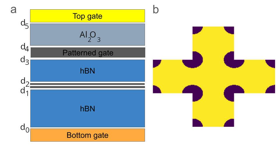
This device is general and can produce different physics. In order to simplify the analysis, for this thesis, we will keep the top and bottom layers fixed and vary the strength of the applied potential to the middle layer.
Solution to the Poisson equation
The coupling between the electrostatic potential and the electronic degrees of freedom is implemented following the procedure described in Sec. 1.
From (13) we can compute our occupations by integrating the DoS. For simplicity here, instead of using the KPM calculation for the density of states, we will use a simpler approach following the procedure shown in Appendix 8 where the DoS and LDoS are computed using a Green’s function method [Economou, 2006].
The only remaining ingredient is the explicit solution for the Poisson equation (46) in this device. The problem of solving the Poisson-Schrödinger equation in our 2D materials heterostack is reduced to
| (14) |
with the diagonal elements of the dielectric tensor, the dimensions considered on the and axes of the stack, and the Fourier transform of the potential and the electronic density, respectively. In Appendix 9, we give a detailed description of the derivation of this equation for a 2D material heterostack which can be done for an arbitrary choice of constant diagonal permittivities . In our case, we will choose the permittivity profile in to be:
| (15) |
where , are the average dielectric constants in and out-of the plane of hBN, respectively, and the average isotropic dielectric constant of . This is equivalent to assuming homogeneous media in Fig. 9 with sharp interfaces between different slabs.
The top and bottom gates are introduced as boundary conditions for and . For the patterned gate, on the other hand, a boundary condition treatment is not enough, given the reciprocal space nature of (14), we cannot easily discriminate between fixing the potential in some regions of space (graphitic regions) and allowing variations inside the holes. For that reason, our middle layer will be modeled as a capacitor where we will induce two surface charges in and in the interface between the graphitic gate and the dielectric. The surface charges potential are going to be
| parameter | Description | Value | ||
| top gate voltage | -580.5 meV | |||
| bottom gate voltage | -580.5 meV | |||
| patterned gate voltage | 487.5 meV | |||
| in-plane dielectric constant of hBN | 6.7 | |||
| out-of-plane dielectric constant of hBN | 3.56 | |||
| dielectric constant of | 9 | |||
| Lattice parameter of the middle gate | 20 nm | |||
| Diameter of the holes in Fig. 9 | ||||
| See Fig. 9 | -40 nm | |||
| See Fig. 9 | 0 nm | |||
| See Fig. 9 | 0.35 nm | |||
| See Fig. 9 | 5 nm | |||
| See Fig. 9 | 7 nm | |||
| See Fig. 9 | 27 nm |
| (16) |
with these absorbent surface densities, we guarantee that, for , the potential is homogeneous in the middle gate region. And, at the same time, we can expand its structure into the Fourier space, adding them as virtual charges in the equation (14). In Fig. 10 we can see the -profile of the potential in the stack and the effect of these charges in stabilizing a constant potential in the middle gate at before starting the convergence, so .

We have found a convergence up to for this system, in the inset of the bottom panel of Fig. 11 we can see the evolution of the convergence parameter. In this specific choice of parameters of Table 1, we can find well-defined quantum dots. That is, regions in space where the electrons are maximally confined.

In the dark region of the top left panel of Fig. 11 we can see the location of the quantum dots; this is the point where the local bands generated by (13) cross the Fermi level, while in the clear regions the system has the Fermi level inside the gap. This produces a characteristic localization of the quantum dots.
In the top right panel of Fig. 11 we can see the map of the potential difference in one superperiodic unit cell. Following the discussion of equation 13, the gap depends on , according to [Navarro Rodriguez, 2023], quantum dots are achievable with a difference in the gap so that the density of states is suppressed outside of the dot. On the other hand, in our case, the suppression generated by the non-homogeneous distribution of causes, even if the gap is maximal inside the dot, the energy shift generated by the distributions in the layer is enough to set the system inside (outside) the gap when outside (inside) the quantum dot.
In the bottom panel of Fig. 11 we can see the band-structure of the full superperiodic cell, and we observe that the dots’ bands present curvature. This is a characteristic of tunneling between different quantum dots [Navarro Rodriguez, 2023]. This interaction can be modulated depending on the strength of the potentials chosen or the distance between the dots.
With that, we have generated a superperiodic potential in a realistic device. These kinds of devices also present interactions, similar to those generated by the moiré systems, and can be used to engineer these interactions or study the physics generated by moiré in different interacting ranges [Barcons Ruiz et al., 2022].
Chapter 4 Transport in twisted Multilayer Graphene
Twisted multilayer graphene provides a natural route to engineering long-wavelength superlattices (moiré patterns) and, consequently, electronic states with strongly renormalized kinetic energy. In the magic-angle regime, the moiré bands become extremely narrow and the low-energy wave functions concentrate in the AA regions, creating an ideal setting where even weak perturbations can have an outsized impact on transport and localization. At the same time, real samples are inevitably affected by disorder (electrostatic fluctuations, local strain, and atomic-scale defects), which makes it essential to establish how robust the key single-particle fingerprints of twisted systems are against realistic perturbations before addressing interaction-driven phases.
This chapter applies the real-space transport framework developed earlier to realistic twisted graphene multilayers, with the aim of understanding how structural complexity and disorder reshape electronic propagation. The main focus is magic-angle twisted bilayer graphene, where the narrowness of the flat bands and the strong real-space modulation of the wave functions make transport especially sensitive to even weak perturbations. Within a single-particle, zero-temperature description, we quantify how Anderson disorder modifies the density of states, diffusion, and mean free path, and show that in a finite regime where flat-band features remain identifiable, moderate disorder can counterintuitively enhance transport through a disorder-induced delocalization mechanism.
We then connect this behavior to the evolution of the quantum metric extracted from optical conductivity, providing a geometric interpretation of the real-space extent of the electronic states. Beyond the magic-angle case, the chapter extends the analysis to graphene quasicrystal approximants and to hybrid trilayer stacks that combine moiré and quasicrystalline interfaces, allowing us to test the robustness of high-energy resonant and anomalous transport signatures against both disorder and proximity effects.
1 Computational details
Methodologically, we combine atomistic modeling of the relaxed geometries of twisted structures, a realistic tight-binding description of the full multilayer Hamiltonian, and linear-scaling KPM/real-space quantum-transport techniques to access large samples beyond direct diagonalization. Throughout the chapter, we characterize each system using the density of states, velocity renormalization, diffusion coefficients, and mean free paths, and we complement the transport analysis with geometric indicators (quantum metric) that connect naturally to the real-space extent of the electronic ground state and to the modern theory of localization.
1 Structural relaxation
To build realistic twisted graphene superlattices, we use molecular dynamics simulations with classical potentials to relax the structures [Guerrero et al., 2025b]. The importance of such relaxation procedures for the correct modeling of the electronic properties of twisted bilayer graphene for small angles has been reported in the literature [Nguyen et al., 2021, Nguyen et al., 2022]. However, for large angles, we have found an almost negligible difference between the relaxed and unrelaxed cases in our calculations [Guerrero et al., 2025a].
We start with uniform Bernal-stacked bilayer graphene, twisted to an angle of for the magic-angle and for the quasicrystalline approximants (see Sec. 1), and optimize the structure until all force components are smaller than 0.5 meV/atom. Intralayer forces are computed using optimized Tersoff and Brenner potentials [Lindsay and Broido, 2010], while interlayer forces are modeled using Kolmogorov-Crespi potentials [Kolmogorov and Crespi, 2005, Leven et al., 2016]. In reality, these materials are often deposited on substrates such as silicon oxide or encapsulated with other materials such as hexagonal boron nitride or stacked on top of graphite gates [Nguyen et al., 2022]. To model the effect of an underlying substrate, we force the flatness of the bottom layer of each stack not allowing relaxation in the vertical direction.
2 Tight-binding models
The electronic properties of the twisted multilayer systems are then computed using the tight-binding (TB) Hamiltonian,
| (1) |
where describes the orbital at the carbon site with position , is the electrostatic potential at the carbon site , and . The hopping energies between carbon sites are given by the standard Slater-Koster expression [Trambly de Laissardière et al., 2010, Nguyen et al., 2021].
| (2) |
where the direction cosine of along the -axis is . The distance-dependent Slater-Koster parameters are [Trambly de Laissardière et al., 2012]
| (3) |
with a smooth cutoff function . To model the flat electronic bands of relaxed TBLG at the magic angle , the TB parameters are adjusted to , , , , , , and [Nguyen et al., 2022].
3 KPM calculations
After relaxation of the lattices, we used a tiling magic-angle unit cell in our simulations, corresponding to atoms, to ensure a proper evolution of the electronic states and proper convergence of our methods. Similarly, for quasicrystalline approximants, a tiling of each unit cell, giving and for and approximants, respectively. For the trilayer, the same tiling was chosen, giving and for the and approximants.
After that, the KPM methods described in Sec. 2 were used to compute (local) densities of states, and the time evolution of the mean-squared displacement. Then, we followed a similar approach to the one described in Sec. 1 to extract the diffusion coefficient. For the time-evolving properties, a time step of was considered, evolving to in all our simulations. The only exceptions are the long-time calculations for clean systems, where we reached in order to find a precise description of the Fermi velocity and confirm the ballistic behavior of the system.
2 Magic angle twisted bilayer graphene
In this section, we present the results obtained for magic-angle twisted bilayer graphene, including the disorder-induced delocalization mechanism revealed in [Guerrero et al., 2025b].
1 Structural relaxation
From a structural point of view, we start with relaxed structures for the MATBLG. The effect of interatomic forces on the electronic properties of small-angle twisted bilayer graphene has been well established in [Koshino and Nam, 2020] and [Nguyen et al., 2022].
In these works, three different effects are clearly established:
- •
In-plane carbon atom displacements tend to reduce the size of the AA regions; this can be understood from the fact that, as we introduced in Sec. 3, AA graphene is less stable than AB graphene.
- •
This relaxation results in large out-of-plane displacements of the AA zones, increasing the interlayer distance in those regions. These can be viewed as frustrated regions.
- •
This relaxation effect is critical for the flat-band formation, helping to reduce the dispersion and is necessary to achieve a proper real-space modeling of the flat-band states.
We have relaxed our structure, achieving the described features. More specifically, we have replicated the results in [Nguyen et al., 2021], taking then the relaxed systems as a starting point for our electronic calculations.
2 Electronic structure
We start by analyzing the impact of disorder on the electronic structure of MATBLG through its impact on the total (DoS) and local density of states (LDoS). In Fig. 1 we plot the DoS for Anderson disorder strengths of , , and , where is the tight-binding parameter of graphene. For reference, we show the band structure of the clean case in the right inset and the LDoS at charge neutrality () in the left inset. The flat bands and the corresponding localization of the states in the AA regions are well reproduced in the absence of disorder. In the main panel, the presence of a strong peak in the DoS at highlights the presence of the moiré-induced flat bands. The role of disorder is to broaden and reduce this peak, which remains clearly visible at before finally being washed out for , coinciding with the disappearance of AA spatial localization (see the right inset of Fig. 5 for ).

3 Transport in the clean case
In Fig. 2 we show the spreading of the wave packet at short times, given by , where is the mean-squared displacement as defined in equation (7). We will follow a similar analysis as in Sec. 3 to bound the MSD with the characteristic length scales of the MATBLG. The top panel shows the clean case, and the bottom panel corresponds to a disorder strength of . On the -axis, the spreading of the propagation of the wave packet is shown in units of the moiré length of the MATBLG system, which is 13 nm.
In the clean case (top panel), at very short times, before reaching the first moiré length (ML), states propagate with the same velocity at all energies. However, upon reaching the first ML, the low-energy states in the flat band (red curve) undergo a dramatic slowing of their propagation velocity. In these states electrons are localized in the AA regions similarly to the left panel of Fig. 6 (see left inset of Fig. 1). The states adjacent to the flat band (yellow and green curves) experience a slowing at a spreading of 2ML. These states have been found to present antilocalization in the AA zone [Tong et al., 2022], similar to the right panel in Fig. 6. Meanwhile, the high-energy states (blue and purple curves) experience little velocity renormalization. In general, for the clean case, we observe a very similar transport behavior as the one observed for the superperiodic potentials of chapter 3, where the real-space pattern of LDoS behaves as a predictor for characteristic transport length scales.
In the disordered case (bottom panel), similar behavior is seen for the flat band (red curve), whereas states at all other energies converge to the same behavior owing to the Anderson disorder.
These results present a direct visualization of the accommodation of the wave function with the moiré lattice and the complex flat-band physics of MATBLG. They also provide lower spatial and temporal bounds for the appearance of such flat-band physics, which do not appear until the wave function has evolved long enough to see the superperiodicity of the moiré lattice. This also remarks that the inherent physics of superperiodic transport studied in the previous chapter only happens at the energies of the flat band, confirming the difference against transport between inter- and intra-layer states presented in Sec. 4.

In Fig. 3 we plot the long-time evolution of the diffusion coefficient of clean MATBLG. In the absence of disorder, the transport is ballistic and the diffusion coefficient increases linearly with time . This behavior is seen at all energies (different colored curves) in Fig. 3. From the slope of these curves we then extract the Fermi velocity of the MATBLG system, which we plot in the inset, relative to the velocity of single-layer graphene . Note that while the Fermi velocity may not be uniform around the Fermi surface, here we plot its average over the Fermi surface at the indicated energies . Here we see that around charge neutrality the Fermi velocity is very low , characteristic of the flat nature of the moiré bands.

4 Disorder-induced delocalization
We use this section to study the weakness of the MATBLG localized states against disorder. In Fig. 4 we examine electronic transport in disordered MATBLG. In the presence of Anderson disorder, the diffusion coefficients now saturate at long times for all energies. However, we observe a qualitative difference between transport within the flat bands compared to that at higher energies. When increasing the strength of the disorder from , decreases by a factor of for all energies except at charge neutrality (red curve), where actually increases, opposite to typical behavior. This is illustrated further in Fig. 5, where we plot the mean free path for three different strengths of the disorder. In the energy range corresponding to the moiré flat bands, for weaker disorders we see a clear increase of the mean free path with increasing disorder strength, opposite to the scaling behavior at higher energies. This increase in actually coincides with a delocalization of the LDoS around charge neutrality in the presence of disorder, as highlighted in the left and right insets of Fig. 5. 11 1 Here we note a slight electron-hole asymmetry in the mean free path, arising from an asymmetry in the band structure (inset of Fig. 1) and correspondingly in the Fermi velocity (inset of Fig. 3). A similar behavior of the electron-phonon coupling in MATBLG has been reported in Refs. [Choi and Choi, 2018, Gadelha et al., 2022]. This disorder-induced delocalization was later found in a qubit array quantum simulator [Rosen et al., 2025], and in other theoretical works [Hou et al., 2025].

We note that a stronger disorder will eventually suppress any remnant of the flat bands and thus reduce the mean free path following the scaling behavior , where is the carbon-carbon spacing. This is seen when the disorder increases from to in Fig. 5.
Therefore, the observed anomalous “disorder-induced delocalization” exists over a finite range of disorder strengths and is maintained when disorder is low enough to preserve the moiré-induced flat-band states. This effect is driven by the disorder-induced broadening of the flat bands and the corresponding delocalization of states in real space. Using a simple argument based on the Fermi golden rule, the increase in the mean free path is driven by the reduction of the DoS and the corresponding scattering rate. For weaker disorder, following the scaling theory of localization, one expects that near flat bands the localization length (related to the mean free path through the Thouless relationship) will reach values on the order of 100 nanometers for a disorder strength corresponding to the effect of electron-hole puddles generated by a silicon oxide substrate [Van Tuan et al., 2016]. Finally, we note that in the strong Anderson disorder limit, the mean free paths in disordered MATBLG are similar to those found in disordered monolayer graphene [Lherbier et al., 2008].
5 Impact on quantum metric and correlations
To compute the quantum metric, we make use of the SWM rule [Souza et al., 2000], which relates it to the optical conductivity (via the fluctuation-dissipation theorem) as
| (4) |
where is the dimensionless quantum metric, is the electric charge, is the Planck constant, is the optical conductivity, and is the frequency. This QM is related to the invariant part of the spread of the Wannier functions [Marzari et al., 2012], , where the trace runs over the Cartesian indices. Here, a small QM relates to a small Wannier spreading, and thus to a strongly localized ground state. On the other hand, when the QM continuously increases with system size, it indicates delocalization of the Wannier functions and the ground state. Here we compute from the Kubo formula [Kubo, 1957], making use of a Chebyshev polynomial expansion [João et al., 2020] with a broadening of 66 meV, and obtain convergence of with system size and number of polynomials.
Fig. 5 (bottom panel) shows for different strengths of the disorder, and we compare its disorder-dependent evolution with the mean free path. Interestingly, the evolution between and is qualitatively similar for and , indicating a disorder-induced delocalization mechanism. The increase in QM at lower disorder is expected for weakly disordered cases, since the cleaner the system, the longer the corresponding mean free path and localization length. Note that the precise value of the mean free path is not shown for the lowest disorders due to computational difficulty accessing the diffusive regime in the simulations. However, we can make a rough estimate using the Fermi golden rule when disorder only weakly affects the band structure, for which . Taking the smallest value of the disorder with a converged mfp (), for which nm, we extrapolate nm for and nm for .
![[Uncaptioned image]](/html/2607.25411/assets/figures/Mean_free-path-deloc.png)
Here it is important to note that such disorder-induced changes in the integrated quantum metric could also have an impact on MATBLG superconductivity and the superfluid weight of the states following some recent works relating the contribution of the integrated quantum metric to the superfluid weight and the critical temperature [Julku et al., 2020, Törmä et al., 2022].
3 The graphene quasicrystal
1 The quasicrystal approximants
As we saw in Sec. 4, a quasicrystal has, by definition, no real-space periodicity. In Sec. 4 we faced the difficulties of studying transport with open boundary conditions. Due to computational limitations, the system sizes studied for twisted bilayer graphene do not achieve the real-space extension of the superimposed potential artificial moirés displayed in chapter 3. There are several other strategies one could follow to mitigate these effects, such as the use of absorbing boundary conditions [Mandelshtam and Taylor, 1995, de Castro et al., 2023, de Nova et al., 2024].
In our case, with the purpose of avoiding contamination of our results from the boundary conditions, we will rely on the quasicrystal approximants. This is a common approach [Goldman and Kelton, 1993, Moon et al., 2019] in the quasicrystal community where the aperiodic structures are approximated for increasingly similar, longer periodicity systems. More specifically, we will approximate our graphene quasicrystal with two levels of approximation, the and angles that have unit cells of sizes and respectively.
2 Structural relaxation results
We report that the results obtained for structural relaxation in the two systems under study are negligible both from the in-plane and out-of-plane displacements. The impact of such relaxation is also negligible from an electronic point of view. This lack of relaxation was previously predicted for large angle twisted graphene bilayers [Nguyen et al., 2022] as a result of the homogeneity of its stacking where there are no long-range AA or AB zones.
As a result, we have carried all our calculations in relaxed structures for the quasicrystal approximants, but confirm that these results are independent of the structural relaxation.
3 Transport in the clean case

In the top left panel of Fig. 6, we can see the density of states of the and approximants, where we see has a much closer DoS to the one expected for the quasicrystal (See the resonant states of Fig. 9). In we can clearly distinguish the resonant states associated with the (purple), (green), and (orange) marked as the three vertical lines.
In the bottom left panel, we can see the diffusion coefficient at very short times, here we have considered the times before the electronic spreading reached the superperiodicity of the approximant, so we have only considered times . The transport within this constraint shows a clear difference between the states in and outside the resonant peaks. In the purple, green, and orange curves, we see how the transport at the resonant peaks presents sub-ballistic features, confirming the quasicrystalline nature of those states. For all three, we have predicted similar values for the exponent of thus providing, to our knowledge, the first estimate in the literature for the sub-ballistic exponent of the dodecagonal graphene.
In the three panels on the right of Fig. 6, we see confirmation of the quasicrystalline nature of these states, achieving for and quasicrystalline states that follow inflations of the Stampfli pattern, as we already introduced in Sec. 2 and was shown in other results in the literature[Vidarte and Lewenkopf, 2024, Ahn et al., 2018].
4 Weakness against disorder
Disorder-induced delocalization, in a way similar to how it was introduced for magic-angle twisted bilayer graphene in Sec. 4, is a longstanding conundrum for studies based on intermetallic-alloy quasicrystals. Based on the results presented in that section, we can infer that such delocalization could be caused by the breaking of the subtle fractal ordering offered by such quasicrystals due to the addition of these new disordered states.

We try here to identify this disorder-induced delocalization within our limitations for the quasicrystalline approximants. In the left panel of Fig. 7 we can see the diffusion coefficient for disorders of and of the states present in peak of dodecagonal graphene. At a specific choice of disorder, for all times, transport is always decreasing for increasing values of disorder, not showing this exotic feature, and instead following the usual Fermi golden rule. Note that we extended the calculations to smaller disorders than those studied for the magic-angle case of Sec. 4, where, as we stated, for monolayer graphene produces mobilities similar to those induced in graphene by electron-hole puddles of an hBN substrate.
We can see the reason in the bottom panel of Fig. 7 where the local density of states of dodecagonal graphene is displayed. We observe that the -peak localization pattern present in Fig. 6 has vanished for . This is a sign of the weakness of such quasicrystalline states against disorder and predicts that the resistive features of quasicrystals can only be observed in extremely small disorders.
However, it is also important to make two considerations here regarding the limiting factors for our calculations:
- •
The amount of disorder that we can achieve with precision in our calculations is lower bounded due to the finite size of our systems and the presence of an electronic broadening in the electronic states. This implies the possibility that this system can present disorder-induced delocalization mechanisms at extremely weak disorders .
- •
As we saw in Fig. 6, as a result of the use of approximants, we observe traces of the resistivity of quasicrystals in transport only at relatively short distances (below the superperiodicity). Loss of the localized fractal picture is not expected to be limited by the approximant unit cell, but to evolve continuously towards the formation of the fully -fold symmetric states. Yet we remark that more studies with larger approximants are needed in order to completely discard the delocalization induced by disorder.
4 A trilayer with quasicrystal and magic-angle
So far, we know that: (i) in magic-angle twisted bilayer graphene (MATBLG), interlayer hybridization at small twist produces low-energy flat bands and associated transport anomalies (Section 2), and (ii) in twisted bilayer graphene the strongest hybridization is shifted to high energies and gives rise to resonant quasicrystalline states with characteristic dodecagonal real-space patterns (Section 3). A natural next step is to combine both ingredients in a single stack and ask whether the two energy sectors remain effectively decoupled, or instead imprint measurable proximity effects on one another.
In this section, we therefore consider a trilayer hybrid heterostructure in which a MATBLG bilayer is interfaced with a graphene quasicrystal approximant (near ), following the large-scale tight-binding and real-time Kubo simulations. Because the relevant phenomena live at well-separated energies (flat-band physics in the - window around charge neutrality versus quasicrystalline resonances in the – range) the analysis is most transparent when organized into a low-energy and a high-energy regime. We will first examine how the additional layer at affects the spectral fingerprints and transport of the flat bands, and then turn to the high-energy quasicrystalline peaks and their anomalous dynamics.
For that, in the rest of this section, we set a angle rotation in the bottom and middle layer interface; and a rotation in the middle to top interface.
1 Structural relaxation

Similarly to the previous sections, for our electronic calculation, the displacements on the axis of the bottom layer are fixed to mimic the effect of a substrate. However, we want to make a further comment here on the relaxation in the trilayer. We observed a dominance in the structural relaxation of the QC+MATBLG trilayer of the -zones in the twisted interface.
In Fig. 8 we observe the difference in the out-of-plane displacements between the relaxation of the full bilayer when the bottom layer is set free (left panel) and when it is fixed in the out-of-plane coordinates. In the free case, we observe the impact of the MA interface (middle and top layers), where the out-of-plane displacements in the regions of this interface tend to increase the interlayer distance between the middle and top layers, while the interlayer distance between the two bottom layers remains almost constant. This is maintained in the bottom layer, where these regions present a displacement that keeps the interlayer constant approximately close.
In contrast, when we fix the out-of-plane displacements of the bottom layer to zero, the interface also forces the flatness of the middle layer, as we can see from the right-hand panel of Fig. 8 where the vertical displacements can be considered negligible.
However, we found no significant differences in the electronic structure or transport in the initial calculations and decided to choose the Fixed version because of experimental relevance.

2 The low-energy regime
We now turn to the low-energy window, where the electronic structure of magic-angle twisted bilayer graphene (and in our trilayer) is dominated by the moiré flat bands discussed in Sec. 2.
DoS and averaged Fermi velocity.
Fig. 9 compares the DoS of MATBLG (reproduced from Fig. 1) in purple; with that of the two trilayers built from the and quasicrystal approximants in dashed and solid black lines, respectively. Here, within the flat-band window , the DoS remains essentially unchanged when the quasicrystalline layer is added: the low-energy peak associated with the moiré flat bands remains nearly identical in the bilayer and trilayer stacks. At somewhat larger energies, a modest increase in DoS appears in the trilayers, consistent with the emergence of additional dispersive channels provided by the extra graphene layer [Guerrero et al., 2025a].
The bottom panel of Fig. 9 shows the corresponding energy-dependent Fermi velocity, extracted from the ballistic scaling of the diffusion coefficient. Although the DoS suggests that the flat bands themselves remain intact in the clean limit, the averaged Fermi velocity can increase substantially in the trilayer, reaching factors of in the most severe cases. Importantly, this increase does not necessarily imply a genuine steepening of the MATBLG flat bands: since the velocity is averaged over the full Fermi surface, it can reflect parallel transport through a largely decoupled quasicrystalline layer with a graphene-like velocity scale. To disentangle these effects we introduce a “decoupled” control calculation in which the interlayer hoppings between the MATBLG bilayer and the third layer are removed, mimicking an infinite separation between the layers. The resulting curve (red in Fig. 9) shows that, at low energies, both the DoS and the averaged velocity remain essentially unchanged relative to the coupled trilayer. This supports the interpretation that the low-energy flat-band manifold is only weakly hybridized with the layer in the pristine case, and that the apparent velocity enhancement is dominated by the additional conducting channel rather than a strong modification of the MATBLG states.
Layer-projected spectral weight and LDoS at charge neutrality.

The weak hybridization picture is further corroborated by the layer-resolved quantities in Fig. 10. The layer-projected DoS demonstrates that the flat-band peak is carried almost entirely by the two -twisted layers (the MATBLG bilayer), whereas the layer contributes a spectrum that resembles that of (nearly) monolayer graphene. Consistently, the LDoS maps reveal the characteristic moiré periodic modulation in the MATBLG layers, with increased weight in the AA overlap regions as discussed in Sec. 1 and 2, while the quasicrystalline layer shows no imprint of the moiré superlattice at low energy. Altogether, Fig. 10 indicates that the third layer behaves largely as a spectator in the clean low-energy regime: it provides additional (graphene-like) states, but does not absorb spectral weight from the MATBLG flat bands.
Disorder and the suppression of disorder-induced delocalization.

We now test whether this apparent resilience extends beyond spectral properties by introducing Anderson disorder, as in Sec. 4. We consider the same disorder strengths as in that section and and compute the time-dependent diffusion coefficient at the center of the flat band (). For MATBLG alone, the inset of Fig. 11 (adapted from Fig. 4) presents the anomalous trend previously reported and discussed in Sec. 4: at long times, increasing disorder can lead to an increase of the diffusion coefficient.
Interestingly, this behavior is reversed in the trilayer stack. As shown in the main panel of Fig. 11, once the quasicrystalline graphene layer is added, the diffusion coefficient follows a conventional trend: a larger disorder systematically reduces at long times, consistent with standard disorder-limited transport. This occurs despite the fact that, in the clean limit, the low-energy states remain strongly projected onto the MATBLG layers. We attribute this difference to the new electronic channels enabled by the presence of the extra layer twisted that enables the scattering of states from the MA interface in the presence of disorder.
We want to remark that at very short times this disorder-induced delocalization (see left white region of Fig. 11) can be recovered and even increased for shorter times. For other times, the scaling from Sec. 4, where for increasing disorder we find delocalization localization, can be recovered (gray region of Fig. 11). This predicts that for a sufficiently short sample these effects could be observed even in our trilayer.
3 High-energy states

We now turn to the high-energy window where -twisted bilayer graphene (tBLG) quasicrystals display their most distinctive electronic fingerprints in the shape of a set of resonant peaks in the energy range. Fig. 12 summarizes the main impact of the proximity effect with the layer in this energy range. For the quasicrystalline bilayer approximants, the DoS shows prominent resonant structures, and we single out the peak at (vertical line). Remarkably, when the magic-angle bilayer is brought into proximity, forming the trilayer, these resonant fingerprints are strongly suppressed: the DoS becomes significantly smoother and the corresponding Fermi velocity profile turns comparatively featureless. Instead of resonant peaks, the combination between the quasicrystal and the -rotated layer induces a systematic reduction in velocity throughout the high-energy range of interest, consistent with an enhanced hybridization background but a strong degradation of the quasicrystalline resonant response.

The same conclusion emerges from the probes in real space. In the pristine quasicrystalline bilayer, the LDoS evaluated at the peak displays a highly inhomogeneous, self-similar localization landscape (left panel of Fig. 13), reflecting the emergence of a dodecagonal order that is incompatible with translational invariance, as we previously saw in Fig. 6. In sharp contrast, evaluating the LDoS on the same atomic coordinates for the bottom and middle layers (quasicrystalline interface) within the trilayer, we observe that this fractal localization pattern is destroyed and replaced by a much more homogeneous distribution. This highlights a key qualitative asymmetry of the proximity effects explored in this section: while low-energy flat-band physics can remain comparatively robust to adding a quasicrystalline layer in the clean limit, the high-energy quasicrystalline states are instead fragile to the presence of a magic-angle layer.

Transport simulations reinforce this picture. Fig. 14 compares the time-dependent diffusion coefficient at the -peak energy for the quasicrystalline approximant and the trilayer. In the inset, we can see a comparison between the short-time behavior of the quasicrystalline bilayer (blue curve, extracted from Fig. 6) and trilayer (black). Surprisingly, the quasicrystalline resistivity was washed out even in this pristine case, where the states are now conventional ballistic states.
Introducing Anderson disorder drives both systems into standard diffusive behavior in this high-energy regime: increasing the disorder strength monotonically reduces and shortens the effective mean free path. Here, with the addition of disorder, the transport in the bilayer and the trilayer cannot be distinguished from each other.
The combination of these results supports a central idea: The broadening of the states induced by the sole proximity of the layer is strong enough to mix the resonant states, whose fragility to disorder we spotted in Sec. 4. Creating a region of the space with a reduced Fermi velocity as a result of the impact of the resonant states of the pristine bilayer but with no signature of quasicrystalline features itself. With the addition of disorder, the broadening induced by the extra layer becomes negligible compared to the broadening induced by Anderson disorder, and the transport becomes indistinguishable between the tri- and bilayer.
Chapter 5 Magnetism in Twisted bilayer Graphene
In Sec. 1 we saw that one of the most important aspects of MATBLG comes from the discovery of highly correlated phases. There, the emergence of narrow moiré bands in MATBLG places the system in a regime where Coulomb interactions compete on the same footing with kinetic energy, allowing for a complex phase diagram in the presence of exotic phenomena such as the correlated insulator or the superconductor phases. [Cao et al., 2018b, Cao et al., 2018a, Balents et al., 2020].
These observations motivate a microscopic characterization of magnetic ordering tendencies in moiré flat-band systems, and provide a concrete arena where spin, valley, and sublattice degrees of freedom intertwine with topology. As we discussed previously in Sec. 2 a simple study of these magnetic properties can be understood as a first approach to the electron-electron correlations.
This chapter provides an exploratory extension of the thesis from transport and localization toward interaction-driven physics in magic-angle twisted bilayer graphene. In particular, it focuses on magnetic and topological phases reported experimentally in this platform and on the microscopic modeling strategies commonly used to describe them. The purpose of Chapter 5 is not to present a complete theory of correlated magnetism, but rather to establish the first steps toward incorporating electron-electron interactions into the real-space framework developed in the previous chapters. The motivation is to eventually jointly address the impact of disorder and Coulomb interaction (limited to a treatment in the mean-field approximation) on the delocalization-localization effects we have found in Chapter 4. Indeed, if the measured cleanest samples of twisted bilayer graphene at magic angles clearly exhibit highly exotic physics that clearly demand to go beyond the mean field, the physics of lower-quality samples (presence of twist angle disorder, electron-hole puddles, proximity effect,..) might be partly captured by a mean-field approach due to the disorder-induced broadening of flat bands, and thus reduction of local electron-electron interaction strength. Additionally, the presence of fragile magnetic states in part of the phase diagram has also been the focus of intense studies, whose origin remains debated.
In that sense, this chapter serves as a bridge between the single-particle transport perspective of the previous one and the broader problem of how disorder, flat-band localization, and many-body instabilities may interplay in moiré systems. Because this part of the project remains computationally challenging, the discussion is necessarily more programmatic and methodological, but it clarifies both the physical motivation and the limitations that define the next stage of the research.
1 A landscape of exotic phases
This section reviews the advances in the study of correlations for magic-angle twisted bilayer graphene achieved to date, as well as their main results concerning the onset of magnetic ordering.
1 Experimental phenomenology: from anomalous Hall response to quantized Chern insulators
In the first experimental reports on MATBLG, Cao et al. already revealed a close proximity between the insulating and superconducting ground states as a function of carrier density [Cao et al., 2018a, Cao et al., 2018b]. Shortly thereafter, transport experiments uncovered clear signatures of magnetic ordering in parts of the moiré phase diagram. A particularly direct indicator is the appearance of a large anomalous Hall response accompanied by hysteresis, consistent with a ferromagnetic state that breaks time-reversal symmetry. In 2019 Sharpe et al. reported emergent ferromagnetism near the three-quarter filling of a moiré miniband, together with a giant anomalous Hall effect and current-driven switching of the magnetic state [Sharpe et al., 2019]. Although the Hall response in that work was not quantized, it suggested that MATBLG can realize an incipient Chern-insulating regime when interactions polarize the relevant internal degrees of freedom.
A decisive step towards topological magnetic order came with the observation of a robust quantized anomalous Hall (QAH) effect at (effectively) zero magnetic field. In devices where MATBLG is crystallographically aligned with hexagonal boron nitride (hBN), Serlin et al. observed a Hall resistance quantized consistent with a Chern insulator around 3/4 filling of the flat band and accompanied by ferromagnetic order [Serlin et al., 2020]. Importantly, the QAH response was shown to be electrically switchable with extremely small currents, emphasizing the unusually soft magnetic energy scales typical of moiré flat-band systems.
Subsequent experiments have broadened this picture, revealing that correlated topological phases in MATBLG are not limited to a single filling factor or a single device architecture. Gate-tunable Chern insulating states with different Chern numbers have been reported near several integer fillings, often in close competition with superconducting domes or other correlated insulators [Stepanov et al., 2021]. Thermodynamic and transport probes further indicate that flavor symmetry breaking is a recurring motif at integer fillings, and that a “Hund-like” energetic hierarchy between spin/valley flavors can influence the gap formation and the anomalous Hall response [Park et al., 2021]. Scanning probe and compressibility measurements have also revealed an unexpectedly rich sequence of incompressible states, including phases interpreted as correlated Chern insulators and, at finite fields, fractional Chern insulators emerging from moiré Chern bands [Pierce et al., 2021, Xie et al., 2021].
Taken together, these observations suggest that magnetic order in MATBLG is often entangled with band topology and with the multi-component (spin/valley) structure of the moiré bands. The experimental phase diagram is therefore best viewed not as a single ordered state but as a landscape of competing instabilities whose energetic separation can be comparable to disorder, strain, screening, and small symmetry-breaking fields. The question of how disorder influences and impacts this landscape, where subtle changes in the occupations can substantially reshape the observed ordering tendencies remains an open question, and even if current techniques don’t allow us to address this problem in all its complexity, it motivates first studies on the effects of disorder on the description of such magnetic states.
2 A mean-field approach to correlations
From a theoretical point of view, the natural starting point for most works is the continuum description of moiré bands using a Bistritzer-MacDonald (BM) model that can be considered a generalization of the one presented in (13) [Wu et al., 2018, Bistritzer and MacDonald, 2011]. While the BM framework is fundamentally a single-particle theory, its ability to capture the formation of extremely narrow bands makes it an ideal platform to investigate correlation effects either by adding interactions at the mean-field level or by constructing effective low-energy lattice Hamiltonians where many-body methods can be applied.
One of the most direct strategies is to incorporate Coulomb interactions in the continuum model through self-consistent Hartree or Hartree-Fock (HF) approximations. These approaches exploit the fact that the moiré wave functions have strong real-space modulation, which enhances exchange and can naturally drive flavor symmetry breaking (spin/valley polarization, intervalley coherence, etc.). In this spirit, continuum HF calculations have been used to account for correlated insulating behavior at commensurate fillings and to map out competing broken-symmetry states as a function of filling and interaction strength. First, Liu et al. [Liu and Dai, 2021] found an antiferromagnetic phase with a bandgap of , qualitatively in agreement with the measured gap of . In [Zhang et al., 2020, Bultinck et al., 2020] this gap is predicted to be on the order of meV. The key message emerging from these studies is that in MATBLG, the energetic hierarchy between different ordered states can be extremely small, so that weak perturbations (substrate alignment, strain, screening environment, displacement fields) may play a decisive role in selecting the experimentally realized phase.
A real-space perspective becomes particularly valuable when discussing magnetic textures and spatial inhomogeneity of the order parameter within the moiré unit cell. The methods for these self-consistent algorithms are similar to the ones described in Sec. 2 which differ in the computation of the local density of states. In this direction, Vahedi et al. made use of Green’s function recursion to simulate the real-space HF (as the one presented in Sec. 2) both with mean-field theory (MFT) and with dynamical mean-field theory (DMFT) [Georges et al., 1996]. With that, they could investigate magnetic instabilities close to charge neutrality [Vahedi et al., 2021]. These studies show how different approximations (HF, DMFT) support the formation of magnetic trends. The simplest approximations (as the one generated by a HF) proved to result in the same antiferromagnetic phases at zero filling of the band-gap, while differing on quantitative parametric values in the interactions for achieving similar magnetizations.
In that line, Vidarte et al. [Vidarte et al., 2025] used a similar approach with a combination of Lanczos-like [Haydock et al., 1972, Haydock et al., 1975, Haydock, 1980] real-space spectral calculations and HF, finding both the presence of anti-ferromagnetism at zero filling of the flat band and a ferromagnetic phase at 3/4 filling of the flat band, potentially inducing Chern phases similar to the ones predicted by Serlin et al.
At zero filling Vidarte et al found antiferromagnetism with local values for the gap in the AA zones in the order of magnitude of for a Hubbard parameter ratio and at filling, they found ferromagnetic gaps up to .
2 Mean-field simulations
In the following sections, we follow the steps of Vahedi and Vidarte [Vidarte et al., 2025] with our KPM approach and target a mean-field convergence by making use of the algorithm described in Sec. 2, with the objective of studying such magnetic phases under disorder. To do so, we will make use of our KPM approach to compute local densities of states as shown in (33).
1 The structural relaxation
The original study by Vidarte et al. showed results for a relaxed and an unrelaxed structure. In a similar fashion, for relaxed cases, we have considered both the fixed and the free bottom layer with the computational details given in Sec. 1.
2 Tight-binding model
In order to obtain results as close as possible, we use the tight-binding model proposed in [Vidarte et al., 2025, Vidarte and Lewenkopf, 2024], defined as
| (1) |
with
| (2) |
This can be understood as a version of (2) with slightly modified exponential decay. The parameterization of the model is reported in Table 1. In Fig. 2 (See section 2), we showed that this model and the one used in (2) give very similar results.
| parameter | Description | Value | ||
|---|---|---|---|---|
| -bond transfer integral at equilibrium | ||||
| -bond transfer integral at equilibrium | ||||
| in-plane nearest-neighbor average distance | Å | |||
| out-of-plane nearest-neighbor average distance | Å | |||
| decay length | 0.319 |
This model precisely reproduces the flat band and the electronic localization in the AA zones of the MATBLG shown in Fig. 1.
3 Computational details
To date, our KPM approach has not been able to reproduce the results shown by other real-space studies that report magnetizations in the range of 0.1-10 meV for a wide variety of values of the Hubbard parameter [Vahedi et al., 2021, Vidarte et al., 2025]. For this reason, we report the computational details of the calculations carried out so far and provide a careful discussion of the possible origins of these discrepancies. Following the steps of the two articles cited, we have considered two different twist angles for our calculations, and and, for each of them, two different fillings of the flat band , with expected antiferromagnetic and ferromagnetic states, respectively. In order to achieve sufficient precision, we have chosen tilings of the unit cell of , formally equivalent to the -point mesh grid considered in [Vahedi et al., 2021]. For the twist angle we were unable to achieve the precision required for the LDoS calculation of such a large lattice in a reasonable amount of computational time, so the tilings are as large as times the unit cell. For the energy broadenings we have taken a constant value of , narrower than the regularization parameter considered in [Vidarte et al., 2025] for the Lanczos recursion. Meanwhile, the number of moments at each iteration changes in order to keep this broadening constant according to (27). The energy step considered for the integral is , orders of magnitude below the minimal gap considered for the two previous works.
4 Initial conditions
In order to conduct the self-consistent procedure exposed in Sec. 2, we need to make a choice of the initial conditions for step 2. Here, we have considered three possible initial conditions for magnetization.
- •
Random initial conditions: we initialize all magnetizations with a uniform distribution of random values in the range .
- •
Antiferromagnetic initial conditions: We induce an antiferromagnetic phase localized in the AA zones, where the magnetization is set to where is the decay length and with positive (negative) sign assigned to the A (B) sublattice.
- •
Ferromagnetic initial conditions: We initialize all lattice sites to a finite magnetization .
After setting the magnetizations, the initial occupations are computed as
| (3) |
with the number of lattice sites in the unit cell.
5 Results
Several values have been reported in both [Vahedi et al., 2021] and [Vidarte et al., 2025]. The configurations are similar, both in the potential and in geometry, having the second case also considered relaxed lattices. Both articles first discuss the angle as a simple case and then focus on the magic-angle. We have tried to run convergences in both and where, at the time, we have not achieved the proper convergence in either of the cases. In general, we see both the convergence parameter and magnetization at all lattice sites decrease as the convergence steps increase. In Fig. 1 we can see an example of convergence behavior where the magnetizations at each site reach values smaller than the tolerance in our convergence criterion. We report here only the results related to because of the simplicity in their treatment, together with the dimensionless magnetizations
| (4) |
Overall, both articles show good qualitative agreement in their results. However, we can spot some differences between them. In [Vahedi et al., 2021], they report a critical value for of , while in [Vidarte et al., 2025] the system clearly shows magnetization on the order of , showing a band-gap in the AA dimer sites of . A smaller gap between spin channels is reported in the AA dimer site in [Vahedi et al., 2021] in the case of with a reported larger magnetization .
The combination of these results suggests that the critical energy splitting between states could be highly dependent on the simulation method. We consider here some plausible reasons for the failure to achieve satisfactory convergence and future routes to achieve precise results:
- •
Effect of the broadening. The precision of KPM is known to be highly dependent on its broadening [Fan et al., 2021]. The broadening within our computational capabilities, as small as , could not have been precise enough to achieve satisfactory resolution of such small differences in spin channel occupations. In addition, the Jackson kernel broadening we use does not generate a uniform broadening along the whole unit cell, and it is possible that the effective broadenings in the flat band are smaller than what we report here given the electron-hole asymmetric nature of the problem. To mitigate that, we have also considered the Lorentz kernel [Fan et al., 2021] with similar results for both kernels.
- •
Numerical error. We acknowledge that the techniques involved in the proposed algorithm are highly sensitive to numerical precision and the coordination of two different self-consistent methods. Any uncontrolled numerical instability during the calculation could be a source of randomness large enough to remove the spin imbalances between channels.
- •
Finite-size effects. The feasibility of this work depends on finding a good compromise between computational time and accuracy. For that, we have considered grids up to replications in real space. This number is chosen to consider a similar number of bands as [Vahedi et al., 2021] while [Vidarte et al., 2025] does not report the exact real-space tiling of their calculations. We have compared our densities of states in the unperturbed case and considered that it converged sufficiently compared to tilings, but the cumulative error during the convergence could be too large to achieve correct results.
- •
The energy grid. To maintain reasonable amounts of computational time, we have chosen energy grids spaced . Small differences in the exact point of the Fermi level could lead to a lack of detection. We have tried to refine this energy grid at the expense of some precision in terms of broadening, but the results were not satisfactory.
In Figs. 1 and 2 we can see a typical convergence for the mean-field problem for the 0 filling and 3/4 filling of the flat band. Here we observe the convergence of a twisted bilayer graphene with a twist-angle of .
It is clear that the magnetization (left panels in Figs. 1 and 2) reaches values compatible with the precision (we recall here that our convergence parameter is the difference between two consecutive steps) with no clear indicators of convergence. In contrast, in the upper left panel of Fig. 3, we observe a typical convergence behavior of the problem. Despite the lack of convergence, in the right panels of Figs. 1 and 2 we observe a qualitative distribution of the local magnetizations similar to the one expected from [Vahedi et al., 2021, Vidarte et al., 2025].


6 Validity of the method
To better understand the effects of the broadening, one can present an easier problem concerning zig-zag graphene nanoribbons (zGNR). In Fig. 3 we observe a convergence of the KPM-mean-field calculation for a zGNR, computed with the same method that was used for section 5. In the top and bottom right panels of Fig. 3 we observe the converged results for the magnetization of the zig-zag graphene nanoribbon in its ferro- and antiferromagnetic phases respectively, computed for a broadening of meV. These results are qualitatively correct when compared to previous results in the literature [Moles et al., 2025], while quantitatively underestimating the magnetizations. In the upper left panel, we can see that the self-consistent algorithm is properly converged for these results.
In the bottom left panel, we observe the predicted maximum local magnetization for antiferromagnetic (green) and ferromagnetic (orange) solutions. We note that the quantitative values for these local magnetizations show a strong dependence on the broadening. This suggests that the effect of the broadening may be substantial in KPM calculations and that further optimization is needed, which is currently beyond our computational capabilities. Yet, we note that this subtle dependence on the broadening of the states can be achieved by disorder-induced broadening and suggests a large variation of magnetization for these flat-band systems against small amounts of disorder.

Chapter 6 Spin transport in corrugated monolayer graphene
This chapter turns to spin transport in suspended monolayer graphene, using it as a complementary setting in which structural complexity affects dynamics in a way that differs markedly from charge transport. After reviewing the basic spin-orbit coupling terms relevant to graphene and the main semiclassical mechanisms of spin relaxation, the chapter introduces an atomistic description of thermally corrugated graphene in which local curvature generates position-dependent hopping, doping, and spin-orbit fields. Realistic corrugation profiles are obtained from molecular-dynamics simulations, and these are combined with a curvature-dependent tight-binding Hamiltonian to study both charge diffusion and spin dynamics.
A central result is that atomic-scale corrugations leave charge transport comparatively close to the ballistic regime over broad energy windows, while simultaneously producing strong short-range fluctuating Rashba fields that drive efficient spin relaxation and limit spin lifetimes to the nanosecond scale. In this way, the chapter shows that spin transport is an especially sensitive probe of microscopic structural disorder and provides a concrete mechanism to reconcile the high mobility of suspended graphene with the much shorter spin lifetimes observed experimentally.
1 Spin-orbit coupling in graphene
This chapter mainly follows the work developed by Fabian et al. in [Fabian et al., 2007]. We start our work by introducing a simple low-energy model for spin-orbit coupling (SOC) in graphene. We will consider intrinsic and extrinsic contributions to the spin-orbit coupling. In pristine free-standing graphene the intrinsic SOC is very weak due to the small atomic number of carbon and the planar bonding environment [Huertas-Hernando et al., 2006]. However, there are many other contributions to SOC that can arise in proximity to other materials [Song et al., 2018].

Starting with the intrinsic SOC, one can consider the usual interaction between spin and orbit, the Kane-Mele spin-orbit coupling [Kane and Mele, 2005]. This is an intrinsic SOC generated by the symmetries of the honeycomb lattice: it is the only spin-dependent term allowed by time-reversal symmetry, inversion symmetry between the two sublattices, and the threefold rotational symmetry of graphene, and it manifests itself as a next-nearest-neighbor spin-dependent mass term that preserves all lattice symmetries.
| (1) |
Microscopic tight-binding calculations show that in monolayer graphene [Konschuh et al., 2010] is extremely weak. Under typical conditions, eV is found in clean graphene [Gmitra et al., 2009]. We can see the effect of this term on the band structure of the top right panel of Fig. 1. There we can see that it produces a topological gap that can then be experimentally measured [Sichau et al., 2019]. Experimental works have found that it has a value of eV.
However, when inversion symmetry is broken, as is the case of proximity with a substrate or an applied transverse electric field, a Bychkov-Rashba type SOC can be induced. This term is frequently considered to be the dominant mechanism in spin manipulation and, in many experimentally relevant situations, for spin relaxation [Žutić et al., 2004].
In order to model this Rashba term, we must take an extended version of the model of graphene displayed in equation (8) in spin state. Then in the presence of a substrate-induced asymmetry or a transverse electric field , the inversion symmetry is broken and an extrinsic SOC of Bychkov-Rashba [Bychkov and Rashba, 1984] type is allowed by the symmetry. At the level of the Dirac Hamiltonian, it takes the form [Song et al., 2018]
| (2) |
where is the Rashba SOC strength. This term is the natural generalization of the standard two-dimensional electron gas Rashba Hamiltonian [Konschuh et al., 2010] to the case of Dirac fermions in graphene. The effect of this term can be seen in the bottom left panel of Fig. 1 producing a “massive behavior” close to the Dirac point and generating an in-plane spin texture for the Dirac cone.
Thus, a full Hamiltonian for graphene with broken out-of-plane symmetry may be written as
| (3) |
It is interesting to note that even if we are not going to discuss in detail the topology of this Hamiltonian, the combination exposed in (3) of the two kinds of spin-orbit coupling in graphene yet opens a topological gap at the Fermi-level when . This can be seen from the bottom right panel of Fig. 1 and was originally shown by Kane and Mele in 2005 [Kane and Mele, 2005].
From the point of view of spin dynamics, the Rashba term can be regarded as a momentum-dependent effective magnetic field acting on the electron spins. In a semiclassical picture, each carrier with momentum experiences an effective field proportional to , around which its spin precesses between successive scattering events. In diffusive transport, this leads to different mechanisms of spin relaxation, in which the spin lifetime is controlled by the strength of the Rashba field and the momentum scattering time [Sinova et al., 2015]. This Rashba-induced dephasing mechanism will compete with the Elliott-Yafet process, where spin relaxation arises instead from spin-flip components of the impurity scattering potential in the presence of SOC.
2 Spin relaxation in graphene
We will dedicate this section to the main mechanisms that are frequently used to describe spin relaxation in monolayer graphene. As mentioned in the previous sections, the Rashba spin-orbit coupling, in combination with disorder, produces spin relaxation. Spin evolution can be complex, due to the spin precession generated by and spin-flips, but for spin relaxation we will see that the average value of spin follows an exponential decay as
| (4) |
where is the spin relaxation time. In the next section, we will cover the main mechanisms for spin relaxation that have been studied to predict and explain the experimental values of this for graphene in the semiclassical approximation.
1 Main relaxation mechanisms
Many studies have been conducted to understand and predict the value , and as a result some mechanisms have been proposed, mediated, for example, by the hyperfine interaction or the Bir-Aronov-Picus process [Žutić et al., 2004]. For graphene, the main processes studied and correlated to spin relaxation are the Dyakonov-Perel [Dyakonov and Perel, 1971] and Elliott-Yafet [Elliott, 1954, Yafet, 1963] mechanisms. Both of them have a strong dependence on the Rashba spin-orbit coupling and originate in the electron-impurity scattering, which generates decoherence in the spin wave packets. The first is more focused on the differences induced by scattering in the spin precession and the second on the possibility of spin-flip events coming from every scattering [Žutić et al., 2004].
The Dyakonov-Perel mechanism
In systems where inversion symmetry is broken, such as graphene supported on a substrate or subjected to a transverse electric field, the presence of Rashba spin-orbit coupling produces a momentum-dependent effective magnetic field acting on the electron spins. In this regime the spin does not behave as a single eigenstate of the Hamiltonian and instead precesses around the effective field between successive scattering events. This precession is the defining feature of the Dyakonov-Perel (DP) mechanism.
For graphene with Rashba SOC, the effective field takes the symmetry-allowed form
| (5) |
where is the polar angle of the crystal momentum. Therefore, the spin lies predominantly in the graphene plane, orthogonal to , in agreement with the characteristic in-plane spin texture shown in the bottom left panel of Fig. 1. In the presence of disorder, each scattering event randomizes the direction of and, therefore, the precession axis.

In general, the presence of Rashba SOC can lead to two different regimes of spin dynamics depending on the competition between the spin precession time and the momentum-scattering time [Dyakonov and Perel, 1971].
(i) When spin precession is fast compared to momentum scattering (), the spin can execute many rotations between collisions, leading to a precession-dominated regime. Here, more scattering events imply a larger modification of the precession angle and thus scales with .
(ii) Conversely, when momentum scattering is fast compared to spin precession (), the system enters the motional-narrowing limit: frequent scattering events constantly reorient the precession axis, suppressing coherent rotation of the spin. This means that when many scattering events occur, the precession of the spin is averaged, and it relaxes more slowly. This is known as the Dyakonov-Perel (DP) relaxation mechanism, where the relaxation rate takes the characteristic form
| (6) |
However, for monolayer graphene, the weak SOC frequently ensures that is much longer than under realistic conditions (room temperature, typical substrates, or curvature-induced SOC). Thus, graphene is firmly in the motional-narrowing DP limit [Fabian et al., 2007, Cummings et al., 2017]. For the pristine case, the situation is even less favorable for the DP mechanism, as the extreme weakness of the Rashba SOC frequently makes the DP contributions to spin relaxation negligible. Thus, the DP mechanism is frequently considered relevant only when Rashba SOC is enhanced, either by a strong substrate potential, by adatoms, or by externally applied electric fields [Ertler et al., 2009, Cummings et al., 2017].
The Elliott-Yafet mechanism
The Elliott-Yafet (EY) mechanism describes spin relaxation originating from the fact that, in the presence of spin-orbit coupling, Bloch eigenstates are not pure spin states. Instead, each nominal spin-up eigenstate contains a small admixture of spin-down character and vice versa. This spin mixing implies that every momentum-scattering event produced by impurities, phonons, or corrugations carries an associated probability of flipping the electron spin. This mechanism was first identified in elemental metals by Elliott [Elliott, 1954] and later formalized by Yafet within a microscopic scattering framework [Yafet, 1963].
Let denote an eigenstate of (3) whose dominant spin projection is , we can expand this state in the spin space as
| (7) |
the quantity is called the spin mixing parameter. A momentum-scattering event that changes also transforms the admixture amplitudes, giving the spin a finite probability of flipping during scattering. As a consequence, the EY spin-relaxation rate will scale with the scattering time, following the proportionality
| (8) |
where is the momentum-relaxation time. This opposite scaling, , is experimentally one of the clearest signatures distinguishing EY from DP relaxation in graphene.
In graphene, the spin-mixing parameter is mainly governed by the strength of the spin-orbit coupling. For pristine graphene, the intrinsic SOC is extremely small (of order eV), producing negligible mixing [Gmitra and Fabian, 2015, Yazyev, 2010]. However, the EY mechanism has been predicted to become relevant once the spin-orbit coupling is enhanced by extrinsic sources such as substrate-induced Rashba fields or curvature-induced hybridization [Castro Neto and Guinea, 2009, Cummings et al., 2017]. These perturbations increase the SOC matrix elements, amplifying the spin-mixing parameter.
3 A model for corrugations
Flat graphene
To quantify the influence of corrugations on spin transport, we require an atomistic model that captures how out-of-plane deformations modify the electronic structure and induce effective spin-orbit coupling (SOC). In this subsection, we introduce the tight-binding formalism used throughout this chapter.

The key idea is that curvature locally breaks mirror symmetry (Fig. 3), generating short-range SOC fields. These fields fluctuate on atomic length scales and ultimately limit spin relaxation in suspended graphene. We describe the electronic states starting from the second-nearest-neighbor version of equation (5) and including the Kane-Mele term (1) we arrive at the expression of our base Hamiltonian in flat graphene as
| (9) |
where and are nearest- and next-nearest-neighbor hoppings, is the intrinsic Kane–Mele SOC, distinguishes clockwise/counterclockwise paths, and creates a electron on site . This Hamiltonian is frequently used to reproduce the Dirac cones and the extremely weak intrinsic SOC of pristine graphene [Gmitra et al., 2009, Konschuh et al., 2010]. The tight-binding parameters have been adapted to the corrugations in the same way as we did in (2). For this case an exponential decay of the hopping has been used as [Cummings et al., 2025, Cummings et al., 2019]
| (10) |
where are the average carbon-carbon hoppings and the distance to the (next) nearest neighbor.
Local description of curvature
Out-of-plane deformations are described by a local curvature field computed at each lattice site. Operationally, is defined as the inverse radius of curvature of the sphere that passes through atom and its three nearest neighbors ( of Fig. 3). Positive and negative curvatures represent locally convex or concave patches and are distinguished by a sign factor , so that each site carries a deformation vector
| (11) |
Curvature modifies the electronic structure in three distinct ways:
- 1.
Scalar potential term (local doping):
(12) where captures the charge redistribution due to corrugation.
- 2.
Hopping renormalization:
(13) with accounting for the modifications in the hoppings induced by curvature.
- 3.
Curvature-induced SOC terms:
(14) Here emerges from the breaking of the local inversion symmetry, generating a Rashba SOC induced by local curvature, is a correction induced by curvature to the intrinsic SOC of graphene, and , whose effect is the smallest, can be understood as a local version for the pseudospin-inversion-asymmetry (PIA) SOC as shown in [Gmitra et al., 2009].
In the previous equations, we use and for the curvature fields of the nearest and next-nearest neighbors, respectively. Here, is computed as the arithmetic mean of the curvature computed as in (11) for the nearest-neighbor positions . The second-nearest-neighbor curvature field where correspond to atoms that are second nearest neighbors, can be computed as the value of where is the common neighbor between sites and .
The addition of the three contributions results in a full curvature Hamiltonian that takes the compact form
| (15) |
All the parameters mentioned in equations (12), (13), and (14) were fitted from bands obtained by first-principles calculations done by collaborators at UCLouvain on flat and corrugated graphene samples [Cummings et al., 2025]. They were made with the all-electron full-potential linearized augmented plane wave (FP-LAPW) method implemented in the Elk code [The Elk Code, ]. Self-consistent calculations with SOC were carried out within the local density approximation with a muffin tin radius of 1.316 Bohr for carbon atoms and an APW cutoff of 5.32 Bohr-1. A 33 33 k-point mesh was used to sample the first Brillouin zone of pristine graphene, and an equivalent k-point density was used for the 2 2 supercell of graphene. The fitting of the tight-binding model to the first-principles results was limited to the eV energy window around the Fermi level; a similar fitting procedure has previously been used in [Cummings et al., 2019] for flat graphene. The values of the fitted parameters are given in Table 1.
| Parameter | Description | Value |
|---|---|---|
| 1st-neighbor | eV | |
| hopping | Å | |
| 2nd-neighbor | eV | |
| hopping | Å | |
| intrinsic SOC | eV | |
| local doping | meVnm | |
| local hopping | meVnm | |
| meVnm | ||
| local Rashba | meVnm | |
| meVnm | ||
| local intrinsic | eVnm2 |
Magnitude of the corrugations

To obtain realistic corrugation profiles appropriate for suspended monolayer graphene, we generate atomic configurations by means of classical molecular-dynamics simulations. The system is evolved using the LAMMPS package under an optimized Tersoff-Brenner description of the carbon-carbon interactions, which provides an accurate representation of the bending rigidity and thermal fluctuations of graphene sheets. Starting from an initially flat sample, the structure is first relaxed at K and subsequently thermalized at the target temperature in an NPT ensemble with zero external pressure. After an equilibration stage of ps, additional simulation time is used to extract statistically independent snapshots of the atomic positions. In Fig. 4 we can see the local maps of the height and the temperature for one snapshot of the simulation. Here we can observe a thickness of corrugated graphene of , similar to those measured in suspended graphene samples [Locatelli et al., 2010, Meyer et al., 2007, Kirilenko et al., 2011].
In Fig. 4 b, we observe that the local corrugations are dominated by short-range fluctuations, with no apparent relation with the height profile. Following equation (14), the local Rashba SOC in this sample is going to be generated from these curvatures and proportional to . From Table 1 and Fig. 4 b, we see that the local value for Rashba SOC in this sample can reach values as large as , approximately three orders of magnitude larger than the usual Rashba SOC obtained in monolayer graphene deposited on , implying that even in the absence of external substrates or impurities, suspended graphene can sustain SOC fields strong enough to drive efficient Dyakonov-Perel spin relaxation [Cummings et al., 2025].
1 Charge transport in corrugated graphene
Before addressing the spin dynamics, it is useful to characterize how thermally induced corrugations affect charge transport. Using the tight-binding Hamiltonian defined in equation (15), we compute the time evolution of an electronic wave packet and evaluate the mean-squared displacement (MSD) and the corresponding diffusion coefficient using the Kubo-Greenwood formalism described in Sec. 6. For each molecular-dynamics snapshot, we compute the diffusion coefficient using (9) and (38).
To extract an effective momentum-relaxation time and mean free path , we will follow a slightly modified procedure from the one in chapter 4. There, we extracted and using the equations (16) and (17). For our case in corrugated graphene, the mean free paths are not small enough for us to capture the full ballistic-to-diffusive transition within our simulations. Instead, we will make use of
| (16) |
We can see the fits compared to our calculations in the inset of Fig. 5 where the solid lines represent the simulations obtained by (38) and the dashed lines the fits to (16).
In Fig. 5 we can see the mean free paths reached from our corrugated graphene samples for different values of temperature. Despite the presence of strong atomic-scale curvature (Fig. 4), the resulting charge transport remains remarkably close to the pristine limit. During a broad energy window around the Dirac point, the mean free paths extracted reach several hundred nanometers, which is consistent with the high mobilities measured experimentally in suspended graphene devices [Bolotin et al., 2008].
To understand this, it is important to first note that our calculations obtain similar results of when we set the hopping renormalizations of equation (13) to zero, proving that the main cause of momentum scattering is the local doping established in equation (12).
In addition, this can also explain the long mean free paths. Following from (12) and Table 1, where we can see that the local shifts in energy are , generating an equivalent source of disorder as the one shown in (11) with a much smaller magnitude, which explains the long relaxation lengths. Overall, the corrugations considered here, although substantial at the sub-nanometer scale, do not significantly degrade the electronic mobility. This shows that curvature has only a minor effect on charge transport. In the next section, we will see that the corrugations have a strong impact on spin relaxation and we will analyze and quantify this effect.
4 Spin lifetime
Having established that thermally induced corrugations have only a minor impact on charge transport, we now focus on their influence on spin dynamics. In contrast to the long mean free paths shown in Fig. 5, the curvature-induced spin-orbit fields generate efficient spin relaxation even in clean suspended graphene.
To quantify the spin lifetime , we compute the quantity
| (17) |
where is the trace in the subspace of up . We can draw an analogy with this equation and equation (34) and repeat the process in Sec. 5 choosing the random initial states , as states completely localized in the target spin subspace. Thus, following similar arguments as in Sec. 3, we can express the trace of (17) as the stochastic limit of
| (18) |
where are the random phase functions similar to those of (28) but completely localized in the spin-up state.
For all temperatures and energies considered, the spin signal exhibits a single-exponential envelope,
| (19) |
consistent with the predominance of a Dyakonov-Perel dephasing in the motional-narrowing regime.
Fig. 6a shows the extracted for different thermalization temperatures. At room temperature, the spin lifetime lies in the range – over a wide energy window around the Dirac point.
Fig. 6 b shows the spin-lifetime anisotropy . Although Rashba fields are theoretically predicted to generate a 1/2 anisotropy for graphene on substrates [Fabian et al., 2007], experiments consistently measure an anisotropy of 1 in suspended samples [Raes et al., 2016, Raes et al., 2017, Ringer et al., 2018]. This discrepancy is consistent for many numerical simulations made for suspended graphene, and we cannot correlate it between theory and experiments to this curvature-induced mechanism for spin-relaxation.
5 The relaxation mechanism
In Sec. 1 we saw the main mechanisms for spin relaxation in graphene and showed that for pristine graphene, the EY mechanism is often considered dominant with respect to DP due to the weak Rashba SOC fields. On the other hand, in Sec. 3 we saw that the local Rashba field presents extremely large values but with a short correlation length of a few lattice constants. This raises the question of whether these huge local SOC fields are strong enough to produce a DP-type relaxation or not.
To do so, we will follow the work of [Cummings et al., 2025, Dugaev et al., 2011], where the relaxation lifetime is studied as a result of a randomly fluctuating Rashba SOC. Here, the relevant magnitudes are the mean free path , the spin precession length generated by the SOC with the Fermi velocity and the root mean square of the SOC, and the Fermi wavelength with the Fermi wave number and the length scale of the SOC fluctuations .
There, relaxation takes the shape of
| (20) |
This is reminiscent of the standard DP relation in the motional-narrowing regime, guided by (6) where now the fluctuations of the SOC field produce the variations in the SOC angle instead of the momentum scattering via the ratio .
We can easily obtain taking the root-mean-square of the spatial distribution of Rashba in our corrugations, shown in Fig. 4 b, and if we calculate the autocorrelation function.
We find by calculating the autocorrelation of the SOC field [Dugaev et al., 2011],
| (21) |
Here, denotes the Fourier transform. For each temperature considered, the autocorrelation function is well described by a Lorentzian profile,
| (22) |
allowing us to extract the characteristic correlation length by fitting this expression to the numerical data.
If we perform the calculations, we see that the picture described in (20) is fully consistent with our numerical results, as can be seen from the dashed lines in Fig. 6. Here we can see a direct comparison between the results obtained by this theory (dashed lines) and the results obtained by our quantum transport simulations (markers).
Figure 7 displays the temperature dependence of and . We find that the correlation length scales weakly with temperature as . These values are only slightly larger than the carbon-carbon nearest-neighbor distance, highlighting that the curvature-induced SOC originates from truly atomic-scale deformations.
In contrast, the SOC amplitude follows a much stronger temperature dependence, , reaching values in the range - meV, exceptionally large for monolayer graphene.
Combining these scalings with equation (7.19) leads directly to
| (23) |
in quantitative agreement with the behavior extracted from the inset in Fig. 6.
This proves unambiguously that the curvature-induced Rashba SOC is the dominant contribution to spin relaxation in our suspended graphene model. In addition, when the intrinsic SOC terms induced by PIA and curvature are artificially set to zero, remains unchanged.
Chapter 7 Conclusions and outlook
The central message of this thesis is that transport in graphene-based structures with long-wavelength modulations is governed by the way in which several length scales and scattering channels compete. When the electronic structure is reshaped by a superlattice, a moiré pattern, or a quasicrystalline arrangement, the disorder competes with the modulations in real space, thus generating new transport effects. Our real-space time-resolved approach makes these qualifications explicit: it reveals where the dynamics are controlled by geometry, and where they are controlled by genuinely random scattering.
A second conclusion is methodological. For these systems, static indicators alone are rarely sufficient. The density of states peaks, velocity renormalization, and real-space patterns in the local density of states are informative, but do not uniquely determine whether carriers spread ballistically, diffusively, or in an anomalous way over experimentally relevant scales. Following wave-packet evolution and extracting diffusion-related quantities provides a direct bridge between band-structure features and measurable transport trends, and it makes it possible to compare very different platforms using the same language.
1 Superimposed potentials
The results obtained for superimposed periodic and quasiperiodic potentials serve as a tool to understand which effects are purely due to geometry. A strictly superperiodic modulation produces transport signatures that remain compatible with ordinary Bloch dynamics, even when velocities are strongly renormalized: the wave packet may slow down, but its spreading keeps the characteristic structure of a periodic medium once the relevant time scales are reached. By contrast, below the superperiodic length, the structures introduce an important intermediate regime where transport does not simply emerge from the two periodicities. Instead, it develops sharp renormalizations due to the scattering at spreads related to the superperiodic lengths that are visible in time-dependent diffusion and can be seen as indicators of superperiodicity in the time/length dependent transport at very short time and length scales.
Within that controlled framework, truly quasiperiodic modulations stand out by producing transport that does not settle into the same periodic expectations. The key point is not simply that quasiperiodicity can suppress transport but that it can do so in a way that is not captured by a single renormalized velocity or a single mean free path. The dynamics reflect the absence of translational invariance and the resulting hierarchy of scattering processes. The most useful conclusion here is conceptual: quasiperiodicity is best understood as generating a structured, deterministic form of complexity that can act as an alternative to randomness in producing nontrivial spreading laws. That distinction becomes crucial later, when comparing quasicrystalline bilayers with disordered moiré systems, because it separates effects that are robust to additional scattering from effects that are intrinsically fragile.
2 Moiré systems
For magic-angle twisted bilayer graphene, the analysis supports a nuanced picture of how disorder reshapes flat-band transport. In a finite and physically relevant disorder window, where the flat-band spectral features remain identifiable, disorder can increase the mean free path within the flat-band energy range. The transport interpretation is that moderate disorder broadens the sharp spectral structures associated with the flat bands and reduces the effectiveness of elastic scattering, producing what is best described as disorder-induced delocalization at the single-particle level.
This is not a semantic point, it changes how one should think about “clean” versus “dirty” regimes in moiré materials. The onset of disorder does not necessarily push the system immediately toward stronger localization within the flat-band window. The picture that emerges is closer to a competition between two tendencies: band flattening promotes localization by suppressing velocities and enhancing sensitivity to scattering, while moderate broadening can restore connectivity in energy space and, with it, more extended real-space dynamics. Once disorder becomes too strong, the conventional trend takes over, and transport is suppressed across energies.
The link between transport and quantum geometry strengthens this conclusion. The quantum metric can track changes in the effective spatial extent of the electronic states and connects with other relevant properties such as superfluid weight or optical transport. This makes the disorder-driven evolution not only a kinetic detail but a real change in the character of the ground-state manifold. In that sense, transport becomes a practical diagnostic of how flat-band-like the system remains as inhomogeneity increases, not only spectrally but also in terms of real-space structure, and predicts an impact on the thermal or disorder vanishing of correlated phases.
Quasicrystalline bilayers host prominent high-energy resonant states and striking spatial patterns that carry a self-similar character. Transport in that regime shows deviations from simple ballistic expectations, consistent with the idea that quasiperiodic order can generate unconventional dynamics. However, the decisive conclusion is fragility. Both disorder and proximity to an additional conducting graphene layer are sufficient to wash out those quasicrystalline fingerprints. In the trilayer stack, the presence of the magic-angle interface provides additional hybridization backgrounds and scattering pathways that strongly degrade the high-energy resonances, even before disorder is introduced. When disorder is added, the dynamics approach more standard diffusion.
This contrast between low-energy robustness and high-energy fragility is instructive. It suggests that not all spectacular real-space patterns translate into equally robust transport signatures once the environment is made more realistic. It also suggests a design rule: adding layers is not a neutral modification. Even if the additional layer is only weakly coupled at low energies, it can still destroy the high-energy structure by opening new channels that effectively act as an internal bath for the states that carry the quasicrystalline resonances.
The magnetism discussion fits naturally into this broader transport-centered picture. Even without completing a fully quantitative KPM-mean-field program, the review of experimental magnetic and topological phases in magic-angle systems highlights the subtleties of their effects even in the mean field in comparison to other structures (such as the zigzag graphene nanoribbons) and suggests their weakness against disorder. Any successful microscopic account of magnetism and topology in these systems must coexist with disorder-sensitive transport phenomenology, including the possibility that moderate disorder can partially restore delocalization in the flat-band window while still allowing strong interaction effects. This is an important outlook for this work and motivates work in having a more precise mean-field description for the flat-band states against disorder.
3 Spin transport
The spin-transport results provide a complementary conclusion for monolayer graphene. In suspended graphene, atomic-scale corrugations generate short-range fluctuating spin-orbit fields, particularly of Rashba type, through curvature-induced terms. These fields can dominate spin relaxation even when charge transport remains close to the ballistic limit. The important implication is that high mobility does not guarantee long spin lifetimes. The relevant disorder for spin dynamics can be encoded in structural fluctuations on length scales that hardly affect charge conduction.
This resolves a persistent tension between idealized expectations and experiments. Early theoretical estimates of exceptionally long spin lifetimes relied on nearly flat, perfectly clean graphene with weak intrinsic spin-orbit coupling. The present results indicate that a realistic structural landscape introduces an efficient relaxation channel that can reduce spin lifetimes to the nanosecond scale without requiring extrinsic magnetic impurities or strong substrate-induced coupling. In practical terms, corrugations are not a minor correction. They are a systematic, unavoidable feature in suspended samples and a plausible limiting factor even in devices where other disorder sources have been minimized.
The broader lesson is that spin transport is an unusually sensitive probe of atomic-scale structure. Although charge transport averages over many microscopic details, spin relaxation can respond strongly to local curvature and its spatial fluctuations.
4 Final remarks
Bringing these strands together, the conclusions of this thesis can be summarized succinctly. First, long-wavelength modulations create transport regimes that are governed by crossovers and competing scales, so interpreting experiments requires identifying which regime is being probed. Second, in moiré systems, the flat-band window can host counterintuitive disorder trends, including a regime where moderate disorder increases the mean free path, and this behavior naturally connects to changes in the extent and geometry of the electronic states in real space. Third, quasicrystalline signatures, especially at high energies, are intrinsically fragile to both disorder-induced and proximity-induced scattering channels, which limits how directly they can be transferred from ideal models to realistic stacks. Fourth, spin transport is constrained by structural complexity in a way that is largely decoupled from charge transport, and atomic corrugations provide a concrete microscopic mechanism for the observed spin-lifetime limits.
The outlook that follows from these conclusions is clear. On the moiré side, the next step is to incorporate interactions into our framework to understand the effects of disorder on electron-electron interactions. Then, similar disorder-dependent transport metrics can be established in the interacting case instead of treating disorder and correlations as separate problems. On the quasicrystal side, progress requires larger-scale and more genuinely aperiodic treatments, together with disorder models that reflect realistic inhomogeneity beyond onsite randomness. On the spin side, the most direct route is to extend the corrugation-based description to supported and encapsulated devices and to multilayers, where the corrugations are reduced but additional proximity mechanisms may appear. Across all cases, the most reliable path forward is to keep transport, geometry, and structure in the same quantitative framework and provide new metrics for robustness of these interesting highly-correlated new physics.
Chapter 8 Green’s function solution to LDoS in AB bilayer graphene
This appendix outlines the Green’s-function route to compute the density of states (DoS) and local density of states (LDoS), which is the approach used in the thesis when estimating DoS through Green’s functions.
Appendix 8.A Retarded Green’s function and spectral representation
Green’s functions are response (or propagation) operators: in a single-particle quantum problem they quantify how an excitation created at a given orbital propagates through the system. The Green’s function operator can be defined as [Economou, 2006],
| (1) |
where . These functions are defined in the same as in (3)
As the operator is singular in the eigenvalues of the system, the retarded (advanced) Green’s function is often used when dealing with propagation, obtained by approaching the real axis from the upper (lower) imaginary half-plane,
| (2) |
Here, the positive (negative) sign is taken for the retarded (advanced) function. Because of its physical relevance, we will derive this analysis making use of the retarded Green’s function. There, the infinitesimal enforces causality (retarded boundary condition) and selects the correct analytic continuation for matrix inversion after the limit is taken. In numerical calculations, it is common to keep a small finite , which produces a controlled energy broadening, similar to the broadening induced by the KPM formalism explained in Sec. 2.
If we make use of the expansion of operators in our Hamiltonian eigenbasis, from (24) we have
| (3) |
where we have assumed that the operator is invertible due to the small broadening .
Appendix 8.B DoS from the imaginary part of the Green’s function
The DoS is defined as
| (4) |
Using equation (3) and approximating as
| (5) |
one obtains the key operator relation;
| (6) |
and therefore the central formula
| (7) |
For finite , becomes a broadened DoS where each discrete level is represented by a Lorentzian of width .
Appendix 8.C Local density of states
The LDoS at the site can now be computed by direct projection onto the basis where
| (8) |
In practice, it is going to be useful to take the Fourier transform of the Green’s function onto the reciprocal space, where now we can make
| (9) |
Summing over a finite set of orbitals, we recover the projected DoS onto a region of space : .
After obtaining the at each site, the zero temperature occupations can be computed as usual as
| (10) |
Appendix 8.D The case of the AB graphene
For the solution to equation (13), we can analytically derive the projected density of states at each of the layers following this procedure as
| (11) |
where the + (-) sign is chosen for the top (bottom) layer. Here , and , are the hopping integrals, interlayer asymmetry, and average potential used in (13), is the broadening and are the distance vectors to the nearest neighbors in the direction to where
| (12) |
Using that function, we can achieve the description of the density of states projected on the layer as the one plotted in Fig. 8.
Chapter 9 Solution to the Poisson Equation for a heterostack
In this appendix, we will explain how to efficiently solve the Poisson equation in a periodic two-dimensional material stack. Let us start from (46). Let us choose the direction for the 2D-materials stacking. Here, our system is periodic in the and directions. First, we will assume that the dielectric tensor is diagonal with its only non-zero values being .
Let us also assume that the only dependence in the is in the stacking direction , this assumption emerges naturally from assuming homogeneity of the dielectric potential along each layer of the stack. With that, we can expand (46) as:
| (1) |
Here, we will take advantage of the periodicity of the potential along , assuming that the potential and the electronic density are invariant under translations in the plane of the shape:
| (2) |
For computational reasons, we will take a discretization of the potential unit cell to a square grid of dimensions onto the set
| (3) |
On this grid, we will take the discrete Fourier transform, making
| (4) |
where the integral is taken over the whole reciprocal space. is the dimensionless in-plane position vector, the in-plane reciprocal space vector and the dependent Fourier components of the potential at the reciprocal space sites . Including this potential in (1) and taking the Fourier transform of the electron density
, we achieve the 1-D version of the Poisson equation for a heterostack (14)
These transformations leave (46) as a 1-dimensional differential equation in for each value of .
Appendix 9.A Solving the finite-difference 1D equation
To solve the differential equation, we will now discretize the stacking coordinate into the set , where we can replace the derivatives by their discretized version [Eymard et al., 2000].
| (5) |
By substitution in (14) we achieve
| (6) |
where
and is a tridiagonal matrix defined as
| (7) |
Here and are defined as
| (8) |
and . These are values that we can analytically compute from the analytical expression of or obtain by linear interpolation.
With that we have (6) as a tridiagonal linear system of equations that we can efficiently solve by using the Thomas algorithm [Ames, 1997, Quarteroni et al., 2000].
Chapter 10 Code Availability
The numerical codes developed and used throughout this thesis are openly available to ensure transparency, reproducibility, and reuse.
The implementation of the self-consistent Poisson-Schrödinger solver, employed to compute electrostatic profiles and charge redistribution, as well as the mean-field routines used to model interaction effects, have been implemented by the author and are publicly accessible.
All source code can be found in dedicated Git repositories maintained by the author11 1 https://gitlab.com/palcazar/poisson_solver_dots.git22 2 https://gitlab.com/palcazar/humema/-/tree/c1dc0ec01185c0cb9d7e1cb1c04a4942e600cca1/ (see footnotes). These repositories include the full workflow required to reproduce the numerical results presented in this thesis, subject to the computational resources described in the corresponding chapters.
References
- [Ahn et al., 2018] Ahn, S. J., Moon, P., Kim, T.-H., Kim, H.-W., Shin, H.-C., Kim, E. H., Cha, H. W., Kahng, S.-J., Kim, P., Koshino, M., Son, Y.-W., Yang, C.-W., and Ahn, J. R. (2018). Dirac electrons in a dodecagonal graphene quasicrystal. Science, 361(6404):782–786.
- [Akzyanov et al., 2014] Akzyanov, R. S., Sboychakov, A. O., Rozhkov, A. V., Rakhmanov, A. L., and Nori, F. (2014). -stacked bilayer graphene in an applied electric field: Tunable antiferromagnetism and coexisting exciton order parameter. Phys. Rev. B, 90:155415.
- [Alcón et al., 2024] Alcón, I., Cummings, A. W., and Roche, S. (2024). Tailoring giant quantum transport anisotropy in nanoporous graphenes under electrostatic disorder. Nanoscale Horizons, 9(3):407–415.
- [Amano, 2025] Amano, T. (2025). Density Functional Theory, pages 23–50. Springer Nature Singapore, Singapore.
- [Ames, 1997] Ames, W. F. (1997). Numerical methods for partial differential equations. London: Academic Press.
- [Anderson, 1958] Anderson, P. W. (1958). Absence of diffusion in certain random lattices. Phys. Rev., 109:1492–1505.
- [Ashcroft and Mermin, 1976] Ashcroft, N. W. and Mermin, N. D. (1976). Solid state physics. Holt, Rinehart and Winston, New York, NY.
- [Awoga et al., 2023] Awoga, O. A., Löthman, T., and Black-Schaffer, A. M. (2023). Superconductivity and magnetism in the surface states of abc-stacked multilayer graphene. Phys. Rev. B, 108:144504.
- [Balents et al., 2020] Balents, L., Dean, C. R., Efetov, D. K., and Young, A. F. (2020). Superconductivity and strong correlations in moiré flat bands. Nature Physics, 16(7):725–733.
- [Barcons Ruiz et al., 2022] Barcons Ruiz, D., Herzig Sheinfux, H., Hoffmann, R., Torre, I., Agarwal, H., Kumar, R. K., Vistoli, L., Taniguchi, T., Watanabe, K., Bachtold, A., and Koppens, F. H. L. (2022). Engineering high quality graphene superlattices via ion milled ultra-thin etching masks. Nature Communications, 13(1):6926.
- [Bistritzer and MacDonald, 2011] Bistritzer, R. and MacDonald, A. H. (2011). Moiré bands in twisted double-layer graphene. Proceedings of the National Academy of Sciences, 108(30):12233–12237.
- [Bolotin et al., 2008] Bolotin, K., Sikes, K., Jiang, Z., Klima, M., Fudenberg, G., Hone, J., Kim, P., and Stormer, H. (2008). Ultrahigh electron mobility in suspended graphene. Solid State Communications, 146(9-10):351–355.
- [Born and Oppenheimer, 1927] Born, M. and Oppenheimer, R. (1927). Zur quantentheorie der molekeln. Annalen der Physik, 3892:457–484.
- [Bultinck et al., 2020] Bultinck, N., Chatterjee, S., and Zaletel, M. P. (2020). Mechanism for anomalous hall ferromagnetism in twisted bilayer graphene. Physical Review Letters, 124(16).
- [Bychkov and Rashba, 1984] Bychkov, Y. A. and Rashba, E. I. (1984). Properties of a 2d electron gas with lifted spectral degeneracy. JETP Letters, 39:78–83.
- [Calderón et al., 2025] Calderón, M. J., Camjayi, A., Datta, A., and Bascones, E. (2025). Cascades in transport and optical conductivity of twisted bilayer graphene. Phys. Rev. B, 112:L041126.
- [Cao et al., 2018a] Cao, Y., Fatemi, V., Demir, A., Fang, S., Tomarken, S. L., Luo, J. Y., Sanchez-Yamagishi, J. D., Watanabe, K., Taniguchi, T., Kaxiras, E., Ashoori, R. C., and Jarillo-Herrero, P. (2018a). Correlated insulator behaviour at half-filling in magic-angle graphene superlattices. Nature, 556(7699):80–84.
- [Cao et al., 2018b] Cao, Y., Fatemi, V., Fang, S., Watanabe, K., Taniguchi, T., Kaxiras, E., and Jarillo-Herrero, P. (2018b). Unconventional superconductivity in magic-angle graphene superlattices. Nature, 556(7699):43–50.
- [Castro Neto and Guinea, 2009] Castro Neto, A. H. and Guinea, F. (2009). Impurity-induced spin-orbit coupling in graphene. Phys. Rev. Lett., 103:026804.
- [Castro Neto et al., 2009] Castro Neto, A. H., Guinea, F., Peres, N. M. R., Novoselov, K. S., and Geim, A. K. (2009). The electronic properties of graphene. Rev. Mod. Phys., 81:109–162.
- [Celis et al., 2018] Celis, A., Nair, M. N., Sicot, M., Nicolas, F., Kubsky, S., Malterre, D., Taleb-Ibrahimi, A., and Tejeda, A. (2018). Superlattice-induced minigaps in graphene band structure due to underlying one-dimensional nanostructuration. Phys. Rev. B, 97:195410.
- [Chester and Thellung, 1959] Chester, G. V. and Thellung, A. (1959). On the electrical conductivity of metals. Proceedings of the Physical Society, 73(5):745.
- [Chester and Thellung, 1961] Chester, G. V. and Thellung, A. (1961). The law of wiedemann and franz. Proceedings of the Physical Society, 77(5):1005.
- [Choi and Choi, 2018] Choi, Y. W. and Choi, H. J. (2018). Strong electron-phonon coupling, electron-hole asymmetry, and nonadiabaticity in magic-angle twisted bilayer graphene. Phys. Rev. B, 98:241412.
- [Ciepielewski et al., 2024] Ciepielewski, A. S., Tworzydlo, J., Hyart, T., and Lau, A. (2024). Transport effects of twist-angle disorder in mesoscopic twisted bilayer graphene.
- [Claveau et al., 2014] Claveau, Y., Arnaud, B., and Matteo, S. D. (2014). Mean-field solution of the hubbard model: the magnetic phase diagram. European Journal of Physics, 35(3):035023.
- [Cruz, 2023] Cruz, H. (2023). Possible one-dimensional mobility edge in a periodic solid-state superlattice. Physica E: Low-dimensional Systems and Nanostructures, 153:115779.
- [Cummings et al., 2019] Cummings, A. W., Dubois, S. M.-M., Charlier, J.-C., and Roche, S. (2019). Universal spin diffusion length in polycrystalline graphene. Nano Letters, 19(10):7418–7426.
- [Cummings et al., 2025] Cummings, A. W., Dubois, S. M.-M., Guerrero, P. A., Charlier, J.-C., and Roche, S. (2025). Upper limit of spin relaxation in suspended graphene. Carbon, 234:119920.
- [Cummings et al., 2017] Cummings, A. W., Garcia, J. H., Fabian, J., and Roche, S. (2017). Giant spin lifetime anisotropy in graphene induced by proximity effects. Physical Review Letters, 119(20).
- [de Castro et al., 2023] de Castro, S. G., Ferreira, A., and Bahamon, D. A. (2023). Efficient chebyshev polynomial approach to quantum conductance calculations: Application to twisted bilayer graphene. Physical Review B, 107(4).
- [de Laissardière et al., 2014] de Laissardière, G. T., Szállás, A., and Mayou, D. (2014). Electronic structure and transport in approximants of the penrose tiling. Acta Physica Polonica A.
- [de Nova et al., 2024] de Nova, J. R. M., Palacios, P. F., Guerrero, P. A., Zapata, I., and Sols, F. (2024). Resonant analogue configurations in atomic condensates. Comptes Rendus. Physique. Online first.
- [Dugaev et al., 2011] Dugaev, V. K., Sherman, E. Y., and Barnaś, J. (2011). Spin dephasing and pumping in graphene due to random spin-orbit interaction. Phys. Rev. B, 83:085306.
- [Dyakonov and Perel, 1971] Dyakonov, M. and Perel, V. (1971). Spin orientation of electrons associated with the interband absorption of light in semiconductors. Soviet Journal of Experimental and Theoretical Physics, 33:1053.
- [Economou, 2006] Economou, E. N. (2006). Green’s Functions in Quantum Physics. Springer.
- [Elliott, 1954] Elliott, R. J. (1954). Theory of the effect of spin-orbit coupling on magnetic resonance in some semiconductors. Phys. Rev., 96:266–279.
- [Ertler et al., 2009] Ertler, C., Konschuh, S., Gmitra, M., and Fabian, J. (2009). Electron spin relaxation in graphene: The role of the substrate. Phys. Rev. B, 80:041405.
- [Eymard et al., 2000] Eymard, R., Gallouët, T., and Herbin, R. (2000). Finite volume methods. In Solution of Equation in (Part 3), Techniques of Scientific Computing (Part 3), volume 7 of Handbook of Numerical Analysis, pages 713–1018. Elsevier.
- [Fabian et al., 2007] Fabian, J., Matos-Abiague, A., Ertler, C., Stano, P., and Zutic, I. (2007). Semiconductor spintronics. Acta Physica Slovaca. Reviews and Tutorials, 57(4-5).
- [Fan et al., 2021] Fan, Z., Garcia, J. H., Cummings, A. W., Barrios-Vargas, J. E., Panhans, M., Harju, A., Ortmann, F., and Roche, S. (2021). Linear scaling quantum transport methodologies. Physics Reports, 903:1–69. Linear scaling quantum transport methodologies.
- [Ferry et al., 2009] Ferry, D. K., Goodnick, S. M., and Bird, J. (2009). Transport in Nanostructures. Cambridge University Press.
- [Fetter and Walecka, 1971] Fetter, A. L. and Walecka, J. D. (1971). Quantum Theory Of Many-Particle Systems. McGraw Hill.
- [Foa Torres et al., 2020] Foa Torres, L. E. F., Roche, S., and Charlier, J.-C. (2020). Introduction to Graphene-Based Nanomaterials: From Electronic Structure to Quantum Transport. Cambridge University Press, 2 edition.
- [Gadelha et al., 2022] Gadelha, A. C., Nguyen, V.-H., Neto, E. G. S., Santana, F., Raschke, M. B., Lamparski, M., Meunier, V., Charlier, J.-C., and Jorio, A. (2022). Electron-phonon coupling in a magic-angle twisted-bilayer graphene device from gate-dependent raman spectroscopy and atomistic modeling. Nano Lett., 22(15):6069–6074.
- [Geim and Grigorieva, 2013] Geim, A. K. and Grigorieva, I. V. (2013). Van der waals heterostructures. Nature, 499(7459):419–425.
- [Georges et al., 1996] Georges, A., Kotliar, G., Krauth, W., and Rozenberg, M. J. (1996). Dynamical mean-field theory of strongly correlated fermion systems and the limit of infinite dimensions. Rev. Mod. Phys., 68:13–125.
- [Giovannetti et al., 2007] Giovannetti, G., Khomyakov, P. A., Brocks, G., Kelly, P. J., and van den Brink, J. (2007). Substrate-induced band gap in graphene on hexagonal boron nitride: Ab initio density functional calculations. Phys. Rev. B, 76:073103.
- [Gmitra and Fabian, 2015] Gmitra, M. and Fabian, J. (2015). Graphene on transition-metal dichalcogenides: A platform for proximity spin-orbit physics and optospintronics. Phys. Rev. B, 92:155403.
- [Gmitra et al., 2009] Gmitra, M., Konschuh, S., Ertler, C., Ambrosch-Draxl, C., and Fabian, J. (2009). Band-structure topologies of graphene: Spin-orbit coupling effects from first principles. Phys. Rev. B, 80:235431.
- [Goldman and Kelton, 1993] Goldman, A. I. and Kelton, R. F. (1993). Quasicrystals and crystalline approximants. Rev. Mod. Phys., 65:213–230.
- [Grubisic-Cabo et al., 2024] Grubisic-Cabo, A., Kotsakidis, J. C., Yin, Y., Tadich, A., Haldon, M., Solari, S., Riley, J., Huwald, E., Daniels, K. M., Myers-Ward, R. L., Edmonds, M. T., Medhekar, N. V., Gaskill, D. K., and Fuhrer, M. S. (2024). Quasi-freestanding aa-stacked bilayer graphene induced by calcium intercalation of the graphene-silicon carbide interface. Frontiers in Nanotechnology, Volume 5 - 2023.
- [Guerrero et al., 2025a] Guerrero, P. A., Nguyen, V.-H., Cummings, A. W., Charlier, J.-C., and Roche, S. (2025a). Proximity effects between a graphene quasicrystal and magic-angle twisted bilayer graphene. Phys. Rev. B, 112:214202.
- [Guerrero et al., 2025b] Guerrero, P. A., Nguyen, V.-H., Romeral, J. M., Cummings, A. W., Garcia, J.-H., Charlier, J.-C., and Roche, S. (2025b). Disorder-induced delocalization in magic-angle twisted bilayer graphene. Phys. Rev. Lett., 134:126301.
- [Guinea and Low, 2010] Guinea, F. and Low, T. (2010). Band structure and gaps of triangular graphene superlattices. Philosophical Transactions: Mathematical, Physical and Engineering Sciences, 368(1932):5391–5402.
- [Haydock, 1980] Haydock, R. (1980). The recursive solution of the Schrödinger equation, in Solid State Physics, edited by H. Ehrenreich, F. Seitz, and D. Turnbull, volume 35. Academic Press.
- [Haydock et al., 1972] Haydock, R., Heine, V., and Kelly, M. J. (1972). Electronic structure based on the local atomic environment for tight-binding bands. Journal of Physics C: Solid State Physics, 5(20):2845.
- [Haydock et al., 1975] Haydock, R., Heine, V., and Kelly, M. J. (1975). Electronic structure based on the local atomic environment for tight-binding bands. ii. Journal of Physics C: Solid State Physics, 8(16):2591.
- [Hou et al., 2025] Hou, Z., Li, H., Yan, Q., Li, Y.-H., and Jiang, H. (2025). The fate of disorder in twisted bilayer graphene near the magic angle. arXiv preprint arXiv:2510.14567.
- [Huber et al., 2020] Huber, R., Liu, M.-H., Chen, S.-C., Drienovsky, M., Sandner, A., Watanabe, K., Taniguchi, T., Richter, K., Weiss, D., and Eroms, J. (2020). Gate-tunable two-dimensional superlattices in graphene. Nano Letters, 20(11):8046–8052.
- [Huertas-Hernando et al., 2006] Huertas-Hernando, D., Guinea, F., and Brataas, A. (2006). Spin-orbit coupling in curved graphene, fullerenes, nanotubes, and nanotube caps. Phys. Rev. B, 74:155426.
- [Hunt et al., 2013] Hunt, B., Sanchez-Yamagishi, J. D., Young, A. F., Yankowitz, M., LeRoy, B. J., Watanabe, K., Taniguchi, T., Moon, P., Koshino, M., Jarillo-Herrero, P., and Ashoori, R. C. (2013). Massive dirac fermions and hofstadter butterfly in a van der waals heterostructure. Science (New York, N.Y.), 340(6139):1427–30.
- [Žutić et al., 2004] Žutić, I., Fabian, J., and Das Sarma, S. (2004). Spintronics: Fundamentals and applications. Rev. Mod. Phys., 76:323–410.
- [Ishii, 1973] Ishii, K. (1973). Localization of eigenstates and transport phenomena in the one-dimensional disordered system*). Progress of Theoretical Physics Supplement, 53:77–138.
- [Jagannathan and Tarzia, 2023] Jagannathan, A. and Tarzia, M. (2023). Electronic states of a disordered two-dimensional quasiperiodic tiling: From critical states to anderson localization. Phys. Rev. B, 107:054206.
- [João et al., 2020] João, S. M., Anđelković, M., Covaci, L., Rappoport, T. G., Lopes, J. M. V. P., and Ferreira, A. (2020). KITE: high-performance accurate modelling of electronic structure and response functions of large molecules, disordered crystals and heterostructures. R. Soc. Open Sci.
- [Julku et al., 2020] Julku, A., Peltonen, T. J., Liang, L., Heikkilä, T. T., and Törmä, P. (2020). Superfluid weight and Berezinskii-Kosterlitz-Thouless transition temperature of twisted bilayer graphene. Phys. Rev. B, 101(6):060505.
- [Kane and Mele, 2005] Kane, C. L. and Mele, E. J. (2005). Quantum spin hall effect in graphene. Phys. Rev. Lett., 95:226801.
- [Kirilenko et al., 2011] Kirilenko, D. A., Dideykin, A. T., and Van Tendeloo, G. (2011). Measuring the corrugation amplitude of suspended and supported graphene. Phys. Rev. B, 84:235417.
- [Kittel, 2005] Kittel, C. (2005). Introduction to Solid State Physics. John Wiley & Sons.
- [Kolmogorov and Crespi, 2005] Kolmogorov, A. N. and Crespi, V. H. (2005). Registry-dependent interlayer potential for graphitic systems. Phys. Rev. B, 71:235415.
- [Konschuh et al., 2010] Konschuh, S., Gmitra, M., and Fabian, J. (2010). Tight-binding theory of the spin-orbit coupling in graphene. Phys. Rev. B, 82:245412.
- [Koshino, 2015] Koshino, M. (2015). Interlayer interaction in general incommensurate atomic layers. New Journal of Physics, 17(1):015014.
- [Koshino and McCann, 2009] Koshino, M. and McCann, E. (2009). Trigonal warping and berry’s phase in abc-stacked multilayer graphene. Phys. Rev. B, 80:165409.
- [Koshino and Nam, 2020] Koshino, M. and Nam, N. N. T. (2020). Effective continuum model for relaxed twisted bilayer graphene and moiré electron-phonon interaction. Phys. Rev. B, 101:195425.
- [Krishna Kumar et al., 2025] Krishna Kumar, R., Li, G., Bertini, R., Chaudhary, S., Nowakowski, K., Park, J. M., Castilla, S., Zhan, Z., Pantaleón, P. A., Agarwal, H., Batlle-Porro, S., Icking, E., Ceccanti, M., Reserbat-Plantey, A., Piccinini, G., Barrier, J., Khestanova, E., Taniguchi, T., Watanabe, K., Stampfer, C., Refael, G., Guinea, F., Jarillo-Herrero, P., Song, J. C. W., Stepanov, P., Lewandowski, C., and Koppens, F. H. L. (2025). Terahertz photocurrent probe of quantum geometry and interactions in magic-angle twisted bilayer graphene. Nature Materials, 24(7):1034–1041.
- [Krix and Sushkov, 2023] Krix, Z. E. and Sushkov, O. P. (2023). Patterned bilayer graphene as a tunable strongly correlated system. Phys. Rev. B, 107:165158.
- [Kubo, 1957] Kubo, R. (1957). Statistical-mechanical theory of irreversible processes. i. general theory and simple applications to magnetic and conduction problems. Journal of the Physical Society of Japan, 12(6):570–586.
- [Lam and Do, 2022] Lam, H. M. and Do, V. N. (2022). Theory for constructing effective models for electrons in generic bilayer graphene.
- [Laref et al., 2020] Laref, A., Alsagri, M., e Abbas, S. M. A., Laref, S., Huang, H., Xiong, Y., Yang, J., Khandy, S. A., Rai, D. P., Varshney, D., and Wu, X. (2020). Electronic structure and optical characteristics of aa stacked bilayer graphene: A first principles calculations. Optik, 206:163755.
- [Lassaline et al., 2025] Lassaline, N., Sørensen, C. H., Meucci, G., Linde, S. J., Latifi Yaghin, K., Nielsen, M. V., Chau, T. K., Carrad, D. J., Bøggild, P., Jespersen, T. S., and Booth, T. J. (2025). Gradient electronic landscapes in van der waals heterostructures. Nano Letters, 25(50):17528–17535.
- [Lassaline et al., 2021] Lassaline, N., Thureja, D., Chervy, T., Petter, D., Murthy, P. A., Knoll, A. W., and Norris, D. J. (2021). Freeform electronic and photonic landscapes in hexagonal boron nitride. Nano Letters, 21(19):8175–8181.
- [Leven et al., 2016] Leven, I., Maaravi, T., Azuri, I., Kronik, L., and Hod, O. (2016). Interlayer potential for graphene/h-bn heterostructures. J. Chem. Theory Comput., 12(6):2896–2905.
- [Lherbier et al., 2008] Lherbier, A., Biel, B., Niquet, Y.-M., and Roche, S. (2008). Transport length scales in disordered graphene-based materials: Strong localization regimes and dimensionality effects. Phys. Rev. Lett., 100:036803.
- [Li et al., 2021] Li, Y., Dietrich, S., Forsythe, C., Taniguchi, T., Watanabe, K., Moon, P., and Dean, C. R. (2021). Anisotropic band flattening in graphene with one-dimensional superlattices. Nature Nanotechnology, 16(5):525–530.
- [Licciardello and Thouless, 1975] Licciardello, D. C. and Thouless, D. J. (1975). Conductivity and mobility edges for two-dimensional disordered systems. Journal of Physics C: Solid State Physics, 8(24):4157.
- [Lindsay and Broido, 2010] Lindsay, L. and Broido, D. A. (2010). Optimized tersoff and brenner empirical potential parameters for lattice dynamics and phonon thermal transport in carbon nanotubes and graphene. Phys. Rev. B, 81:205441.
- [Liu and Dai, 2021] Liu, J. and Dai, X. (2021). Theories for the correlated insulating states and quantum anomalous hall effect phenomena in twisted bilayer graphene. Physical Review B, 103(3).
- [Locatelli et al., 2010] Locatelli, A., Knox, K. R., Cvetko, D., Menteş, T. O., Niño, M. A., Wang, S., Yilmaz, M. B., Kim, P., Osgood Jr., R. M., and Morgante, A. (2010). Corrugation in exfoliated graphene: An electron microscopy and diffraction study. ACS Nano, 4(8):4879–4889.
- [Luque Merino et al., 2024] Luque Merino, R., Calugaru, D., Hu, H., Díez-Mérida, J., Díez-Carlón, A., Taniguchi, T., Watanabe, K., Seifert, P., Bernevig, B., and Efetov, D. (2024). Evidence of heavy fermion physics in the thermoelectric transport of magic angle twisted bilayer graphene.
- [Luskin, 2023] Luskin, A. B. W. A. T. K. A. H. M. M. (2023). Bistritzer-macdonald dynamics in twisted bilayer graphene. Journal of Mathematical Physics, 64.
- [Maciá-Barber, 2020] Maciá-Barber, E. (2020). Quasicrystals: Fundamentals and Applications. Taylor & Francis CRC Press.
- [Mandelshtam and Taylor, 1995] Mandelshtam, V. A. and Taylor, H. S. (1995). A simple recursion polynomial expansion of the green’s function with absorbing boundary conditions. application to the reactive scattering. The Journal of Chemical Physics, 103(8):2903–2907.
- [Marder, 2010] Marder, M. P. (2010). Condensed Matter Physics. Wiley.
- [Marzari et al., 2012] Marzari, N., Mostofi, A. A., Yates, J. R., Souza, I., and Vanderbilt, D. (2012). Maximally localized Wannier functions: Theory and applications. Rev. Mod. Phys., 84(4):1419.
- [Mayou, 2000] Mayou, D. (2000). Generalized drude formula for the optical conductivity of quasicrystals. Phys. Rev. Lett., 85:1290–1293.
- [Mayou and de Laissardière, 2008] Mayou, D. and de Laissardière, G. T. (2008). Chapter 7 quantum transport in quasicrystals and complex metallic alloys. In Fujiwara, T. and Ishii, Y., editors, Quasicrystals, volume 3 of Handbook of Metal Physics, pages 209–265. Elsevier.
- [McCann and Koshino, 2013] McCann, E. and Koshino, M. (2013). The electronic properties of bilayer graphene. Reports on Progress in Physics, 76(5):056503.
- [Meyer et al., 2007] Meyer, J. C., Geim, A. K., Katsnelson, M. I., Novoselov, K. S., Booth, T. J., and Roth, S. (2007). The structure of suspended graphene sheets. Nature, 446(7131):60–63.
- [Moles et al., 2025] Moles, P., Santos, H., Domínguez-Adame, F., and Chico, L. (2025). Tuning magnetism in graphene nanoribbons via strain and adatoms. Phys. Rev. Res., 7:033255.
- [Moon and Koshino, 2014] Moon, P. and Koshino, M. (2014). Electronic properties of graphene/hexagonal-boron-nitride moiré superlattice. Phys. Rev. B, 90:155406.
- [Moon et al., 2019] Moon, P., Koshino, M., and Son, Y.-W. (2019). Quasicrystalline electronic states in rotated twisted bilayer graphene. Phys. Rev. B, 99:165430.
- [Mott and Twose, 1961] Mott, N. and Twose, W. (1961). The theory of impurity conduction. Advances in Physics, 10(38):107–163.
- [Nakajima, 1958] Nakajima, S. (1958). On quantum theory of transport phenomena: Steady diffusion. Progress of Theoretical Physics, 20(6):948–959.
- [Navarro Rodriguez, 2023] Navarro Rodriguez, S. (2023). Numerical study of electrostatically-defined quantum dots in bilayer graphene.
- [Nery et al., 2020] Nery, J. P., Calandra, M., and Mauri, F. (2020). Long-range rhombohedral-stacked graphene through shear. Nano Letters, 20:5017–5023.
- [Nguyen and Charlier, 2023] Nguyen, V. H. and Charlier, J.-C. (2023). Recursive green’s functions optimized for atomistic modelling of large superlattice-based devices. Journal of Computational Electronics, 22(5):1215–1230.
- [Nguyen et al., 2022] Nguyen, V. H., Hoang, T. X., and Charlier, J.-C. (2022). Electronic properties of twisted multilayer graphene. J. Phys. Mater., 5(3):034003.
- [Nguyen et al., 2021] Nguyen, V. H., Paszko, D., Lamparski, M., Troeye, B. V., Meunier, V., and Charlier, J.-C. (2021). Electronic localization in small-angle twisted bilayer graphene. 2D Mater., 8(3):035046.
- [Novoselov et al., 2005] Novoselov, K. S., Geim, A. K., Morozov, S. V., Jiang, D., Katsnelson, M. I., Grigorieva, I. V., Dubonos, S. V., and Firsov, A. A. (2005). Two-dimensional gas of massless dirac fermions in graphene. Nature, 438(7065):197–200.
- [Novoselov et al., 2004] Novoselov, K. S., Geim, A. K., Morozov, S. V., Jiang, D., Zhang, Y., Dubonos, S. V., Grigorieva, I. V., and Firsov, A. A. (2004). Electric field effect in atomically thin carbon films. Science, 306(5696):666–669.
- [Nuckolls et al., 2020] Nuckolls, K. P., Oh, M., Wong, D., Lian, B., Watanabe, K., Taniguchi, T., Bernevig, B. A., and Yazdani, A. (2020). Strongly correlated chern insulators in magic-angle twisted bilayer graphene. Nature, 588(7839):610–615.
- [P. Marconcini, 2011] P. Marconcini, M. M. (2011). The method and its application to graphene, carbon nanotubes and graphene nanoribbons: the dirac equation. La Rivista del Nuovo Cimento, pages 489–584.
- [Park et al., 2008] Park, C.-H., Yang, L., Son, Y.-W., Cohen, M. L., and Louie, S. G. (2008). New generation of massless dirac fermions in graphene under external periodic potentials. Phys. Rev. Lett., 101:126804.
- [Park et al., 2021] Park, J. M., Cao, Y., Watanabe, K., Taniguchi, T., and Jarillo-Herrero, P. (2021). Flavour hund’s coupling, chern gaps and charge diffusivity in moiré graphene. Nature, 592(7852):43–48.
- [Peres et al., 2006] Peres, N., Guinea, F., and Castro Neto, A. (2006). Electronic properties of two-dimensional carbon. Annals of Physics, 321(7):1559–1567. July 2006 Special Issue.
- [Piéchon, 1996] Piéchon, F. (1996). Anomalous diffusion properties of wave packets on quasiperiodic chains. Phys. Rev. Lett., 76:4372–4375.
- [Pierce et al., 2021] Pierce, A. T., Xie, Y., Park, J. M., Khalaf, E., Lee, S. H., Cao, Y., Parker, D. E., Forrester, P. R., Chen, S., Watanabe, K., Taniguchi, T., Vishwanath, A., Jarillo-Herrero, P., and Yacoby, A. (2021). Unconventional sequence of correlated chern insulators in magic-angle twisted bilayer graphene. Nature Physics, 17(11):1210–1215.
- [Quarteroni et al., 2000] Quarteroni, A., Sacco, R., and Saleri, F. (2000). Numerical Mathematics. Springer.
- [Raes et al., 2017] Raes, B., Cummings, A. W., Bonell, F., Costache, M. V., Sierra, J. F., Roche, S., and Valenzuela, S. O. (2017). Spin precession in anisotropic media. Phys. Rev. B, 95:085403.
- [Raes et al., 2016] Raes, B., Scheerder, J. E., Costache, M. V., Bonell, F., Sierra, J. F., Cuppens, J., Van de Vondel, J., and Valenzuela, S. O. (2016). Determination of the spin-lifetime anisotropy in graphene using oblique spin precession. Nature Communications, 7(1):11444.
- [Ringer et al., 2018] Ringer, S., Hartl, S., Rosenauer, M., Völkl, T., Kadur, M., Hopperdietzel, F., Weiss, D., and Eroms, J. (2018). Measuring anisotropic spin relaxation in graphene. Phys. Rev. B, 97:205439.
- [Roche and Fujiwara, 1998] Roche, S. and Fujiwara, T. (1998). Fermi surfaces and anomalous transport in quasicrystals. Physical Review B, 58:11338–11345.
- [Roche and Mayou, 1997] Roche, S. and Mayou, D. (1997). Conductivity of quasiperiodic systems: A numerical study. Physical Review Letters, 79:2518–2521.
- [Roche and Moulopoulos, 2000] Roche, S. and Moulopoulos, K. (2000). Anomalous electronic conductance in quasicrystals. Physical Review B - Condensed Matter and Materials Physics, 61:6048–6056.
- [Roche et al., 1997] Roche, S., Trambly de Laissardière, G., and Mayou, D. (1997). Electronic transport properties of quasicrystals. Journal of Mathematical Physics, 38(4):1794–1822.
- [Rosen et al., 2025] Rosen, I. T., Muschinske, S., Barrett, C. N., Rower, D. A., Das, R., Kim, D. K., Niedzielski, B. M., Schuldt, M., Serniak, K., Schwartz, M. E., et al. (2025). Flat-band (de) localization emulated with a superconducting qubit array. Physical Review X, 15(2):021091.
- [Serlin et al., 2020] Serlin, M., Tschirhart, C. L., Polshyn, H., Zhang, Y., Zhu, J., Watanabe, K., Taniguchi, T., Balents, L., and Young, A. F. (2020). Intrinsic quantized anomalous hall effect in a moiré heterostructure. Science, 367(6480):900–903.
- [Sharpe et al., 2019] Sharpe, A. L., Fox, E. J., Barnard, A. W., Finney, J., Watanabe, K., Taniguchi, T., Kastner, M. A., and Goldhaber-Gordon, D. (2019). Emergent ferromagnetism near three-quarters filling in twisted bilayer graphene. Science, 365(6453):605–608.
- [Shen et al., 2023] Shen, P., Zhou, X., Chen, J., Deng, A., Lyu, B., Zhang, Z., Lou, S., Ma, S., Wei, B., and Shi, Z. (2023). Quick identification of abc trilayer graphene at nanoscale resolution via a near-field optical route. Materials Futures, 2.
- [Sichau et al., 2019] Sichau, J., Prada, M., Anlauf, T., Lyon, T. J., Bosnjak, B., Tiemann, L., and Blick, R. H. (2019). Resonance microwave measurements of an intrinsic spin-orbit coupling gap in graphene: A possible indication of a topological state. Phys. Rev. Lett., 122:046403.
- [Sierra et al., 2021] Sierra, J. F., Fabian, J., Kawakami, R. K., Roche, S., and Valenzuela, S. O. (2021). Van der waals heterostructures for spintronics and opto-spintronics. Nature Nanotechnology, 16(8):856–868.
- [Silver et al., 1996] Silver, R., Roeder, H., Voter, A., and Kress, J. (1996). Kernel polynomial approximations for densities of states and spectral functions. Journal of Computational Physics, 124(1):115–130.
- [Sinova et al., 2015] Sinova, J., Valenzuela, S. O., Wunderlich, J., Back, C. H., and Jungwirth, T. (2015). Spin hall effects. Rev. Mod. Phys., 87:1213–1260.
- [Slater and Koster, 1954] Slater, J. C. and Koster, G. F. (1954). Simplified lcao method for the periodic potential problem. Phys. Rev., 94:1498–1524.
- [Song et al., 2018] Song, K., Soriano, D., Cummings, A. W., Robles, R., Ordejón, P., and Roche, S. (2018). Spin proximity effects in graphene/topological insulator heterostructures. Nano Letters, 18(3):2033–2039.
- [Souza et al., 2000] Souza, I., Wilkens, T., and Martin, R. M. (2000). Polarization and localization in insulators: Generating function approach. Phys. Rev. B, 62(3):1666–1683.
- [Stampfli, 1986] Stampfli, P. (1986). A dodecagonal quasiperiodic lattice in two dimensions. Helv. Phys. Acta, 59:1260.
- [Stepanov et al., 2021] Stepanov, P., Xie, M., Taniguchi, T., Watanabe, K., Lu, X., MacDonald, A., Bernevig, B., and Efetov, D. (2021). Competing zero-field chern insulators in superconducting twisted bilayer graphene. Physical review letters, 127(19). Publisher Copyright: © 2021 American Physical Society.
- [Streda, 1982] Streda, P. (1982). Theory of quantised hall conductivity in two dimensions. Journal of Physics C: Solid State Physics, 15(22):L717.
- [Sun et al., 2025] Sun, Y., Niedermeier, M., Antão, T. V. C., Fumega, A. O., and Lado, J. L. (2025). Self-consistent tensor network method for correlated super-moiré matter beyond one billion sites. Physical Review Research, 7(4).
- [Tal-Ezer and Kosloff, 1984] Tal-Ezer, H. and Kosloff, R. (1984). An accurate and efficient scheme for propagating the time dependent schrödinger equation. The Journal of Chemical Physics, 81(9):3967–3971.
- [The Elk Code, ] The Elk Code. http://elk.sourceforge.net/.
- [Tilak et al., 2021] Tilak, N., Lai, X., Wu, S., Zhang, Z., Xu, M., Ribeiro, R., Canfield, P., and Andrei, E. (2021). Flat band carrier confinement in magic-angle twisted bilayer graphene. Nature Communications, 12.
- [Tong et al., 2022] Tong, L.-H., Tong, Q., Yang, L.-Z., Zhou, Y.-Y., Wu, Q., Tian, Y., Zhang, L., Zhang, L., Qin, Z., and Yin, L.-J. (2022). Spectroscopic visualization of flat bands in magic-angle twisted monolayer-bilayer graphene: Coexistence of localization and delocalization. Phys. Rev. Lett., 128:126401.
- [Törmä et al., 2022] Törmä, P., Peotta, S., and Bernevig, B. A. (2022). Superconductivity, superfluidity and quantum geometry in twisted multilayer systems. Nat. Rev. Phys., 4(8):528–542.
- [Trambly de Laissardière et al., 2010] Trambly de Laissardière, G., Mayou, D., and Magaud, L. (2010). Localization of dirac electrons in rotated graphene bilayers. Nano Lett., 10(3):804–808.
- [Trambly de Laissardière et al., 2012] Trambly de Laissardière, G., Mayou, D., and Magaud, L. (2012). Numerical studies of confined states in rotated bilayers of graphene. Phys. Rev. B, 86:125413.
- [Uri et al., 2023] Uri, A., de la Barrera, S. C., Randeria, M. T., Rodan-Legrain, D., Devakul, T., Crowley, P. J. D., Paul, N., Watanabe, K., Taniguchi, T., Lifshitz, R., Fu, L., Ashoori, R. C., and Jarillo-Herrero, P. (2023). Superconductivity and strong interactions in a tunable moiré quasicrystal. Nature, 620(7975):762–767.
- [Vahedi et al., 2021] Vahedi, J., Peters, R., Missaoui, A., Honecker, A., and de Laissardière, G. T. (2021). Magnetism of magic-angle twisted bilayer graphene. SciPost Phys., 11:083.
- [Van Tuan et al., 2016] Van Tuan, D., Ortmann, F., Cummings, A. W., Soriano, D., and Roche, S. (2016). Spin dynamics and relaxation in graphene dictated by electron-hole puddles. Sci. Rep., 6(1):21046.
- [Vidarte and Lewenkopf, 2024] Vidarte, K. J. U. and Lewenkopf, C. (2024). Quasicrystalline 30° twisted bilayer graphene: fractal patterns and electronic localization properties. Frontiers in Carbon, Volume 3 - 2024.
- [Vidarte et al., 2025] Vidarte, K. J. U., Riffo, F. P., Morell, E. S., and Lewenkopf, C. (2025). Stoner ferromagnetism in low-angle twisted bilayer graphene at three-quarters filling. Physical Review B, 111(4).
- [Weiße et al., 2006] Weiße, A., Wellein, G., Alvermann, A., and Fehske, H. (2006). The kernel polynomial method. Rev. Mod. Phys., 78:275–306.
- [Wu et al., 2018] Wu, F., Lovorn, T., Tutuc, E., and MacDonald, A. (2018). Hubbard model physics in transition metal dichalcogenide moiré bands. Physical Review Letters, 121(2).
- [Xie et al., 2021] Xie, Y., Pierce, A. T., Park, J. M., Parker, D. E., Khalaf, E., Ledwith, P., Cao, Y., Lee, S. H., Chen, S., Forrester, P. R., Watanabe, K., Taniguchi, T., Vishwanath, A., Jarillo-Herrero, P., and Yacoby, A. (2021). Fractional chern insulators in magic-angle twisted bilayer graphene. Nature, 600(7889):439–443.
- [Yafet, 1963] Yafet, Y. (1963). g factors and spin-lattice relaxation of conduction electrons**part of the work connected with the preparation of this article, in particular the work on spin-lattice relaxation, was done while the author was at the westinghouse research laboratories, pittsburgh, pennsylvania. volume 14 of Solid State Physics, pages 1–98. Academic Press.
- [Yao et al., 2018] Yao, W., Wang, E., Bao, C., Zhang, Y., Zhang, K., Bao, K., Chan, C. K., Chen, C., Avila, J., Asensio, M. C., Zhu, J., and Zhou, S. (2018). Quasicrystalline 30° twisted bilayer graphene as an incommensurate superlattice with strong interlayer coupling. Proceedings of the National Academy of Sciences, 115(27):6928–6933.
- [Yazyev, 2010] Yazyev, O. V. (2010). Emergence of magnetism in graphene materials and nanostructures. Reports on Progress in Physics, 73(5):056501.
- [Zerner and Hehenberger, 1979] Zerner, M. C. and Hehenberger, M. (1979). A dynamical damping scheme for converging molecular scf calculations. Chemical Physics Letters, 62(3):550–554.
- [Zhang et al., 2020] Zhang, Y., Jiang, K., Wang, Z., and Zhang, F. (2020). Correlated insulating phases of twisted bilayer graphene at commensurate filling fractions: A hartree-fock study. Phys. Rev. B, 102:035136.
