A Copula-Based Regression Framework for Enhanced Prediction under Heteroscedasticity
Abstract
Classical regression approaches, including ordinary least squares, rely on strong assumptions such as constant variance and normality of residuals, which are often violated in real-world data. Although log-transformation is commonly used to stabilise variance, it may introduce re-transformation bias and fail to address heteroscedasticity and asymmetric dependence structures adequately. To overcome these limitations, this study proposes a copula-based regression framework for modelling data in the presence of heteroscedastic error structures. The proposed copula-based regression framework separates marginal distributions of the response and explanatory variables from their dependence structure, allowing flexible modelling of different tail-dependent relationships. The proposed approach explicitly accounts for heteroscedasticity without requiring restrictive distributional assumptions. A comprehensive simulation study is conducted under varying dependence levels and heteroscedastic scenarios to compare the performance of proposed method with a usual regression models and log-linear models. The simulation results demonstrated that the proposed copula-based model consistently outperformed conventional approaches, achieving an average mean absolute percentage error of 0.21, compared with 0.27 and 0.36 for the linear and log-linear models, respectively. Across all simulation settings, the copula-based model reduced prediction errors by approximately 6%–33% relative to the linear model and 24%–57% relative to the log-linear model. A real-data application using the Wages dataset from the ISLR package in R further confirmed these findings, where conventional log-linear models failed to adequately capture heteroscedasticity and were affected by re-transformation bias. In contrast, the proposed copula-based regression framework produced more accurate predictions, demonstrating its effectiveness for modelling heteroscedastic data. Overall, the results demonstrate that copula-based regression represents a viable modelling alternative in the presence of heteroscedasticity and complex dependence structures.
Keywords: Copula models; Model comparison; Non-linear dependence; Ordinary least squares; Prediction accuracy; Tail dependence
1 Introduction
Regression analysis is one of the most widely used statistical approach for modelling the relationship between a response variable and one or more explanatory variables, with applications in many fields including economics, finance, insurance, health sciences, and engineering. Such models often use as Ordinary Least Squares (OLS) to estimate the model parameters and are popular due to their simplicity and interpretability. However these models, rely on strong assumptions, including linearity, normally distributed errors, and constant error variance (homoscedasticity). In many real-world applications, these assumptions are often violated.
A particularly important violation of the constant variance assumption is heteroscedasticity, where the variance of the regression errors varies with the level of the covariates or the conditional mean. Heteroscedasticity is common in real world data including financial returns, insurance claims, biomedical data, and socio-economic studies, where variability often increases with scale or risk exposure (Wooldridge, 2019; Duan, 1998). When heteroscedasticity is present, OLS estimators remain unbiased but are no longer efficient, and standard errors become inconsistent, leading to invalid inference and unreliable prediction intervals.
Several traditional remedies have been proposed to address non-constant error variance in regression. Variance-stabilising transformations may reduce heteroscedasticity but complicate interpretation and often fail to capture complex dependence structures. However, log-transformations are not always effective in addressing heteroscedasticity and may introduce additional complications, particularly when predictions are re-transformed back to the original scale. As shown by Duan (1998); Manning and Mullahy (2001), re-transformation can lead to biased estimates when error variance is non-constant. Moreover, log-linear models may fail to adequately capture asymmetric or tail-dependent relationships commonly observed in real-world data (Manning and Mullahy, 2001; Duan, 1998; Kolev and Paiva, 2009). Weighted Least Squares improves efficiency by incorporating a variance function, but its performance depends critically on correct specification of the variance structure, which is rarely known in practice (Wooldridge, 2019). Generalised Linear Models (GLMs) allow for non-normal response distributions and mean–variance relationships; however, they still rely on restrictive distributional assumptions and predefined variance structures, which may limit their ability to adequately capture skewed, heavy-tailed, or asymmetrically dependent data structures (Wooldridge, 2019; Stasinopoulos et al., 2024; Rigby and Stasinopoulos, 2020). As noted by Parsa and Klugman (2011); Kolev and Paiva (2009), these conventional approaches may break down when residuals are both non-normal and heteroscedastic.
Copula-based regression models provide a flexible alternative by allowing the dependence structure between variables to be modelled separately from their marginal distributions. This separation enables the modelling of non-linear, asymmetric, and tail dependence without imposing restrictive assumptions on the marginals. Early work by Parsa and Klugman (2011) demonstrated the potential of copula regression as an alternative to OLS and GLM, while Kolev and Paiva (2009) provided a comprehensive survey of copula-based regression frameworks and dependence structures. Subsequent extensions include skew-normal copula regression to capture asymmetric dependence (Wei and Kim, 2018), high-dimensional copula regression methods (Cai and Zhang, 2021), and non-parametric Bayesian copula estimation using empirical Bernstein and checkerboard copulas (Lu and Ghosh, 2023). Empirical evidence suggests that copula regression can provide a better model fit than conventional regression approaches when analysing correlated response variables, as it explicitly models the dependence structure between outcomes (Lee et al., 2020).
Despite the considerable progress in copula-based regression, existing approaches have primarily focused on modelling complex dependence structures rather than explicitly addressing heteroscedastic error structures in regression settings (Kolev and Paiva, 2009; Parsa and Klugman, 2011; Wei and Kim, 2018; Cai and Zhang, 2021). Consequently, the potential of copula-based methods to accommodate non-constant variance while preserving flexible dependence modelling remains insufficiently explored. This limitation is particularly relevant in applications such as finance, insurance, and economics, where heteroscedasticity is frequently observed (Wooldridge, 2019). Furthermore, systematic comparisons between copula-based and conventional regression approaches under heteroscedastic conditions are scarce, particularly with respect to parameter estimation, uncertainty quantification, and predictive performance. These gaps highlight the need for a flexible regression framework that can simultaneously account for heteroscedasticity and complex dependence structures.
This study addresses these gaps by developing copula-based regression models that explicitly account for non-constant error variance. Simulation studies and real-data applications are used to evaluate the performance of the proposed models relative to conventional linear regression approaches, with particular emphasis on estimation accuracy, interval estimation, and prediction under heteroscedasticity. The main contributions of this work are threefold: (i) introducing a methodological framework for incorporating heteroscedasticity within copula regression, (ii) providing a systematic comparison between copula-based and classical regression models, and (iii) offering practical guidance on when copula regression yields more reliable inference and improved prediction.
Figure 1 illustrates two representative patterns of non-constant error variance commonly observed in regression settings. In the first Scenario, the variability of the response increases in the upper tail of the distribution, leading to a fan-shaped pattern where high values of the response exhibit substantially larger dispersion. This behaviour is frequently encountered in financial and insurance data, where risk and uncertainty grow with scale. The second Scenario corresponds to increasing variability in the lower tail, where dispersion is more pronounced for smaller values of the response. This pattern arises in applications involving loss data or constrained outcomes, and it violates the constant variance assumption underlying classical regression models.

These two Scenarios highlight that heteroscedasticity is not limited to monotonic variance trends but may depend on the entire conditional distribution of the response. Traditional alternative approaches such as Weighted Least Squares and GLMs rely on correct specification of the variance or mean–variance relationship and typically assume symmetric dependence. Consequently, they are unable to accommodate tail-specific variability, asymmetric dependence, or non-linear association structures. The copula-based framework proposed in this study overcomes these limitations by explicitly modelling the dependence structure between the response and explanatory variables, allowing heteroscedasticity and tail behaviour to be captured flexibly without restrictive distributional assumptions.
2 Methodology
2.1 Classical Regression Framework
Let denote a response variable and a set of explanatory variables, be unknown regression coefficients, and be the random error term. In the classical linear regression framework, the relationship between and is given by
| (1) |
where with mean zero and constant variance .
A key assumption of classical regression is the homoscedasticity of error terms. When the error variance depends on the covariates, the model exhibits heteroscedasticity. In such settings, OLS estimators are inefficient and standard errors are inconsistent, resulting in unreliable inference and prediction.
2.2 Copula-Based Regression
Copula-based regression provides a flexible framework for modelling dependence between the response and explanatory variables without restrictive assumptions on their joint distributions. Let denote the marginal distribution of and the marginal distribution of , for . By Sklar’s theorem (Sungur, 2005; Kolev and Paiva, 2009), there exists a copula with a copula parameter such that
| (2) |
where denotes the joint distribution of . This representation allows the variability of the response variable, including heteroscedasticity, to be modelled separately from the dependence structure.
Most existing copula-based regression approaches rely on multivariate copula constructions to model the joint distribution of the response and explanatory variables. However, as the number of predictors increases, the number of parameters to be estimated also increases, leading to greater model complexity and computational burden. In contrast, the present work proposes a bivariate copula‑based regression model, which explicitly links the linear predictor and the response through a single bivariate copula, keeping the parameter space relatively simple while capturing key dependence features.
2.3 Proposed Copula-Based Framework
Let consider the same and defined in Section 2.1 and linear predictor defined in Section 2.2. Let and denote the cumulative distribution functions of and , respectively. According to Equation (2), their joint distribution can be expressed as
| (3) |
Defining and transforms the marginal distributions into standard uniform variables on the interval . Using the alternative representation of Sklar’s theorem, the bivariate copula function can be expressed in terms of the inverse marginal distribution functions as follows.
| (4) |
As such, the proposed copula-based framework models the dependence structure between the response variable and the linear predictor using a bivariate copula.
Selecting an appropriate bivariate copula to model dependence can be challenging, as there are multiple copulas which can be used to model similar tail behaviours. In this context, Archimedean copulas are particularly attractive due to their simple mathematical form, computational efficiency, and flexibility in capturing a wide range of dependence structures using a single copula parameter. They also provide a direct and interpretable representation of dependence through correlation parameters such as Kendall’s tau and Spearman rank correlation, while minimising the complexity associated with multivariate copula constructions. For these reasons, Archimedean copulas offer an effective framework for modelling dependence in regression settings.
The parameters of the proposed copula-based regression model are estimated using the Maximum Likelihood Estimation (MLE) approach. Based on the joint distribution of the response variable and the linear predictor , the joint likelihood function is constructed using the copula representation. This can be decomposed into marginal and dependence components, allowing the likelihood to be expressed in terms of the copula density and the marginal distributions. In particular, the conditional likelihood of given is derived from the joint copula structure, enabling estimation of the model parameters by maximizing the likelihood with respect to for given values of the covariates . The conditional distribution required for this formulation is obtained as follows:
| (5) |
The overall parameter estimation framework for the proposed model is summarized in the following algorithm.
| (6) |
| (7) |
| (8) |
The proposed copula-based regression framework integrates classical linear regression with copula theory to flexibly model the relationship between and under heteroscedasticity. The procedure consists of the following steps.
First, an observed dataset consisting of a response variable and a collection of explanatory variables is considered. It is assumed that all retained explanatory variables are statistically significant. Based on these significant predictors, a final linear regression model is fitted, and a linear predictor is constructed as Equation (6). The fitted linear predictor obtained from the classical regression model is subsequently incorporated into the copula-based regression framework.
In the second step, the regression coefficients are initially estimated using the OLS method. The distribution of the fitted linear predictor is then approximated using an empirical distribution approach, and candidate parametric distributions are evaluated using the Akaike Information Criterion (AIC) and Bayesian Information Criterion (BIC). It should be noted that these initial estimates serve only as starting values, as all model parameters are ultimately re-estimated within the copula framework using MLE.
The suitable Archimedean copula family is selected to model the dependence structure between Y and Z (Step 3). The candidate copula families considered in this study include the Clayton and Gumbel copulas, representing different dependence structures and tail dependence behaviours define in Figure 1. The optimal copula is selected using model comparison criteria such as AIC and BIC, with the copula yielding the minimum value chosen for subsequent analysis. In this study, the selection is additionally guided by the observed dependence patterns in the simulated data. However, alternative approaches such as other information criteria or goodness-of-fit measures may also be used in practice.
After selecting the copula in Equation (8), all model parameters are estimated using MLE from the joint likelihood based on the selected copula and the corresponding marginal distributions.
3 Simulation Study
This section presents the results of a simulation study used to evaluate the performance of the proposed copula-based regression model. The results are organised into two parts. First, a simulation study with a single explanatory variable is considered to examine the behaviour of the model under controlled dependence and heteroscedastic error structures. Second, the framework is extended to multiple explanatory variables to assess the robustness of the approach in higher-dimensional settings. Accordingly, the simulation study is performed under two distinct Scenarios, denoted as Scenario 1 and Scenario 2, corresponding to the dependence structures illustrated in Figure 1. For each scenario, three levels of dependence between the linear predictor and the response variable are considered, corresponding to Kendall’s tau () values of 0.60, 0.75, and 0.90 for Cases 1, 2, and 3, respectively. In addition, the predictive performance of the proposed copula-based regression model is compared with those of the classical linear regression and log-linear models across sample sizes of 30, 50, and 100. A total of 500 simulation replicates were conducted for each scenario, case, and sample size combination to ensure reliable performance evaluation.
3.1 Study I - Single Predictor Copula Regression Model
This section describes the simulation framework for the case of a single explanatory variable, which serves as the baseline setting for evaluating the proposed copula-based regression model. The explanatory variable is generated from a uniform distribution on the interval .
The response variable is constructed through a linear predictor where the true parameter values are fixed at and . Random noise is introduced through two independent error components: a homoscedastic error and a covariate-dependent error . The variance of the covariate-dependent error is specified as
| (9) |
where the constant controls the magnitude of heteroscedasticity and the parameter determines the direction of the variance pattern, specifically, corresponds to Scenario 1, whereas corresponds to Scenario 2 (see Figure 1). Let denote the linear predictor. The response variable is then defined as , thereby explicitly incorporating non-constant error variance. For each three cases, the parameters values are summarized in Table 1.
| Case | ||
|---|---|---|
| 1 | 4.75 | 4.5 |
| 2 | 2.75 | 3.5 |
| 3 | 1.00 | 1.5 |
Figure 2 compares the prediction intervals obtained from the copula-based regression model, log-linear model and the simple linear regression model. Across all simulation configurations, the proposed copula-based model more effectively captures the variability of the response variable, particularly in regions with high residual variability. The prediction intervals obtained from the copula model closely reflect the empirical distribution of the observed data, whereas the classical linear regression model tends to underestimate variability, especially in the tail regions. The log-linear model also fails to outperform the proposed copula-based approach in terms of predictive performance. In contrast, the copula model more accurately captures the underlying dependence structure and tail behaviour, resulting in prediction intervals that better reflect the observed data patterns. This advantage becomes more pronounced at higher levels of dependence, where the association between the and the response variable is stronger.
Furthermore, the prediction intervals obtained from the copula-based model provide improved coverage of the observed responses, while the classical linear regression model produces relatively narrow prediction bands that do not adequately adapt to changes in the response variance. Similar patterns are observed for other sample sizes (see Figures A1 and A2 in Appendix A)


Table 2 summarizes the Mean Absolute Percentage Error (MAPE) values for the considered modelling approaches across different sample sizes and correlation levels. Across all simulation settings, the copula-based model consistently achieves lower MAPE values than both the classical linear regression and log-linear models, indicating better predictive accuracy. The improvement in performance becomes more pronounced as the correlation between and increases. This indicates that accounting for tail dependence and heteroscedasticity is particularly important when the strength of association is high.
To assess the robustness of the proposed framework, an additional simulation Scenario with a negative regression slope was also considered, and the corresponding results are provided in Appendix C, Table C7 and Figure C1. Changing the regression slope from positive to negative interchanges the Clayton and Gumbel dependence patterns. Nevertheless, the overall conclusions regarding the comparative performance of the proposed copula-based regression model remain unchanged.
| Scenario | Sample Size | Case | Mean MAPE for Each Model (with standard deviation) | ||
|---|---|---|---|---|---|
| Copula | Linear | Log-Linear | |||
| 1 | 30 | 1 | 4.26 (0.29) | 6.69 (1.15) | 12.1 (1.50) |
| 2 | 1.53 (0.14) | 3.72 (0.45) | 6.36 (0.60) | ||
| 3 | 1.48 (0.02) | 2.21 (0.21) | 4.31 (0.45) | ||
| 50 | 1 | 6.45 (0.61) | 11.5 (0.97) | 18.3 (1.66) | |
| 2 | 1.51 (0.10) | 3.61 (0.34) | 5.74 (0.53) | ||
| 3 | 1.46 (0.02) | 2.16 (0.15) | 3.87 (0.36) | ||
| 100 | 1 | 6.53 (0.63) | 11.4 (0.82) | 16.4 (1.61) | |
| 2 | 1.51 (0.08) | 3.58 (0.25) | 5.12 (0.46) | ||
| 3 | 1.46 (0.01) | 2.15 (0.12) | 3.55 (0.33) | ||
| 2 | 30 | 1 | 2.95 (0.25) | 3.19 (0.26) | 3.93 (0.46) |
| 2 | 1.65 (0.09) | 2.15 (0.15) | 3.19 (0.37) | ||
| 3 | 1.56 (0.07) | 1.83 (0.10) | 2.62 (0.27) | ||
| 50 | 1 | 3.05 (0.19) | 3.21 (0.23) | 3.85 (0.27) | |
| 2 | 1.68 (0.07) | 2.15 (0.13) | 3.14 (0.25) | ||
| 3 | 1.58 (0.06) | 1.82 (0.09) | 2.55 (0.19) | ||
| 100 | 1 | 3.21 (0.14) | 3.25 (0.17) | 3.85 (0.23) | |
| 2 | 1.74 (0.06) | 2.19 (0.10) | 3.10 (0.21) | ||
| 3 | 1.62 (0.05) | 1.85 (0.07) | 2.54 (0.15) | ||
As illustrated in Figure 3, a significant difference is observed between the copula-based model and the log-linear model, with the copula model yielding lower MAPE values. The difference between the copula-based model and the classical linear regression model appears less pronounced; however, to formally assess this, a two-sample t-test was conducted to compare the MAPE values of the two models across different simulation Scenarios. The hypotheses are defined as follows:
| vs. | |||
For Cases 1, 2 and 3, the p-values are significantly smaller than the chosen significance level of 0.05. Therefore, the null hypothesis is rejected, indicating a statistically significant difference in MAPE between the two models. Similar patterns were observed for other sample sizes (see Figures A3 and A4 in Appendix A).

Overall, these results suggest that the predictive performance of the copula-based model differs significantly from that of the classical linear regression model under the considered simulation settings. More generally, the results demonstrate that copula-based regression provides a more flexible and robust predictive framework than classical linear and log-linear models in the presence of non-constant error variance and complex dependence structures.
3.2 Study II - Multiple Predictor Copula Regression Model
This study extends the simulation framework described in Section 3.1 to a multi-predictor setting with two explanatory variables. The objective is to evaluate the performance of the the proposed copula-based regression model under increased model complexity and more complex dependence structures.
The explanatory variables are generated independently, with following a uniform distribution on and following a Beta distribution with shape parameters and . This specification introduces heterogeneity in the marginal distributions of the covariates while maintaining bounded support.
The response variable is constructed using a linear predictor with true parameter values fixed at , , and . Random variation is incorporated through two independent error components, following the same structure described in Section 3.1. The covariate-dependent variance component is specified as
| (10) |
where the constant and control the magnitude of heteroscedasticity and the shift parameter determines the baseline level of variance. The values of and are selected to control the degree of heteroscedasticity while preserving the underlying dependence structure between the variables. In particular, these choices are made to maintain the desired correlation levels and to reflect the different tail dependence behaviours associated with the Clayton and Gumbel copula settings. For the Gumbel case, in particular, different values are considered across the three simulation scenarios to capture varying strengths of upper-tail dependence. The simulation configurations for the different dependence levels, sample sizes, and heteroscedasticity settings are summarized in Table 3.
| Case | for Clayton | for Gumble | |||
|---|---|---|---|---|---|
| 1 | 0.20 | 0.1 | 5.5 | 4 | 1.00 |
| 2 | 0.10 | 0.1 | 3.5 | 3 | 0.50 |
| 3 | 0.05 | 0.1 | 2.1 | 2 | 0.01 |
Figure 4 illustrates the results obtained from the multiple-predictor simulation study. The findings are broadly consistent with those reported in Figure 2, confirming the robustness of the earlier conclusions. The copula-based model continues to outperform both the linear and log-linear models in capturing the variability of the response variable and dependence structure of the response variable and the predictors.
Overall, these results provide further evidence that the copula-based framework offers a more flexible and accurate modelling strategy across varying simulation settings. Similar patterns are observed for other sample sizes (see Figures B1 and B2 in Appendix B)
Table 4 presents the MAPE results for the second simulation study. The overall findings are consistent with those reported in Table 2. In particular, the copula-based model continues to achieve lower MAPE values compared to both the linear and log-linear models across all configurations, indicating better predictive accuracy. The advantage of the copula approach remains becomes more pronounced at higher levels of dependence, further confirming the importance of accounting for heteroscedasticity and tail dependence structures in the data.

| Scenario | Sample Size | Case | Mean MAPE for Each Model (with standard deviation) | ||
|---|---|---|---|---|---|
| Copula | Linear | Log-Linear | |||
| 1 | 30 | 1 | 0.22 (0.0302) | 0.31 (0.0307) | 0.37 (0.0602) |
| 2 | 0.15 (0.0206) | 0.21 (0.0217) | 0.23 (0.0258) | ||
| 3 | 0.08 (0.0106) | 0.12 (0.0110) | 0.17 (0.0115) | ||
| 50 | 1 | 0.22 (0.0232) | 0.30 (0.0256) | 0.35 (0.0581) | |
| 2 | 0.14 (0.0161) | 0.20 (0.0162) | 0.23 (0.0177) | ||
| 3 | 0.08 (0.0078) | 0.12 (0.0081) | 0.17 (0.0084) | ||
| 100 | 1 | 0.22 (0.0175) | 0.30 (0.0221) | 0.36 (0.0722) | |
| 2 | 0.14 (0.0122) | 0.20 (0.0142) | 0.22 (0.0151) | ||
| 3 | 0.07 (0.0065) | 0.11 (0.0067) | 0.14 (0.0068) | ||
| 2 | 30 | 1 | 0.67 (0.0243) | 0.74 (0.0845) | 0.96 (0.0977) |
| 2 | 0.15 (0.0049) | 0.21 (0.0211) | 0.34 (0.0468) | ||
| 3 | 0.09 (0.0025) | 0.14 (0.0108) | 0.24 (0.0324) | ||
| 50 | 1 | 0.66 (0.0172) | 0.72 (0.0638) | 0.95 (0.0926) | |
| 2 | 0.15 (0.0045) | 0.21 (0.0137) | 0.33 (0.0462) | ||
| 3 | 0.09 (0.0022) | 0.13 (0.0071) | 0.23 (0.0278) | ||
| 100 | 1 | 0.66 (0.0134) | 0.70 (0.0507) | 0.87 (0.0687) | |
| 2 | 0.15 (0.0035) | 0.21 (0.0109) | 0.31 (0.0295) | ||
| 3 | 0.09 (0.0011) | 0.13 (0.0051) | 0.21 (0.0162) | ||
The two sample t-test was also conducted to assess the significance of the differences in MAPE. The results are consistent with those obtained in the first simulation, with p-values less than 0.05 for all cases. Therefore, the null hypothesis is rejected in all scenarios, indicating that the differences in predictive accuracy between the copula-based model and the classical linear regression model are statistically significant. Similar patterns are observed for other sample sizes (see Figures B3 and B4 in Appendix B).

These findings further reinforce the robustness of the copula-based regression framework across different simulation settings, demonstrating its effectiveness in modelling complex dependence structures and non-constant error variance.
4 Application
This section presents the application of the proposed copula-based regression framework to a real-world dataset and compares its predictive performance with those of the classical linear and log-linear regression models. In this application, the key determinants of wages are used to model and predict wage outcomes using the Wage dataset available in the ISLR R package. The dataset contains information on individuals’ earnings together with demographic and job-related characteristics, including age, education level, job class, and health status. Since the data exhibit heteroscedasticity, the proposed copula-based regression model is employed to model the relationship between the response and explanatory variables and its performance is compared with those of the classical linear and log-linear regression models.
Initially, the dataset was preprocessed by removing observations with missing values. The data were then divided into training (70%) and testing (30%) sets to evaluate predictive performance. The classical linear and log-linear regression models were fitted using OLS. To capture more complex dependence structures beyond the assumptions of standard regression models, the proposed copula-based regression model was implemented. In this approach, the marginal distribution of the linear predictor was modelled using a Gaussian mixture model, while the dependence structure between the response variable and the linear predictor was captured using an Archimedean copula.
The Shapiro-Wilk test for residual normality yielded , indicating a departure from normality, while the Breusch-Pagan test for heteroscedasticity produced , confirming the presence of non-constant error variance. These findings suggest that the assumptions of classical linear regression are violated and motivate the use of more flexible modelling approaches.
Figure 6 presents the residuals versus fitted values plot for the linear regression model. Although the residuals are centred around zero, their variability increases with larger fitted values, indicating a clear heteroscedastic pattern. This visual evidence is consistent with the Breusch-Pagan test results (), confirming the presence of non-constant error variance. In addition, several observations with extreme wage values contribute to departures from normality.

Following the proposed methodology, the linear predictor was constructed using the coefficient estimates obtained from the classical linear regression model. The distribution of was then examined and several candidate distributions were considered. Based on model selection criteria and visual assessment, the Gamma distribution was selected to model the marginal distribution of . Figure 7 shows that the fitted Gamma density closely follows the empirical density, indicating an adequate fit. After selecting the marginal distribution of , all model parameters, including the regression coefficients, the Gamma distribution parameters, and the copula dependence parameter, were estimated simultaneously using the copula-based maximum likelihood procedure described in Algorithm 1.
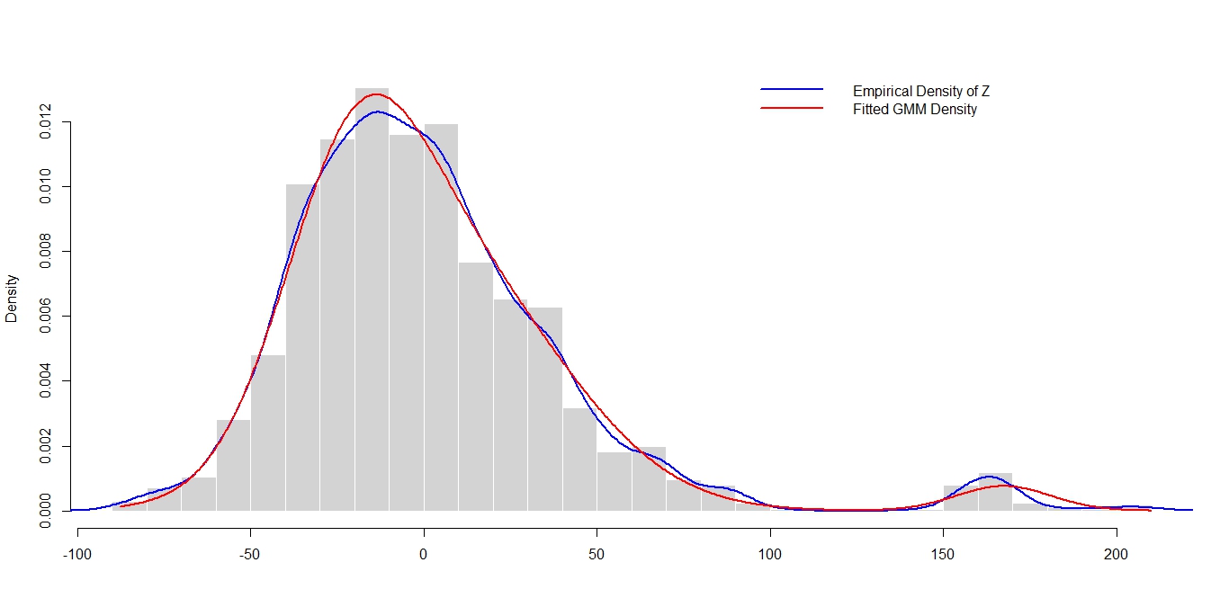
Table 5 shows that all three models identify positive effects of age, education, job class, and health on wages, with consistent coefficient signs across modelling approaches. While the estimated effects are broadly similar, differences in coefficient magnitudes are observed across the models, particularly for the health variable. These differences may be associated with the different modelling assumptions underlying the classical linear, log-linear, and copula-based approaches, including the ability of the copula model to accommodate heteroscedasticity and more flexible dependence structures. The estimated standard errors are generally small relative to the corresponding coefficient estimates, indicating reasonable estimation precision.
| Coefficients | MLR (wage scale) | Log‑linear (log scale) | Copula (wage scale) | |||
|---|---|---|---|---|---|---|
| Estimate | SE | Estimate | SE | Estimate | SE | |
| Intercept | 20.015 | 4.991 | 3.845 | 0.041 | 25.447 | 3.041 |
| Age | 0.637 | 0.068 | 0.006 | 0.001 | 0.812 | 0.067 |
| Education | 14.461 | 0.684 | 0.121 | 0.006 | 10.852 | 0.668 |
| Jobclass | 3.608 | 1.655 | 0.027 | 0.014 | 1.704 | 1.213 |
| Health | 9.245 | 1.819 | 0.086 | 0.015 | 2.375 | 1.468 |
The copula model yields the lowest training MAPE (0.28), indicating a better fit to the training data than the classical linear (0.34) and log-linear (0.34) models. Table 6 summarises the testing dataset results and shows that the copula-based regression model achieves better predictive performance compared with both the classical linear and log-linear models. The copula model produces the lowest MAE and MAPE values, while its RMSE is comparable to that of the log-linear model. Although the log-linear model improves upon the classical linear regression model, the copula-based approach further reduces the overall prediction error.
| Model | MAE | RMSE | MAPE |
|---|---|---|---|
| MLR | 30.32 | 43.97 | 0.40 |
| Log-linear | 24.47 | 35.39 | 0.36 |
| Copula | 24.45 | 35.49 | 0.26 |
These findings suggest that explicitly modelling complex dependence structures and heteroscedasticity through the copula framework can improve predictive performance. Overall, the results indicate that the copula-based regression model provides a flexible alternative to classical and log-transformed regression approaches for modelling data with non-constant variance and complex dependence structures.
5 Conclusion
This study addresses the limitations of classical regression approaches for modelling relationships in the presence of heteroscedasticity. Classical linear regression assumes constant error variance, while log-linear regression attempts to stabilise the variance through a logarithmic transformation. However, these approaches often fail when the error variance changes systematically with the predictors or when the dependence structure between variables is non-linear, asymmetric, or exhibits tail dependence. These limitations can reduce predictive accuracy and motivate the need for more flexible modelling approaches.
To overcome these challenges, this study proposed a copula-based regression framework that models the joint distribution of the response and explanatory variables through copula functions, enabling flexible modelling of non-linear, asymmetric, and tail-dependent relationships. The simulation results from both Simulation Studies I and II demonstrate that the proposed copula-based model consistently provides the best predictive performance across the considered two Scenarios, with its advantages being particularly evident under strong dependence and pronounced heteroscedasticity. The classical linear regression model generally performed better than the log-linear model, suggesting that the log-transformation did not consistently improve predictive performance under the simulated heteroscedastic settings.
In contrast, the real data application using the ISLR Wage R dataset presents a different scenario. The proposed copula-based regression framework achieved the highest predictive accuracy and the lowest prediction errors among the models considered, while the log-linear model outperformed the classical linear regression model. The improved performance of the log-linear model is likely attributable to the logarithmic transformation, which reduced the skewness of the response variable and produced a distribution that more closely approximated normality. These findings suggest that the effectiveness of log-transformations depends on the underlying data-generating process. While they can improve model performance when the response exhibits non-normality or skewness, they may be less effective in the presence of more complex heteroscedastic variance structures. Under these conditions, the proposed copula-based regression framework provides a flexible modelling approach by explicitly capturing the dependence structure and accommodating non-constant error variance.
From a methodological perspective, this study contributes by integrating heteroscedastic modelling within a copula-based regression framework and providing a systematic comparison with widely used alternatives. From a practical standpoint, the results highlight the importance of moving beyond standard transformations and adopting more flexible approaches when dealing with complex data structures. Although the proposed framework is developed using relatively parsimonious model specifications, it demonstrates consistent performance across different simulation scenarios and empirical applications.
Building on this work, future research can extend the proposed copula-based regression framework to discrete response settings, particularly count data applications. Copula-based approaches provide a flexible mechanism for modelling dependence while accommodating different marginal distributions. Beyond the classical Poisson and negative binomial models, recent developments have introduced more flexible distributions for handling both underdispersed and overdispersed count data, highlighting the need for more adaptable count-data methodologies (Doukhan et al., 2017; Safari-Katesari et al., 2020; Baker, 2026). Integrating these count-data models within the proposed copula-based framework, while accounting for heteroscedasticity and dispersion, represents a promising direction for future research and would further broaden the applicability of the framework to real-world count data (Pang, 2022).
Overall, the findings suggest that copula-based regression provides a robust and flexible alternative to classical and log-transformed regression models, providing a flexible alternative for modelling heteroscedastic data with complex dependence structures.
References
- New mixture distributions for modelling count data. Statistical Modelling 26 (3), pp. 229–247. External Links: Document Cited by: §5.
- High-dimensional gaussian copula regression: adaptive estimation and statistical inference. Statistica Sinica 31, pp. 963–993. Cited by: §1, §1.
- Multivariate count autoregression. Annals of the Institute of Statistical Mathematics 69, pp. 105–130. External Links: Document Cited by: §5.
- The logged dependent variable, heteroscedasticity, and the retransformation problem. Journal of Health Economics 17 (3), pp. 283–295. Cited by: §1, §1.
- Copula-based regression models: a survey. Journal of Statistical Planning and Inference 139 (11), pp. 3847–3856. External Links: Document Cited by: §1, §1, §1, §2.2.
- Investigation of correlated internet and smartphone addiction in adolescents: copula regression analysis. International Journal of Environmental Research and Public Health 17 (16), pp. 5806. External Links: Document Cited by: §1.
- Nonparametric estimation of multivariate copula using empirical bayes methods. Mathematics 11 (4), pp. 1234–1249. Cited by: §1.
- Estimating log models: to transform or not to transform?. Journal of Health Economics 20 (4), pp. 461–494. External Links: Document Cited by: §1.
- Investigating heteroscedasticity using the over-dispersion parameter in a travel cost model. Letters in Spatial and Resource Sciences 15 (3), pp. 507–516. External Links: Document Cited by: §5.
- Copula regression. Variance 5 (1), pp. 45–54. Cited by: §1, §1, §1.
- Generalized additive models for location, scale and shape: a distributional regression approach. Statistical Modelling 20 (3), pp. 189–211. Cited by: §1.
- Modeling count data via copulas. arXiv preprint arXiv:2012.02021. External Links: 2012.02021 Cited by: §5.
- Flexible regression and smoothing: using gamlss in r. CRC Press, Boca Raton, FL. Cited by: §1.
- Some observations on copula regression functions. Communications in Statistics – Theory and Methods 34 (9–10), pp. 1967–1978. Cited by: §2.2.
- On multivariate asymmetric dependence using multivariate skew-normal copula-based regression. International Journal of Approximate Reasoning 92, pp. 376–391. External Links: Document Cited by: §1, §1.
- Introductory econometrics: a modern approach. 7 edition, Cengage Learning. External Links: ISBN 978-1-337-55886-0 Cited by: §1, §1, §1.
Appendix A Appendix
A.1 Prediction Results for Simulation Study I


Appendix B Appendix
B.1 Prediction Results for Simulation Study II


Appendix C Appendix
C.1 Prediction Results for Negative X
| Scenario | Sample Size | Case | Mean MAPE for Each Model(with standard deviation) | ||
|---|---|---|---|---|---|
| Copula | Linear | Log-Linear | |||
| Gumble | 30 | 1 | 4.74 (0.53) | 7.35 (0.55) | 10.3 (0.88) |
| 2 | 4.69 (0.55) | 7.34 (0.58) | 9.51 (0.98) | ||
| 3 | 1.85 (0.22) | 2.51 (0.48) | 4.80 (0.60) | ||
| 50 | 1 | 4.59 (0.40) | 7.25 (0.41) | 9.33 (0.92) | |
| 2 | 4.67 (0.39) | 7.35 (0.44) | 8.57 (0.83) | ||
| 3 | 1.82 (0.17) | 2.50 (0.37) | 4.12 (0.49) | ||
| 100 | 1 | 4.51 (0.30) | 7.21 (0.32) | 8.25 (0.94) | |
| 2 | 4.59 (0.28) | 7.29 (0.33) | 7.67 (1.24) | ||
| 3 | 1.80 (0.13) | 2.49 (0.29) | 3.56 (0.43) | ||
