\hypersetup

pdftitle=A Coulomb Particle Model for Learning Kernel Attention in Transformers, pdfauthor=Masoud Badiei Khuzani, Atiq Islam, Alex Cozzi, Abraham Bagherjeiran, hypertexnames=false \hldauthor\NameMasoud Badiei Khuzani \Emailmbadieikhuzani@ebay.com
\addreBay Inc., San Jose, CA, USA and \NameSharath Honnaiah \Emailshonnaiah@ebay.com
\addreBay Inc., San Jose, CA, USA and \NameAtiq Islam \Emailatislam@ebay.com
\addreBay Inc., San Jose, CA, USA and \NameAlex Cozzi \Emailacozzi@ebay.com
\addreBay Inc., San Jose, CA, USA and \NameAbraham Bagherjeiran \Emailabagherjeiran@ebay.com
\addreBay Inc., San Jose, CA, USA

A Coulomb Particle Model for Learning Kernel Attention in Transformers

Abstract

Randomized features provide a scalable approximation to kernel machines, but their performance depends strongly on the choice of feature distribution. We propose a particle-based method that learns this distribution by optimizing kernel-target alignment while regularizing particles with a Riesz/Coulomb repulsive potential. The resulting Hamiltonian yields diverse, task-adaptive random features and admits a mean-field description through a McKean–Vlasov equation. We instantiate the method in linearized Transformer attention by learning positive random-feature maps in a first alignment phase, then freezing the kernel and training the remaining network parameters with cross-entropy. Experiments on synthetic classification and sentence-level benchmarks show that learned kernelized attention can improve accuracy, calibration, and robustness for several feature maps while preserving linear-attention inference complexity.

1 Introduction

Kernel methods are a principled way to encode nonlinear similarity, but classical training and prediction can scale poorly with the number of samples. Random Fourier features alleviate this problem by replacing an implicit kernel with an explicit randomized map (Rahimi and Recht, 2007). Nevertheless, the kernel and its associated feature distribution are typically fixed before any labels are observed—a choice that can dominate downstream performance when the appropriate similarity structure is unknown.

We study a supervised kernel-learning procedure that keeps the computational advantages of random features while learning the feature distribution from labels. The key idea is to view the random features as interacting particles. A target-alignment objective attracts particles toward features that explain the labels, while a Riesz/Coulomb repulsive energy prevents collapse and encourages diversity. This gives a concrete optimization algorithm, a statistical-mechanics interpretation, and a direct route to kernelized attention in Transformers.

Our contributions are: (i) a particle Hamiltonian for target-aligned random-feature learning; (ii) a Langevin optimization procedure with a mean-field continuum limit; (iii) an instantiation for positive random-feature attention that preserves linear-time inference; and (iv) empirical evidence that the learned kernels improve several accuracy and calibration metrics on synthetic and NLP benchmarks. Full related work, proofs, and additional ablations are in the supplementary material.

2 Particle kernel learning

Let $\phi:\mathcal{X}\times\Omega\to[-1,1]$ be a random feature map and let $\mu$ be a probability measure over feature parameters. The induced kernel is

\displaystyle K_{\mu}(\bm{x},\bm{x}^{\prime})=\mathbb{E}_{\bm{\omega}\sim\mu}[\phi_{\bm{\omega}}(\bm{x})\phi_{\bm{\omega}}(\bm{x}^{\prime})].

(2.1)

Given training data $\{(\bm{x}_{i},y_{i})\}_{i=1}^{n}$ , we learn $\mu$ by maximizing kernel-target alignment (Cristianini et al., 2002). With particles $\bm{\Omega}_{N}=(\bm{\omega}_{1},\ldots,\bm{\omega}_{N})$ and empirical measure $\mu_{N}=N^{-1}\sum_{k=1}^{N}\delta_{\bm{\omega}_{k}}$ , this becomes the finite-dimensional Hamiltonian

\displaystyle\mathcal{H}_{N}(\bm{\Omega}_{N})=-\frac{1}{n(n-1)}\sum_{i\neq j}y_{i}y_{j}\frac{1}{N}\sum_{k=1}^{N}\phi_{\bm{\omega}_{k}}(\bm{x}_{i})\phi_{\bm{\omega}_{k}}(\bm{x}_{j})+\lambda\mathcal{W}_{N,s}(\bm{\Omega}_{N}),

(2.2)

where

\displaystyle\mathcal{W}_{N,s}(\bm{\Omega}_{N})=\frac{1}{2N(N-1)}\sum_{k\neq\ell}g_{s}(\bm{\omega}_{k}-\bm{\omega}_{\ell}),\qquad g_{s}(\bm{\omega})=\begin{cases}\|\bm{\omega}\|_{2}^{-s},&s>0,\\ -\log\|\bm{\omega}\|_{2},&s=0.\end{cases}

(2.3)

The first term rewards features whose empirical kernel aligns with labels; the second term spreads particles across $\Omega$ . For random Fourier features, this energy reduces to a trigonometric alignment objective involving $\cos(\bm{X}\bm{\Omega}_{N}^{\top})$ and $\sin(\bm{X}\bm{\Omega}_{N}^{\top})$ , which makes the objective differentiable and easy to optimize.

{algorithm2e}

[!t] Projected Langevin feature learning \DontPrintSemicolon\KwDataparticles $\{\bm{\omega}_{k}^{0}\}_{k=1}^{N}$ , step $\eta$ , inverse temperature $\beta$ , threshold $\delta$ \KwResultlearned empirical feature law $\mu_{N}$ and kernel $\widehat{K}$ Initialize $\mu_{N}^{0}=N^{-1}\sum_{k}\delta_{\bm{\omega}_{k}^{0}}$ \Repeat $\mathcal{D}(\mu_{N}^{m},\mu_{N}^{m-1})<\delta$ \For $k=1,\ldots,N$ Draw $\bm{\xi}_{k}^{m}\sim\mathcal{N}(0,I)$ and set $\bm{\omega}_{k}^{m+1}=\mathcal{P}_{\Omega}(\bm{\omega}_{k}^{m}-\eta N\nabla_{\bm{\omega}_{k}}\mathcal{H}_{N}(\bm{\Omega}_{N}^{m})+\sqrt{2\eta/\beta}\,\bm{\xi}_{k}^{m})$ $\mu_{N}^{m+1}=N^{-1}\sum_{k}\delta_{\bm{\omega}_{k}^{m+1}}$ Return $\widehat{K}(\bm{x},\bm{x}^{\prime})=D^{-1}\sum_{k=1}^{D}\phi_{\bm{\omega}_{k}}(\bm{x})\phi_{\bm{\omega}_{k}}(\bm{x}^{\prime})$

3 Kernelized attention

Self-attention can be written as a normalized kernel smoother (Vaswani et al., 2017; Nadaraya, 1964; Watson, 1964):

\displaystyle\bm{a}_{i}(\bm{X})=\frac{\sum_{j=0}^{\ell}K(\bm{q}_{i},\bm{k}_{j})\bm{v}_{j}}{\sum_{j=0}^{\ell}K(\bm{q}_{i},\bm{k}_{j})},\qquad K(\bm{q},\bm{k})=\exp(\bm{q}^{\top}\bm{k}/\sqrt{d}).

(3.1)

Replacing $K$ by a positive random-feature kernel $K_{\bm{\Omega}_{N}}(\bm{q},\bm{k})=\bm{\phi}_{\bm{\Omega}_{N}}(\bm{q})^{\top}\bm{\phi}_{\bm{\Omega}_{N}}(\bm{k})$ gives the linearized attention estimator

\displaystyle\widehat{\bm{a}}_{i}(\bm{X})=\frac{\bm{\phi}_{\bm{\Omega}_{N}}(\bm{q}_{i})^{\top}\big(\sum_{j}\bm{\phi}_{\bm{\Omega}_{N}}(\bm{k}_{j})\bm{v}_{j}^{\top}\big)}{\bm{\phi}_{\bm{\Omega}_{N}}(\bm{q}_{i})^{\top}\big(\sum_{j}\bm{\phi}_{\bm{\Omega}_{N}}(\bm{k}_{j})\big)}.

(3.2)

This preserves the normalized kernel-smoothing form but reduces the per-head sequence-length dependence from quadratic to linear in $\ell$ , up to the feature dimension (Katharopoulos et al., 2020a; Choromanski et al., 2021; Peng et al., 2021). In Phase A, we learn the feature particles $\bm{\Omega}_{N}$ by alignment on sequence representations. In Phase B, we freeze $\bm{\Omega}_{N}$ and train the remaining Transformer parameters using cross-entropy.

4 Theoretical results: mean-field limit and large deviation principle

The particle view gives both a continuum training dynamics and an equilibrium concentration result. Define the alignment-induced potential

\displaystyle V_{\mathcal{D}}(\bm{\omega})=-\frac{1}{n(n-1)}\sum_{i\neq j}y_{i}y_{j}\phi_{\bm{\omega}}(\bm{x}_{i})\phi_{\bm{\omega}}(\bm{x}_{j}),

(4.1)

and the continuum energy

\displaystyle\mathcal{E}_{s}(\mu)=\int V_{\mathcal{D}}(\bm{\omega})\,d\mu(\bm{\omega})+\frac{\lambda}{2}\iint g_{s}(\bm{\omega}-\bm{\omega}^{\prime})\,d\mu(\bm{\omega})d\mu(\bm{\omega}^{\prime}).

(4.2)

The finite-particle optimizer has the following continuum training law.

Theorem 4.1 (Projected-particle McKean–Vlasov mean-field limit).

Let $\Omega\subset\mathbb{R}^{d}$ be compact and convex with $C^{2}$ boundary and outward normal $\bm{n}$ . Assume $V_{\mathcal{D}}\in C^{2}(\overline{\Omega})$ , a Lipschitz regularized interaction drift, exchangeable $\mu_{0}^{N}\Rightarrow\rho_{0}d\bm{\omega}$ , and a vanishing projected-Euler error. If

\displaystyle\bm{\omega}_{k}^{m+1}=\mathcal{P}_{\overline{\Omega}}\!\left(\bm{\omega}_{k}^{m}-\eta_{N}N\nabla_{\bm{\omega}_{k}}\mathcal{H}_{N}(\bm{\Omega}_{N}^{m})+\sqrt{2\eta_{N}/\beta}\,\bm{\xi}_{k}^{m}\right),\quad\eta_{N}\downarrow 0,

(4.3)

then $\mu_{t}^{N}=N^{-1}\sum_{k}\delta_{\bm{\omega}_{k}^{\lfloor t/\eta_{N}\rfloor}}\Rightarrow\rho_{t}d\bm{\omega}$ in probability, uniformly on compact time intervals. With $U_{t}=V_{\mathcal{D}}+\lambda g_{s}\ast\rho_{t}$ ,

	$\displaystyle\partial_{t}\rho_{t}=\nabla\!\cdot(\rho_{t}\nabla U_{t})+\beta^{-1}\Delta\rho_{t},$		(4.4)
	$\displaystyle\rho_{t}\|_{t=0}=\rho_{0},\qquad(\rho_{t}\nabla U_{t}+\beta^{-1}\nabla\rho_{t})\!\cdot\bm{n}=0\quad\text{on }\partial\Omega,$		(4.5)

equivalently $\partial_{\bm{n}}\rho_{t}+\beta\rho_{t}\partial_{\bm{n}}U_{t}=0$ . Moreover $\rho_{t}\geq 0$ and $\int_{\Omega}\rho_{t}=1$ .

The proof is provided in the supplementary material. The two parts of $U_{t}$ have distinct roles. The data potential $V_{\mathcal{D}}$ pulls mass toward features that reduce the empirical objective, while the interaction term spreads mass according to the regularized Riesz geometry and prevents all features from collapsing onto the same locations. The diffusion term $\beta^{-1}\Delta\rho_{t}$ is the continuum trace of the Langevin noise: at finite temperature it encourages exploration and contributes an entropic regularization; in the zero-temperature limit the equation reduces to the deterministic transport law driven by $-\nabla U_{t}$ . Equivalently,

\displaystyle\partial_{t}\rho_{t}=\nabla\!\cdot\left(\rho_{t}\nabla\left(U_{t}+\beta^{-1}\log\rho_{t}\right)\right),

so (4.5) is the Wasserstein gradient flow of $\mathcal{F}_{\beta}(\rho)\stackrel{{\scriptstyle\mathrm{def}}}{{=}}\mathcal{E}_{s}(\rho)+\beta^{-1}\operatorname{Ent}(\rho\mid\ell).$ For smooth positive solutions the no-flux condition removes the boundary contribution and gives the dissipation identity

\displaystyle\frac{d}{dt}\mathcal{F}_{\beta}(\rho_{t})=-\int_{\Omega}\rho_{t}\left|\nabla\left(U_{t}+\beta^{-1}\log\rho_{t}\right)\right|^{2}d\bm{\omega}\leq 0.

This identity is useful conceptually: training decreases the continuum free energy, and the only stationary points are self-consistent Gibbs densities of the form

\displaystyle\rho_{\infty}(\bm{\omega})=\frac{1}{Z_{\infty}}\exp\{-\beta[V_{\mathcal{D}}(\bm{\omega})+\lambda(g_{s}\ast\rho_{\infty})(\bm{\omega})]\},

with the boundary condition inherited from projection.

Theorem 4.2 (Large deviations for learned feature measures).

Let $\Omega\subset\mathbb{R}^{d}$ be bounded and let $s>d$ . If $\bm{\Omega}_{N}\sim\prob_{N,\beta_N}$ and $\mu_{N}=N^{-1}\sum_{k=1}^{N}\delta_{\bm{\omega}_{k}}$, then $\{\mu_{N}\}$ satisfies an LDP on $\mathcal{P}(\Omega)$. When $\beta_{N}/N\to 1$, the speed is $r_{N}=N$ and \@@amsalign\mathcal{J}_{s}(\mu)=\mathcal{E}_{s}(\mu)+\operatorname{Ent}(\mu\mid\ell)-\inf_{\nu}\{\mathcal{E}_{s}(\nu)+\operatorname{Ent}(\nu\mid\ell)\}, where $\operatorname{Ent}(\mu\mid\ell)=\int\log(d\mu/d\ell)d\mu$ for $\mu\ll\ell$. When $\beta_{N}/N\to\infty$, the speed is $r_{N}=\beta_{N}$ and \@@amsalign\mathcal{J}_{s}(\mu)=\mathcal{E}_{s}(\mu)-\inf_{\nu}\mathcal{E}_{s}(\nu). For Borel $A\subset\mathcal{P}(\Omega)$, the standard LDP hold with rate $\mathcal{J}_{s}$ and speed $r_{N}$. \end{theorem}ThesupplementprovesthisbycombiningSanov^{\prime}stheoremwithVaradhan^{\prime}slemmaaftertruncatingthesingularRieszinteraction.Consequentlythelearnedkernelconcentratesaroundthetask-adaptivevariationalkernel;iftherelevantratehasauniqueminimizer$\mu_{s}^{\star}$,then$K_{\mu_{N}}(\bm{x},\bm{x}^{\prime})\to K_{\mu_{s}^{\star}}(\bm{x},\bm{x}^{\prime})$exponentiallyatspeed$N$or$\beta_{N}$.\par$

5 Experiments

We evaluate on synthetic classification and SST-2, QQP, and Rotten Tomatoes. Synthetic results show that optimized particles outperform fixed random Fourier features and the importance-sampling baseline under moderate noise. The accuracy gap widens with feature budget: at 64 features per head, optimized particles retain roughly 90% of the performance achieved at 256, while fixed random features degrade more sharply. NLP experiments use a two-layer Transformer encoder with hidden size 128, two heads, 256 random features per head, BERT tokenization, batch size 64, and the two-phase alignment-then-cross-entropy protocol. Training uses AdamW with linear warmup and cosine decay; the alignment phase runs for 20% of total steps before switching to cross-entropy fine-tuning. All results are averaged over three random seeds.

We report the full detailed result tables for the three text-classification tasks in the main paper. For all rows in the lower block of each table, the attention projection is constrained to $Q=K=\mathrm{reshape}(x)$ , so vanilla and learned-kernel rows are matched feature-map comparisons. The reported metrics include accuracy, micro/macro/weighted F1, ROC-AUC, PR-AUC, MCC, balanced accuracy, LogLoss, Brier score, ECE, and wall-clock training time.

Table 1: SST-2 detailed metrics across attention variants. Bold marks the best value per column; lower is better for LogLoss, Brier, ECE, and train time.

Learned $W_{q},W_{k}$ baselines
Model	Acc $\uparrow$	F1 $\bm{\mu}\uparrow$	F1M $\uparrow$	F1w $\uparrow$	ROC-AUC $\uparrow$	PR-AUC $\uparrow$	MCC $\uparrow$	BalAcc $\uparrow$	LogLoss $\downarrow$	Brier $\downarrow$	ECE $\downarrow$	Train(sec) $\downarrow$
Vaswani-softmaxattn	0.8050	0.8050	0.8050	0.8051	0.8744	0.8856	0.6100	0.8050	0.5083	0.1498	0.3695	86.8
Vanilla-favor-WqWk	0.7833	0.7833	0.7832	0.7832	0.8587	0.8576	0.5676	0.7837	0.5472	0.1592	0.3584	96.5
Performer	0.7798	0.7798	0.7793	0.7791	0.8618	0.8766	0.5656	0.7810	0.5697	0.1666	0.3804	89.0
Linformer	0.7844	0.7844	0.7843	0.7843	0.8569	0.8673	0.5706	0.7850	0.5922	0.1646	0.3782	82.6
No learned $W_{q},W_{k}$ (Q=K=reshape(x)); feature-map variants
Vanilla-favor	0.8050	0.8050	0.8050	0.8049	0.8841	0.8928	0.6124	0.8057	0.4362	0.1388	0.3420	80.5
Kernel-favor	0.7901	0.7901	0.7900	0.7901	0.8734	0.8834	0.5801	0.7899	0.4477	0.1459	0.3086	166.0
Vanilla-elu	0.8028	0.8028	0.8019	0.8017	0.8731	0.8803	0.6150	0.8042	0.4938	0.1505	0.3724	78.8
Kernel-elu	0.8108	0.8108	0.8107	0.8108	0.8879	0.8913	0.6216	0.8108	0.4502	0.1392	0.3609	164.3
Vanilla-softplus	0.8108	0.8108	0.8108	0.8108	0.8760	0.8837	0.6225	0.8112	0.4582	0.1429	0.3378	88.5
Kernel-softplus	0.8062	0.8062	0.8058	0.8060	0.8861	0.8864	0.6126	0.8057	0.5122	0.1470	0.3920	173.5
Vanilla-sigmoid2	0.7959	0.7959	0.7957	0.7958	0.8786	0.8881	0.5916	0.7956	0.5025	0.1487	0.3744	82.6
Kernel-sigmoid2	0.7924	0.7924	0.7924	0.7924	0.8785	0.8880	0.5863	0.7929	0.4915	0.1516	0.3790	170.1
Vanilla-softmaxfeat	0.8005	0.8005	0.8003	0.8004	0.8683	0.8728	0.6008	0.8001	0.5163	0.1530	0.3621	89.5
Kernel-softmaxfeat	0.8085	0.8085	0.8085	0.8084	0.8858	0.8982	0.6181	0.8089	0.4381	0.1389	0.3526	171.4
Vanilla-cos2	0.8142	0.8142	0.8142	0.8141	0.8897	0.8945	0.6305	0.8148	0.4709	0.1395	0.3866	81.5
Kernel-cos2	0.8119	0.8119	0.8118	0.8119	0.8883	0.8976	0.6237	0.8118	0.4422	0.1366	0.3557	165.0
Vanilla-porf-softplus	0.8142	0.8142	0.8142	0.8142	0.8883	0.8983	0.6285	0.8143	0.4506	0.1380	0.3569	85.7
Kernel-porf-softplus	0.8188	0.8188	0.8188	0.8188	0.8897	0.8967	0.6376	0.8189	0.4561	0.1381	0.3734	162.8

Table 2: QQP detailed metrics across attention variants. Bold marks the best value per column; lower is better for LogLoss, Brier, ECE, and train time.

Learned $W_{q},W_{k}$ baselines
Model	Acc $\uparrow$	F1 $\bm{\mu}\uparrow$	F1M $\uparrow$	F1w $\uparrow$	ROC-AUC $\uparrow$	PR-AUC $\uparrow$	MCC $\uparrow$	BalAcc $\uparrow$	LogLoss $\downarrow$	Brier $\downarrow$	ECE $\downarrow$	Train(sec) $\downarrow$
Vaswani-softmaxattn	0.8005	0.8005	0.7949	0.8038	0.8959	0.8266	0.6058	0.8133	0.4112	0.1350	0.4314	605.9
Vanilla-favor-WqWk	0.7683	0.7683	0.7346	0.7595	0.8313	0.7619	0.4852	0.7248	0.4863	0.1591	0.4383	539.7
Performer	0.7751	0.7751	0.7472	0.7693	0.8402	0.7691	0.5030	0.7388	0.4732	0.1547	0.4360	554.1
Linformer	0.8077	0.8077	0.7944	0.8082	0.8828	0.8157	0.5890	0.7960	0.4153	0.1337	0.4541	557.1
No learned $W_{q},W_{k}$ (Q=K=reshape(x)); feature-map variants
Vanilla-favor	0.7626	0.7626	0.7323	0.7560	0.8168	0.7443	0.4741	0.7242	0.5028	0.1637	0.4182	567.8
Kernel-favor	0.7608	0.7608	0.7319	0.7551	0.8158	0.7438	0.4712	0.7246	0.5016	0.1638	0.4106	1197.1
Vanilla-elu	0.7797	0.7797	0.7553	0.7757	0.8458	0.7772	0.5155	0.7485	0.4659	0.1518	0.4386	585.1
Kernel-elu	0.7831	0.7831	0.7648	0.7821	0.8533	0.7863	0.5299	0.7625	0.4598	0.1496	0.4474	1110.3
Vanilla-softplus	0.7786	0.7786	0.7522	0.7735	0.8442	0.7747	0.5116	0.7444	0.4656	0.1522	0.4297	633.3
Kernel-softplus	0.7860	0.7860	0.7651	0.7836	0.8564	0.7891	0.5323	0.7603	0.4578	0.1481	0.4582	1100.7
Vanilla-sigmoid2	0.7772	0.7772	0.7580	0.7760	0.8439	0.7728	0.5165	0.7554	0.4664	0.1529	0.4190	591.9
Kernel-sigmoid2	0.7852	0.7852	0.7666	0.7840	0.8549	0.7885	0.5338	0.7639	0.4537	0.1479	0.4415	1156.0
Vanilla-softmaxfeat	0.7801	0.7801	0.7527	0.7744	0.8471	0.7772	0.5143	0.7441	0.4625	0.1512	0.4365	579.9
Kernel-softmaxfeat	0.7909	0.7909	0.7753	0.7909	0.8679	0.7956	0.5506	0.7753	0.4354	0.1418	0.4371	1072.6
Vanilla-cos2	0.7746	0.7746	0.7533	0.7724	0.8422	0.7715	0.5082	0.7492	0.4688	0.1536	0.4249	650.2
Kernel-cos2	0.7842	0.7842	0.7590	0.7795	0.8525	0.7842	0.5245	0.7511	0.4621	0.1497	0.4526	1254.0
Vanilla-porf_softplus	0.7782	0.7782	0.7531	0.7739	0.8434	0.7751	0.5117	0.7461	0.4685	0.1528	0.4401	588.4
Kernel-porf_softplus	0.7841	0.7841	0.7632	0.7817	0.8536	0.7855	0.5284	0.7585	0.4547	0.1483	0.4419	1110.4

Table 3: Rotten Tomatoes detailed metrics across attention variants. Bold marks the best value per column; lower is better for LogLoss, Brier, ECE, and train time.

Learned $W_{q},W_{k}$ baselines
Model	Acc $\uparrow$	F1 $\bm{\mu}\uparrow$	F1M $\uparrow$	F1w $\uparrow$	ROC-AUC $\uparrow$	PR-AUC $\uparrow$	MCC $\uparrow$	BalAcc $\uparrow$	LogLoss $\downarrow$	Brier $\downarrow$	ECE $\downarrow$	Train(sec) $\downarrow$
Vaswani-softmaxattn	0.6801	0.6801	0.6793	0.6793	0.7492	0.7522	0.3620	0.6801	0.6396	0.2138	0.2751	12.6
Vanilla-favor-WqWk	0.6764	0.6764	0.6758	0.6758	0.7262	0.7162	0.3539	0.6764	0.7265	0.2327	0.3052	13.0
Performer	0.6642	0.6642	0.6616	0.6616	0.7262	0.7075	0.3333	0.6642	0.7477	0.2347	0.3009	14.4
Linformer	0.6614	0.6614	0.6612	0.6612	0.7133	0.7062	0.3230	0.6614	0.6614	0.2260	0.2509	13.7
No learned $W_{q},W_{k}$ (Q=K=reshape(x)); feature-map variants
Vanilla-favor	0.7083	0.7083	0.7066	0.7066	0.7732	0.7708	0.4214	0.7083	0.5840	0.1977	0.2229	13.7
Kernel-favor	0.6848	0.6848	0.6848	0.6848	0.7597	0.7479	0.3696	0.6848	0.5823	0.1997	0.2193	26.3
Vanilla-elu	0.6895	0.6895	0.6835	0.6835	0.7844	0.7928	0.3943	0.6895	0.5809	0.1995	0.2435	12.7
Kernel-elu	0.7148	0.7148	0.7140	0.7140	0.7650	0.7586	0.4320	0.7148	0.5860	0.1991	0.2594	26.1
Vanilla-softplus	0.7036	0.7036	0.7023	0.7023	0.7695	0.7580	0.4107	0.7036	0.5838	0.1977	0.2176	12.6
Kernel-softplus	0.7017	0.7017	0.7017	0.7017	0.7743	0.7677	0.4034	0.7017	0.5766	0.1959	0.2517	23.8
Vanilla-sigmoid2	0.7026	0.7026	0.7022	0.7022	0.7714	0.7675	0.4065	0.7026	0.5758	0.1958	0.2408	12.7
Kernel-sigmoid2	0.6876	0.6876	0.6831	0.6831	0.7562	0.7538	0.3864	0.6876	0.6118	0.2091	0.2733	24.0
Vanilla-softmaxfeat	0.6782	0.6782	0.6733	0.6733	0.7664	0.7703	0.3678	0.6782	0.6065	0.2071	0.2610	12.5
Kernel-softmaxfeat	0.7167	0.7167	0.7163	0.7163	0.7779	0.7724	0.4345	0.7167	0.5697	0.1929	0.2527	24.5
Vanilla-cos2	0.6876	0.6876	0.6855	0.6855	0.7622	0.7586	0.3803	0.6876	0.5897	0.2015	0.2154	12.4
Kernel-cos2	0.7092	0.7092	0.7091	0.7091	0.7676	0.7680	0.4185	0.7092	0.5836	0.1982	0.2594	26.7
Vanilla-porf_softplus	0.6839	0.6839	0.6832	0.6832	0.7649	0.7637	0.3692	0.6839	0.5858	0.1996	0.2343	12.6
Kernel-porf_softplus	0.6989	0.6989	0.6986	0.6986	0.7702	0.7700	0.3984	0.6989	0.5750	0.1961	0.2378	24.1

Tables 1, 2, and 3 show that kernel learning is feature-map dependent but often improves both discrimination and proper scoring metrics. On SST-2, Kernel-PORF-softplus gives the highest accuracy and MCC, while Kernel-FAVOR gives the lowest ECE. On QQP, Kernel-softmaxfeat is the strongest $Q=K$ model and reduces LogLoss and Brier score relative to its vanilla counterpart. On Rotten Tomatoes, Kernel-softmaxfeat gives the best accuracy, MCC, LogLoss, and Brier score. The training-time column reflects the one-time alignment phase; after particles are learned, the serving-time attention formula remains linear in sequence length.

Additional experiment details.

Inputs use the bert-base-uncased WordPiece tokenizer, are padded or truncated to 128 tokens, and use mean pooling over final token representations. The Transformer has two encoder layers, hidden size 128, two attention heads, feed-forward dimension 256, dropout 0.1, and 256 random features per head. Phase A optimizes only the feature particles $\bm{\Omega}_{N}$ using the alignment objective with Langevin noise, log-repulsion, norm projection, and early stopping; Phase B freezes the learned particles and trains the remaining classifier with cross-entropy. Thus the extra cost appears during training, while inference uses the same linear-attention structure as the corresponding vanilla feature map.

6 Conclusion

We introduced a Coulomb/Riesz particle model for supervised random-feature learning and applied it to kernelized Transformer attention. The framework links label alignment, repulsive regularization, Langevin optimization, and equilibrium concentration in a single formulation. Empirically, the method improves several random-feature attention variants and provides a practical way to learn task-adaptive linear-attention kernels.

LLM usage statement.

The authors used large language model (LLM) tools for writing assistance and code development. All LLM-assisted content was reviewed, verified, and edited by the authors, who take full responsibility for the correctness, originality, citations, proofs, experiments, figures, and final content of this paper.

References

Bach et al. (2004) Francis R Bach, Gert RG Lanckriet, and Michael I Jordan. Multiple kernel learning, conic duality, and the SMO algorithm. In Proceedings of the twenty-first international conference on Machine learning, page 6, 2004.
Chapelle et al. (2002) Olivier Chapelle, Vladimir Vapnik, Olivier Bousquet, and Sayan Mukherjee. Choosing multiple parameters for support vector machines. Machine Learning, 46(1–3):131–159, 2002. 10.1023/A:1012450327387.
Chen et al. (2021) Yifan Chen, Qi Zeng, Heng Ji, and Yun Yang. Skyformer: Remodel self-attention with gaussian kernel and nyström method. In Advances in Neural Information Processing Systems, 2021.
Choromanski et al. (2017) Krzysztof Choromanski, Mark Rowland, and Adrian Weller. Structured orthogonal random features. In AISTATS, 2017.
Choromanski et al. (2020) Krzysztof Choromanski, Valerii Likhosherstov, David Dohan, Xingyou Song, Andreea Gane, Tamás Sarlós, Peter Hawkins, Jared Q. Davis, Afroz Mohiuddin, Łukasz Kaiser, David Belanger, Lucy J. Colwell, and Adrian Weller. Rethinking attention with performers. arXiv preprint arXiv:2009.14794, 2020. URL https://arxiv.org/abs/2009.14794.
Choromanski et al. (2021) Krzysztof Choromanski, Valerii Likhosherstov, David Dohan, Xingyou Song, Andreea Gane, Tam’as Sarl’os, Peter Hawkins, Jared Q. Davis, Afroz Mohiuddin, Łukasz Kaiser, David Belanger, Lucy J. Colwell, and Adrian Weller. Rethinking attention with performers. In International Conference on Learning Representations, 2021. URL https://openreview.net/forum?id=Ua6zuk0WRH.
Clevert et al. (2015) Djork-Arné Clevert, Thomas Unterthiner, and Sepp Hochreiter. Fast and accurate deep network learning by exponential linear units (elus). arXiv:1511.07289, 2015.
Cortes et al. (2009) Corinna Cortes, Mehryar Mohri, and Afshin Rostamizadeh. Learning non-linear combinations of kernels. Advances in neural information processing systems, 22, 2009.
Cortes et al. (2010) Corinna Cortes, Mehryar Mohri, and Afshin Rostamizadeh. Two-stage learning kernel algorithms. In Proceedings of the 27th International Conference on Machine Learning (ICML-10), pages 239–246, 2010.
Cristianini et al. (2002) Nello Cristianini, John Shawe-Taylor, André Elisseeff, and Jaswinder Singh Kandola. On kernel-target alignment. In Advances in neural information processing systems, volume 14, pages 367–373, 2002.
Dembo and Zeitouni (2009) Amir Dembo and Ofer Zeitouni. Large Deviations Techniques and Applications, volume 38 of Stochastic Modelling and Applied Probability. Springer, Berlin, Heidelberg, 2nd edition edition, 2009. ISBN 978-3-642-03310-0. 10.1007/978-3-642-03311-7.
Devlin et al. (2019) Jacob Devlin, Ming-Wei Chang, Kenton Lee, and Kristina Toutanova. Bert: Pre-training of deep bidirectional transformers for language understanding. In NAACL-HLT, 2019.
Dugas et al. (2001) Charles Dugas, Yoshua Bengio, François Bélisle, Claude Nadeau, and René Garcia. Incorporating second-order functional knowledge for better option pricing. In NeurIPS, 2001.
Ellis (2005) Richard S. Ellis. Entropy, Large Deviations, and Statistical Mechanics. Springer Monographs in Mathematics. Springer, June 2005. 10.1007/0-387-28537-0.
Kandola et al. (2002) Jaswinder Singh Kandola, John Shawe-Taylor, and Nello Cristianini. Optimizing kernel alignment over combinations of kernels. Technical report, University of Southampton, 2002.
Katharopoulos et al. (2020a) Angelos Katharopoulos, Apoorv Vyas, Nikolaos Pappas, and François Fleuret. Transformers are rnns: Fast autoregressive transformers with linear attention. In Proceedings of the 37th International Conference on Machine Learning (PMLR 119), 2020a.
Katharopoulos et al. (2020b) Angelos Katharopoulos, Apoorv Vyas, Nikolaos Pappas, and François Fleuret. Transformers are RNNs: Fast autoregressive transformers with linear attention. In Proceedings of the 37th International Conference on Machine Learning, volume 119 of Proceedings of Machine Learning Research, pages 5156–5165. PMLR, 2020b. URL https://proceedings.mlr.press/v119/katharopoulos20a.html.
Lanckriet et al. (2004) Gert RG Lanckriet, Nello Cristianini, Peter Bartlett, Laurent El Ghaoui, and Michael I Jordan. Learning the kernel matrix with semidefinite programming. Journal of Machine Learning Research, 5:27–72, 2004.
Lauriola and Aiolli (2020) Ivano Lauriola and Fabio Aiolli. MKLpy: a python-based framework for multiple kernel learning. arXiv preprint arXiv:2007.09982, 2020.
Luo et al. (2021) Shengjie Luo, Shanda Li, Tianle Cai, Di He, Dinglan Peng, Shuxin Zheng, Guolin Ke, Liwei Wang, and Tie-Yan Liu. Stable, fast and accurate: Kernelized attention with relative positional encoding. arXiv:2106.12566, 2021.
Micchelli and Pontil (2005) Charles A Micchelli and Massimiliano Pontil. Learning the kernel function via regularization. Journal of Machine Learning Research, 6:1099–1125, 2005.
Nadaraya (1964) E. A. Nadaraya. On estimating regression. Theory of Probability and its Applications, 1964.
Ober et al. (2021) Stefan Ober, Carl Edward Rasmussen, and Mark Van der Wilk. The promises and pitfalls of deep kernel learning. Journal of Machine Learning Research, 22(179):1–65, 2021.
Pang and Lee (2005) Bo Pang and Lillian Lee. Seeing stars: Exploiting class relationships for sentiment categorization with respect to rating scales. In Proceedings of the 43rd Annual Meeting of the Association for Computational Linguistics (ACL), pages 115–124. Association for Computational Linguistics, 2005.
Peng et al. (2021) Hao Peng, Nikolaos Pappas, Dani Yogatama, Roy Schwartz, Noah A. Smith, and Lingpeng Kong. Random feature attention. arXiv:2103.02143, 2021.
Rahimi and Recht (2009) Ali Rahimi and Ben Recht. Weighted sums of random kitchen sinks: Replacing minimization with randomization in learning. In NeurIPS, 2009.
Rahimi and Recht (2007) Ali Rahimi and Benjamin Recht. Random features for large-scale kernel machines. In Advances in Neural Information Processing Systems, volume 20, pages 1177–1184, 2007.
Rakotomamonjy et al. (2008) Alain Rakotomamonjy, Francis R Bach, St’ephane Canu, and Yves Grandvalet. SimpleMKL. Journal of Machine Learning Research, 9:2491–2521, 2008.
Sinha and Duchi (2016) Samarth Sinha and John C Duchi. Learning kernels with random features. In Advances in Neural Information Processing Systems, pages 1298–1306, 2016.
Socher et al. (2013) Richard Socher, Alex Perelygin, Jean Wu, Jason Chuang, Christopher D. Manning, Andrew Y. Ng, and Christopher Potts. Recursive deep models for semantic compositionality over a sentiment treebank. In Proceedings of the 2013 Conference on Empirical Methods in Natural Language Processing (EMNLP), pages 1631–1642, 2013.
Tsai et al. (2019) Yao-Hung Hubert Tsai, Shaojie Bai, Makoto Yamada, Louis-Philippe Morency, and Ruslan Salakhutdinov. Transformer dissection: A unified understanding of transformer’s attention via the lens of kernel. In EMNLP-IJCNLP, 2019.
Varadhan (2016) S. R. S. Varadhan. Large Deviations, volume 27 of Courant Lecture Notes. American Mathematical Society, 2016. ISBN 978-1-4704-2580-1.
Vaswani et al. (2017) Ashish Vaswani, Noam Shazeer, Niki Parmar, Jakob Uszkoreit, Llion Jones, Aidan N. Gomez, Lukasz Kaiser, and Illia Polosukhin. Attention is all you need. In Advances in Neural Information Processing Systems, 2017.
Wang et al. (2019) Alex Wang, Amanpreet Singh, Julian Michael, et al. GLUE: A multi-task benchmark and analysis platform for natural language understanding. In Proceedings of the 7th International Conference on Learning Representations (Workshop Track), 2019. URL https://openreview.net/forum?id=rJ4km2R5t7.
Watson (1964) G. S. Watson. Smooth regression analysis. Sankhyā, Series A, 1964.
Wilson et al. (2016) Andrew Gordon Wilson, Zhiting Hu, Ruslan Salakhutdinov, and Eric P Xing. Deep kernel learning. In Artificial intelligence and statistics, pages 370–378. PMLR, 2016.
Xiong et al. (2021) Yunyang Xiong, Zhanpeng Zeng, Rudrasis Chakraborty, Mingxing Tan, Glenn Fung, Yin Li, and Vikas Singh. Nyströmformer: A nyström-based algorithm for approximating self-attention. In AAAI Conference on Artificial Intelligence, 2021.
Yu et al. (2016) Felix X. Yu, Ananda Theertha Suresh, Krzysztof Choromanski, Daniel Holtmann-Rice, and Sanjiv Kumar. Orthogonal random features. In NeurIPS, 2016.

Supplementary Material

Appendix A Related work

To discuss related work, we first describe the kernel selection problem in the context of supervised learning problem. Consider a set of $n$ feature vectors and labels $\{(\bm{x}_{i},y_{i})\}_{i=1}^{n},\bm{x}_{i}\in\mathcal{X},y_{i}\in\mathcal{Y}$ . We have a loss function $L:\real\times\real\rightarrow\real$ , where $L(\cdot,y)$ is convex for $y\in\mathcal{Y}$ , and a reproducing kernel Hilbert space (RKHS) of functions $\mathcal{F}$ with kernel $K$ . The $\ell_{2}$ -regularized optimization problem that underlies the learning task of finding a function $f\in\mathcal{F}$ is as follows

\displaystyle\text{Primal:}\min_{f\in\mathcal{F}}\dfrac{1}{n}\sum_{i=1}^{n}L(f(\bm{x}_{i}),y_{i})+\dfrac{\lambda}{2}\|f\|_{\mathcal{H}}^{2},\quad\text{Dual:}\max_{\bm{\alpha}\in\mathbb{R}^{n}}-\frac{1}{n}\sum_{i=1}^{n}L^{*}(\alpha_{i},y_{i})-\frac{1}{2\lambda}\bm{\alpha}^{\top}\mathbf{K}\bm{\alpha},

(A.1)

where $\|\cdot\|_{\mathcal{H}}$ is the Hilbert space norm, $\bm{\alpha}\in\mathbb{R}^{n}$ are dual variables, $L^{*}(\alpha,y)=\sup_{z\in\mathbb{R}}\left\{\alpha z-L(z,y)\right\}$ is the Fenchel conjugate of the loss function $L$ , and $\bm{K}\stackrel{{\scriptstyle\text{def}}}{{=}}[K_{ij}]\in\real^{n\times n}$ with $K_{ij}\stackrel{{\scriptstyle\text{def}}}{{=}}K(\bm{x}_{i},\bm{x}_{j})$ is the kernel matrix.

While the kernel matrix $\mathbf{K}$ could, in principle, be optimized jointly with the dual variables, much of the literature instead focuses on approaches that decouple kernel learning from the estimation of $f\in\mathcal{F}$ . A common strategy is to first construct or adapt the kernel—often by maximizing kernel–target alignment, which quantifies the similarity between the kernel and the target—before solving the regularized risk minimization problem (see, e.g., Cortes et al. (2010); Cristianini et al. (2002); Kandola et al. (2002); Lanckriet et al. (2004)). This alignment is formulated as the following optimization problem:

\displaystyle\max_{K\in\mathcal{K}}\dfrac{1}{n(n-1)}\sum_{1\leq i\not=j\leq n}y_{i}y_{j}K(\bm{x}_{i},\bm{x}_{j}),

(A.2)

where $\mathcal{K}$ denotes a predefined class of kernel functions. Several approaches have been proposed in the literature for defining the class of kernels $\mathcal{K}$ in kernel-based learning. In Table 4, we provide a summary of common kernel class choices, along with their computational and memory complexities, as well as the corresponding references. Among the proposed approaches, Sinha and Duchi (2016) stands out as a framework that seamlessly integrates with the random feature model, specifically by employing importance sampling of random features within the random feature-based kernel class. In contrast, we propose an alternative approach that yields improved performance. This enhancement is achieved by directly optimizing the distribution of random features within a particle optimization framework, as opposed to relying on importance sampling of random features.

Table 4: Summary of kernel class

\mathcal{K}

choices in the literature. Notes.

n

: number of training samples;

m

: number of base kernels;

D

: number of random features;

d

: dimensionality of the input feature vectors;

L

: number of parameters or layers in the nonlinear transformation.

Kernel Class	Definition	Comp. Complexity	Memory Complexity	References
Convex combination of base kernels	$\mathcal{K}=\left\{K=\sum_{i=1}^{m}w_{i}K_{i}\,\middle\|\,w_{i}\geq 0,\ \sum_{i=1}^{m}w_{i}=1\right\}$ $\bm{w}=(w_{1},\dots,w_{m})\in\mathbb{R}^{m}$ lies on the probability simplex.	$\mathcal{O}(nm^{2})$	$\mathcal{O}(nm)$	Lanckriet et al. (2004); Bach et al. (2004)
Linear combination of base kernels	$\mathcal{K}=\left\{K=\sum_{i=1}^{m}w_{i}K_{i}\,\middle\|\,\bm{w}\in\mathbb{R}^{m}\right\}$ Allows negative weights; PSD constraints may be required.	$\mathcal{O}(nm^{2})$	$\mathcal{O}(nm)$	Cortes et al. (2009)
Nonlinear kernel combinations	$\mathcal{K}=\left\{K(\bm{x},\bm{x}^{\prime})=\sigma\left(\sum_{i=1}^{m}w_{i}K_{i}(\bm{x},\bm{x}^{\prime})+b\right)\right\}$ $\sigma$ is a nonlinearity (e.g., ReLU, sigmoid); $w_{i},b\in\mathbb{R}$ .	$\mathcal{O}(nmL)$	$\mathcal{O}(nm)$	Wilson et al. (2016); Ober et al. (2021)
Parameterized kernels	$\mathcal{K}=\left\{K_{\gamma}(\bm{x},\bm{x}^{\prime})=\exp(-\gamma\\|\bm{x}-\bm{x}^{\prime}\\|^{2})\,\middle\|\,\gamma\in\Gamma\right\}$ $\Gamma\subset\mathbb{R}_{+}$ is a bounded interval over which $\gamma$ is optimized.	$\mathcal{O}(n^{2}d)$	$\mathcal{O}(n^{2})$	Chapelle et al. (2002)
Random feature-based kernels	$\mathcal{K}=\left\{K_{\mu}(\bm{x},\bm{x}^{\prime})=\mathbb{E}_{\bm{\omega}\sim\mu}[\phi_{\bm{\omega}}(\bm{x})\phi_{\bm{\omega}}(\bm{x}^{\prime})]\,\middle\|\,\mu\in\mathcal{M}\right\}$ $\phi_{\bm{\omega}}(\bm{x})$ is a random feature map; $\mathcal{M}$ is a set of distributions over $\bm{\omega}$ .	$\mathcal{O}(nD)$	$\mathcal{O}(nD)$	Sinha and Duchi (2016)
SDP-based kernel learning	$\mathcal{K}=\left\{\bm{K}\in\mathbb{S}_{+}^{n}\,\middle\|\,\mathrm{tr}(\bm{K})\leq c\right\}$ $\mathbb{S}_{+}^{n}$ denotes the set of $n\times n$ PSD matrices; $c>0$ is a trace constraint.	$\mathcal{O}(n^{6})$	$\mathcal{O}(n^{2})$	Lanckriet et al. (2004)
Structured or hierarchical kernels	$\mathcal{K}=\left\{K=\sum_{i=1}^{m}w_{i}K_{i}\,\middle\|\,\mathbf{w}\in\mathcal{W}_{\text{structured}}\right\}$ $\mathcal{W}_{\text{structured}}$ encodes priors such as group sparsity or tree-structured dependencies.	$\mathcal{O}(nm\log m)$	$\mathcal{O}(nm)$	Rakotomamonjy et al. (2008); Micchelli and Pontil (2005)
Mean-field kernel approach	$\mathcal{K}=\left\{K_{\mu}(\bm{x},\bm{x}^{\prime})=\mathbb{E}_{\bm{\omega}\sim\mu}[\phi_{\bm{\omega}}(\bm{x})\phi_{\bm{\omega}}(\bm{x}^{\prime})]\,\middle\|\,\mu\in\mathcal{M}\right\}$ $\phi_{\bm{\omega}}(\bm{x})$ is a random feature map; $\mathcal{M}$ is a set of distributions over $\bm{\omega}$ .	$\mathcal{O}(nD^{2})$	$\mathcal{O}(nD)$	This work

Appendix B Proposed approach

At a high level, we begin with a feature mapping to represent the kernel. Next, we learn a distribution that aligns this mapping with the labels using the kernel-target alignment (KTA) optimization formulated in Eq. (A.2). From this distribution, we sample random features, which are then used in a standard supervised learning framework.

Specifically, let $\phi:\mathcal{X}\times\Omega\rightarrow[-1,1]$ , and $\mu$ denotes a probability measure on $\Omega$ . We define the kernel

\displaystyle K_{\mu}(\bm{x}_{i},\bm{x}_{j})=\mathbb{E}_{\bm{\omega}\sim\mu}[\phi_{\bm{\omega}}(\bm{x}_{i})\phi_{\bm{\omega}}(\bm{x}_{j})],

(B.1)

where we used the shorthand notation $\phi_{\bm{\omega}}(\cdot)\stackrel{{\scriptstyle\text{def}}}{{=}}\phi(\cdot;\bm{\omega})$ . We optimize kernel $K_{\mu}$ over all distributions $\mu$ in some (large, nonparametric) set $\mathcal{M}$ of possible distributions on random features

\displaystyle\sup_{\mu\in\mathcal{M}}\dfrac{1}{n(n-1)}\sum_{0\leq i\not=j\leq n}y_{i}y_{j}\mathbb{E}_{\bm{\omega}\sim\mu}[\phi_{\bm{\omega}}(\bm{x}_{i})\phi_{\bm{\omega}}(\bm{x}_{j})].

(B.2)

We consider independent, identically distributed (i.i.d.) samples or particles $\bm{\omega}_{1},\dots,\bm{\omega}_{N}\stackrel{{\scriptstyle\text{i.i.d.}}}{{\sim}}\mu$ .¹¹1To distinguish between training samples and random feature samples, we refer to the latter as particles. Define the configuration of particles $\bm{\Omega}_{N}\stackrel{{\scriptstyle\mathrm{def}}}{{=}}(\bm{\omega}_{1},\dots,\bm{\omega}_{N})\in\Omega^{N}$ , and the associated empirical distribution $\mu_{N}(\bm{\Omega}_{N})=\frac{1}{N}\sum_{k=1}^{N}\delta_{\bm{\omega}_{k}}(\bm{\omega})$ , where $\delta_{\bm{\omega}_{k}}(\cdot)$ is Dirac’s delta function concentrated at $\bm{\omega}_{k}$ . We consider the following regularized optimization problem to estimate the expectation term in Eq. (B.2) by optimizing the samples of the distribution, where the expectation is substituted by the Monte Carlo sample average approximation. In particular, we consider the following Gibbs point process with the Hamiltonian

\displaystyle\inf_{\mu\in\mathcal{M}_{N}}\mathcal{H}_{N}(\bm{\Omega}_{N})\stackrel{{\scriptstyle\mathrm{def}}}{{=}}\mathcal{E}_{N}(\bm{\Omega}_{N})+\lambda\mathcal{W}_{N,s}(\bm{\Omega}_{N}),

(B.3)

where $\lambda>0$ controls the strength of the interaction, the population loss function is approximated as follows:

\displaystyle\mathcal{E}_{N}(\bm{\Omega}_{N})\stackrel{{\scriptstyle\text{def}}}{{=}}-\frac{1}{n(n-1)}\sum_{0\leq i\not=j\leq n}y_{i}y_{j}\frac{1}{N}\sum_{k=1}^{N}\phi_{\bm{\omega}_{k}}(\bm{x}_{i})\phi_{\bm{\omega}_{k}}(\bm{x}_{j}).

(B.4)

Specifically, in the derivation of the empirical loss in Eq. (B.4), we replace the expectation under $\mu$ by integration with respect to the empirical measure $\mu_{N}\stackrel{{\scriptstyle\mathrm{def}}}{{=}}\frac{1}{N}\sum_{k=1}^{N}\delta_{\bm{\omega}_{k}}$ :

$\displaystyle K_{\mu}(\bm{x}_{i},\bm{x}_{j})$	$\displaystyle=\int_{\Omega}\phi_{\bm{\omega}}(\bm{x}_{i})\,\phi_{\bm{\omega}}(\bm{x}_{j})\,\mu(d\bm{\omega})$
	$\displaystyle\approx\int_{\Omega}\phi_{\bm{\omega}}(\bm{x}_{i})\,\phi_{\bm{\omega}}(\bm{x}_{j})\,\mu_{N}(d\bm{\omega})=K_{\mu_{N}}(\bm{x}_{i},\bm{x}_{j})$
	$\displaystyle=\frac{1}{N}\sum_{k=1}^{N}\phi_{\bm{\omega}_{k}}(\bm{x}_{i})\,\phi_{\bm{\omega}_{k}}(\bm{x}_{j}).$	(B.5)

The following lemma provides the explicit form of this energy function for the random Fourier feature models in Rahimi and Recht (2007):

Lemma B.1 (Empirical KTA equals trigonometric energy with random bias).

Let $\{(\bm{x}_{i},y_{i})\}_{i=1}^{n}$ with $\bm{x}_{i}\in\mathbb{R}^{d}$ , $y_{i}\in\{-1,+1\}$ . Let $\bm{\Omega}_{N}\stackrel{{\scriptstyle\mathrm{def}}}{{=}}(\bm{\omega}_{1},\ldots,\bm{\omega}_{N})\in\Omega^{N}$ be the particle configuration and $\bm{b}\stackrel{{\scriptstyle\mathrm{def}}}{{=}}(b_{1},\ldots,b_{N})^{\top}$ with $b_{k}\stackrel{{\scriptstyle\text{i.i.d.}}}{{\sim}}\mathrm{Unif}[0,2\pi]$ . Define $\phi_{\bm{\omega},b}(\bm{x})=\sqrt{2}\cos(\bm{\omega}^{\top}\bm{x}+b)$ . Consider

\displaystyle\mathcal{E}_{N}(\bm{\Omega}_{N})\stackrel{{\scriptstyle\mathrm{def}}}{{=}}-\frac{1}{n(n-1)}\sum_{0\leq i\neq j\leq n}y_{i}y_{j}\;\frac{1}{N}\sum_{k=1}^{N}\phi_{\bm{\omega}_{k},b_{k}}(\bm{x}_{i})\,\phi_{\bm{\omega}_{k},b_{k}}(\bm{x}_{j}).

(B.6)

Let $\bm{X}\in\mathbb{R}^{n\times d}$ stack the $\bm{x}_{i}^{\top}$ , and write

\bm{A}\;=\;\bm{X}\bm{\Omega}_{N}^{\!\top}+\bm{1}_{n}\bm{b}^{\top},\qquad\bm{C}=\cos(\bm{A})\in\mathbb{R}^{n\times N},\quad\bm{S}=\sin(\bm{A})\in\mathbb{R}^{n\times N},

where $\bm{1}_{n}$ is the all-ones vector, and $\cos(\cdot)$ and $\sin(\cdot)$ are applied to each element of the matrix. Then, up to an additive constant independent of $(\bm{\Omega}_{N},\bm{b})$ ,

\displaystyle\mathcal{E}_{N}(\bm{\Omega}_{N})\;\equiv\;-\frac{2}{n^{2}}\,\big\|\bm{y}^{\top}\bm{C}\big\|_{2}^{2},

(B.7)

and, taking expectation over the random phases $\bm{b}$ ,

	$\displaystyle\mathbb{E}_{\bm{b}}\!\big[\mathcal{E}_{N}(\bm{\Omega}_{N})\big]$	$\displaystyle\;\equiv\;-\frac{1}{Nn(n-1)}\left(\big\\|\bm{y}^{\top}\cos(\bm{X}\bm{\Omega}_{N}^{\!\top})\big\\|_{2}^{2}+\big\\|\bm{y}^{\top}\sin(\bm{X}\bm{\Omega}_{N}^{\!\top})\big\\|_{2}^{2}\right)$		(B.8)
		$\displaystyle=-\frac{1}{N\,n(n-1)}\sum_{k=1}^{N}\left\|\sum_{i=1}^{n}y_{i}\,e^{\,i\,\bm{\omega}_{k}^{\!\top}\bm{x}_{i}}\right\|^{2}.$		(B.9)

Furthermore, the regularization term in Eq. (B.3) captures the interaction energy of every sample $\bm{\Omega}_{k}$ with all the other samples $\bm{\Omega}_{\ell}$ in an infinite configuration

\displaystyle\mathcal{W}_{N,s}(\bm{\Omega}_{N})=\frac{1}{2N(N-1)}\sum_{1\leq k\not=\ell\leq N}g_{s}(\bm{\omega}_{k}-\bm{\omega}_{\ell}),

(B.10)

where $g_{s}$ is the homogeneous potential of degree $s$ ,

g_{s}(\bm{\omega})\stackrel{{\scriptstyle\mathrm{def}}}{{=}}\begin{cases}\|\bm{\omega}\|_{2}^{-s},&\text{for }s\in(0,+\infty],\\ -\log\|\bm{\omega}\|_{2},&\text{for }s=0,\\ -\|\bm{\omega}\|_{2}^{-s},&\text{for }s\in(-2,0).\end{cases}

{algorithm2e}

[t] Riesz/Coulomb Particles for Kernel Estimation in Kernel Methods \SetAlgoLined\KwDatanumber of particles $N$ ; initial particle positions $\{\bm{\omega}_{k}^{0}\}_{k=1}^{N}$ ; step size $\eta$ ; inverse temperature $\beta$ ; threshold $\delta$ ; divergence $\mathcal{D}(\cdot,\cdot)$ ; number of random feature samples $D<N$ \KwResultestimated kernel $\widehat{K}(\bm{x},\bm{x}^{\prime})$ $\mu_{N}^{0}\leftarrow N^{-1}\sum_{k=1}^{N}\delta_{\bm{\omega}_{k}^{0}}$ $m\leftarrow 0$ \Repeat $\mathcal{D}(\mu_{N}^{m},\mu_{N}^{m-1})<\delta$ \For $k=1$ \KwTo $N$ sample $\bm{\xi}_{k}^{m}\sim\mathcal{N}(\bm{0},\bm{I}_{d})$ $\nabla\mathcal{H}_{N}\leftarrow N\nabla_{\bm{\omega}_{k}^{m}}\mathcal{H}_{N}(\bm{\Omega}_{N}^{m})$ $\bm{\omega}_{k}^{m+1}\leftarrow\mathcal{P}_{\Omega}\!\left(\bm{\omega}_{k}^{m}-\eta\nabla\mathcal{H}_{N}+\sqrt{2\eta/\beta}\,\bm{\xi}_{k}^{m}\right)$ $\mu_{N}^{m+1}\leftarrow N^{-1}\sum_{k=1}^{N}\delta_{\bm{\omega}_{k}^{m+1}}$ $m\leftarrow m+1$ Compute weights $w_{k}\leftarrow\exp[-\beta\mathcal{H}(\bm{\omega}_{k}^{m})]/\sum_{j=1}^{N}\exp[-\beta\mathcal{H}(\bm{\omega}_{j}^{m})]$ Sample $D$ particles $\{\bm{\omega}_{k}^{\ast}\}_{k=1}^{D}$ according to $\{w_{k}\}_{k=1}^{N}$ $\widehat{K}(\bm{x},\bm{x}^{\prime})\leftarrow D^{-1}\sum_{k=1}^{D}\phi_{\bm{\omega}_{k}^{\ast}}(\bm{x})\phi_{\bm{\omega}_{k}^{\ast}}(\bm{x}^{\prime})$ \Return $\widehat{K}(\bm{x},\bm{x}^{\prime})$

Note that the Hamiltonian in Eq. (B.3) uses the standard mean-field normalization of the pairwise interaction. Under this normalization, the interaction energy is an average over particle pairs, and its large- $N$ limit is the corresponding continuum Riesz energy. Therefore, we do not introduce an additional factor $N^{s/d}$ in either the loss term or the interaction term. The heuristic spacing $N^{-1/d}$ describes nearest-neighbor distances among $N$ well-distributed particles in $d$ dimensions, whereas the distance between a typical pair of independently sampled particles from a fixed limiting distribution remains $O(1)$ . Thus, multiplying the Hamiltonian by $N^{s/d}$ would correspond to a different, $N$ -dependent choice of interaction strength rather than to the mean-field scaling considered here. We regard the coordinates in $\Omega$ as nondimensionalized; equivalently, any fixed length-scale normalization, such as replacing $g_{s}(\bm{\omega})$ by $g_{s}(\bm{\omega}/\ell_{0})$ , can be absorbed into the coupling parameter $\lambda$ for $s>0$ , while in the logarithmic case it changes the energy only by an additive constant and hence leaves the induced dynamics unchanged. Viewing the particles as charged samples in $\Omega$ , the interaction in Eq. (B) corresponds to the Riesz potential for general $s>0$ , with the Coulomb/Newtonian case obtained at $s=d-2$ for $d\geq 3$ and the logarithmic Coulomb kernel at $s=0$ in $d=2$ . The sign convention is chosen so that the induced pairwise force is repulsive.

These repulsive interactions act as a regularization mechanism, preventing the particles from collapsing into a single point mass (Dirac delta) and promoting their dispersion across the domain $\Omega$ . In particular, they encourage the support of the empirical distribution $\widehat{\mu}_{N}$ to approximate the support of the true underlying distribution $\Omega=\mathrm{supp}(\mu)$ , where $\mathrm{supp}(\cdot)$ denotes the support of a distribution.

From a statistical learning theory perspective, such repulsive forces mitigate sample clustering, thereby enhancing the expressiveness of the kernel. By maintaining spatial diversity among the samples, the kernel can better capture the underlying structure of the data. Numerical simulations confirm that this regularization indeed improves both the stability of the particle system and the generalization performance of kernel-based models.

B.1 Langevin dynamics for efficiently solving Eq. (B.3)

We optimize the positions of the samples in Eq. (B.3) using Langevin dynamics. From an optimization perspective, we model the evolution of the particle system over time steps $m=0,1,\dots,T-1$ according to the following Langevin update rule:

\displaystyle\bm{\omega}_{k}^{m+1}=\mathcal{P}_{\Omega}\left(\bm{\omega}_{k}^{m}-\eta\,N\nabla_{\bm{\omega}_{k}^{m}}\mathcal{H}_{N}(\bm{\Omega}_{N}^{m})+\sqrt{\frac{2\eta}{\beta_{N}}}\cdot\bm{\xi}^{m}_{k}\right),\quad k=1,2,\cdots,N,

(B.11)

where $\eta\stackrel{{\scriptstyle\mathrm{def}}}{{=}}\eta(n,N)$ is the step size that scales with both the number of training samples $n$ and particles $N$ , $\beta_{N}$ is the inverse temperature that depends on the number of particles, $\bm{\xi}^{m}_{k}\stackrel{{\scriptstyle\text{i.i.d.}}}{{\sim}}\mathsf{N}(\bm{0},\bm{I}_{d\times d})$ denotes i.i.d. Gaussian noise with zero mean and identity covariance matrix. Moreover, $\mathcal{P}_{\Omega}(\cdot)$ is the Euclidean projection onto the set $\Omega$ . The particles are initially sampled independently from a probability distribution $\mu_{0}$ , i.e., $\bm{\omega}_{1}^{0},\dots,\bm{\omega}_{N}^{0}\overset{\text{i.i.d.}}{\sim}\mu_{0}$ .

This stochastic update rule blends deterministic gradient descent (on the energy landscape defined by the Hamiltonian $\mathcal{H}_{N}$ ) with random perturbations, allowing the system to approximate samples from a Gibbs distribution under appropriate conditions. The projection step ensures the dynamics are constrained to a feasible domain, which may encode structural or regularization constraints critical to the optimization problem. In Algorithm B.1, we summarize these steps in a kernel learning algorithm.

Using the random feature samples, we construct the randomized feature map

\displaystyle\bm{\phi}_{D}(\bm{x})=\left(\phi_{\bm{\omega}^{\ast}_{1}}(\bm{x}),\ldots,\phi_{\bm{\omega}^{\ast}_{D}}(\bm{x})\right),

(B.12)

and define the corresponding RKHS-based function class as

\mathcal{F}=\left\{f:f(\bm{x};\bm{\theta})=\frac{1}{\sqrt{D}}\langle\bm{\theta},\bm{\phi}_{D}(\bm{x})\rangle,\;\bm{\theta}\in\Theta\subset\mathbb{R}^{D}\right\}.

Under this construction, the primal objective in Eq. (A.1) transforms into the following finite-dimensional optimization problem:

\max_{\bm{\theta}\in\Theta}\sum_{i=1}^{n}L\left(\frac{1}{\sqrt{D}}\bm{\theta}^{T}\bm{\phi}_{D}(\bm{x}_{i}),y_{i}\right)+\frac{\lambda}{2D}\|\bm{\theta}\|_{2}^{2}.

Appendix C Kernelized attention in transformer architecture

Transformers hinge on the self-attention operation (Vaswani et al., 2017). Let the (embedded) input sequence be $\bm{X}\stackrel{{\scriptstyle\mathrm{def}}}{{=}}(\bm{x}_{0},\bm{x}_{1},\ldots,\bm{x}_{\ell-1})\in\real^{\ell\times d_{x}}$ , where $\bm{x}_{0}\stackrel{{\scriptstyle\mathrm{def}}}{{=}}\bm{x}_{\mathrm{CLS}}$ is the $\mathrm{CLS}$ token. Queries, keys, and values are produced by linear maps

\bm{Q}(\bm{X})=\bm{X}\bm{W}_{Q},\qquad\bm{K}(\bm{X})=\bm{X}\bm{W}_{K},\qquad\bm{V}(\bm{X})=\bm{X}\bm{W}_{V},

with $\bm{W}_{Q},\bm{W}_{K}\in\real^{d_{x}\times d}$ and $\bm{W}_{V}\in\real^{d_{x}\times d_{v}}$ . Standard (scaled dot-product) attention is

\bm{A}(\bm{X})=\operatorname{softmax}\!\Big(\tfrac{1}{\sqrt{d}}\,\bm{Q}(\bm{X})\bm{K}(\bm{X})^{\top}\Big)\,\bm{V}(\bm{X}).

Elementwise, $\bm{A}(\bm{X})=(\bm{a}_{i}(\bm{X}))_{i=0}^{\ell}$ , where the $i$ -th output $\bm{a}_{i}\in\real^{d_{v}}$ is a normalized kernel smoother (a.k.a. Nadaraya–Watson estimator)

\bm{a}_{i}(\bm{X})=\frac{\sum_{j=0}^{\ell}K(\bm{q}_{i},\bm{k}_{j})\,\bm{v}_{j}}{\sum_{j=0}^{\ell}K(\bm{q}_{i},\bm{k}_{j})},\qquad K(\bm{q},\bm{k})=\exp\!\Big(\tfrac{1}{\sqrt{d}}\bm{q}^{\top}\bm{k}\Big),

(C.1)

which connects attention to classical nonparametric regression (Nadaraya, 1964; Watson, 1964) and to kernel interpretations of Transformers (Tsai et al., 2019). Thus, softmax attention is attention with a specific positive kernel $K$ ; the denominator enforces a convex combination and stabilizes the estimator.

Replacing softmax with any positive kernel $K$ yields a family of attentions with controllable inductive bias (locality, smoothness, anisotropy). When $K$ is approximated via a random feature map $\bm{\phi}_{\bm{\Omega}_{N}}:\real^{d}\to\real^{N},\ \bm{x}\mapsto\bm{\phi}_{\bm{\Omega}_{N}}\stackrel{{\scriptstyle\mathrm{def}}}{{=}}N^{-1/2}(\phi_{\bm{\omega}_{i}}(\bm{x}))_{i=1}^{N}$ such that $K_{{\bm{\Omega}_{N}}}(\bm{q},\bm{k})=\bm{\phi}_{{\bm{\Omega}_{N}}}(\bm{q})^{\top}\bm{\phi}_{{\bm{\Omega}_{N}}}(\bm{k})$ , we obtain a linearized form (Katharopoulos et al., 2020a; Choromanski et al., 2021; Peng et al., 2021):

	$\displaystyle\widehat{\bm{a}}_{i}(\bm{X})$	$\displaystyle=\frac{\bm{\phi}_{\bm{\Omega}_{N}}(\bm{q}_{i})^{\top}\!\Big(\sum_{j=1}^{n}\bm{\phi}_{\bm{\Omega}_{N}}(\bm{k}_{j})\,\bm{v}_{j}^{\top}\Big)}{\bm{\phi}_{\bm{\Omega}_{N}}(\bm{q}_{i})^{\top}\!\Big(\sum_{j=1}^{n}\bm{\phi}_{\bm{\Omega}_{N}}(\bm{k}_{j})\Big)}=\frac{\bm{\phi}_{\bm{\Omega}_{N}}(\bm{q}_{i})^{\top}\bm{G}}{\bm{\phi}_{\bm{\Omega}_{N}}(\bm{q}_{i})^{\top}\bm{z}},$		(C.2)
	$\displaystyle\bm{G}$	$\displaystyle\stackrel{{\scriptstyle\mathrm{def}}}{{=}}\sum_{j=0}^{\ell}\bm{\phi}_{\bm{\Omega}_{N}}(\bm{k}_{j})\,\bm{v}_{j}^{\top}\in\real^{N\times d_{v}},\qquad\bm{z}\stackrel{{\scriptstyle\mathrm{def}}}{{=}}\sum_{j=0}^{\ell}\bm{\phi}_{\bm{\Omega}_{N}}(\bm{k}_{j})\in\real^{N}.$		(C.3)

This reduces complexity from $\mathcal{O}(\ell^{2}d)$ to $\mathcal{O}(\ell N+Nd_{v})$ per head, with memory $\mathcal{O}(Nd_{v})$ , while preserving the normalized kernel-smoothing structure; causal/padding masks apply by omitting the masked terms in the sums. Alternative sub-quadratic routes include Nyström approximations and kernelized attention with relative positional encoding (Xiong et al., 2021; Chen et al., 2021; Luo et al., 2021).

C.1 Alignment for attention kernel.

Since labels depend on the entire input sequence through $\big(\bm{Q}(\bm{X}),\bm{K}(\bm{X}),\bm{V}(\bm{X})\big)$ , the alignment problem departs from the usual random feature setup in Eq. (B.2). For a one-layer Transformer, collect the attention outputs into

\bm{\Phi}(\bm{X})\stackrel{{\scriptstyle\mathrm{def}}}{{=}}\big(\widehat{\bm{a}}_{0}(\bm{X}),\ldots,\widehat{\bm{a}}_{\ell}(\bm{X})\big)\in\real^{\ell\times d_{v}}.

A linear classifier can then be applied either

•

at token level for token classification problem (e.g., NER): $\hat{y}_{i}=\bm{w}^{\top}\bm{a}_{i}(\bm{X})+b$ , $i=1,2,\ldots,\ell$ ,

•

at sequence level via a pooling operator $P:\real^{\ell\times d_{v}}\to\real^{d_{v}}$ :

\hat{y}=\bm{w}^{\top}P\!\big(\bm{\Phi}(\bm{X})\big)+b,\qquad P\!\big(\bm{\Phi}(\bm{X})\big)=\sum_{i=0}^{\ell}\pi_{i}\,\bm{a}_{i}(\bm{X}),\ \ \bm{\pi}\in\Delta^{\ell}.

Here $\Delta^{\ell}$ is the probability simplex, ensuring a convex combination. Examples: $[\mathrm{CLS}]$ : $P(\bm{\Phi})=\widehat{\bm{a}}_{0}(\bm{X})$ (i.e., $\pi_{0}=1$ , others $\pi_{k}=0,\forall 0<k\leq\ell$ ) where $\bm{X}\stackrel{{\scriptstyle\mathrm{def}}}{{=}}(\bm{x}_{0},\bm{x}_{1},\ldots,\bm{x}_{\ell})$ ; mean pooling: $\pi_{i}=\tfrac{1}{\ell}$ for all $i=1,\cdots,\ell$ and $\pi_{0}=0$ . (With padding/masks $m_{i}\in\{0,1\}$ , use $\pi_{i}=\tfrac{m_{i}}{\sum_{j=1}^{n}m_{j}}$ for all $i=1,\cdots,\ell$ .)

This mirros the classical random-feature setting—where a random map $\bm{\phi}(\bm{x})$ feeds a linear classifier—but here the attention features $\bm{\Phi}(\bm{X})$ (and their pooled variant) are functions of the entire sequence $\bm{X}$ . For sequence-level multi-class classification, given training sequences and labels $\{(\bm{X}_{i},y_{i})\}_{i=1}^{n}$ where the labels are $y_{i}\in\mathcal{Y}=\{1,2,\cdots,m\}$ , and fixed embedding matrices $(\bm{W}_{Q},\bm{W}_{K},\bm{W}_{V})$ , we optimize the target-alignment objective

\displaystyle\max_{\mu\in\mathcal{M}_{N}}\ \mathcal{V}^{\text{seq}}_{N}(\bm{\Omega}_{N})\;=\frac{1}{n(n-1)}\sum_{1\leq i<j\leq n}\big(\bm{e}_{y_{i}}^{\!\top}\bm{e}_{y_{j}}\big)\,P({\bm{\Phi}}(\bm{X}_{i}))^{\!\top}P(\bm{\Phi}(\bm{X}_{j})),

(C.4)

where $P(\bm{\Phi}(\bm{X}_{i}))\in\mathbb{R}^{d_{v}}$ is the pooled representation of sequence $\bm{X}_{i}$ , and $\{\bm{e}_{k}\}_{k=1}^{m}$ denotes the standard basis of $\mathbb{R}^{m}$ which hot-encode the label. Note that the dependence on the particle set $\bm{\Omega}_{N}$ (equivalently, on $\mu$ ) enters only through the sequence embeddings $\bm{\Phi}(\cdot)$ induced by the attention features and the pooling operator $P$ . In particular, $\bm{\Omega}_{N}=(\bm{\omega}_{1},\cdots,\bm{\omega}_{N})$ is implicit in the definition of attention features $\bm{\Phi}(\bm{X})$ through each coordinate $\widehat{\bm{a}}_{i}(\bm{X}),i=0,\cdots,\ell$ . Similarly, for token level classification, consider the training dataset $\{(\bm{x}_{i,1},y_{i,1}),\cdots,(\bm{x}_{i,\ell},y_{i,\ell}))\}_{i=1}^{n}$ . Then, the target alignment problem reads

\displaystyle\max_{\mu\in\mathcal{M}_{N}}\ \mathcal{V}^{\text{tok}}_{N}(\bm{\Omega}_{N})=\frac{1}{|\mathcal{U}|(|\mathcal{U}|-1)}\sum_{\begin{subarray}{c}(i,t)<(j,s)\\ (i,t),(j,s)\in\mathcal{U}\end{subarray}}\big(\bm{e}_{y_{i,t}}^{\!\top}\bm{e}_{y_{j,s}}\big)\,\widehat{\bm{a}}_{i,t}(\bm{X}_{i})^{\!\top}\widehat{\bm{a}}_{j,s}(\bm{X}_{j}).

(C.5)

We minimize the energy $\mathcal{V}^{\text{seq}}_{N}(\bm{\Omega}_{N})$ and $\mathcal{V}^{\text{tok}}_{N}(\bm{\Omega}_{N})$ in conjunction with the Coloumb/Riesz regularizer, for sequence level and token level classification, respectively.

Remark. In standard Transformer blocks, the attention sublayer is followed by a position-wise feed-forward network (FFN), with each sublayer wrapped by residual connections and layer normalization. A canonical FFN acts independently at each position:

\mathrm{FFN}(\bm{a}_{i})=\bm{W}_{2}\,\sigma(\bm{W}_{1}\bm{a}_{i}(\bm{X})+\bm{b}_{1})+\bm{b}_{2},\quad\bm{W}_{1}\!\in\!\real^{d_{v}\times d_{\mathrm{ff}}},\ \bm{W}_{2}\!\in\!\real^{d_{\mathrm{ff}}\times d_{v}},

with nonlinearity $\sigma$ (e.g., GELU). Using $\mathrm{LN}$ for LayerNorm, the residual/normalization update is, schematically, $\tilde{\bm{a}}_{i}=\mathrm{LayerNorm}\!\big(\bm{a}_{i}+\mathrm{FFN}(\bm{a}_{i})\big)$ . Because the FFN is parameter-shared across positions and applied pointwise, these operations (i) preserve sequence length and token indices; (ii) leave the attention weights and the kernel-smoothing form that produced $\bm{a}_{i}(\bm{X})$ unchanged; and (iii) implement a learned, per-token reparameterization of attention outputs that improves expressivity and optimization stability. We include FFN, residual, and normalization components in our numerical experiments; the linear classifier discussed above is used to isolate the representation induced by attention and to draw a precise parallel with classical random-feature models.

Appendix D Positive random-feature maps for linearized attention

We use linearized attention in normalized Nadaraya–Watson form (cf. Katharopoulos et al., 2020b; Vaswani et al., 2017), instantiated by positive feature maps $\bm{\phi}:\mathbb{R}^{d}\!\to\!\mathbb{R}^{M}_{+}$ so that the kernel $K(\bm{q},\bm{k})\stackrel{{\scriptstyle\mathrm{def}}}{{=}}\bm{\phi}(\bm{q})^{\!\top}\bm{\phi}(\bm{k})$ is positive semidefinite and the normalization is well-posed. Throughout, we use a particle parameterization with columns $\bm{\omega}_{1},\dots,\bm{\omega}_{M}$ of $\bm{\Omega}\!\in\!\mathbb{R}^{d\times M}$ learned from data (as opposed to fixed i.i.d. draws Choromanski et al., 2020; Peng et al., 2021). Stabilizations used in practice mirror the code: a temperature $\tau>0$ , a small positive floor, and per-token $\ell_{1}$ re-normalization when stated.

Positive exponential random features (favor).

The exponential map

\bm{\phi}^{\textsc{favor}}_{\bm{\Omega}}(\bm{x})\;\stackrel{{\scriptstyle\mathrm{def}}}{{=}}\;\frac{1}{\sqrt{M}}\Big(\exp(\bm{\omega}_{i}^{\!\top}\bm{x}-\tfrac{1}{2}\|\bm{x}\|_{2}^{2})\Big)_{i=1}^{M}

yields $K(\bm{q},\bm{k})=\tfrac{1}{M}\sum_{i=1}^{M}\exp(\bm{\omega}_{i}^{\!\top}\bm{q}+\bm{\omega}_{i}^{\!\top}\bm{k}-\tfrac{1}{2}\|\bm{q}\|^{2}-\tfrac{1}{2}\|\bm{k}\|^{2})\geq 0$ . With $\bm{\omega}_{i}\!\sim\!\mathcal{N}(0,\mathbf{I})$ and $M\!\to\!\infty$ this recovers a Monte Carlo approximation to the softmax kernel (Choromanski et al., 2020; Peng et al., 2021); we instead learn $\bm{\Omega}$ to obtain a task-adaptive kernel.

Deterministic positive features (ELU $+1$ with floor + $\ell_{1}$ renorm).

Following Katharopoulos et al. (2020b), we use

\bm{\phi}^{\mathrm{elu+1}}_{\bm{\Omega}}(\bm{x})\;\stackrel{{\scriptstyle\mathrm{def}}}{{=}}\;\frac{1}{Z(\bm{x})}\Big(1+\mathrm{ELU}\!\big((\bm{\omega}_{i}^{\!\top}\bm{x})/\tau+b_{i}\big)\Big)_{i=1}^{M},\quad Z(\bm{x})\propto\sum_{i}\max\!\{\mathrm{ELU}(\cdot)+1,\,\text{floor}\},

where $\mathrm{ELU}$ is from Clevert et al. (2015). We clamp to a small floor and re-normalize per token so that $\sum_{i}\phi_{i}(\bm{x})=\sqrt{M}$ .

Softplus features (floor + $\ell_{1}$ renorm).

\bm{\phi}^{\mathrm{softplus}}_{\bm{\Omega}}(\bm{x})\;\stackrel{{\scriptstyle\mathrm{def}}}{{=}}\;\frac{1}{Z(\bm{x})}\Big(\mathrm{softplus}\!\big((\bm{\omega}_{i}^{\!\top}\bm{x})/\tau\big)+\text{floor}\Big)_{i=1}^{M},

again strictly positive, floor-stabilized, and re-normalized; see Dugas et al. (2001) for softplus.

Squared-sigmoid features ( $\ell_{1}$ renorm).

\bm{\phi}^{\mathrm{sigmoid2}}_{\bm{\Omega}}(\bm{x})\;\stackrel{{\scriptstyle\mathrm{def}}}{{=}}\;\frac{1}{Z(\bm{x})}\Big(\sigma\!\big((\bm{\omega}_{i}^{\!\top}\bm{x})/\tau\big)^{2}\Big)_{i=1}^{M},\quad\sigma(t)=\tfrac{1}{1+e^{-t}},

which are non-negative and re-normalized per token.

Softmax-over-features (per-token).

We also consider a feature-softmax map

\bm{\phi}^{\mathrm{softmaxfeat}}_{\bm{\Omega}}(\bm{x})\;\stackrel{{\scriptstyle\mathrm{def}}}{{=}}\;\sqrt{M}\,\mathrm{softmax}\!\big((\bm{\Omega}^{\!\top}\bm{x})/\tau\big),

which is strictly positive and sums to $\sqrt{M}$ by construction.

Cosine-squared random features.

Motivated by random Fourier features for shift-invariant kernels (Rahimi and Recht, 2007, 2009), we use

\bm{\phi}^{\mathrm{cos2}}_{\bm{\Omega},\bm{b}}(\bm{x})\;\stackrel{{\scriptstyle\mathrm{def}}}{{=}}\;\frac{1}{Z(\bm{x})}\Big(\cos(\bm{\omega}_{i}^{\!\top}\bm{x}+b_{i})^{2}\Big)_{i=1}^{M},

with fixed phases $\bm{b}$ ; non-negativity is immediate, and we apply per-token $\ell_{1}$ renormalization.

PORF-Softplus (orthogonal initialization).

To reduce variance and improve conditioning, we initialize $\bm{\Omega}$ with orthogonal random features blocks (Yu et al., 2016; Choromanski et al., 2017) and then apply the softplus map above:

\bm{\phi}^{\mathrm{porf\mbox{-}softplus}}_{\bm{\Omega}}(\bm{x})\;\equiv\;\bm{\phi}^{\mathrm{softplus}}_{\bm{\Omega}}(\bm{x}),\quad\bm{\Omega}^{\top}\bm{\Omega}\approx\mathbf{I}.

The parameters remain learnable after orthogonal initialization.

Learning the kernel via alignment/KTA (Phase A).

Beyond a vanilla cross-entropy training of the classifier head (Phase B), we first adapt $\bm{\Omega}$ with a representation-level objective: either a within-class alignment loss (maximizing same-class similarity) or Kernel Target Alignment (KTA; Cristianini et al., 2002) using centered Gram matrices $K$ and label kernel $Y$ . This yields task-adaptive positive kernels while preserving linear-time forward/backward passes. We evaluate on SST-2 from GLUE (Wang et al., 2019) with BERT tokenization (Devlin et al., 2019), matching the experimental setup in our code.

Implementation details. All maps use a temperature $\tau$ , small positive floors where applicable, and (except favor and feature-softmax) per-token $\ell_{1}$ re-normalization to keep $\sum_{i}\phi_{i}(\bm{x})=\sqrt{M}$ . Columns of $\bm{\Omega}$ are optionally constrained by column-wise $\ell_{2}$ clipping during Phase A to stabilize learning.

Appendix E Theoretical results

Before presenting our theoretical results, we first outline the key assumptions that underpin our analysis:

Assumption A.1 (Initial distribution of particles). The particles are initially sampled independently from a probability distribution $\mu_{0}$ that admits a Lebesgue density $\rho_{0}(\bm{\omega})=\dfrac{\mu_{0}(\mathrm{d}\bm{\Omega})}{\mathrm{d}\bm{\omega}}$ .

Assumption A.2 (Constant Temperature). The temperature parameter $\beta_{N}$ remains constant and finite throughout the dynamics for a fixed number of particles $N$ .

Assumption A.3 (Projection space). The feature domain $\Omega\subset\real^{d}$ is compact and convex with $C^{2}$ boundary. The projected dynamics use non-absorbing, reflective boundary conditions on $\partial\Omega$ .

Assumption A.4 (Bounded Random Feature Embedding). Let $\Phi(\bm{x})\in L^{2}(\Omega,\mu_{0})$ denote the random feature embedding associated with the kernel $K(\bm{x},\bm{x}^{\prime})$ . We assume that

\displaystyle\sup_{x\in\mathcal{X}}\|\Phi(x)\|_{L^{2}(\Omega,\mu_{0})}=\sup_{x\in\mathcal{X}}\sqrt{K(x,x)}\leq L_{\Phi}<\infty.

(E.1)

E.1 Continuity equations and equilibrium distribution

Theorem E.1 (Projected-particle mean-field continuity equation).

Let $\Omega\subset\real^{d}$ be compact and convex with $C^{2}$ boundary and outward unit normal $\bm{n}$ . Assume that $V\in C^{2}(\overline{\Omega})$ , that $g_{s}$ is smoothly regularized or the particle system remains collision-free, and that $\mu_{N}^{0}\Rightarrow\rho_{0}(\bm{\omega})d\bm{\omega}$ . Consider the mean-field-scaled projected Langevin iteration

\displaystyle\bm{\omega}_{k}^{m+1}=\mathcal{P}_{\overline{\Omega}}\!\left(\bm{\omega}_{k}^{m}-\eta_{N}\left[\nabla V(\bm{\omega}_{k}^{m})+\frac{\lambda}{N-1}\sum_{\ell\neq k}\nabla g_{s}(\bm{\omega}_{k}^{m}-\bm{\omega}_{\ell}^{m})\right]+\sqrt{2\eta_{N}/\beta}\,\bm{\xi}_{k}^{m}\right),

(E.2)

where $\bm{\xi}_{k}^{m}\stackrel{{\scriptstyle\mathrm{i.i.d.}}}{{\sim}}\mathsf{N}(\bm{0},I_{d})$ , $\eta_{N}\downarrow 0$ , and the projected-Euler consistency error vanishes as $N\to\infty$ . Let $\mu_{t}^{N}=N^{-1}\sum_{k=1}^{N}\delta_{\bm{\omega}_{k}^{\lfloor t/\eta_{N}\rfloor}}$ . Then $\mu_{t}^{N}\Rightarrow\mu_{t}=\rho_{t}(\bm{\omega})d\bm{\omega}$ in probability, uniformly for $t$ in compact intervals. The limiting density is governed by the McKean–Vlasov equation

\displaystyle\frac{\partial\rho_{t}(\bm{\omega})}{\partial t}=\nabla_{\bm{\omega}}\cdot\left[\rho_{t}(\bm{\omega})\nabla_{\bm{\omega}}U_{t}(\bm{\omega})\right]+\frac{1}{\beta}\Delta_{\bm{\omega}}\rho_{t}(\bm{\omega}),\qquad(t,\bm{\omega})\in(0,T]\times\Omega,

(E.3)

where

\displaystyle U_{t}(\bm{\omega})=V(\bm{\omega})+\lambda\int_{\Omega}g_{s}(\bm{\omega}-\bm{\omega}^{\prime})\rho_{t}(\bm{\omega}^{\prime})\,d\bm{\omega}^{\prime}.

(E.4)

The PDE is supplemented by the initial datum, the Robin/no-flux boundary condition, and conservation of probability:

\displaystyle\rho_{t}|_{t=0}=\rho_{0},\qquad\left(\rho_{t}\nabla_{\bm{\omega}}U_{t}+\beta^{-1}\nabla_{\bm{\omega}}\rho_{t}\right)\cdot\bm{n}=0\quad\text{on }(0,T]\times\partial\Omega,\qquad\rho_{t}\geq 0,\quad\int_{\Omega}\rho_{t}(\bm{\omega})d\bm{\omega}=1.

(E.5)

Equivalently, for smooth solutions, $\partial_{\bm{n}}\rho_{t}+\beta\rho_{t}\partial_{\bm{n}}U_{t}=0$ on $\partial\Omega$ . Here $V(\bm{\omega})=-\mathbb{E}[yy^{\prime}\phi_{\bm{\omega}}(\bm{x})\phi_{\bm{\omega}}(\bm{x}^{\prime})]$ is the external potential induced by the kernel-target alignment loss.

The boundary condition in (E.5) is the multidimensional analogue of the Robin condition: it says that the probability flux through the boundary is zero. In the zero-temperature limit $(\beta\to\infty)$ , the evolution reduces to the reflected deterministic continuity equation

\displaystyle\frac{\partial\rho_{t}(\bm{\omega})}{\partial t}+\nabla_{\bm{\omega}}\cdot\left(\rho_{t}(\bm{\omega})\bm{v}_{t}(\bm{\omega})\right)=0,\qquad(\rho_{t}\bm{v}_{t})\cdot\bm{n}=0\quad\text{on }\partial\Omega,

(E.6)

where $\bm{v}_{t}(\bm{\omega})=-\nabla_{\bm{\omega}}U_{t}(\bm{\omega})$ . This PDE formalism captures the macroscopic evolution of particle densities driven by repulsion, external alignment forces, reflection, and thermal fluctuations.

At equilibrium, for any fixed $\beta_{N}>0$ and $N>0$ , the particle configuration is distributed according to the canonical Gibbs measure:

\displaystyle\mathbb{P}_{N,\beta_{N}}(\mathrm{d}\bm{\Omega}_{N})=\dfrac{1}{Z_{N,\beta_{N}}}\exp\left(-\beta_{N}\mathcal{H}_{N}(\bm{\Omega}_{N})\right)\bm{1}_{\Omega^{N}}(\bm{\Omega}_{N})\,\mathrm{d}\bm{\Omega}_{N},

(E.7)

where $\bm{1}_{\Omega^{N}}(\bm{\Omega}_{N})$ is the indicator function of $\Omega^{N}$ , $\mathrm{d}\bm{\Omega}_{N}$ is the Lebesgue measure on $(\mathbb{R}^{d})^{N}$ , and $Z_{N,\beta}$ is the partition function,

\displaystyle Z_{N,\beta_{N}}\stackrel{{\scriptstyle\mathrm{def}}}{{=}}\int_{\Omega^{N}}\exp\left(-\beta_{N}\mathcal{H}_{N}(\bm{\Omega}_{N})\right)\,\mathrm{d}\bm{\Omega}_{N},

(E.8)

which ensures that the Gibbs measure is properly normalized, i.e., $\int_{\Omega^{N}}\mathbb{P}_{N,\beta}(\bm{\Omega}_{N})\,\mathrm{d}\bm{\Omega}_{N}=1$ . Moreover, the free energy is defined as

\displaystyle F_{s}(\beta_{N},N,\Omega)\stackrel{{\scriptstyle\mathrm{def}}}{{=}}-\dfrac{1}{\beta_{N}}\log Z_{N,\beta_{N}}.

(E.9)

As $\beta_{N}\to+\infty$ with $N\rightarrow\infty$ , the Gibbs measure increasingly concentrates around the minimizer (ground state) of the Hamiltonian $\mathcal{H}_{N}(\bm{\Omega}_{N})$ , which corresponds to the solution of optimization problem in Eq. (B.3).

E.2 Thermodynamic limit of the equilibrated state in the short-range case, $s>d$

Since the kernel function is approximated by the empirical measure $\mu_{N}$ through the Monte Carlo approximation in Eq. (B), it is essential to analyze the asymptotic behavior of this empirical measure in order to characterize the limiting properties of the kernel approximation itself. In particular, the statistical fluctuations and concentration properties of $\mu_{N}$ directly determine the accuracy and stability of the resulting kernel-based quantities.

In the setting of interest in Algorithm B.1, the empirical measure $\mu_{N}$ arises from a system of interacting charged particles evolving under Langevin dynamics. Once the dynamics have reached equilibrium (i.e., after a sufficiently large number $m$ of iterations), the distribution of the particle system converges to the canonical Gibbs measure given in Eq. (E.7). This measure describes the statistical equilibrium of the system, incorporating both the deterministic interaction potential and the stochastic perturbations induced by thermal noise. From the perspective of statistical mechanics, such an equilibrium corresponds to a thermodynamically stable macroscopic state, in which relevant observables become stationary in distribution.

The principal objective of this section is to investigate the asymptotic behavior of the random empirical measure $\mu_{N}$ in this equilibrium regime, particularly as the number of particles $N$ tends to infinity. This regime, known as the thermodynamic limit ( $N\to\infty$ ), is of fundamental importance in both statistical mechanics and probability theory, as it establishes the connection between microscopic particle interactions and macroscopic statistical laws.

Our main result is the derivation of a large deviation principle (LDP) for $\mu_{N}$ , which characterizes the exponential decay of probabilities of rare deviations from the typical equilibrium distribution. The LDP is governed by a rate function, which assigns to each admissible probability measure a nonnegative “cost” quantifying the likelihood of its occurrence in the large- $N$ limit. This framework provides a precise quantitative description of the concentration of $\mu_{N}$ around its equilibrium value, as well as the nature of its fluctuations.

For a comprehensive background on the theory of large deviations, we refer the reader to Dembo and Zeitouni (2009) and Varadhan (2016). For completeness, we recall the formal definition below, which introduces the notion of an LDP and the associated rate function.

Definition E.2 (Large Deviation Principle (LDP)).

Let $(\nu_{N})_{N\geq 1}$ be a sequence of probability measures on a Polish space $\Omega$ equipped with the Borel $\sigma$ -algebra $\mathcal{B}(\Omega)$ . We say that $(\nu_{N})$ satisfies a Large Deviation Principle (LDP) at speed $r_{N}$ with rate function $\mathcal{I}:\Omega\to\mathbb{R}_{+}$ if, for every Borel set $B\subset\mathcal{B}(\Omega)$ ,

-\inf_{x\in\mathring{B}}\mathcal{I}(x)\leq\liminf_{N\to\infty}\frac{1}{r_{N}}\log\nu_{N}(B)\leq\limsup_{N\to\infty}\frac{1}{r_{N}}\log\nu_{N}(B)\leq-\inf_{x\in\overline{B}}\mathcal{I}(x),

where $\mathring{B}$ and $\overline{B}$ denote the interior and closure of $B$ , respectively. The functional $\mathcal{I}$ is called a good rate function if it is lower semi-continuous and has compact sub-level sets.

Equipped with Definition E.2, we are ready to state the following theorem:

Theorem E.3 (Large deviations for empirical measures).

Let $\Omega\subset\mathbb{R}^{d}$ be a bounded open set. For each $N\geq 1$ , let $\{\bm{\omega}_{1},\dots,\bm{\omega}_{N}\}\subset\Omega$ be a random configuration with law $\mathbb{P}_{N,\beta_{N}}$ as in (E.7), and define the empirical measure

\mu_{N}\;=\;\frac{1}{N}\sum_{k=1}^{N}\delta_{\bm{\omega}_{k}}\;\in\;\mathcal{P}(\Omega).

Then $\{\mu_{N}\}_{N\geq 1}$ satisfies a large deviation principle on $\mathcal{P}(\Omega)$ endowed with the weak topology, with speed $r_{N}$ and good rate function given as follows.

Define the energy functional

\mathcal{E}_{s}(\mu)\stackrel{{\scriptstyle\mathrm{def}}}{{=}}\int_{\Omega}\phi_{\bm{\omega}}(\bm{x}_{i})\,\phi_{\bm{\omega}}(\bm{x}_{j})\,\mu(\mathrm{d}\bm{\omega})\;+\;\frac{\lambda}{2}\int_{\Omega}\int_{\Omega}g_{s}(\bm{\omega}-\bm{\omega}^{\prime})\,\mu(\mathrm{d}\bm{\omega})\,\mu(\mathrm{d}\bm{\omega}^{\prime}),

and the (relative) entropy with respect to Lebesgue measure $\ell$ on $\Omega$ ,

\mathrm{Ent}(\mu\mid\ell)\stackrel{{\scriptstyle\mathrm{def}}}{{=}}\begin{cases}\displaystyle\int_{\Omega}\log\!\Big(\frac{\mathrm{d}\mu}{\mathrm{d}\ell}(\bm{\omega})\Big)\,\mu(\mathrm{d}\bm{\omega})=\int_{\Omega}\frac{\mathrm{d}\mu}{\mathrm{d}\ell}(\bm{\omega})\log\!\Big(\frac{\mathrm{d}\mu}{\mathrm{d}\ell}(\bm{\omega})\Big)\,\ell(\mathrm{d}\bm{\omega}),&\mu\ll\ell,\\[8.61108pt] +\infty,&\text{otherwise.}\end{cases}

•

If $\beta_{N}/N\to 1$ as $N\to\infty$ , then the LDP holds with speed $r_{N}=N$ and rate function

\mathcal{J}_{s}(\mu)=\Big(\mathcal{E}_{s}(\mu)+\mathrm{Ent}(\mu\mid\ell)\Big)-\inf_{\nu\in\mathcal{P}(\Omega)}\Big(\mathcal{E}_{s}(\nu)+\mathrm{Ent}(\nu\mid\ell)\Big).

•

If $\beta_{N}/N\to\infty$ as $N\to\infty$ , then the LDP holds with speed $r_{N}=\beta_{N}$ and rate function

$\mathcal{J}_{s}(\mu)=\mathcal{E}_{s}(\mu)-\inf_{\nu\in\mathcal{P}(\Omega)}\mathcal{E}_{s}(\nu).$

The proof is provided in Appendix G.4. Theorem E.3 implies that for any Borel set $A\subset\mathcal{P}(\Omega)$ ,

	$\displaystyle-\inf_{\mu\in A^{\circ}}\mathcal{J}_{s}(\mu)\;\leq\;$	$\displaystyle\liminf_{N\to\infty}\frac{1}{r_{N}}\log\mathbb{P}_{N,\beta_{N}}(\mu_{N}\in A)$
		$\displaystyle\;\leq\;\limsup_{N\to\infty}\frac{1}{r_{N}}\log\mathbb{P}_{N,\beta_{N}}(\mu_{N}\in A)\;\leq\;-\inf_{\mu\in\overline{A}}\mathcal{J}_{s}(\mu),$

where $A^{\circ}$ and $\overline{A}$ denote the interior and closure of $A$ , respectively. The theorem states that, under the Gibbs law, the empirical measure $\mu_{N}$ concentrates (in the weak topology) around the minimizers of the relevant variational functional, and the probability of observing a macroscopic deviation decays exponentially fast at speed $r_{N}$ . In the regime $\beta_{N}\sim N$ , the rate function contains both the interaction energy $\mathcal{E}_{s}(\mu)$ and the entropy term $\mathrm{Ent}(\mu\mid\ell)$ , capturing the competition between energetic preference for structured configurations and entropic preference for spreading mass. In the low–temperature regime $\beta_{N}/N\to\infty$ , the entropy contribution becomes negligible, so the large deviations are governed purely by $\mathcal{E}_{s}$ and $\mu_{N}$ concentrates on energy minimizers, with fluctuations suppressed on the faster exponential scale set by $\beta_{N}$ .

Refer to caption — Figure 1: Accuracy (left) and F1 score (right) versus noise standard deviation $\sigma^{2}$ for kernel-learning approaches. Confidence intervals summarize variability across 10 independent trials.

Table 5: Observed wall-clock runtime per job in seconds. Values correspond only to measured sample sizes.

Model	Number of samples $n$
	$100$	$500$	$1{,}000$	$2{,}000$	$3{,}000$	$4{,}000$	$10{,}000$	$20{,}000$
Linear Logistic	0.142	0.100	0.0882	0.184	0.173	0.204	0.117	0.121
SVM (RBF kernel)	0.00231	0.0425	0.140	0.0910	0.317	0.468	1.98	9.72
RFF (linear SVM)	0.00332	0.0250	0.0270	0.0326	0.0416	0.0571	0.160	0.335
MKL-SVM	2.06	9.14	29.6	131	482	874	7.21e3	4.49e4
Optimized RFF (lin SVM)	0.0346	0.127	0.299	0.533	0.855	1.04	2.94	4.87
Langevin (Alg-1, lin SVM)	21.6	26.1	45.8	80.5	95.9	124	417	922

Table 6: Power-law fits

t(n)=c\,n^{\gamma}

summarizing runtime scaling behavior. Exponent

\gamma

measures the growth rate, prefactor

c

sets the baseline runtime, and

\sigma_{\log}

indicates variability in log-space residuals.

Model	$\gamma$	$c$	$\sigma_{\log}$	$n_{\text{obs}}$
MKL-SVM	1.961	8.00e-05	0.671	8
SVM (RBF kernel)	1.477	3.00e-06	0.503	8
Optimized RFF (lin SVM)	0.967	3.55e-04	0.085	8
RFF (linear SVM)	0.799	9.50e-05	0.319	8
Langevin (Alg-1, lin SVM)	0.730	3.82e-01	0.430	8
Linear Logistic	0.021	1.16e-01	0.290	8

Appendix F Numerical Experiments

We present simulations on synthetic datasets as well as experiments on NLP datasets. We plan to release the code for all experiments publicly upon publication.

F.1 Nonlinear synthetic classification: data, estimators, and evaluation protocol

F.1.1 Problem setting.

We consider binary classification with a fixed design matrix $\bm{X}\in\mathbb{R}^{n\times p}$ drawn once as $X_{ij}\overset{\mathrm{i.i.d.}}{\sim}\mathsf{N}(0,1)$ under a global seed. Unless stated otherwise we use $n=400$ and a configurable feature dimension $p\geq 5$ . Writing $\bm{x}_{i}$ for the $i$ -th row of $\bm{X}$ , the log-odds is

\ell(\bm{x}_{i})=1.5\,\sin(\pi\,x_{i,1})\;+\;0.8\,x_{i,2}^{\,2}\;-\;1.0\,x_{i,3}\,x_{i,4}\;+\;0.5\,\sin(3\,x_{i,5})\;+\;\mathbf{1}_{\{p>5\}}\;\bm{x}_{i,6:p}^{\!\top}\bm{w},

where the “extra–dimensions” weight vector $\bm{w}\in\real^{p-5}$ is drawn once from $\mathsf{N}(\bm{0},0.3^{2}\bm{I})$ (same $\bm{w}$ for all trials), and $\bm{1}_{\{\cdot\}}$ is the indicator function. Labels are generated by corrupting the logit with additive Gaussian noise and passing through a logistic link:

\xi_{i}\sim\mathsf{N}(0,\sigma^{2}),\qquad y_{i}\,\big|\,\bm{x}_{i}\sim\mathrm{Bernoulli}\!\left(\varsigma\!\big(\ell(\bm{x}_{i})+\xi_{i}\big)\right),\quad\varsigma(t)=\tfrac{1}{1+e^{-t}}.

We sweep the logit noise standard deviation $\sigma$ over logarithmically spaced values in $[10^{-5},10^{5}]$ . A single $70\%$ / $30\%$ train/test split (random state $0$ ) of $\bm{X}$ is reused across all trials and noise levels; for each $\sigma$ and trial, only the noise $(\xi_{i})$ (and any method-specific randomness) is resampled.

F.1.2 Baselines and learned feature maps.

All methods use the same train/test partitions of $\bm{X}$ . Random-feature methods are aligned to a common feature budget $D=200$ .

(1)

Linear logistic regression on the raw inputs $\bm{X}$ (baseline).
(2)

SVM with Gaussian (RBF) kernel $K(\bm{x},\bm{x}^{\prime})=\exp\!\big(-\gamma\lVert\bm{x}-\bm{x}^{\prime}\rVert_{2}^{2}\big)$ with fixed $\gamma=0.5$ and default hinge loss, $C=1$ .
(3)

Random Fourier features (RFF) + linear SVM. Draw $W_{:,j}\!\sim\!\mathsf{N}(0,\,2\gamma\,\bm{I}_{p})$ , $b_{j}\!\sim\!\mathrm{Unif}[0,2\pi]$ , form $z(\bm{x})=\sqrt{2/D}\,\cos(W^{\top}\bm{x}+b)$ with optimized $\gamma=0.5$ and $D=200$ , then train a linear SVM (hinge loss, $C=1$ ).
(4)

Multiple-kernel learning (MKL) + SVM (precomputed). Build Gaussian Gram matrices with $\gamma\in\{0.1,0.3,0.7,1.0,1.3,1.6\}$ , apply the MKLpy normalization, learn nonnegative mixture weights via MEMO, and feed the weighted train/test kernels to an SVM with a precomputed kernel.
(5)

Optimized random features (importance sampling) + linear SVM. Following Sinha and Duchi (2016), sample $N_{w}=10^{4}$ candidate features, use divergence threshold $\rho=N_{w}\cdot 0.005$ and tolerance $10^{-10}$ to obtain a reweighted set, then align to $D=200$ via stratified subsampling (padding if needed). Train a linear SVM on the resulting features ( $C=1$ ).
(6)

Langevin spectral estimators (two variants) + linear SVM. Evaluate (i) an “Alg-1” Coulomb-gas variant with $\lambda_{\mathrm{reg}}=0.5$ and (ii) a robust variant with $\lambda_{\mathrm{reg}}=0$ . Both use $N=300$ particles, feature budget $D=200$ , step size $\eta=30$ , inverse temperature $\beta=10^{2}$ , horizon $T_{\max}=2000$ , logarithmic repulsion, scaling by $N$ , maximum frequency norm $5.0$ , and gradient clipping $1.0$ . After fitting, we form Fourier features from the learned frequencies/phases and train a linear SVM ( $C=1$ ).

F.1.3 Implementation.

We rely on MKLpy Lauriola and Aiolli (2020) for MKL (mixture-of-RBFs) and on scikit-learn for linear/logistic models and SVMs. The importance-sampling optimized RFF pipeline of Sinha and Duchi (2016) is reimplemented in Python. The Langevin estimators are also implemented in Python. We run the simulations on CPU.

F.1.4 Training protocol, metrics, and plots.

For each noise level $\sigma$ and each of three independent trials, we fit every available method on the training split and evaluate on the test split. We report, for each method and $\sigma$ , the mean and standard deviation (over trials) of:

•

Test accuracy: $\mathrm{Acc}=\tfrac{1}{n_{\mathrm{test}}}\sum_{i\in\mathcal{D}_{\mathrm{test}}}\mathbf{1}\{\hat{y}_{i}=y_{i}\}$ .
•

Test F1-score: (binary, with $\mathrm{zero\_division}=0$ in implementation).
•

Wall-clock time per job: (seconds), measured with a timer from the start of a method’s pipeline (feature construction included for RFF variants) to prediction on the test set.

We produce three summary plots versus $\sigma$ (logarithmic x-axis): (A) accuracy, (B) F1-score, and (C) runtime; shaded bands depict $\pm 1$ standard deviation.

F.1.5 Reproducibility and computation.

A global seed ( $42$ ) fixes $\bm{X}$ , the train/test split, and (when $p>5$ ) the extra-dimension weights $\bm{w}$ ; per-job seeds are derived deterministically from the noise and trial indices. We cap BLAS threads to one in parent and worker contexts to avoid oversubscription. Jobs indexed by $(\sigma,\mathrm{trial})$ are executed in parallel using a process pool with up to eight workers; progress is tracked asynchronously. Across methods using random features, the feature budget is held fixed at $D=200$ to ensure comparable capacity.

F.1.6 Results.

In Figure 1, we report accuracy and F1 score as functions of the additive-noise standard deviation $\sigma$ . Across noise levels, the SVM with a Gaussian (RBF) kernel—when its bandwidth $\gamma$ is properly tuned—achieves the best performance. This is expected because the random-feature model only approximates the kernel; with a small number of features ( $D=200$ ), approximation error degrades classification performance. The same figure also shows that the RBF SVM can underperform substantially when the bandwidth $\gamma$ is mis-specified, e.g., $\gamma=0.01$ and $\gamma=100$ corresponding to green and red dashed lines, respectively.

Moreover, relative to a linear SVM trained on fixed random Fourier features (RFF), jointly optimizing the random features yields clear gains in both accuracy and F1 (purple dashed vs. grey solid curves), confirming the benefit of random-feature optimization. Moreover, compared to alternative importance sampling of random features, we obtain a clear gain by optimization of random feature samples directly (brown line vs purple line).

F.1.7 Ablation: Coulomb/Riesz interaction strength.

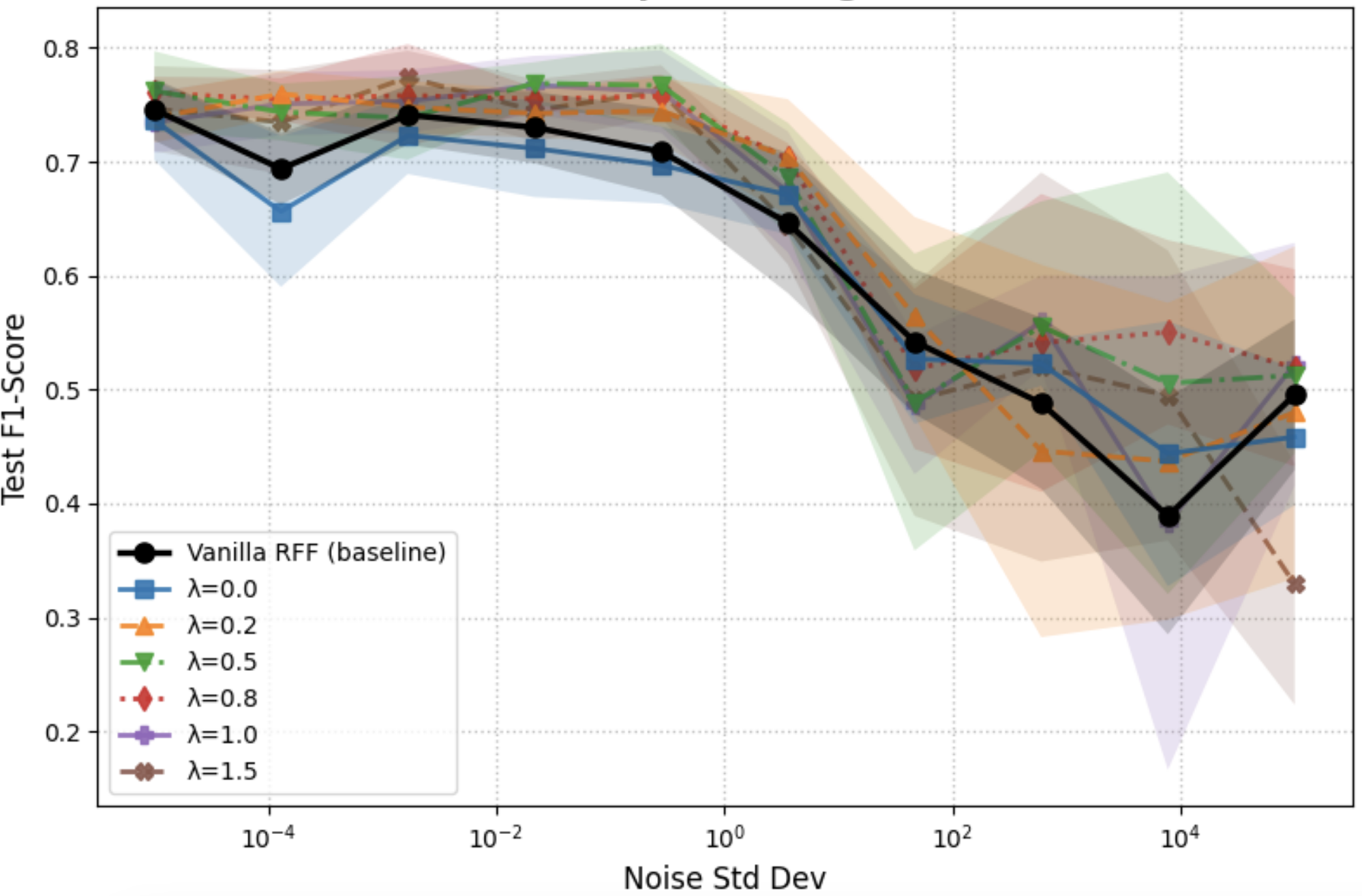
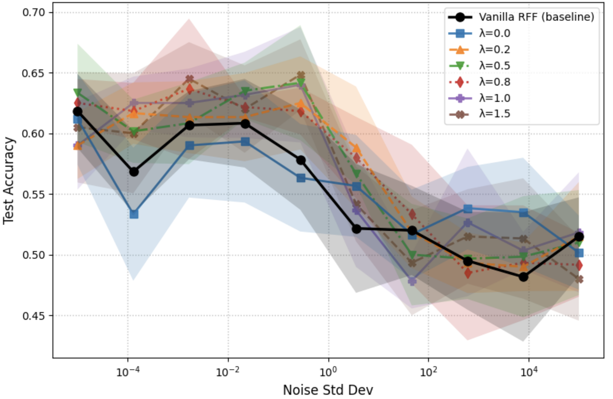
We vary the potential strength $\lambda\in\{0.0,0.2,0.5,0.8,1.0,1.5\}$ and evaluate robustness as input noise increases (x–axis: noise standard deviation on a log scale). Across both metrics (Accuracy and F1), small noise regimes ( $\sigma\!\leq\!10^{-3}$ ) show minimal separation between curves, indicating that the potential has little effect when the signal is clean. As noise grows to the moderate range ( $10^{0}\!\!-\!10^{2}$ ), nonzero potentials consistently outperform the vanilla RFF baseline and $\lambda=0$ , with $\lambda\approx 0.5\!-\!1.0$ yielding the most reliable gains (typically a few points) and smaller variance, suggesting improved stability. In the extreme-noise regime ( $\sigma\!\geq\!10^{3}$ ), performance degrades for all settings and the gaps narrow; very large strengths ( $\lambda\!=\!1.5$ ) can oversmooth and underperform, while small-to-moderate $\lambda$ remains competitive but offers diminishing returns. Overall, a moderate Coulomb/Riesz potential ( $\lambda\approx 0.5\!-\!1.0$ ) provides the best robustness–accuracy trade-off, whereas too weak or too strong potentials are less effective.

F.2 Sentence-Level Classification Benchmarks

Table 7: Statistics of sentence-level and sentence-pair classification datasets used in our experiments. Counts denote the number of examples per split. For sentence-pair tasks, each example consists of a pair of sentences.

Dataset	Train	Dev	Test	Classes	Task
SST-2 Socher et al. (2013)	67,349	872	1,821	2	Sentiment classification
QQP Wang et al. (2019)	363,846	40,430	390,965	2	Duplicate question detection
Rotten Tomatoes Pang and Lee (2005)	8,530	1,066	1,066	2	Sentiment classification

Dataset selection.

We evaluate sentence-level and sentence-pair classification performance on a set of widely used English benchmarks that are standard in prior work on attention mechanisms.

The selected datasets span multiple semantic phenomena and dataset scales, including binary sentiment analysis on SST-2 and Rotten Tomatoes, as well as semantic equivalence detection on the QQP benchmark. Together, these tasks cover both single-sentence and sentence-pair settings, enabling evaluation across varying supervision regimes and levels of linguistic complexity.

Datasets and splits.

SST-2 Socher et al. (2013) is a binary sentiment classification task derived from the Stanford Sentiment Treebank. We use the GLUE version of the dataset, which removes neutral examples and provides sentence-level annotations, and follow the standard GLUE train/dev/test splits.

QQP Wang et al. (2019) (Quora Question Pairs) is a sentence-pair classification task in which each example consists of two questions from Quora annotated for semantic equivalence. We adopt the official GLUE splits and process each question pair by concatenation with a special separator token.

Rotten Tomatoes Pang and Lee (2005) is a sentence-level binary sentiment classification dataset constructed from movie reviews. We use the standard polarity version of the dataset and follow the commonly used train/dev/test splits.

Preprocessing.

We apply minimal preprocessing to preserve the original linguistic structure of each dataset. All text is tokenized using a fixed WordPiece vocabulary, with original casing and punctuation retained. Inputs are truncated or padded to a maximum length of 128 tokens. For sentence-pair inputs in QQP, the two questions are concatenated using a special separator token. No segment embeddings or task-specific features are used unless otherwise stated.

Training protocol.

For each dataset, we train models on the official training split and use the validation split exclusively for model selection and early stopping. Hyperparameters are fixed across all experiments and are not tuned on validation data. For each method, we select the checkpoint that achieves the highest validation accuracy and report performance on the held-out test split using this checkpoint. Test data are never used for hyperparameter selection or model selection.

Evaluation and metrics.

Across all datasets, we report classification accuracy as the primary performance metric. For binary classification tasks (SST-2, QQP, and Rotten Tomatoes), we additionally report micro-, macro-, and weighted $F_{1}$ scores to account for potential class imbalance. To evaluate ranking quality and probabilistic reliability, we also report ROC-AUC, precision–recall AUC, Matthews correlation coefficient (MCC), balanced accuracy, LogLoss, Brier score, and expected calibration error (ECE). All metrics are computed on the test split using the checkpoint selected based on validation performance.

Experimental setup.

Inputs are tokenized using the bert-base-uncased WordPiece tokenizer and truncated or padded to a maximum sequence length of 128 tokens. Models use a two-layer Transformer encoder with hidden size 128, two attention heads, feedforward dimension 256, and $m=256$ random features per head. In our particle-based view, each column of $\bm{\Omega}_{N}\in\mathbb{R}^{H\times d_{k}\times m}$ is a particle, so this corresponds to 256 particles per head (512 per layer; 1024 particles total across the two-layer encoder). Dropout is set to 0.1, and mean pooling is applied over token representations. We use a $\log$ repulsion force between particles.

Training uses a batch size of 64. When kernel optimization is enabled, training proceeds in two phases. In Phase A, the attention feature map parameters $\bm{\Omega}_{N}$ (and optionally layer normalization and value projection parameters) are optimized using an alignment loss objective for up to 10 epochs via particle optimization (SGLD/Langevin dynamics with step size $\eta=2\times 10^{-3}$ and inverse temperature $\beta=50$ , i.e., Gaussian noise scale $\sqrt{2\eta/\beta}$ , plus a repulsion term with $\lambda=10^{-3}$ and gradient clipping at norm 10), while the remaining model parameters are frozen. Column-wise $L_{2}$ norms of $\bm{\Omega}_{N}$ (i.e., per-particle norms) are constrained to 1.5. Training in Phase A stops early if the maximum change in $\bm{\Omega}_{N}$ falls below $10^{-6}$ . In Phase B, the kernel parameters are frozen and the model is trained end-to-end with cross-entropy loss for 10 epochs. For vanilla baselines, only Phase B is used. Optimization in Phase B is performed with Adam using a learning rate of $2\times 10^{-4}$ .

Effect of Kernel Learning.

Tables 1, 2, and 3 quantify the effect of target-alignment kernel learning across SST-2, QQP, and Rotten Tomatoes. On SST-2 (Table 1), where overall performance is near saturation, kernelization yields feature-map-dependent gains. Kernel-porf-softplus attains the best accuracy and MCC (0.8188/0.6376). Several kernel variants improve both discriminative and probabilistic metrics: for example, Kernel-elu increases accuracy from 0.8028 to 0.8108 while simultaneously reducing LogLoss (0.4938 $\rightarrow$ 0.4502) and Brier score (0.1505 $\rightarrow$ 0.1392), and Kernel-softmaxfeat improves accuracy (0.8005 $\rightarrow$ 0.8085) while achieving near-optimal LogLoss (0.4381). Calibration-specific improvements are also evident: Kernel-cos2 yields the lowest Brier score (0.1366), while Kernel-favor achieves the lowest ECE (0.3086). However, not all kernels are uniformly beneficial—Kernel-softplus degrades both Brier and ECE—highlighting sensitivity to the choice of feature map.

On the more challenging QQP task (Table 2), kernel learning provides more consistent benefits across feature maps. Kernel-softmaxfeat is the strongest $Q{=}K$ model (Acc 0.7909, MCC 0.5506), with substantial reductions in LogLoss (0.4625 $\rightarrow$ 0.4354) and Brier score (0.1512 $\rightarrow$ 0.1418), while Kernel-favor achieves the best calibration as measured by ECE (0.4106). Although kernelization roughly doubles training time, it does not affect inference-time complexity, indicating that alignment primarily reshapes representation geometry and probabilistic reliability rather than merely sharpening decision boundaries.

Results on Rotten Tomatoes (Table 3) exhibit similar but more modest trends. Kernel-softmaxfeat achieves the highest accuracy and MCC (0.7167/0.4345) while also attaining the lowest LogLoss (0.5697) and Brier score (0.1929), suggesting that kernel alignment is particularly effective in improving probabilistic calibration on smaller, noisier datasets. As on SST-2, gains vary across feature maps, reinforcing the importance of the kernel choice.

Despite these improvements, Vaswani-style softmax attention remains the strongest performer on QQP. Its advantage stems from explicitly modeling dense all-pairs token interactions through an $\ell\times\ell$ attention matrix, incurring $\mathcal{O}(\ell^{2})$ time and memory complexity in the sequence length $\ell$ . This expressivity is well suited to paraphrase detection, where fine-grained cross-token alignment is critical, but the quadratic scaling limits practicality for longer sequences. In contrast, linear-attention variants trade some modeling capacity for $\mathcal{O}(\ell)$ -type scaling (up to the feature dimension), making them preferable when sequence length or throughput constraints dominate.

Appendix G Appendix

We organize the appendix as follows:

•

In Section G.3, we present the proof of Theorem E.1.
•

In Section G.4 we present the large deviation result of Theorem E.3.

G.1 Notation

We define the notation as follows:

•

$\mathcal{M}(\Omega)$ : The space of measures on the measurable space $(\Omega,\mathcal{B})$ , where $\mathcal{B}$ is the Borel $\sigma$ -algebra on $\Omega$ .
•

$\hat{\mu}\in\mathcal{M}(\Omega)$ : A random (counting) measure, typically representing the realization of the point process. It is a random element in the space of measures on $\Omega$ .
•

$\mu\in\mathcal{M}(\Omega)$ : The deterministic (limiting) measure, often representing the stationary or equilibrium distribution of the point process as $N\to\infty$ .
•

$\mathcal{P}:\Xi\to\mathcal{M}(\Omega)$ : A point process mapping from the probability space $(\Xi,\mathcal{F},\mathbb{P})$ to the space of measures on $\Omega$ .
•

$\nu=\mathbb{P}\circ\mathcal{P}^{-1}$ : The push-forward measure of the point process, governing the randomness of the point process and describing the distribution of realizations of the point process.
•

$\Lambda$ : The intensity measure, defined as

$\Lambda(B)=\mathbb{E}_{\mu\sim\nu}[\mu(B)]\quad\text{for}\quad B\in\mathcal{B},$

where $\mu$ is the random measure associated with a realization of the point process.
•

$\Xi$ : The underlying probability space, often taken as a sample space of configurations for the point process.
•

$\hat{\mu}(B)$ : The counting measure or number of points in a subset $B\in\mathcal{B}$ , corresponding to the realization of the random measure $\hat{\mu}$ .
•

$\mathbb{E}[\cdot]$ : Expectation with respect to the probability measure governing the point process. In this context, it is typically the expectation under $\nu$ , the push-forward measure.
•

$\mu(B)$ : The number of points in the set $B$ as determined by the limiting measure $\mu$ .
•

$X$ : A random variable (or random element) associated with the point process, representing a random realization or observation.
•

$x$ : A realization of the random variable $X$ , i.e., an outcome or observation from the random process.

G.2 Proof of Lemma B.1

Insert $\phi_{\bm{\omega}_{k},b_{k}}(\bm{x})=\sqrt{2}\cos(\bm{\omega}_{k}^{\top}\bm{x}+b_{k})$ into (B.4):

\frac{1}{N}\sum_{k=1}^{N}\phi_{\bm{\omega}_{k},b_{k}}(\bm{x}_{i})\phi_{\bm{\omega}_{k},b_{k}}(\bm{x}_{j})=\frac{2}{N}\sum_{k=1}^{N}\cos(\alpha_{ik})\cos(\alpha_{jk}),\quad\alpha_{ik}\stackrel{{\scriptstyle\mathrm{def}}}{{=}}\bm{\omega}_{k}^{\top}\bm{x}_{i}+b_{k}.

Substituting and swapping finite sums gives

\displaystyle\mathcal{E}_{N}(\bm{\Omega}_{N},\bm{b})=-\frac{2}{n(n-1)N}\sum_{k=1}^{N}\sum_{i\neq j}y_{i}y_{j}\cos(\alpha_{ik})\cos(\alpha_{jk}).

(G.1)

For any $\bm{a},\bm{y}\in\mathbb{R}^{n}$ ,

\displaystyle\sum_{i\neq j}y_{i}y_{j}a_{i}a_{j}=\Big(\sum_{i}y_{i}a_{i}\Big)^{2}-\sum_{i}y_{i}^{2}a_{i}^{2}.

(G.2)

Applying (G.2) with $a_{i}=\cos(\alpha_{ik})$ yields

\sum_{i\neq j}y_{i}y_{j}\cos(\alpha_{ik})\cos(\alpha_{jk})=\big(\bm{y}^{\top}\bm{c}_{k}\big)^{2}-\sum_{i}y_{i}^{2}\cos^{2}(\alpha_{ik}),\quad(\bm{c}_{k})_{i}\stackrel{{\scriptstyle\mathrm{def}}}{{=}}\cos(\alpha_{ik}).

Take expectation over the phases $\bm{b}$ , assumed i.i.d. $\mathrm{Unif}[0,2\pi]$ and independent of $(\bm{\Omega}_{N},\{\bm{x}_{i}\})$ :

\mathbb{E}_{b_{k}}\big[\cos^{2}(\bm{\omega}_{k}^{\top}\bm{x}_{i}+b_{k})\big]\;=\;\tfrac{1}{2}.

Therefore,

\mathbb{E}_{b_{k}}\!\left[\sum_{i}y_{i}^{2}\cos^{2}(\alpha_{ik})\right]\;=\;\tfrac{1}{2}\sum_{i}y_{i}^{2}.

In binary classification ( $y_{i}^{2}=1$ ), this equals $n/2$ and is independent of $\bm{\omega}_{k}$ .

Next, write $u_{ik}\stackrel{{\scriptstyle\mathrm{def}}}{{=}}\bm{\omega}_{k}^{\top}\bm{x}_{i}$ and expand $\cos(u_{ik}+b_{k})=\cos u_{ik}\cos b_{k}-\sin u_{ik}\sin b_{k}.$ Define the vectors $\bm{u}_{k}=(\cos u_{1k},\ldots,\cos u_{nk})^{\top}$ , and $\bm{v}_{k}=(\sin u_{1k},\ldots,\sin u_{nk})^{\top}.$ . Then

\displaystyle\bm{y}^{\top}\bm{c}_{k}=\bm{y}^{\top}\!\big(\cos b_{k}\,\bm{u}_{k}-\sin b_{k}\,\bm{v}_{k}\big)

(G.3)

and

\displaystyle(\bm{y}^{\top}\bm{c}_{k})^{2}=(\cos b_{k})^{2}(\bm{y}^{\top}\bm{u}_{k})^{2}+(\sin b_{k})^{2}(\bm{y}^{\top}\bm{v}_{k})^{2}-2\cos b_{k}\sin b_{k}\,(\bm{y}^{\top}\bm{u}_{k})(\bm{y}^{\top}\bm{v}_{k}).

(G.4)

Taking expectation over $b_{k}$ and using $\mathbb{E}[\cos^{2}b_{k}]=\mathbb{E}[\sin^{2}b_{k}]=\tfrac{1}{2}$ and $\mathbb{E}[\sin b_{k}\cos b_{k}]=0$ , we obtain

\mathbb{E}_{b_{k}}\!\left[(\bm{y}^{\top}\bm{c}_{k})^{2}\right]=\tfrac{1}{2}\Big((\bm{y}^{\top}\bm{u}_{k})^{2}+(\bm{y}^{\top}\bm{v}_{k})^{2}\Big).

Combining the two expectations,

\mathbb{E}_{b_{k}}\!\left[\sum_{i\neq j}y_{i}y_{j}\cos(\alpha_{ik})\cos(\alpha_{jk})\right]=\tfrac{1}{2}\Big((\bm{y}^{\top}\bm{u}_{k})^{2}+(\bm{y}^{\top}\bm{v}_{k})^{2}\Big)-\tfrac{1}{2}\sum_{i}y_{i}^{2},

where the second term is a constant (equal to $n/2$ in the binary case) and thus does not depend on $\bm{\omega}_{k}$ . Summing over $k$ and inserting into (G.1),

\mathbb{E}_{\bm{b}}\!\big[\mathcal{E}_{N}(\bm{\Omega}_{N},\bm{b})\big]=-\frac{1}{n(n-1)N}\sum_{k=1}^{N}\Big((\bm{y}^{\top}\bm{u}_{k})^{2}+(\bm{y}^{\top}\bm{v}_{k})^{2}\Big),

where the equality is up to an additive constant independent of $\bm{\Omega}_{N}$ . Finally, stack columns $\bm{C}=\cos(\bm{X}\bm{\Omega}_{N}^{\!\top})=[\bm{u}_{1}\,\cdots\,\bm{u}_{N}],\;\bm{S}=\sin(\bm{X}\bm{\Omega}_{N}^{\!\top})=[\bm{v}_{1}\,\cdots\,\bm{v}_{N}]$ to write

\sum_{k=1}^{N}\Big((\bm{y}^{\top}\bm{u}_{k})^{2}+(\bm{y}^{\top}\bm{v}_{k})^{2}\Big)=\|\bm{y}^{\top}\bm{C}\|_{2}^{2}+\|\bm{y}^{\top}\bm{S}\|_{2}^{2}.

This yield the stated result

\mathbb{E}_{\bm{b}}\!\big[\mathcal{E}_{N}(\bm{\Omega}_{N},\bm{b})\big]\;\equiv\;-\frac{1}{n^{2}}\left(\big\|\bm{y}^{\top}\cos(\bm{X}\bm{\Omega}_{N}^{\!\top})\big\|_{2}^{2}+\big\|\bm{y}^{\top}\sin(\bm{X}\bm{\Omega}_{N}^{\!\top})\big\|_{2}^{2}\right).

G.3 Proof of Theorems 4.1 and E.1

Proof G.1.

We prove Theorem E.1; Theorem 4.1 follows as the special case $V=V_{\mathcal{D}}$ . We present a proof sketch based on the projected-particle mean-field approach. Specifically, we construct a continuous-time interpolation of the projected Langevin particles and compare it with a reflected Itô diffusion. A mean-field (propagation-of-chaos) estimate is then used to replace the empirical drift with the law-dependent drift. Finally, we identify the corresponding adjoint Fokker–Planck equation together with its Robin boundary condition. We describe the comparison step in some detail, as the reflection term is precisely what gives rise to the boundary condition.

Step 1: identification of the mean-field drift.

For $\mu\in\mathcal{P}(\Omega)$ , define

\displaystyle U[\mu](\bm{\omega})\stackrel{{\scriptstyle\mathrm{def}}}{{=}}V(\bm{\omega})+\lambda\int_{\Omega}g_{s}(\bm{\omega}-\bm{\omega}^{\prime})\,\mu(d\bm{\omega}^{\prime}),\qquad b[\mu](\bm{\omega})\stackrel{{\scriptstyle\mathrm{def}}}{{=}}-\nabla U[\mu](\bm{\omega}).

(G.5)

By compactness of $\Omega$ and the assumed smooth regularization of $g_{s}$ (or the collision-free restriction), there is a constant $L<\infty$ , independent of $N$ , such that for all $\bm{\omega},\widetilde{\bm{\omega}}\in\Omega$ and $\mu,\nu\in\mathcal{P}(\Omega)$ ,

\displaystyle\|b[\mu](\bm{\omega})-b[\nu](\widetilde{\bm{\omega}})\|\leq L\Big(\|\bm{\omega}-\widetilde{\bm{\omega}}\|+W_{1}(\mu,\nu)\Big)\leq L\Big(\|\bm{\omega}-\widetilde{\bm{\omega}}\|+W_{2}(\mu,\nu)\Big).

(G.6)

Let $\mu_{N}^{(-k)}=(N-1)^{-1}\sum_{\ell\neq k}\delta_{\bm{\omega}_{\ell}}$ . Since $g_{s}$ is even and the finite interaction is normalized as $1/(2N(N-1))\sum_{k\neq\ell}g_{s}(\bm{\omega}_{k}-\bm{\omega}_{\ell})$ ,

\displaystyle-N\nabla_{\bm{\omega}_{k}}\mathcal{H}_{N}(\bm{\Omega}_{N})

\displaystyle=-\nabla V(\bm{\omega}_{k})-\frac{\lambda}{N-1}\sum_{\ell\neq k}\nabla g_{s}(\bm{\omega}_{k}-\bm{\omega}_{\ell})=b[\mu_{N}^{(-k)}](\bm{\omega}_{k}).

(G.7)

Moreover $\|b[\mu_{N}^{(-k)}](\bm{\omega}_{k})-b[\mu_{N}](\bm{\omega}_{k})\|\leq C/N$ . Thus the algorithm is the projected Euler scheme for the empirical McKean drift, up to a uniformly vanishing $O(N^{-1})$ self-interaction error.

Step 2: continuous-time embedding and the reflected diffusion comparison.

Construct Brownian motions $\bm{B}_{k}$ so that $\bm{B}_{k}((m+1)\eta_{N})-\bm{B}_{k}(m\eta_{N})=\sqrt{\eta_{N}}\,\bm{\xi}_{k}^{m}$ . Let $\overline{\bm{\omega}}_{k}^{N,\eta}(t)=\bm{\omega}_{k}^{m}$ for $t\in[m\eta_{N},(m+1)\eta_{N})$ . The recursion in (E.2) can be written as

\displaystyle\overline{\bm{\omega}}_{k}^{N,\eta}(m\eta_{N})=\mathcal{P}_{\overline{\Omega}}\!\left(\overline{\bm{\omega}}_{k}^{N,\eta}((m-1)\eta_{N})+\eta_{N}b[\overline{\mu}_{(m-1)\eta_{N}}^{N,(-k)}](\overline{\bm{\omega}}_{k}^{N,\eta}((m-1)\eta_{N}))+\sqrt{2/\beta}\,\Delta\bm{B}_{k}^{m}\right),

(G.8)

where $\overline{\mu}_{t}^{N,(-k)}=(N-1)^{-1}\sum_{\ell\neq k}\delta_{\overline{\bm{\omega}}_{\ell}^{N,\eta}(t)}$ and $\Delta\bm{B}_{k}^{m}=\bm{B}_{k}(m\eta_{N})-\bm{B}_{k}((m-1)\eta_{N})$ . This is the natural cadlag embedding of the projected particle chain.

The limiting continuous reflected particle system associated with (G.8) is

	$\displaystyle d\bm{X}_{k}^{N}(t)$	$\displaystyle=b[\mu_{t}^{N,(-k)}](\bm{X}_{k}^{N}(t))\,dt+\sqrt{2/\beta}\,d\bm{B}_{k}(t)-\bm{n}(\bm{X}_{k}^{N}(t))\,dL_{k}^{N}(t),\qquad\mu_{t}^{N}=\frac{1}{N}\sum_{j=1}^{N}\delta_{\bm{X}_{j}^{N}(t)},$		(G.9)
	$\displaystyle\bm{X}_{k}^{N}(t)$	$\displaystyle\in\overline{\Omega},\qquad L_{k}^{N}(t)\text{ is nondecreasing},\qquad\int_{0}^{T}\mathbf{1}_{\Omega}(\bm{X}_{k}^{N}(t))\,dL_{k}^{N}(t)=0.$		(G.10)

Here $\bm{n}$ is the outward normal, so $-\bm{n}\,dL_{k}^{N}$ is the inward reflection. The Skorokhod problem on a compact convex $C^{2}$ domain has a unique reflected solution, and the projection map in (G.8) is precisely the Euler approximation of this reflected equation. The projected-Euler consistency assumption in the theorem means that, for each fixed $T$ ,

\displaystyle\varepsilon_{N,\eta}(T)\stackrel{{\scriptstyle\mathrm{def}}}{{=}}\mathbb{E}\sup_{0\leq t\leq T}\frac{1}{N}\sum_{k=1}^{N}\|\overline{\bm{\omega}}_{k}^{N,\eta}(t)-\bm{X}_{k}^{N}(t)\|^{2}\longrightarrow 0.

(G.11)

For smooth bounded drifts this follows from the standard Euler–Skorokhod estimate; the condition on $\eta_{N}$ makes the discrete projection error negligible on the mean-field scale.

Step 3: nonlinear reflected process and propagation of chaos.

Let $\bm{X}_{k}(t)$ , $k\geq 1$ , be i.i.d. copies of the nonlinear reflected McKean–Vlasov process

	$\displaystyle d\bm{X}_{k}(t)$	$\displaystyle=b[\mu_{t}](\bm{X}_{k}(t))\,dt+\sqrt{2/\beta}\,d\bm{B}_{k}(t)-\bm{n}(\bm{X}_{k}(t))\,dL_{k}(t),\qquad\mu_{t}=\operatorname{Law}(\bm{X}_{k}(t)),$		(G.12)
	$\displaystyle\bm{X}_{k}(t)$	$\displaystyle\in\overline{\Omega},\qquad\int_{0}^{T}\mathbf{1}_{\Omega}(\bm{X}_{k}(t))\,dL_{k}(t)=0.$		(G.13)

The Lipschitz bound (G.6) gives existence and uniqueness by a fixed-point argument on measure-valued curves. Couple $\bm{X}_{k}^{N}$ and $\bm{X}_{k}$ with the same Brownian motion and the same initial particle. For convex $\Omega$ , the reflection map is monotone:

\displaystyle\big(\bm{X}_{k}^{N}(t)-\bm{X}_{k}(t)\big)\cdot\Big(-\bm{n}(\bm{X}_{k}^{N}(t))\,dL_{k}^{N}(t)+\bm{n}(\bm{X}_{k}(t))\,dL_{k}(t)\Big)\leq 0.

(G.14)

Applying Itô’s formula to $\|\bm{X}_{k}^{N}(t)-\bm{X}_{k}(t)\|^{2}$ , using (G.6), and averaging over $k$ yields

	$\displaystyle e_{N}(t)$	$\displaystyle\stackrel{{\scriptstyle\mathrm{def}}}{{=}}\mathbb{E}\sup_{0\leq r\leq t}\frac{1}{N}\sum_{k=1}^{N}\\|\bm{X}_{k}^{N}(r)-\bm{X}_{k}(r)\\|^{2}$		(G.15)
		$\displaystyle\leq C_{T}\int_{0}^{t}e_{N}(s)\,ds+C_{T}\int_{0}^{t}\mathbb{E}W_{2}^{2}\!\left(\frac{1}{N}\sum_{j=1}^{N}\delta_{\bm{X}_{j}(s)},\mu_{s}\right)ds+\frac{C_{T}}{N^{2}}.$		(G.16)

The last term is the leave-one-out/self-interaction error. Since $\Omega$ is compact and $\bm{X}_{j}(s)$ are i.i.d. with law $\mu_{s}$ ,

\displaystyle a_{N}(T)\stackrel{{\scriptstyle\mathrm{def}}}{{=}}\sup_{0\leq s\leq T}\mathbb{E}W_{2}^{2}\!\left(\frac{1}{N}\sum_{j=1}^{N}\delta_{\bm{X}_{j}(s)},\mu_{s}\right)\longrightarrow 0.

(G.17)

Gronwall’s inequality therefore gives

\displaystyle\sup_{0\leq t\leq T}\mathbb{E}W_{2}^{2}(\mu_{t}^{N},\mu_{t})\leq C_{T}\big(a_{N}(T)+N^{-1}+\varepsilon_{N,\eta}(T)\big)\longrightarrow 0.

(G.18)

This is the propagation-of-chaos statement: any fixed finite subcollection of particles becomes asymptotically independent, and each coordinate has law $\mu_{t}$ .

Step 4: the Girsanov/change-of-measure ingredient.

The preceding synchronous estimate can equivalently be written as a compact-domain change-of-measure estimate. To make this explicit, define

\displaystyle\bm{u}_{k}(t)=\sqrt{\beta/2}\Big(b[\mu_{t}^{N}](\bm{X}_{k}^{N}(t))-b[\mu_{t}](\bm{X}_{k}^{N}(t))\Big).

(G.19)

Novikov’s condition holds because $\Omega$ is compact and the drift is bounded. Hence the exponential martingale

\displaystyle\mathcal{Z}_{T}=\exp\!\left(-\sum_{k=1}^{N}\int_{0}^{T}\bm{u}_{k}(t)\cdot d\bm{B}_{k}(t)-\frac{1}{2}\sum_{k=1}^{N}\int_{0}^{T}\|\bm{u}_{k}(t)\|^{2}dt\right)

(G.20)

defines a probability measure under which $\widetilde{\bm{B}}_{k}(t)=\bm{B}_{k}(t)+\int_{0}^{t}\bm{u}_{k}(s)ds$ are Brownian motions. The relative entropy of this tilted law with respect to the original law is

\displaystyle D_{\mathrm{KL}}(\widetilde{\mathbb{P}}_{N,T}\|\mathbb{P}_{N,T})=\frac{1}{2}\sum_{k=1}^{N}\widetilde{\mathbb{E}}\int_{0}^{T}\|\bm{u}_{k}(t)\|^{2}dt\leq C\,N\int_{0}^{T}\widetilde{\mathbb{E}}W_{2}^{2}(\mu_{t}^{N},\mu_{t})dt.

(G.21)

By Pinsker’s inequality and the bounded diameter of $\Omega$ , this entropy bound gives, at the empirical-measure level,

\displaystyle\mathbb{E}W_{2}^{2}(\mu_{t}^{N,{\mathrm{emp}}},\mu_{t}^{N,{\mathrm{nl}}})\leq\operatorname{diam}(\Omega)^{2}\left(\frac{2}{N}D_{\mathrm{KL}}(\widetilde{\mathbb{P}}_{N,t}\|\mathbb{P}_{N,t})\right)^{1/2},

(G.22)

where $\mu_{t}^{N,{\mathrm{emp}}}$ and $\mu_{t}^{N,{\mathrm{nl}}}$ denote the empirical measures of the empirical-drift and decoupled reflected systems. This quantifies the cost of replacing the particle drift by the law-dependent McKean drift. Combining (G.11), (G.18), (G.22), and the triangle inequality gives

\displaystyle\sup_{0\leq t\leq T}\mathbb{E}W_{2}^{2}\!\left(\frac{1}{N}\sum_{k=1}^{N}\delta_{\bm{\omega}_{k}^{\lfloor t/\eta_{N}\rfloor}},\mu_{t}\right)\longrightarrow 0.

(G.23)

Since $W_{2}$ convergence on compact $\Omega$ implies weak convergence, this proves the empirical-measure convergence in both theorem statements.

Step 5: identification of the McKean–Vlasov PDE and the boundary condition.

Let $\psi\in C^{2}(\overline{\Omega})$ belong to the generator domain of the reflected diffusion, i.e. $\partial_{\bm{n}}\psi=0$ on $\partial\Omega$ . Applying Itô’s formula to $\psi(\bm{X}_{t})$ in (G.12) gives

\displaystyle\frac{d}{dt}\int_{\Omega}\psi(\bm{\omega})\,\mu_{t}(d\bm{\omega})=\int_{\Omega}\left[b[\mu_{t}](\bm{\omega})\cdot\nabla\psi(\bm{\omega})+\beta^{-1}\Delta\psi(\bm{\omega})\right]\mu_{t}(d\bm{\omega}).

(G.24)

The local-time term is $-\partial_{\bm{n}}\psi(\bm{X}_{t})dL_{t}$ , and therefore vanishes for this generator domain. If $\mu_{t}(d\bm{\omega})=\rho_{t}(\bm{\omega})d\bm{\omega}$ , $b[\mu_{t}]=-\nabla U_{t}$ , and $U_{t}=U[\mu_{t}]$ , (G.24) becomes

\displaystyle\frac{d}{dt}\int_{\Omega}\psi\rho_{t}\,d\bm{\omega}=\int_{\Omega}\left[-\nabla U_{t}\cdot\nabla\psi+\beta^{-1}\Delta\psi\right]\rho_{t}\,d\bm{\omega}.

(G.25)

The adjoint of the reflected generator is therefore

\displaystyle\partial_{t}\rho_{t}=-\nabla\cdot(\rho_{t}b[\mu_{t}])+\beta^{-1}\Delta\rho_{t}=\nabla\cdot(\rho_{t}\nabla U_{t})+\beta^{-1}\Delta\rho_{t}\qquad\text{in }\Omega.

(G.26)

To identify the boundary condition, integrate the last display against arbitrary smooth test functions and use Green’s formula. The boundary contribution is

\displaystyle\int_{\partial\Omega}\psi(\bm{\omega})\Big(\rho_{t}(\bm{\omega})b[\mu_{t}](\bm{\omega})-\beta^{-1}\nabla\rho_{t}(\bm{\omega})\Big)\cdot\bm{n}(\bm{\omega})\,dS(\bm{\omega}).

(G.27)

Reflection means that the probability current through $\partial\Omega$ vanishes. Since $b[\mu_{t}]=-\nabla U_{t}$ , this current condition is

\displaystyle\Big(\rho_{t}\nabla U_{t}+\beta^{-1}\nabla\rho_{t}\Big)\cdot\bm{n}=0\qquad\text{on }(0,T]\times\partial\Omega.

(G.28)

For smooth $\rho_{t}$ , (G.28) is exactly the Robin form

\displaystyle\partial_{\bm{n}}\rho_{t}+\beta\rho_{t}\partial_{\bm{n}}U_{t}=0\qquad\text{on }(0,T]\times\partial\Omega,

(G.29)

which is exactly the Robin/no-flux boundary condition generated by the reflected dynamics. The initial condition follows from $\mu_{0}^{N}\Rightarrow\rho_{0}d\bm{\omega}$ . Taking $\psi\equiv 1$ in the weak formulation gives $\int_{\Omega}\rho_{t}=1$ , and nonnegativity follows because $\rho_{t}$ is the density of the law of the reflected process. Finally, sending $\beta\to\infty$ removes the diffusion term and reduces the no-flux condition to $(\rho_{t}\bm{v}_{t})\cdot\bm{n}=0$ , where $\bm{v}_{t}=-\nabla U_{t}$ , yielding the deterministic reflected continuity equation.

G.4 Proof of Theorem E.3

The proof of Theorem E.3 follows standard application of Varadhan’s lemma Ellis (2005). We provide the proof in multiple steps.

G.4.1 Rewrite the Hamiltonian as a functional of $\mu_{N}$

Let $\nu$ denote Lebesgue measure on $\Omega$ and set

\rho\stackrel{{\scriptstyle\mathrm{def}}}{{=}}\;\frac{\nu}{\nu(\Omega)}.

We use $\rho$ as reference probability measure, i.e., $\rho\in\mathcal{P}(\Omega)$ . We also recall the definition of empirical measure $\mu_{N}=\frac{1}{N}\sum_{k=1}^{N}\delta_{\bm{\omega}_{k}}$ . Under the product measure $\rho^{\otimes N}$ on $\Omega^{N}$ , the empirical measure $\mu_{N}$ satisfies Sanov’s theorem: it obeys an LDP on $\mathcal{P}(\Omega)$ with speed $N$ and good rate function

I(\mu)=\operatorname{Ent}(\mu\mid\rho).

(G.30)

Now, define the bounded measurable function

V(\bm{\omega})\stackrel{{\scriptstyle\mathrm{def}}}{{=}}-\frac{1}{n(n-1)}\sum_{0\leq i\neq j\leq n}y_{i}y_{j}\phi_{\bm{\omega}}(\bm{x}_{i})\phi_{\bm{\omega}}(\bm{x}_{j}).

(G.31)

Then by the Monte–Carlo substitution in (B) and the definition (B.4), the empirical loss is exactly a linear functional of $\mu_{N}$ :

\mathcal{E}_{N}(\bm{\Omega}_{N})=-\frac{1}{n(n-1)}\sum_{i\neq j}y_{i}y_{j}\int_{\Omega}\phi_{\bm{\omega}}(\bm{x}_{i})\,\phi_{\bm{\omega}}(\bm{x}_{j})\,\mu_{N}(\mathrm{d}\bm{\omega})=\int_{\Omega}V(\bm{\omega})\,\mu_{N}(\mathrm{d}\bm{\omega}),

(G.32)

Assume the interaction term is of mean-field form (as in the Gibbs law (E.7)):

\mathcal{W}_{N,s}(\bm{\Omega}_{N})\stackrel{{\scriptstyle\mathrm{def}}}{{=}}\frac{1}{2N(N-1)}\sum_{1\leq k\neq\ell\leq N}g_{s}(\bm{\omega}_{k}-\bm{\omega}_{\ell}).

(G.33)

Define the corresponding continuum interaction functional on $\mathcal{P}(\Omega)$ :

\mathcal{W}_{s}(\mu)\stackrel{{\scriptstyle\mathrm{def}}}{{=}}\frac{1}{2}\int_{\Omega}\int_{\Omega}g_{s}(\bm{\omega}-\bm{\omega}^{\prime})\,\mu(\mathrm{d}\bm{\omega})\mu(\mathrm{d}\bm{\omega}^{\prime}).

(G.34)

Then the full empirical Hamiltonian in (B.3) can be written as

\mathcal{H}_{N,s}(\bm{\Omega}_{N})=\mathcal{E}_{N}(\bm{\Omega}_{N})+\lambda\,\mathcal{W}_{N,s}(\bm{\Omega}_{N}).

(G.35)

With this normalization, $\mathcal{W}_{N,s}(\bm{\Omega}_{N})$ converges to $\mathcal{W}_{s}(\mu_{N})$ ; after truncation the difference is only a harmless finite-size correction. To handle possible singularities of the kernel $g_{s}$ at $\bm{0}$ , we introduce a truncation.

G.4.2 Truncation of the interaction kernel and removal of the diagonal constant

The Columb/Riesz kernel $g_{s}$ is singular at the origin. In order to work with bounded continuous functionals on $\mathcal{P}(\Omega)$ (so that Varadhan’s lemma applies), we introduce a truncation. For $\varepsilon\geq 0$ define the truncated kernel

\displaystyle g_{s}^{\varepsilon}(\bm{\omega})\stackrel{{\scriptstyle\mathrm{def}}}{{=}}\min\{\|\bm{\omega}\|^{-s},\varepsilon^{-s}\}

(G.36)

and adopt the convention that $g_{s}^{\varepsilon}(\bm{0})$ is the (finite) value of this truncation at $\bm{0}$ . In particular, $g_{s}^{\varepsilon}(\bm{0})=\varepsilon^{-s}$ . Define the truncated empirical interaction by

\mathcal{W}_{N,s}^{\varepsilon}(\Omega_{N})\stackrel{{\scriptstyle\mathrm{def}}}{{=}}\frac{1}{2N(N-1)}\sum_{1\leq k\neq\ell\leq N}g_{s}^{\varepsilon}(\bm{\omega}_{k}-\bm{\omega}_{\ell}),

(G.37)

and the corresponding truncated mean-field interaction functional on $\mathcal{P}(\Omega)$ by

\mathcal{W}_{s}^{\varepsilon}(\mu)\stackrel{{\scriptstyle\mathrm{def}}}{{=}}\frac{1}{2}\int_{\Omega}\int_{\Omega}g_{s}^{\varepsilon}(\bm{\omega}-\bm{\omega}^{\prime})\,\mu(d\bm{\omega})\,\mu(d\bm{\omega}^{\prime}).

(G.38)

For fixed $\varepsilon$ , the map $\mu\mapsto\mathcal{W}_{s}^{\varepsilon}(\mu)$ is continuous on $\mathcal{P}(\Omega)$ since $g_{s}^{\varepsilon}$ is bounded and continuous on $\Omega_{N}$ . Define the truncated energy functional on $\mathcal{P}(\Omega)$ by

\mathcal{H}_{s}^{\varepsilon}(\mu)\stackrel{{\scriptstyle\mathrm{def}}}{{=}}\int_{\Omega}V(\bm{\omega})\,\mu(d\bm{\omega})+\lambda\,\mathcal{W}_{s}^{\varepsilon}(\mu).

(G.39)

and define the truncated empirical Hamiltonian by

\mathcal{H}_{N,s}^{\varepsilon}(\bm{\Omega}_{N})\stackrel{{\scriptstyle\mathrm{def}}}{{=}}\mathcal{E}_{N}(\bm{\Omega}_{N})+\lambda\,\mathcal{W}_{N,s}^{\varepsilon}(\bm{\Omega}_{N}).

(G.40)

Lemma G.2 (Finite-size correction for empirical measures).

For every configuration $\bm{\Omega}_{N}=(\bm{\omega}_{1},\dots,\bm{\omega}_{N})\in\Omega^{N}$ ,

\mathcal{W}_{s}^{\varepsilon}(\mu_{N})=\frac{N-1}{N}\mathcal{W}_{N,s}^{\varepsilon}(\bm{\Omega}_{N})+\frac{g_{s}^{\varepsilon}(\bm{0})}{2N}.

(G.41)

Equivalently,

\mathcal{H}_{N,s}^{\varepsilon}(\bm{\Omega}_{N})=\mathcal{H}_{s}^{\varepsilon}(\mu_{N})+\frac{\lambda}{N-1}\mathcal{W}_{s}^{\varepsilon}(\mu_{N})-\lambda\,\frac{g_{s}^{\varepsilon}(\bm{0})}{2(N-1)}.

(G.42)

In particular, for fixed $\varepsilon>0$ ,

\sup_{\mu\in\mathcal{P}(\Omega)}\left|\frac{\lambda}{N-1}\mathcal{W}_{s}^{\varepsilon}(\mu)\right|\leq\frac{|\lambda|\,\varepsilon^{-s}}{2(N-1)}.

Thus replacing $\mathcal{H}_{N,s}^{\varepsilon}(\bm{\Omega}_{N})$ by $\mathcal{H}_{s}^{\varepsilon}(\mu_{N})$ changes the normalized logarithmic Laplace limits below by $o(1)$ at speed $N$ when $\beta_{N}/N\to 1$ and by $o(1)$ at speed $\beta_{N}$ when $\beta_{N}/N\to\infty$ .

Proof G.3.

Since $\mu_{N}=\frac{1}{N}\sum_{k=1}^{N}\delta_{\bm{\omega}_{k}}$ , we have

\mathcal{W}_{s}^{\varepsilon}(\mu_{N})=\frac{1}{2}\frac{1}{N^{2}}\sum_{k,\ell=1}^{N}g_{s}^{\varepsilon}(\bm{\omega}_{k}-\bm{\omega}_{\ell})=\frac{1}{2}\frac{1}{N^{2}}\sum_{k\neq\ell}g_{s}^{\varepsilon}(\bm{\omega}_{k}-\bm{\omega}_{\ell})+\frac{g_{s}^{\varepsilon}(\bm{0})}{2N}.

The off-diagonal term equals

\frac{N-1}{N}\,\frac{1}{2N(N-1)}\sum_{k\neq\ell}g_{s}^{\varepsilon}(\bm{\omega}_{k}-\bm{\omega}_{\ell})=\frac{N-1}{N}\mathcal{W}_{N,s}^{\varepsilon}(\bm{\Omega}_{N}),

which proves (G.41). Solving this identity for $\mathcal{W}_{N,s}^{\varepsilon}$ and adding the linear term $\mathcal{E}_{N}=\int V\,d\mu_{N}$ gives (G.42). The uniform bound follows from $0\leq g_{s}^{\varepsilon}\leq\varepsilon^{-s}$ . The deterministic constant in (G.42) is absorbed into the partition function. The remaining tilt is uniformly $O(1/N)$ ; after multiplication by $\beta_{N}$ and division by the relevant speed, its contribution is $O(1/N)$ both in the thermal scale $\beta_{N}\sim N$ and in the zero-temperature scale $\beta_{N}$ .

Lemma G.2 shows that the $N(N-1)$ -normalized Hamiltonian and the mean-field functional $\mathcal{H}_{s}^{\varepsilon}(\mu_{N})$ have the same logarithmic Laplace limits at the speeds used below. The diagonal constant is absorbed by the partition function, and the remaining finite-size tilt is uniformly negligible. In what follows we therefore use the asymptotically equivalent representation

\mathbb{P}_{N,\beta_{N}}^{\varepsilon}(\mathrm{d}\bm{\Omega}_{N})\asymp\frac{1}{\widetilde{Z}_{N,\beta_{N}}^{\varepsilon}}\exp\!\big(-\beta_{N}\,\mathcal{H}_{s}^{\varepsilon}(\mu_{N})\big)\,\rho^{\otimes N}(\mathrm{d}\bm{\Omega}_{N}),

where $\asymp$ denotes equivalence of the normalized logarithmic Laplace limits at the relevant speed.

G.4.3 Case $\beta_{N}/N\to 1$

Assume $\beta_{N}/N\to 1$ and write $\beta_{N}=N\alpha_{N}$ with $\alpha_{N}=O_{N}(1)$ . We can rewrite the truncated Gibbs law as a tilt by $\mathcal{H}_{s}^{\varepsilon}(\mu_{N})$ :

\mathbb{P}^{\varepsilon}_{N,\beta_{N}}(d\Omega_{N})\propto\exp\!\big(-N\alpha_{N}\,\mathcal{H}_{s}^{\varepsilon}(\mu_{N})\big)\,\rho^{\otimes N}(\mathrm{d}\bm{\Omega}_{N}).

(G.43)

Let $F:\mathcal{P}(\Omega)\to\mathbb{R}$ be bounded and continuous. We leverage Varadhan’s lemma (Ellis, 2005, p. 51), a rigorous formulation of the Laplace principle (or the saddle point technique) applied to measures satisfying a large deviations property:

Lemma G.4 (Varadhan’s Lemma Ellis (2005)).

Suppose a sequence $\{Q_{N}\}_{N=1}^{\infty}$ of probability measures on $\mathcal{X}$ satisfies a large deviations property with rate function $I(x)$ . Let $F:\mathcal{X}\to\mathbb{R}$ be a continuous function that satisfies the tail condition

\displaystyle\lim_{L\to\infty}\limsup_{N\to\infty}\frac{1}{N}\log\int_{x:F(x)\geq L}\exp\bigl(NF(x)\bigr)\,Q_{N}(dx)=-\infty.

(G.44)

Then

\displaystyle\lim_{N\to\infty}\frac{1}{N}\log\int_{\mathcal{X}}\exp\bigl(NF(x)\bigr)\,Q_{N}(dx)=\sup_{x\in\mathcal{X}}\bigl\{F(x)-I(x)\bigr\}.

(G.45)

To apply Varadhan’s lemma, we must verify the tail condition. Let

Q_{N}\;\stackrel{{\scriptstyle\mathrm{def}}}{{=}}\;\rho^{\otimes N}\circ\mu_{N}^{-1}

denote the push-forward law of the empirical measure $\mu_{N}$ on $\mathcal{P}(\Omega)$ under $\rho^{\otimes N}$ . Concretely, for any measurable $A\subset\mathcal{P}(\Omega)$ ,

Q_{N}(A)=\rho^{\otimes N}\bigl(\{\bm{\Omega}_{N}:\mu_{N}(\bm{\Omega}_{N})\in A\}\bigr).

The tail condition in Varadhan’s lemma for a functional $\Phi:\mathcal{P}(\Omega)\to\mathbb{R}$ reads

\lim_{L\to\infty}\limsup_{N\to\infty}\frac{1}{N}\log\int_{\{\mu:\,\Phi(\mu)\geq L\}}e^{N\Phi(\mu)}\,Q_{N}(d\mu)\;=\;-\infty.

(G.46)

Equivalently, since $\mu_{N}$ has law $Q_{N}$ under $\rho^{\otimes N}$ ,

\lim_{L\to\infty}\limsup_{N\to\infty}\frac{1}{N}\log\mathbb{E}_{\rho^{\otimes N}}\Big[e^{N\Phi(\mu_{N})}\mathbf{1}_{\{\Phi(\mu_{N})\geq L\}}\Big]\;=\;-\infty.

(G.47)

In our application, we use the continuous functional for numerator

\Phi^{\varepsilon}_{N}(\mu)\;\stackrel{{\scriptstyle\mathrm{def}}}{{=}}\;-\Big(\alpha_{N}\,\mathcal{H}_{s}^{\varepsilon}(\mu)+F(\mu)\Big),\qquad\alpha_{N}=\beta_{N}/N\to 1,

(G.48)

and for the denominator the functional

\Psi^{\varepsilon}_{N}(\mu)\;\stackrel{{\scriptstyle\mathrm{def}}}{{=}}\;-\alpha_{N}\,\mathcal{H}_{s}^{\varepsilon}(\mu).

(G.49)

We verify (G.46) for $\Phi^{\varepsilon}_{N}$ . The same argument applies to $\Psi^{\varepsilon}_{N}$ .

To do so, we first show that $\mathcal{H}_{s}^{\varepsilon}$ is bounded for fixed $\varepsilon>0$ . Recall

\mathcal{H}_{s}^{\varepsilon}(\mu)=\int_{\Omega}V(\bm{\omega})\,\mu(\mathrm{d}\bm{\omega})\;+\;\lambda\,\mathcal{W}_{s}^{\varepsilon}(\mu),\quad\text{with}\ \mathcal{W}_{s}^{\varepsilon}(\mu)=\frac{1}{2}\iint g_{s}^{\varepsilon}(\bm{\omega}-\bm{\omega}^{\prime})\,\mu(\mathrm{d}\bm{\omega})\mu(\mathrm{d}\bm{\omega}^{\prime}).

Since $V$ is bounded, for all $\mu\in\mathcal{P}(\Omega)$ ,

$\displaystyle\Big\|\int_{\Omega}V\,\mathrm{d}\mu\Big\|$	$\displaystyle\leq\\|V\\|_{\infty}$	(G.50)
	$\displaystyle=\frac{1}{n(n-1)}\left\\|\sum_{0\leq i\neq j\leq n}y_{i}y_{j}\phi_{\bm{\omega}}(\bm{x}_{i})\phi_{\bm{\omega}}(\bm{x}_{j})\right\\|_{\infty}$	(G.51)
	$\displaystyle\leq\|y_{i}y_{j}\|\left\\|\phi_{\bm{\omega}}(\bm{x}_{i})\\|_{\infty}\\|\phi_{\bm{\omega}}(\bm{x}_{j})\right\\|_{\infty}$	(G.52)
	$\displaystyle\leq L_{\phi}^{2}.$	(G.53)

Moreover, by definition of truncated kernel $g_{s}^{\varepsilon}(\bm{\omega})$ in Eq. (G.36), we have $g_{s}^{\varepsilon}\leq\varepsilon^{-s}$ . Therefore, for any $\mu\in\mathcal{P}(\Omega)$ ,

|\mathcal{W}_{s}^{\varepsilon}(\mu)|=\frac{1}{2}\left|\iint g_{s}^{\varepsilon}(\omega-\omega^{\prime})\,\mu(d\omega)\mu(d\omega^{\prime})\right|\leq\frac{1}{2}\left|\iint\varepsilon^{-s}\,\mu(d\omega)\mu(d\omega^{\prime})\right|=\dfrac{\varepsilon^{-s}}{2}.

(G.54)

Combining (G.51)–(G.54) gives, for all $\mu$ ,

|\mathcal{H}_{s}^{\varepsilon}(\mu)|\leq L_{\phi}^{2}+|\lambda|\,\dfrac{\varepsilon^{-s}}{2}\;\stackrel{{\scriptstyle\mathrm{def}}}{{=}}\;C_{\lambda,\varepsilon}.

(G.55)

Since $F$ is bounded and continuous, define

\|F\|_{\infty}\;\stackrel{{\scriptstyle\mathrm{def}}}{{=}}\;\sup_{\mu\in\mathcal{P}(\Omega)}|F(\mu)|<\infty.

Moreover, since $\alpha_{N}=\mathcal{O}_{N}(1)$ , there exists $N_{0}$ and constant $C>0$ such that for all $N\geq N_{0}$ ,

|\alpha_{N}|\leq C.

(G.56)

Then for all $N\geq N_{0}$ and all $\mu\in\mathcal{P}(\Omega)$ ,

$\displaystyle\|\Phi_{N}(\mu)\|$	$\displaystyle=\left\|-\alpha_{N}\mathcal{H}_{s}^{\varepsilon}(\mu)-F(\mu)\right\|$	(G.57)
	$\displaystyle\leq\|\alpha_{N}\|\,\|\mathcal{H}_{s}^{\varepsilon}(\mu)\|+\|F(\mu)\|$	(G.58)
	$\displaystyle\leq CC_{\lambda,\varepsilon}+\\|F\\|_{\infty}\;\stackrel{{\scriptstyle\mathrm{def}}}{{=}}\;K_{\varepsilon,F},$	(G.59)

where we used (G.55) and (G.56). Thus, $\Phi_{N}$ is bounded above by $K_{\varepsilon,F}$ uniformly in $\mu$ , for all $N\geq N_{0}$ . Similarly, for the denominator functional,

\Psi_{N}(\mu)=-\alpha_{N}\mathcal{H}_{s}^{\varepsilon}(\mu)\leq|\alpha_{N}|\,|\mathcal{H}_{s}^{\varepsilon}(\mu)|\leq CC_{\varepsilon}\;\stackrel{{\scriptstyle\mathrm{def}}}{{=}}\;K_{\varepsilon},\qquad N\geq N_{0}.

(G.60)

Fix any $L>K_{M,F}$ . Then by (G.59), for all $N\geq N_{0}$ ,

\{\mu\in\mathcal{P}(\Omega):\Phi_{N}(\mu)\geq L\}=\varnothing.

Hence the tail integral vanishes, i.e.,

\int_{\{\mu:\Phi_{N}(\mu)\geq L\}}e^{N\Phi_{N}(\mu)}\,Q_{N}(d\mu)=0,\qquad N\geq N_{0}.

Therefore,

\frac{1}{N}\log\int_{\{\mu:\Phi_{N}(\mu)\geq L\}}e^{N\Phi_{N}(\mu)}\,Q_{N}(d\mu)=-\infty,\qquad N\geq N_{0}.

This establishes the tail condition (G.46).

\lim_{L\to\infty}\limsup_{N\to\infty}\frac{1}{N}\log\int_{\{\mu:\Phi_{N}(\mu)\geq L\}}e^{N\Phi_{N}(\mu)}\,Q_{N}(d\mu)=-\infty,

(G.61)

The same reasoning, using (G.60), shows that the tail condition also holds for the denominator functional $\Psi_{N}$ .

Now, by Varadhan’s lemma applied to Sanov’s LDP (G.30), we obtain

	$\displaystyle\lim_{N\to\infty}\frac{1}{N}\log\mathbb{E}_{\rho^{\otimes N}}\!\Big[\exp\big(-N(\alpha_{N}\mathcal{H}_{s}^{\varepsilon}+F)(\mu_{N})\big)\Big]$	$\displaystyle=-\inf_{\mu\in\mathcal{P}(\Omega)}\Big(\mathcal{H}_{s}^{\varepsilon}(\mu)+F(\mu)+\operatorname{Ent}(\mu\mid\rho)\Big),$		(G.62)
	$\displaystyle\lim_{N\to\infty}\frac{1}{N}\log\mathbb{E}_{\rho^{\otimes N}}\!\Big[\exp\big(-N\alpha_{N}\mathcal{H}_{s}^{\varepsilon}(\mu_{N})\big)\Big]$	$\displaystyle=-\inf_{\mu\in\mathcal{P}(\Omega)}\Big(\mathcal{H}_{s}^{\varepsilon}(\mu)+\operatorname{Ent}(\mu\mid\rho)\Big).$		(G.63)

Subtracting (G.63) from (G.62) yields the Laplace principle for $\mu_{N}$ under $\mathbb{P}_{N,\beta_{N}}^{\varepsilon}$ at speed $N$ :

\lim_{N\to\infty}-\frac{1}{N}\log\mathbb{E}_{\mathbb{P}_{N,\beta_{N}}^{\varepsilon}}\!\big[e^{-NF(\mu_{N})}\big]=\inf_{\mu}\Big(F(\mu)+\mathcal{J}^{\varepsilon}_{s}(\mu)\Big),

with

\mathcal{J}^{\varepsilon}_{s}(\mu)=\Big(\mathcal{E}_{s}^{\varepsilon}(\mu)+\operatorname{Ent}(\mu\mid\rho)\Big)-\inf_{\nu\in\mathcal{P}(\Omega)}\Big(\mathcal{E}_{s}^{\varepsilon}(\nu)+\operatorname{Ent}(\nu\mid\rho)\Big).

(G.64)

Since $\mathcal{P}(\Omega)$ is a Polish space and the Laplace principle holds for all $F\in C_{b}(\mathcal{P}(\Omega))$ , Bryc’s inverse Varadhan lemma (see, e.g., (Dembo and Zeitouni, 2009, Theorem 4.4.13)) implies that $(\mu_{N})_{N\geq 1}$ satisfies a large deviation principle with speed $N$ and good rate function $\mathcal{J}_{s}^{\varepsilon}$ .

Finally let $\varepsilon\downarrow 0$ . Because $g_{s}^{\varepsilon}\uparrow g_{s}$ , we have $\mathcal{H}_{s}^{\varepsilon}(\mu)\rightarrow\mathcal{H}_{s}(\mu)$ pointwise (possibly $+\infty$ ), so $\mathcal{H}_{s}$ is lower semi-continuous as a supremum of continuous functions. Standard monotone truncation arguments for Laplace principles yield the same Laplace limit with $\mathcal{H}_{s}$ in place of $\mathcal{H}_{s}^{\varepsilon}$ , and hence the LDP with rate

\mathcal{J}_{s}(\mu)=\Big(\mathcal{H}_{s}(\mu)+\operatorname{Ent}(\mu\mid\rho)\Big)-\inf_{\gamma}\Big(\mathcal{H}_{s}(\gamma)+\operatorname{Ent}(\gamma\mid\rho)\Big).

To convert to $\operatorname{Ent}(\cdot\mid\nu)$ , note that $\operatorname{Ent}(\mu\mid\rho)=\operatorname{Ent}(\mu\mid\nu)+\log\nu(\Omega)$ , and the additive constant cancels when subtracting the infimum. This gives the first bullet of the theorem.

G.4.4 Case $\beta_{N}/N\to\infty$

Fix $\varepsilon\geq 0$ and recall that under the equivalent representation (Lemma G.2),

\mathbb{P}_{N,\beta_{N}}^{\varepsilon}(\mathrm{d}\bm{\Omega}_{N})=\frac{1}{\widetilde{Z}_{N,\beta_{N}}^{\varepsilon}}\exp\!\big(-\beta_{N}\,\mathcal{H}_{s}^{\varepsilon}(\mu_{N})\big)\,\rho^{\otimes N}(\mathrm{d}\bm{\Omega}_{N}),

where the partition function is

\widetilde{Z}_{N,\beta_{N}}^{\varepsilon}\;\stackrel{{\scriptstyle\mathrm{def}}}{{=}}\;\mathbb{E}_{\rho^{\otimes N}}\!\Big[\exp\!\big(-\beta_{N}\,\mathcal{H}_{s}^{\varepsilon}(\mu_{N})\big)\Big].

As before, let

Q_{N}\;\stackrel{{\scriptstyle\mathrm{def}}}{{=}}\;\rho^{\otimes N}\circ\mu_{N}^{-1}

denote the law of $\mu_{N}$ on $\mathcal{P}(\Omega)$ under the reference measure $\rho^{\otimes N}$ .

We notice that Sanov probabilities are negligible at speed $\beta_{N}/N\rightarrow\infty$ . The key point is that $Q_{N}$ satisfies an LDP at speed $N$ , so any $Q_{N}$ -probability is at worst $\exp(-cN)$ , which is negligible on the scale $\beta_{N}\gg N$ .

Lemma G.5 (Sanov scale is negligible at speed $\beta_{N}$ ).

Assume $\beta_{N}/N\to\infty$ . Then for every nonempty open set $U\subset\mathcal{P}(\Omega)$ ,

\lim_{N\to\infty}\frac{1}{\beta_{N}}\log Q_{N}(U)=0.

Proof G.6.

Since $Q_{N}(U)\leq 1$ , we have $\limsup_{N\to\infty}\frac{1}{\beta_{N}}\log Q_{N}(U)\leq 0$ .

For the lower bound, note that $\rho$ has full support on $\Omega$ and the set $\{\mu\in\mathcal{P}(\Omega):\operatorname{Ent}(\mu\mid\rho)<\infty\}$ is dense in $\mathcal{P}(\Omega)$ for the weak topology, so any nonempty open $U$ contains some $\mu$ with finite entropy. Hence

\inf_{\mu\in U}\operatorname{Ent}(\mu\mid\rho)<\infty.

By the lower bound in Sanov’s theorem, for open $U$ ,

\liminf_{N\to\infty}\frac{1}{N}\log Q_{N}(U)\;\geq\;-\inf_{\mu\in U}\operatorname{Ent}(\mu\mid\rho)\;>\;-\infty.

Therefore,

\liminf_{N\to\infty}\frac{1}{\beta_{N}}\log Q_{N}(U)=\liminf_{N\to\infty}\frac{N}{\beta_{N}}\cdot\frac{1}{N}\log Q_{N}(U)\;\geq\;0,

because $N/\beta_{N}\to 0$ and $\frac{1}{N}\log Q_{N}(U)$ is bounded below along a subsequence by a finite constant. Combining with the $\limsup\leq 0$ gives the desired limit $0$ .

Now, define the (truncated) ground state energy

e_{\varepsilon}^{\star}\;\stackrel{{\scriptstyle\mathrm{def}}}{{=}}\;\inf_{\mu\in\mathcal{P}(\Omega)}\mathcal{H}_{s}^{\varepsilon}(\mu).

Since $g_{s}^{\varepsilon}$ and $V$ are bounded, $\mathcal{H}_{s}^{\varepsilon}$ is bounded and continuous on $\mathcal{P}(\Omega)$ , hence $e_{\varepsilon}^{\star}\in\mathbb{R}$ .

Lemma G.7 (Partition function at scale $\beta_{N}$ ).

Under $\beta_{N}/N\to\infty$ ,

\lim_{N\to\infty}\frac{1}{\beta_{N}}\log\widetilde{Z}_{N,\beta_{N}}^{\varepsilon}=-\,e_{\varepsilon}^{\star}.

Proof G.8.

Upper bound. Since $\mathcal{H}_{s}^{\varepsilon}(\mu)\geq e_{\varepsilon}^{\star}$ for all $\mu$ ,

\widetilde{Z}_{N,\beta_{N}}^{\varepsilon}=\mathbb{E}_{\rho^{\otimes N}}\!\Big[e^{-\beta_{N}\mathcal{H}_{s}^{\varepsilon}(\mu_{N})}\Big]\leq e^{-\beta_{N}e_{\varepsilon}^{\star}},

so $\limsup_{N\to\infty}\frac{1}{\beta_{N}}\log\widetilde{Z}_{N,\beta_{N}}^{\varepsilon}\leq-e_{\varepsilon}^{\star}$ .

Lower bound. Fix $\varepsilon>0$ and choose $\mu_{\varepsilon}\in\mathcal{P}(\Omega)$ such that $\mathcal{H}_{s}^{\varepsilon}(\mu_{\varepsilon})\leq e_{\varepsilon}^{\star}+\varepsilon$ . By continuity of $\mathcal{H}_{s}^{\varepsilon}$ there exists a nonempty open neighborhood $U$ of $\mu_{\varepsilon}$ such that

\sup_{\mu\in U}\mathcal{H}_{s}^{\varepsilon}(\mu)\leq e_{\varepsilon}^{\star}+2\varepsilon.

Then

\widetilde{Z}_{N,\beta_{N}}^{\varepsilon}\geq\mathbb{E}_{\rho^{\otimes N}}\!\Big[\mathbf{1}_{\{\mu_{N}\in U\}}\,e^{-\beta_{N}\mathcal{H}_{s}^{\varepsilon}(\mu_{N})}\Big]\geq e^{-\beta_{N}(e_{\varepsilon}^{\star}+2\varepsilon)}\,Q_{N}(U).

Taking $\log$ and dividing by $\beta_{N}$ yields

\frac{1}{\beta_{N}}\log\widetilde{Z}_{N,\beta_{N}}^{\varepsilon}\geq-(e_{\varepsilon}^{\star}+2\varepsilon)+\frac{1}{\beta_{N}}\log Q_{N}(U).

By Lemma G.5, $\frac{1}{\beta_{N}}\log Q_{N}(U)\to 0$ , hence

\liminf_{N\to\infty}\frac{1}{\beta_{N}}\log\widetilde{Z}_{N,\beta_{N}}^{\varepsilon}\geq-(e_{\varepsilon}^{\star}+2\varepsilon).

Letting $\varepsilon\downarrow 0$ gives the lower bound $\geq-e_{M}^{\star}$ and completes the proof.

Let $F\subset\mathcal{P}(\Omega)$ be closed. Using the ratio representation,

\mathbb{P}_{N,\beta_{N}}^{\varepsilon}(\mu_{N}\in F)=\frac{\mathbb{E}_{\rho^{\otimes N}}\!\big[\mathbf{1}_{\{\mu_{N}\in F\}}\exp\left(-\beta_{N}\mathcal{H}_{s}^{\varepsilon}(\mu_{N})\right)\big]}{\widetilde{Z}_{N,\beta_{N}}^{\varepsilon}}.

On the event $\{\mu_{N}\in F\}$ we have $\exp\big(-\beta_{N}\mathcal{H}_{s}^{\varepsilon}(\mu_{N})\big)\leq\exp\big(-\beta_{N}\inf_{\mu\in F}\mathcal{H}_{s}^{\varepsilon}(\mu)\big)$ , hence

\mathbb{E}_{\rho^{\otimes N}}\!\big[\mathbf{1}_{\{\mu_{N}\in F\}}\exp\left(-\beta_{N}\mathcal{H}_{s}^{\varepsilon}(\mu_{N})\right)\big]\leq\exp\!\Big(-\beta_{N}\inf_{\mu\in F}\mathcal{H}_{s}^{\varepsilon}(\mu)\Big).

Therefore,

\limsup_{N\to\infty}\frac{1}{\beta_{N}}\log\mathbb{P}_{N,\beta_{N}}^{\varepsilon}(\mu_{N}\in F)\leq-\inf_{\mu\in F}\mathcal{H}_{s}^{\varepsilon}(\mu)-\liminf_{N\to\infty}\frac{1}{\beta_{N}}\log\widetilde{Z}_{N,\beta_{N}}^{\varepsilon}.

By Lemma G.7, $\lim_{N}\frac{1}{\beta_{N}}\log\widetilde{Z}_{N,\beta_{N}}^{\varepsilon}=-e_{\varepsilon}^{\star}$ , so

\displaystyle\limsup_{N\to\infty}\frac{1}{\beta_{N}}\log\mathbb{P}_{N,\beta_{N}}^{\varepsilon}(\mu_{N}\in F)\leq-\Big(\inf_{\mu\in F}\mathcal{H}_{s}^{\varepsilon}(\mu)-e_{\varepsilon}^{\star}\Big).

(G.65)

Now, let $G\subset\mathcal{P}(\Omega)$ be open and fix $\mu\in G$ . By continuity of $\mathcal{H}_{s}^{\varepsilon}$ , there exists a nonempty open neighborhood $U\subset G$ of $\mu$ such that

\sup_{\nu\in U}\mathcal{H}_{s}^{\varepsilon}(\nu)\leq\mathcal{H}_{s}^{\varepsilon}(\mu)+\varepsilon.

Then

$\displaystyle\mathbb{P}_{N,\beta_{N}}^{\varepsilon}(\mu_{N}\in G)$	$\displaystyle\geq\mathbb{P}_{N,\beta_{N}}^{\varepsilon}(\mu_{N}\in U)$	(G.66)
	$\displaystyle=\frac{\mathbb{E}_{\rho^{\otimes N}}\!\big[\mathbf{1}_{\{\mu_{N}\in U\}}e^{-\beta_{N}\mathcal{H}_{s}^{\varepsilon}(\mu_{N})}\big]}{\widetilde{Z}_{N,\beta_{N}}^{\varepsilon}}$	(G.67)
	$\displaystyle\geq\frac{e^{-\beta_{N}(\mathcal{H}_{s}^{\varepsilon}(\mu)+\varepsilon)}\,Q_{N}(U)}{\widetilde{Z}_{N,\beta_{N}}^{\varepsilon}}.$	(G.68)

Using the simple bound $\widetilde{Z}_{N,\beta_{N}}^{\varepsilon}\leq e^{-\beta_{N}e_{\varepsilon}^{\star}}$ we obtain

\mathbb{P}_{N,\beta_{N}}^{\varepsilon}(\mu_{N}\in G)\geq\exp\!\Big(-\beta_{N}(\mathcal{H}_{s}^{\varepsilon}(\mu)-e_{\varepsilon}^{\star}+\varepsilon)\Big)\,Q_{N}(U).

Taking $\log$ and dividing by $\beta_{N}$ gives

\liminf_{N\to\infty}\frac{1}{\beta_{N}}\log\mathbb{P}_{N,\beta_{N}}^{\varepsilon}(\mu_{N}\in G)\geq-(\mathcal{H}_{s}^{\varepsilon}(\mu)-e_{\varepsilon}^{\star}+\varepsilon)+\liminf_{N\to\infty}\frac{1}{\beta_{N}}\log Q_{N}(U).

By Lemma G.5, the last term is $0$ , hence

\liminf_{N\to\infty}\frac{1}{\beta_{N}}\log\mathbb{P}_{N,\beta_{N}}^{\varepsilon}(\mu_{N}\in G)\geq-(\mathcal{H}_{s}^{\varepsilon}(\mu)-e_{\varepsilon}^{\star}+\varepsilon).

Letting $\varepsilon\downarrow 0$ and then taking the infimum over $\mu\in G$ yields

\displaystyle\liminf_{N\to\infty}\frac{1}{\beta_{N}}\log\mathbb{P}_{N,\beta_{N}}^{\varepsilon}(\mu_{N}\in G)\geq-\Big(\inf_{\mu\in G}\mathcal{H}_{s,M}(\mu)-e_{\varepsilon}^{\star}\Big).

(G.69)

Combining Eqs. (G.65) and (G.69) and applying Definition (E.2) establishes that $(\mu_{N})_{N\geq 1}$ satisfies an LDP under $\mathbb{P}_{N,\beta_{N}}^{\varepsilon}$ with speed $\beta_{N}$ and good rate function

\mathcal{J}^{\varepsilon}_{s}(\mu)\;\stackrel{{\scriptstyle\mathrm{def}}}{{=}}\;\mathcal{H}_{s}^{\varepsilon}(\mu)-e_{\varepsilon}^{\star}=\mathcal{H}_{s}^{\varepsilon}(\mu)-\inf_{\nu\in\mathcal{P}(\Omega)}\mathcal{H}_{s}^{\varepsilon}(\nu).

Finally, let $\varepsilon\downarrow 0$ . Since $g_{s}^{\varepsilon}\uparrow g_{s}$ , we have $\mathcal{H}_{s}^{\varepsilon}(\mu)\uparrow\mathcal{H}_{s}(\mu)$ pointwise (possibly $+\infty$ ), and

e_{\varepsilon}^{\star}=\inf_{\mu}\mathcal{H}_{s}^{\varepsilon}(\mu)\uparrow\inf_{\mu}\mathcal{H}_{s}(\mu)\stackrel{{\scriptstyle\mathrm{def}}}{{=}}e^{\star}.

Thus $\mathcal{J}^{\varepsilon}_{s}(\mu)\uparrow\mathcal{J}_{s}(\mu)$ pointwise, where

\mathcal{J}_{s}(\mu)\;\stackrel{{\scriptstyle\mathrm{def}}}{{=}}\;\mathcal{H}_{s}(\mu)-e^{\star}=\mathcal{H}_{s}(\mu)-\inf_{\nu\in\mathcal{P}(\Omega)}\mathcal{H}_{s}(\nu),

which is the claimed rate function in the regime $\beta_{N}/N\to\infty$ .

G.4.5 goodness of rate function.

In the first regime, $\operatorname{Ent}(\cdot\mid\ell)$ has compact level sets (Sanov rate is good), and $\mathcal{E}_{s}$ is lower semicontinuous, so $\mathcal{E}_{s}+\operatorname{Ent}(\cdot\mid\ell)$ has compact sublevel sets, hence $\mathcal{J}_{s}$ is good. In the second regime, $\mathcal{E}_{s}$ is lower semicontinuous and the underlying space is bounded, so the sublevel sets of $\mathcal{E}_{s}$ are tight; together with lower semicontinuity this yields goodness.

$\displaystyle\|\Phi_{N}(\mu)\|$	$\displaystyle=\left\|-\alpha_{N}\mathcal{H}_{s}^{\varepsilon}(\mu)-F(\mu)\right\|$	(G.57)
	$\displaystyle\leq\|\alpha_{N}\|\,\|\mathcal{H}_{s}^{\varepsilon}(\mu)\|+\|F(\mu)\|$	(G.58)
	$\displaystyle\leq CC_{\lambda,\varepsilon}+\\|F\\|_{\infty}\;\stackrel{{\scriptstyle\mathrm{def}}}{{=}}\;K_{\varepsilon,F},$	(G.59)

A Coulomb Particle Model for Learning Kernel Attention in Transformers

Abstract

1 Introduction

2 Particle kernel learning

3 Kernelized attention

4 Theoretical results: mean-field limit and large deviation principle

Theorem 4.1 (Projected-particle McKean–Vlasov mean-field limit).

Theorem 4.2 (Large deviations for learned feature measures).

5 Experiments

Additional experiment details.

6 Conclusion

LLM usage statement.

References

Supplementary Material

Appendix A Related work

Appendix B Proposed approach

Lemma B.1 (Empirical KTA equals trigonometric energy with random bias).

B.1 Langevin dynamics for efficiently solving Eq. (B.3)

Appendix C Kernelized attention in transformer architecture

C.1 Alignment for attention kernel.

Appendix D Positive random-feature maps for linearized attention

Positive exponential random features (favor).

Deterministic positive features (ELU+1+1 with floor + ℓ1\ell_{1} renorm).

Softplus features (floor + ℓ1\ell_{1} renorm).

Squared-sigmoid features (ℓ1\ell_{1} renorm).

Softmax-over-features (per-token).

Cosine-squared random features.

PORF-Softplus (orthogonal initialization).

Learning the kernel via alignment/KTA (Phase A).

Appendix E Theoretical results

E.1 Continuity equations and equilibrium distribution

Theorem E.1 (Projected-particle mean-field continuity equation).

E.2 Thermodynamic limit of the equilibrated state in the short-range case, s>ds>d

Definition E.2 (Large Deviation Principle (LDP)).

Theorem E.3 (Large deviations for empirical measures).

Appendix F Numerical Experiments

F.1 Nonlinear synthetic classification: data, estimators, and evaluation protocol

F.1.1 Problem setting.

F.1.2 Baselines and learned feature maps.

F.1.3 Implementation.

F.1.4 Training protocol, metrics, and plots.

F.1.5 Reproducibility and computation.

F.1.6 Results.

F.1.7 Ablation: Coulomb/Riesz interaction strength.

F.2 Sentence-Level Classification Benchmarks

Dataset selection.

Datasets and splits.

Preprocessing.

Training protocol.

Evaluation and metrics.

Experimental setup.

Effect of Kernel Learning.

Appendix G Appendix

G.1 Notation

G.2 Proof of Lemma B.1

G.3 Proof of Theorems 4.1 and E.1

Proof G.1.

Step 1: identification of the mean-field drift.

Step 2: continuous-time embedding and the reflected diffusion comparison.

Step 3: nonlinear reflected process and propagation of chaos.

Step 4: the Girsanov/change-of-measure ingredient.

Step 5: identification of the McKean–Vlasov PDE and the boundary condition.

G.4 Proof of Theorem E.3

G.4.1 Rewrite the Hamiltonian as a functional of μN\mu_{N}

G.4.2 Truncation of the interaction kernel and removal of the diagonal constant

Lemma G.2 (Finite-size correction for empirical measures).

Proof G.3.

G.4.3 Case βN/N→1\beta_{N}/N\to 1

Lemma G.4 (Varadhan’s Lemma Ellis (2005)).

G.4.4 Case βN/N→∞\beta_{N}/N\to\infty

Lemma G.5 (Sanov scale is negligible at speed βN\beta_{N}).

Proof G.6.

Lemma G.7 (Partition function at scale βN\beta_{N}).

Proof G.8.

G.4.5 goodness of rate function.

Deterministic positive features (ELU $+1$ with floor + $\ell_{1}$ renorm).

Softplus features (floor + $\ell_{1}$ renorm).

Squared-sigmoid features ( $\ell_{1}$ renorm).

E.2 Thermodynamic limit of the equilibrated state in the short-range case, $s>d$

G.4.1 Rewrite the Hamiltonian as a functional of $\mu_{N}$

G.4.3 Case $\beta_{N}/N\to 1$

G.4.4 Case $\beta_{N}/N\to\infty$

Lemma G.5 (Sanov scale is negligible at speed $\beta_{N}$ ).

Lemma G.7 (Partition function at scale $\beta_{N}$ ).