CoLaDAG: Compositional Latent Log-ratio DAG Analysis of the Gut Microbiome under Silver Nanoparticle Exposure
Abstract
Directed network analysis of microbiome counts is complicated by compositional sampling, high dimensionality, and limited biological replication. We present CoLaDAG, a fixed-reference latent additive log-ratio (ALR) estimator for generating sparse directed conditional-dependence hypotheses from compositional counts. The method combines a multinomial observation model, a working linear Gaussian structural equation model, nonconvex DC-ADMM optimization, and post-estimation thresholding with greedy acyclic projection. Under simulations aligned with this observation model, CoLaDAG obtained the largest mean exact-direction Matthews correlation and the smallest mean false discovery rate among the evaluated implementations; performance deteriorated under continuous-data and dropout misspecification. In the 12-mouse silver-nanoparticle (AgNP) case study, the 58-node fitted graph was sensitive to block resampling and ALR reference choice: 60 of 284 primary edges attained a mouse-block selection frequency of at least 0.60. The reported orientations and dose-stratified slopes are exploratory, coordinate-specific hypotheses rather than identified causal or exposure effects. The leading stable relations prioritize anaerobic gut taxa for targeted abundance, metabolite, and perturbation studies, but do not establish cross-feeding or toxicological mechanisms.
Keywords: Directed acyclic graphs; Directed conditional dependence; Compositional data analysis; Silver nanoparticles; Gut microbiome.
1 Introduction
Silver nanoparticles (AgNPs) are widely used in medical dressings, antibacterial coatings, textiles, personal-care products, and food-contact materials because of their antimicrobial properties. Their increasing use creates multiple environmental release pathways, including product washing, abrasion, disposal, wastewater treatment, and land application of sewage sludge. For example, nanosilver-containing textiles can release silver nanoparticles into wash water (Benn and Westerhoff, 2008), and model-based exposure assessments suggest that engineered nanomaterials, including AgNPs, can enter aquatic, sediment, and soil compartments after consumer and industrial use (Gottschalk et al., 2009). After release, AgNPs undergo aggregation, dissolution, sulfidation, chlorination, and adsorption to organic matter, which can alter their mobility, persistence, and toxicity (Levard et al., 2012). Wastewater treatment can further retain or transform metallic AgNPs, potentially routing transformed silver species to downstream environments through effluent or sludge management (Kaegi et al., 2011). Because AgNPs are intrinsically antimicrobial, their ecological risk may involve not only conventional toxicity endpoints but also disruption of microbial community structure and function (Choi et al., 2008).
The gut microbiota provides an important window for assessing biological effects of AgNP exposure because it lies at the interface between environmental contact and host physiological response. Orally ingested AgNPs can interact with dietary components, intestinal mucus, epithelial surfaces, and resident microbes, potentially affecting microbial composition, gut immunity, and host metabolic status. Animal studies have reported AgNP-associated gut microbiota disturbance in mice and rats, sometimes accompanied by immune, colitis-related, metabolic, or neurobehavioral changes (van den Brule et al., 2016; Williams et al., 2015; Javurek et al., 2017; Chen et al., 2017; Wang et al., 2022).

1.1 Related work
High-throughput 16S ribosomal RNA (rRNA) sequencing produces count vectors whose totals are governed by sequencing depth rather than absolute microbial load. This places microbiome observations in the compositional-data setting introduced by Aitchison (1982); only ratios among components are directly interpretable. The broader compositional-data literature formalizes this principle through log-ratio coordinate systems, including additive log-ratio (ALR), centered log-ratio (CLR), and isometric log-ratio (ILR) representations (Egozcue et al., 2003; Pawlowsky-Glahn et al., 2015). The sum constraint can induce artificial negative dependence and can make naive Pearson or Spearman correlation networks misleading (Gloor et al., 2017). Consequently, a substantial literature has developed log-ratio and compositional approaches for microbial association analysis. Most established microbiome network methods, including the work most closely related to ours by Tian et al. (2023), focus primarily on inferring undirected graphs based on conditional associations. Sparse Correlations for Compositional data (SparCC) estimates sparse correlations from compositional data using log-ratio arguments (Friedman and Alm, 2012), and Sparse InversE Covariance estimation for Ecological Association Inference (SPIEC-EASI) combines log-ratio transformations with sparse inverse covariance estimation to recover undirected ecological association networks (Kurtz et al., 2015). Related graphical-model approaches build on sparse precision-matrix estimation (Friedman et al., 2008) or on count-based latent-variable formulations for network reconstruction (Chiquet et al., 2019). Microbiome preprocessing also requires care because rarefaction, excessive zeros, and contaminant sequences can affect downstream network structure (McMurdie and Holmes, 2014; Davis et al., 2018). These methods and preprocessing principles are useful for co-occurrence analysis, but their graph edges are not directed and therefore do not directly encode asymmetric conditional-dependence hypotheses. Directed acyclic graph (DAG) structure learning provides a natural language for directed dependence, but standard algorithms were not designed for compositional count observations. Constraint-based methods such as the PC algorithm (Spirtes et al., 2000), score-based methods such as Hill-Climbing (HC) and Tabu search (Heckerman et al., 1995; Scutari, 2010), and hybrid algorithms such as max-min hill-climbing (MMHC) (Tsamardinos et al., 2006) generally assume variables observed in an unconstrained Euclidean space. Moreover, in observational settings, DAG orientations are constrained by Markov equivalence and usually require additional assumptions for identification (Verma and Pearl, 1990); examples include equal error variances in Gaussian structural equation models (SEMs) (Peters and Bühlmann, 2014) or non-Gaussian structural errors (Shimizu et al., 2006). Continuous optimization approaches, including NOTEARS (Zheng et al., 2018) and the variational-inference extension VI-NOTEARS (Brouillard et al., 2020), provide attractive algebraic treatments of acyclicity, but they still do not by themselves resolve multinomial sampling, log-ratio reference dependence, orientation identifiability, and small-sample microbiome settings. Recent work on compositional graphical modeling further emphasizes that reference choices and log-ratio transformations can substantially alter inferred conditional-dependence structure (Tian et al., 2023). Finally, real microbiome network analysis often relies on tuning and resampling because the true graph is unknown. Stability selection provides a general high-dimensional framework for assessing how sensitive selected variables or edges are to resampling and tuning choices (Meinshausen and Bühlmann, 2010). This motivates the mouse-block bootstrap stability checks used in the case study below, while still leaving biological validation as the essential next step. The proposed CoLaDAG estimator targets directed conditional dependence hypotheses rather than definitive causal effects. It uses a multinomial observation model for sequencing counts, a latent ALR representation, and a sparse acyclic SEM in the chosen coordinate system. This design is useful for environmental toxicology because it can move analysis beyond univariate differential abundance and undirected co-occurrence clusters toward interpretable, directional hypotheses about log-ratio dependence patterns under AgNP exposure (Wang et al., 2022).
1.2 Our Contributions
The methodological contribution is the integration of a multinomial observation model, fixed-reference ALR coordinates, constrained DAG estimation, and explicit post-estimation truncation into an auditable hypothesis-screening workflow for compositional counts. The procedure does not provide reference-invariant or causal identification. Its operating characteristics are instead assessed through aligned and misspecified simulations, threshold and initialization diagnostics, reference sensitivity, mouse-block resampling, and exposure-group slope summaries. Accordingly, the real-data application is an exploratory environmental biostatistics analysis rather than a validated causal-discovery procedure.
Figure 2 summarizes the analysis-level structure of CoLaDAG. The key distinction is that sequencing counts are not first converted into an ordinary Euclidean data matrix and then handed to a generic graph learner. Instead, the count layer, latent log-ratio coordinates, sparse acyclic SEM, explicit truncation, and stability summaries are treated as connected parts of one compositional graph-estimation procedure.
| Sequencing counts and sample metadata |
| Multinomial observation layer with fixed-reference ALR coordinates |
| Sparse acyclic SEM fitted by DC-ADMM optimization |
| Final coefficient thresholding and greedy DAG projection |
| Ranked edges, mouse-block stability, reference sensitivity, and dose overlays |
Overall, this study addresses four primary questions:
-
1.
First, under simulations aligned with the proposed count–latent construction and under selected misspecification stress tests, when does CoLaDAG improve graph recovery relative to the evaluated DAG learners, and where does that advantage fail?
-
2.
Second, in the AgNP gut microbiome data, which fixed-reference ALR-coordinate dependence hypotheses are prioritized, and how much exploratory support remains after accounting for the small number of independent mice?
-
3.
Third, what limited descriptive information do time-adjusted pairwise ALR slopes on a restricted global support provide across exposure groups, without treating them as group-specific DAGs or exposure effects?
-
4.
Fourth, how do mouse-block resampling and ALR reference choice constrain the robustness and interpretation of the genus-level real-data graph?
2 Case-study Data and Preprocessing
The data consist of gut microbiome abundance measurements from mouse fecal samples collected in a controlled silver exposure experiment. Four groups were analyzed: a control group and three AgNP exposure groups with nominal daily doses of , , and , administered by oral gavage once daily for 120 days (Wang et al., 2022). The dose labels 0.1Ag, 2Ag, and 40Ag are shorthand for these nominal AgNP exposure groups and are not additional dimensions of the statistical model. Each group contained three mice sampled at days 0, 60, 120, and 230, yielding microbiome samples. After preprocessing and abundance filtering, the primary genus-level network analysis used compositional parts, corresponding to modeled log-ratio nodes. For the statistical model, each observed fecal sample is indexed by a single sample label ; mouse identity, exposure group, and collection day are treated as sample metadata. Let denote the observed count vector for taxon abundances in sample . The total sequencing depth for sample is
Due to the compositional constraint, the observed counts only carry information about relative abundances rather than absolute microbial loads.
Although repeated observations were collected from the same mouse over time, the present graph analysis uses a working likelihood that treats samples as conditionally independent given their latent log-ratio representations. This is a substantial limitation rather than a harmless technical detail: the number of independent biological units is closer to 12 mice than to 48 samples, and the current model does not include mouse-level random effects or temporal dynamics. Accordingly, all real-data network results are interpreted as exploratory ALR-coordinate hypotheses, and the case study does not claim confirmatory group-specific high-dimensional DAG inference. The feasibility of the real-data analysis therefore comes from strong structural restrictions–a fixed ALR coordinate system, sparsity regularization, hard thresholding, acyclic projection, ranked reporting, mouse-block stability checks, and shared-support dose overlays–rather than from having enough independent biological units to estimate an unrestricted 58-node longitudinal or dose-specific DAG.
For the primary genus-level analysis, raw genus counts were first filtered to remove non-informative or ambiguous taxonomic labels, including labels such as “uncultured”, “metagenome”, “unknown”, and “unidentified”. Genera were then retained if their mean relative abundance exceeded and their prevalence was at least 20% of samples. This filtering step produced the 59-part count matrix used in the main DAG comparison. A pseudocount of 0.5 was used to initialize and to construct transformed inputs for baseline methods. Raw counts and sample totals enter the subsequent multinomial likelihood; because the optimization is nonconvex, the pseudocount can nevertheless influence the fitted solution through initialization. Taxa are reported using the labels supplied in the original genus-level count table. Labels containing family names, database-defined group identifiers, bracketed genera, or the word “group” denote taxonomic features rather than confirmed species. Supplementary Table S1 provides readable forms and interpretations for the nonstandard labels appearing in the main real-data displays.
The analysis proceeded through several interconnected stages. We first benchmarked the estimator using model-aligned and deliberately misspecified simulations, then fitted a global genus-level network to generate directed conditional-dependence hypotheses. Because each exposure group contained only three mice, we did not relearn a high-dimensional group-specific DAG. Instead, we summarized time-adjusted pairwise ALR slopes on a prespecified subset of the global support. Mouse-block resampling and alternative ALR denominators were used as descriptive sensitivity analyses.
3 Methodology
3.1 Data Preprocessing and Transformation
Let denote the observed counts for components in sample . The total sequence count,
is determined by sequencing depth rather than absolute microbial load. Because is compositionally constrained, it strictly carries relative abundance information, rendering standard unconstrained multivariate models inappropriate.
To address this, we introduce latent continuous variables via an additive log-ratio (ALR) transformation:
Choosing the th component as the reference, we define
where is the latent composition vector, , satisfying and . The inverse mapping is the standard softmax function:
Conditional on , we model the observed counts using a multinomial distribution:
This explicitly accounts for varying sampling depths and naturally captures the heteroscedasticity inherent in compositional counts.
3.2 Graph Interpretation under Log-ratio Transformations
A central challenge is that log-ratio transformations generally destroy sparse absolute-scale graph structures. Suppose the unobserved absolute log-abundances follow a sparse DAG. The ALR coordinates with reference component are , where
Because each transformed coordinate shares the reference term , variables that are conditionally independent on the absolute scale can become dependent through the common denominator. This densification phenomenon affects both undirected graphs (producing dense precision matrices) and DAGs (altering SEM coefficients and orientations). Consequently, neither ALR nor CLR transformations can be treated as sparsity-preserving operations.
Therefore, our estimand is not a unique causal DAG of unobserved absolute abundances. Instead, for a fixed reference taxon , the fitted target is a sparse weighted adjacency matrix in the working SEM for ALR coordinates:
An edge simply indicates that is a parent of within this specific coordinate system. It does not strictly imply that “taxon affects taxon ” on an absolute scale, which motivates our subsequent reference-node sensitivity analyses to assess skeleton stability.
While this fixed-reference SEM provides a coherent working target for hypothesis generation, it does not theoretically guarantee causal identifiability, global optimization convergence, or exact false-discovery control; the operational performance of our multinomial layer, truncated penalty, and greedy acyclic projection are therefore evaluated empirically below.
3.3 Objective Function
To model directed conditional dependencies among the ALR coordinates, we impose a linear Gaussian structural equation model (SEM) on the latent variables . Let denote a directed acyclic graph (DAG) over nodes with a weighted adjacency matrix . We assume
| (1) |
where represents the parent set of node in . The implemented estimator uses this zero-intercept working SEM and does not center the latent coordinates before graph fitting. Consequently, fitted coefficients can reflect both location and conditional-dependence structure; this modeling restriction is included among the limitations of the real-data analysis. The SEM is not a mechanistic ecological intervention model.
Furthermore, because purely observational linear Gaussian models are subject to Markov equivalence, true edge orientations cannot be strictly identified without additional assumptions (e.g., non-Gaussian errors or equal variances) which we do not impose. Consequently, the orientations returned by CoLaDAG are algorithm-dependent hypotheses driven by the penalized likelihood and acyclicity constraints; the undirected skeleton and sign stability should be viewed as more robust than any single directional edge.
Under the working independence assumption, we optimize the joint criterion for the observed counts and sample-specific latent coordinates. This is a joint optimization criterion rather than a marginal likelihood obtained by integrating out . Up to an additive constant, its log-likelihood part is
| (2) |
The multinomial term retains the compositional sampling constraint and the SEM term supplies a working Gaussian regularizer for the latent coordinates. Sparsity and acyclicity are imposed in the penalized optimization below.
3.4 Directed Graph Estimation with Acyclicity Constraint
Let denote the number of modeled latent log-ratio coordinates. The weighted adjacency matrix encodes directed SEM coefficients, with indicating an edge from node to node . We require this support graph to be acyclic and sparse.
To enforce acyclicity, we use the constrained-likelihood formulation of Yuan et al. (2019). Introducing auxiliary variables , a directed graph is acyclic when its binary support can be represented through the dual constraints
| (3) |
These inequalities rule out directed cycles while preserving the local Markov interpretation of the DAG (Edwards, 2012).
The indicator in (3) is nonconvex and discontinuous. We therefore follow Shen et al. (2012) and use the truncated- surrogate
where controls the approximation. As , converges pointwise to the edge indicator. The relaxed acyclicity constraint becomes
| (4) |
The implementation uses a sparsity penalty rather than a fixed edge budget. Combining the joint likelihood in (2) with the relaxed acyclicity constraints gives
| minimize | (5) | |||
| over | ||||
| subject to | ||||
Here is the sparsity-penalty parameter used by the submitted code. This formulation aligns with large-scale DAG likelihood approaches (Li et al., 2020) while adapting them to latent compositional coordinates.
3.5 Final Thresholding and DAG Projection
Following the DC-ADMM optimization, which yields a continuous coefficient matrix , CoLaDAG applies a hard threshold to determine the final acyclic support. For a final edge threshold (which is distinct from the truncated- penalty parameter ), we define the thresholded candidate matrix:
| (6) |
Candidate edges are then sorted in decreasing order of magnitude . Starting from an empty graph, CoLaDAG greedily adds a candidate directed edge only if doing so does not create a directed cycle. The final estimator retains the original signed coefficient for the selected acyclic edges and sets all other entries to zero. Including this explicit truncation step is essential to counteract the densification phenomenon induced by log-ratio transformations.
4 Simulation Study
We evaluated the proposed method in a controlled latent multinomial DAG benchmark with 100 independent replicates. Each replicate generated a latent DAG with nodes and samples. Candidate edges were sampled with probability , assigned coefficients , and greedily projected to a valid DAG. Pre-scaling SEM residual variances were drawn from . The generated coordinates were divided by the softmax temperature before composition formation; the residual variances on the final ALR scale were therefore . Counts were sampled at fixed sequencing depth .
We compared CoLaDAG with a project-specific VI-NOTEARS-style implementation, PC, MMHC, HC-Huge, and Tabu-Huge. CoLaDAG, PC, MMHC, HC-Huge, and Tabu-Huge received the same latent matrix produced by the preliminary CoLaDAG recovery wrapper; VI-NOTEARS-style jointly estimated its own latent representation from the counts. Thus this comparison evaluates graph learners conditional on the submitted recovery workflow, not six independent end-to-end observation models. Hyperparameters were fixed using separate tuning simulations rather than the 100 assessment seeds; the tuning budgets and their asymmetry are given in Supplementary Section S2. Exact-direction MCC, FDR, and TPR score agreement with the simulated orientation, whereas SHD is computed after conversion to CPDAGs. Because the Gaussian observational model does not identify a unique orientation, CPDAG and skeleton results are the more defensible structural summaries.
| Method | Edges | MCC | FDR | TPR | SHD |
|---|---|---|---|---|---|
| CoLaDAG | |||||
| PC | |||||
| VI-NOTEARS-style | |||||
| Tabu-Huge | |||||
| MMHC | |||||
| HC-Huge |

As shown in Table 1 and Figure 3, CoLaDAG had the largest mean exact-direction MCC and the smallest mean FDR under the aligned latent multinomial mechanism. PC and the VI-NOTEARS-style implementation followed in MCC, whereas the graphical-lasso-screened HC and Tabu searches produced denser graphs and larger CPDAG SHD. These results describe finite-sample behavior under the stated generating mechanism; they do not establish orientation identifiability or uniform superiority.
4.1 Sensitivity Analysis for Log-ratio Sparsity
To illustrate the non-invariance concerns in Section 3.2, we conducted a population-level diagnostic independent of any estimator. Sparse linear Gaussian DAGs were generated under chain, hub, and Erdos–Renyi topologies with absolute-scale dimension . We transformed the exact population covariance into ALR coordinates and into an orthonormal Helmert (ILR) basis, then evaluated precision and order-specific DAG densities at numerical tolerance .
| Topology | Transform | Original DAG density | Precision density | Ordered DAG density | Random-order DAG density |
|---|---|---|---|---|---|
| Chain | ALR | ||||
| Hub | ALR | ||||
| Random | ALR | ||||
| Chain | ILR (Helmert) | ||||
| Hub | ILR (Helmert) | ||||
| Random | ILR (Helmert) |
At the stated tolerance, the transformed precision matrices and sequential DAG factorizations were complete in the reported settings (Table 2). This diagnostic illustrates the potential for severe sparsity loss under the examined references, bases, and coefficient distributions. It motivates sensitivity analysis and explicit thresholding, but does not prove that every log-ratio graph is dense or validate a particular threshold.
4.2 Extended Robustness and Ablation Checks
Supplementary Section S3 reports component ablation, dimension and graph-density experiments, continuous-SEM misspecification, random count dropout, and final threshold sensitivity. The aligned experiments favored CoLaDAG on mean MCC, whereas HC-Huge was substantially better for directly observed continuous SEM data and all methods were near chance after the examined dropout contamination. The supplement therefore maps model-specific operating characteristics rather than confirming a universal method ranking.
5 Real Data Analysis
5.1 Genus-level Graph and Biological Interpretability
To derive biological insights from the real data, we applied CoLaDAG to the genus abundance table, using the most abundant retained genus, Lachnospiraceae_NK4A136_group, as the ALR reference denominator. CoLaDAG identified 284 directed ALR-coordinate edges, whereas the baseline methods selected between 34 and 89 edges under their specified thresholds (Table 3). Given the density of the full support graph, biological interpretation prioritizes the strongest coefficients, supplemented by time-adjusted ALR slope comparisons, mouse-block stability, and reference-node sensitivity analyses.
| Method | Discovered Edges | Network Sparsity |
|---|---|---|
| CoLaDAG (Ours) | ||
| HC-Huge | ||
| PC | ||
| MMHC | ||
| Tabu-Huge | ||
| VI-NOTEARS-style |
The top 10 strongest CoLaDAG coefficients, representing fixed-reference ALR-coordinate dependencies within the fitted SEM, are prioritized in Table 4 for biological interpretation.
| Rank | From | To | Weight | Sign | |
|---|---|---|---|---|---|
| 1 | Intestinimonas | Lachnospiraceae_AC2044_group | 3.5196 | 3.5196 | Positive |
| 2 | Alistipes | Ruminiclostridium_5 | 2.6899 | 2.6899 | Positive |
| 3 | Oscillibacter | Rikenellaceae_RC9_gut_group | 2.6810 | 2.6810 | Positive |
| 4 | Oscillibacter | Lachnospiraceae_AC2044_group | -2.3723 | 2.3723 | Negative |
| 5 | Intestinimonas | Azospirillum_sp._47_25 | 2.0719 | 2.0719 | Positive |
| 6 | Alistipes | Dubosiella | -1.9843 | 1.9843 | Negative |
| 7 | Intestinimonas | Dubosiella | -1.8766 | 1.8766 | Negative |
| 8 | Ruminiclostridium | Parabacteroides | -1.8211 | 1.8211 | Negative |
| 9 | Lachnoclostridium | A2 | 1.7584 | 1.7584 | Positive |
| 10 | Roseburia | Faecalibaculum | 1.6581 | 1.6581 | Positive |
The first-ranked relation was from Intestinimonas to the Lachnospiraceae AC2044 group, a database-defined genus-level feature. It attained mouse-block selection frequency 0.70 and conditional sign agreement 0.857, providing stronger exploratory support than rank alone. The exact labels Oscillibacter and Rikenellaceae RC9 gut group were verified against the supplied genus table. Their fitted relation may reflect coordinated change, but the present compositional analysis cannot distinguish shared responses to diet, exposure, or host state from microbial exchange or mathematical coupling induced by the common ALR denominator. It should therefore not be interpreted as evidence of direct ecological interaction or cross-feeding. Follow-up studies should combine taxon-specific quantification with SCFA and other metabolite measurements.
5.2 Mouse-block Stability Analyses
Because the real AgNP data do not have a known ground-truth network, baseline parameters cannot be selected by MCC or FDR. We therefore performed an additional mouse-block bootstrap stability experiment for the score-based HC-Huge and Tabu-Huge baselines. The experiment used the 30 ALR coordinates with the largest variance under the same primary reference taxon, evaluated StARS thresholds and BIC penalty multipliers , and repeated each setting over 25 bootstrap resamples. Each bootstrap replicate sampled the 12 mouse blocks with replacement and retained all time points for a selected mouse. An edge was treated as stable if its empirical selection frequency was at least 0.60. We summarized each setting by the mean number of skeleton edges, mean number of directed graph edges, number of stable directed edges, and an instability proxy , where is the bootstrap selection probability of edge .
The most stable configuration was Tabu-Huge with StARS threshold 0.10 and BIC multiplier 3, yielding a mean of 14.16 directed edges, 4 stable edges, and the lowest instability score (0.0222). The corresponding HC-Huge setting selected 15.80 directed edges on average and 3 stable edges. Compared with ordinary sample-level resampling, mouse-block bootstrap gives a more conservative view of edge stability and reinforces the need to treat all real-data graphs as exploratory.
| Method | StARS | factor | Bootstrap reps. | Mean skeleton edges | Mean graph edges | Stable edges | Instability |
|---|---|---|---|---|---|---|---|
| Tabu-Huge | 0.10 | 3 | 25 | 28.56 | 14.16 | 4 | 0.0222 |
| HC-Huge | 0.10 | 3 | 25 | 33.60 | 15.80 | 3 | 0.0242 |
| Tabu-Huge | 0.10 | 2 | 25 | 33.96 | 16.36 | 4 | 0.0253 |
| HC-Huge | 0.10 | 2 | 25 | 34.32 | 16.80 | 3 | 0.0264 |
| HC-Huge | 0.10 | 1 | 25 | 31.24 | 18.76 | 6 | 0.0272 |
| Tabu-Huge | 0.15 | 3 | 25 | 76.64 | 18.32 | 5 | 0.0280 |
We also performed a reduced-iteration CoLaDAG mouse-block diagnostic. Twenty resamples drew the 12 mouse blocks with replacement and retained all four observations from each selected block. The diagnostic used smaller DC and ADMM iteration caps than the primary fit for computational feasibility and therefore does not estimate the stability of an identical refitting procedure. All 20 scripts returned a graph, although the current wrapper does not expose inner-solver fallback counts. The resampled graphs contained 603.15 edges on average, compared with 284 in the primary fit, revealing substantial tuning and resampling sensitivity. Among the 284 primary edges, the median selection frequency was 0.45; 60 edges had frequency at least 0.60, and 37 also had conditional sign agreement at least 0.80. The leading primary Intestinimonas Lachnospiraceae_AC2044_group edge had selection frequency 0.70 and conditional sign agreement 0.857. These frequencies are descriptive stability diagnostics, not selection-adjusted error probabilities.
| Quantity | Value |
| Successful bootstrap fits | 20 / 20 |
| Primary edges | 284 |
| Mean bootstrap edges | 603.15 |
| Median primary-edge selection frequency | 0.45 |
| Primary edges with selection frequency | 60 |
| Above threshold with sign agreement | 37 |
5.3 Dose-stratified Analyses
The AgNP design naturally motivates comparison across the control, 0.1Ag, 2Ag, and 40Ag groups. Each exposure group contains only three mice and 12 longitudinal observations, so relearning a separate 58-node DAG in each group would be unstable. We therefore used a restricted shared-support display. The global CoLaDAG fit supplied candidate orientations, after which only its 80 largest absolute coefficients were considered. Within each exposure group, we fitted a separate regression of the child ALR coordinate on one candidate parent and collection-time indicators. These quantities are time-adjusted pairwise ALR slopes, not conditional SEM coefficients, because the remaining parents of the child were not included. Slopes with were retained and at most 20 were displayed per group. The threshold and top-20 cap are visualization rules, not dose-specific DAG tuning parameters. Displayed arrows retain the global orientation solely to identify the source and target coordinates.


These displays do not represent four independently estimated DAGs. The heatmap is the primary comparison; the network panels retain the global source–target labels for context. Slopes that remain large in several groups suggest a recurrent pairwise log-ratio pattern, whereas sign or magnitude differences are descriptive candidates for a future mouse-level interaction analysis. The full ranked lists are reported in Supplementary Section S4 and in the accompanying CSV file.
The primary denominator was the Lachnospiraceae NK4A136 group. Under this reference, the Intestinimonas-to-Dubosiella slope was 2.752 in Control, in 0.1Ag, 0.076 in 2Ag, and in 40Ag. The Alistipes–Ruminiclostridium group 5 slope was positive in all four groups (1.261, 0.516, 1.013, and 0.886, respectively). The first pattern illustrates heterogeneity, whereas the second illustrates a more recurrent relation; neither establishes a dose response. Each group contains only three mice, and the naive intervals ignore support selection, within-mouse dependence, and multiplicity. We therefore report these slopes as a biological follow-up list rather than as significant exposure-specific effects. The pooled “Other” category is excluded from biological interpretation because it is not a taxon.
6 Discussion and Conclusion
Under simulations aligned with its multinomial–latent construction, CoLaDAG achieved the largest mean exact-direction MCC and the smallest mean FDR among the evaluated implementations. The advantage did not generalize to every setting: HC-Huge performed better for the unaligned continuous SEM, and random count dropout reduced all methods to near-chance recovery. The simulation evidence is therefore model-specific rather than a universal ranking.
In the AgNP study, the genus-level graph prioritized coordinate-specific hypotheses involving Intestinimonas, Alistipes, Oscillibacter, Ruminiclostridium group 5, and Lachnospiraceae AC2044 group. Only 60 of 284 primary edges reached mouse-block selection frequency 0.60, 37 also met the sign-agreement criterion, and alternative ALR references produced materially different graphs. These findings support a ranked follow-up list, not stable or reference-invariant microbial interactions.
Time-adjusted pairwise ALR slopes showed both heterogeneous and recurrent patterns across exposure groups, but three mice per group cannot establish dose response or exposure effects. Together with the zero-intercept working SEM, nonconvex optimization, repeated-measure treatment in the primary likelihood, and unresolved genus-group labels, these limitations make CoLaDAG a fixed-reference screening procedure for directed log-ratio hypotheses rather than a microbial causal-map estimator. Independent abundance, metabolite, and perturbation studies are required for biological validation.
Declaration of Generative AI and AI-assisted Technologies
During preparation of this work, the authors used OpenAI Codex to support language editing, code auditing, and manuscript formatting. The authors reviewed and edited all resulting material and take full responsibility for the content of the publication.
Funding
Shuyan Chen was supported by the Youth Innovation Fund of the University of Science and Technology of China (No. WK2040250119).
References
- The statistical analysis of compositional data. Journal of the Royal Statistical Society: Series B (Methodological) 44 (2), pp. 139–177. Cited by: §1.1.
- Nanoparticle silver released into water from commercially available sock fabrics. Environmental Science & Technology 42 (11), pp. 4133–4139. External Links: Document Cited by: §1.
- Differentiable causal discovery from interventional data. In Advances in Neural Information Processing Systems, Vol. 33, pp. 21865–21877. Cited by: §1.1.
- The effects of orally administered Ag, TiO2 and SiO2 nanoparticles on gut microbiota composition and colitis induction in mice. NanoImpact 8, pp. 80–88. External Links: Document Cited by: §1.
- Variational inference for sparse network reconstruction from count data. In Proceedings of the 36th International Conference on Machine Learning (ICML), pp. 1162–1171. Cited by: §1.1.
- The inhibitory effects of silver nanoparticles, silver ions, and silver chloride colloids on microbial growth. Water Research 42 (12), pp. 3066–3074. External Links: Document Cited by: §1.
- Simple statistical identification and removal of contaminant sequences in marker-gene and metagenomics data. Microbiome 6 (1), pp. 226. Cited by: §1.1.
- Introduction to graphical modelling. Springer Science & Business Media. Cited by: §3.4.
- Isometric logratio transformations for compositional data analysis. Mathematical Geology 35 (3), pp. 279–300. Cited by: §1.1.
- Sparse inverse covariance estimation with the graphical lasso. Biostatistics 9 (3), pp. 432–441. Cited by: §1.1.
- Inferring correlation networks from genomic survey data. PLoS computational biology 8 (9), pp. e1002687. Cited by: §1.1.
- Microbiome datasets are compositional: and this is not optional. Frontiers in microbiology 8, pp. 2224. Cited by: §1.1.
- Modeled environmental concentrations of engineered nanomaterials (TiO2, ZnO, Ag, CNT, fullerenes) for different regions. Environmental Science & Technology 43 (24), pp. 9216–9222. External Links: Document Cited by: §1.
- Learning bayesian networks: the combination of knowledge and statistical data. Machine learning 20 (3), pp. 197–243. Cited by: §1.1.
- Gut dysbiosis and neurobehavioral alterations in rats exposed to silver nanoparticles. Scientific Reports 7, pp. 2822. External Links: Document Cited by: §1.
- Behavior of metallic silver nanoparticles in a pilot wastewater treatment plant. Environmental Science & Technology 45 (9), pp. 3902–3908. External Links: Document Cited by: §1.
- Sparse and compositionally robust inference of microbial ecological networks. PLoS computational biology 11 (5), pp. e1004226. Cited by: §1.1.
- Environmental transformations of silver nanoparticles: impact on stability and toxicity. Environmental Science & Technology 46 (13), pp. 6900–6914. External Links: Document Cited by: §1.
- Likelihood ratio tests for a large directed acyclic graph. Journal of the American Statistical Association 115 (531), pp. 1304–1319. Cited by: §3.4.
- Waste not, want not: why rarefying microbiome data is inadmissible. PLoS Computational Biology 10 (4), pp. e1003531. Cited by: §1.1.
- Stability selection. Journal of the Royal Statistical Society: Series B (Statistical Methodology) 72 (4), pp. 417–473. Cited by: §1.1.
- Modeling and analysis of compositional data. John Wiley & Sons. Cited by: §1.1.
- Identifiability of gaussian structural equation models with equal error variances. The Annals of Statistics 42 (3), pp. 971–1012. Cited by: §1.1.
- Learning bayesian networks with the bnlearn r package. Journal of Statistical Software 35 (3), pp. 1–22. Cited by: §1.1.
- Likelihood-based selection and sharp parameter estimation. Journal of the American Statistical Association 107 (497), pp. 223–232. Cited by: §3.4.
- A linear non-gaussian acyclic model for causal discovery. Journal of Machine Learning Research 7, pp. 2003–2030. Cited by: §1.1.
- Causation, prediction, and search. MIT press. Cited by: §1.1.
- Compositional graphical lasso resolves the impact of parasitic infection on gut microbial interaction networks in a zebrafish model. Journal of the American Statistical Association 118 (543), pp. 1500–1514. Cited by: §1.1.
- The max-min hill-climbing bayesian network structure learning algorithm. Machine learning 65 (1), pp. 31–78. Cited by: §1.1.
- Dietary silver nanoparticles can disturb the gut microbiota in mice. Particle and Fibre Toxicology 13, pp. 38. External Links: Document Cited by: §1.
- Equivalence and synthesis of causal models. In Proceedings of the Sixth Annual Conference on Uncertainty in Artificial Intelligence, pp. 255–270. Cited by: §1.1.
- Changes in gut microbiota structure: a potential pathway for silver nanoparticles to affect the host metabolism. ACS nano 16 (11), pp. 19002–19012. External Links: Document Cited by: §1.1, §1, §2.
- Effects of subchronic exposure of silver nanoparticles on intestinal microbiota and gut-associated immune responses in the ileum of Sprague-Dawley rats. Nanotoxicology 9 (3), pp. 279–289. External Links: Document Cited by: §1.
- Constrained likelihood for reconstructing a directed acyclic gaussian graph. Biometrika 106 (1), pp. 109–125. Cited by: §3.4.
- DAGs with no tears: continuous optimization for structure learning. In Advances in Neural Information Processing Systems, Vol. 31, pp. 9472–9483. Cited by: §1.1.
Supplementary Material for
CoLaDAG: Compositional Latent Log-ratio DAG Analysis of the Gut Microbiome under Silver Nanoparticle Exposure
Shuyan Chen, Ziliang Shen, and Xinlei Wang
S1 Interpretation of Taxonomic Labels
The real-data tables and network figures preserve the machine-readable labels from the supplied genus-level count table. Underscores are separators and do not indicate additional taxonomic resolution. The interpretations below decode the labels used in the displays; they are not species-level reannotations.
| Original label | Readable form | Interpretation and reporting level |
|---|---|---|
| Lachnospiraceae_NK4A136_group | Lachnospiraceae NK4A136 group | Database-defined group within Lachnospiraceae; genus-level group label and the primary ALR denominator. |
| Rikenellaceae_RC9_gut_group | Rikenellaceae RC9 gut group | Database-defined RC9 gut group within Rikenellaceae; genus-level group label, not a confirmed species. |
| Lachnospiraceae_AC2044_group | Lachnospiraceae AC2044 group | Database-defined AC2044 group within Lachnospiraceae; genus-level group label. |
| Lachnospiraceae_UCG-001 | Lachnospiraceae UCG-001 | Database-defined uncultured genus-level cluster within Lachnospiraceae. |
| Ruminococcaceae_UCG-004 | Ruminococcaceae UCG-004 | Database-defined uncultured genus-level cluster within Ruminococcaceae. |
| Ruminococcaceae_UCG-010 | Ruminococcaceae UCG-010 | Database-defined uncultured genus-level cluster within Ruminococcaceae. |
| Ruminococcaceae_UCG-014 | Ruminococcaceae UCG-014 | Database-defined uncultured genus-level cluster within Ruminococcaceae. |
| Ruminococcaceae_NK4A214_group | Ruminococcaceae NK4A214 group | Database-defined NK4A214 group within Ruminococcaceae; genus-level group label. |
| [Eubacterium]_xylanophilum_group | Eubacterium xylanophilum group | Bracketed legacy genus assignment associated with the xylanophilum group; not a species-level identification. |
| [Ruminococcus]_gnavus_group | Ruminococcus gnavus group | Bracketed legacy genus assignment associated with the gnavus group; not a species-level identification. |
| Ruminiclostridium_5 | Ruminiclostridium group 5 | Numbered database subgroup within Ruminiclostridium; not a formal species name. |
| Ruminiclostridium_6 | Ruminiclostridium group 6 | Numbered database subgroup within Ruminiclostridium; not a formal species name. |
| Ruminococcus_1 | Ruminococcus group 1 | Numbered database subgroup within Ruminococcus; genus-level feature label. |
| Azospirillum_sp._47_25 | Azospirillum sp. 47-25 | Supplied feature identifier; the present data do not independently validate a species or strain. |
| A2 | A2 | Unresolved database feature label retained from the supplied taxonomy table. |
| ASF356 | ASF356 | Altered Schaedler Flora member identifier; a strain/group label rather than a genus name. |
| Other | Other | Pooled residual category; not a single biological taxon and not used for mechanistic interpretation. |
S2 Computational Implementation and Comparator Configuration
S2.1 Implemented target, initialization, and stopping rules
The submitted workflow optimizes the joint count–latent-coordinate criterion given in the main manuscript. It is a joint optimization over the sample-specific rather than a marginal likelihood. The implemented working SEM has no intercept and the latent coordinates are not centered before graph fitting. This restriction is disclosed because it can cause coefficients to absorb coordinate location as well as conditional-dependence structure.
For a count matrix with rows and parts, coordinates are modeled. The default initialization is
where is the final, prespecified reference column. The initial residual variances are the empirical coordinate variances, truncated below at 0.05. Raw counts and sample totals enter the multinomial likelihood after initialization; the 0.5 pseudocount is also used to construct continuous ALR inputs for baseline methods.
Each sample-specific latent vector is updated by BFGS with an analytic gradient. The outer wrapper stops when the relative change in its recorded objective is below or the configured cap is reached. The graph solver receives absolute and relative ADMM tolerances of . The analysis scripts also apply fixed DC and ADMM caps, so reaching a cap is not equivalent to a convergence certificate. The optimization is nonconvex and no global optimum is claimed.
S2.2 Parameter configurations and tuning provenance
| Method | Input | Configuration | Output convention |
|---|---|---|---|
| CoLaDAG, simulation | Counts and recovered latent ALR coordinates | Recovery: , , 3 DC and 20 ADMM iterations. Refinement: , , , 10 DC and 50 ADMM iterations; final threshold . | means |
| CoLaDAG, real data | Counts and recovered latent ALR coordinates | Recovery: , , 5 DC and 20 ADMM iterations. Refinement: , , , 10 DC and 50 ADMM iterations; final threshold . | means |
| HC-Huge / Tabu-Huge | Shared recovered ALR matrix | Graphical-lasso skeleton selected by StARS 0.20; Gaussian BIC score with ; absent skeleton arcs blacklisted. | bnlearn fromto converted without transposition |
| PC | Shared recovered ALR matrix | Gaussian correlation tests with ; default stable-PC options. | Returned arcs converted to the common adjacency convention |
| MMHC | Shared recovered ALR matrix | Default bnlearn::mmhc configuration. | Returned arcs converted without transposition |
| VI-NOTEARS-style | Multinomial counts | Project-specific variational implementation; , 10 outer iterations, 500 inner iterations, final threshold 0.50, and greedy DAG projection. | Row source, column target |
The HC-Huge and Tabu-Huge StARS/BIC choices were examined in a truth-based grid at using two tuning seeds. The VI-NOTEARS-style value of and its threshold were selected on one separate default simulation. PC and MMHC used the stated defaults. These tuning budgets are not symmetric; the manuscript therefore reports a comparison of the submitted implementations rather than a method-independent ranking. None of the 100 primary assessment seeds was used to select these settings. Real-data parameters were not selected using an unknown graph truth. The threshold is an operational screening choice and is not presented as an error-controlling cutoff.
Directed MCC, FDR, and TPR score the exact simulated orientation. SHD is evaluated after converting the estimated and simulated DAGs to CPDAGs. The unit test constructs and checks metric calculation, graph conversion, edge-list writing, and plotting. Correcting an earlier unintended transpose in the bnlearn conversion required regeneration of the affected outputs.
S2.3 Optimization blocks and complexity
For , the negative multinomial component is
| (S1) |
and the zero-intercept SEM component is
| (S2) |
Given , BFGS minimizes the smooth joint objective over each . Given , the residual-variance update is
The truncated surrogate
is handled by difference-of-convex iterations. ADMM alternates nodewise ridge updates for , weighted soft thresholding for the split coefficient matrix, least-squares updates for nonnegative ordering variables, projection of acyclicity slacks onto the nonnegative orthant, and scaled-dual updates. The continuous coefficient matrix is finally thresholded at and greedily projected to a DAG in decreasing absolute-coefficient order.
Let be the number of BFGS evaluations. A dense outer latent sweep costs time and memory. The direct ADMM formulation stores slack and dual arrays indexed by and therefore requires working memory. Its ordering-variable least-squares problems have rows and columns; without cached factorizations this gives a conservative time bound per ADMM sweep. Nodewise ridge solves add at most time. These are implementation bounds, not claims of optimal algorithmic complexity.
S2.4 Initialization sensitivity and numerical reporting
One default and nine jittered starts were evaluated in an aligned simulation. Jittered latent and graph initial values used standard deviation 0.10.
| Start | Edges | MCC | Jaccard to default | Final objective |
|---|---|---|---|---|
| 1 | 22 | 0.577 | 1.000 | 7,881,881.391 |
| 2 | 23 | 0.604 | 0.800 | 7,881,880.782 |
| 3 | 24 | 0.589 | 0.769 | 7,882,138.519 |
| 4 | 23 | 0.604 | 0.800 | 7,881,904.771 |
| 5 | 23 | 0.604 | 0.800 | 7,881,952.590 |
| 6 | 20 | 0.745 | 0.680 | 7,882,071.531 |
| 7 | 24 | 0.589 | 0.769 | 7,882,214.882 |
| 8 | 25 | 0.575 | 0.741 | 7,882,129.516 |
| 9 | 24 | 0.589 | 0.769 | 7,882,214.223 |
| 10 | 23 | 0.604 | 0.800 | 7,881,895.727 |
Support Jaccard similarity ranged from 0.680 to 1.000 and MCC from 0.575 to 0.745, indicating moderate local-solution sensitivity. Every outer wrapper in this diagnostic stopped after two iterations. The current scripts catch some inner-solver errors and can return the previous graph; therefore a returned graph must not automatically be interpreted as a numerically converged fit.
S2.5 Computing environment and archive
The archived session records R 4.4.2 on 64-bit Windows 11 (build 26200). The workstation is a Lenovo 82JU with an AMD Ryzen 7 5800H processor (8 physical, 16 logical cores; nominal maximum clock 3.2 GHz) and 15.9 GB RAM. Analyses were run without a documented distributed-computing backend. The current session file does not capture the complete contributed-package version set; this is a reproducibility limitation that should be remedied with a lockfile in any public release.
The accompanying reproducibility ZIP contains the manuscript-facing R scripts, processed toy/analysis data, simulation summaries, real-data edge tables, figures, fixed seeds, and the entry point R/00_run_submission_pipeline.R. The latest archived driver status verified_existing verifies packaged outputs but does not claim that all analyses were rerun in that invocation. A clean rerun should preserve solver logs and fail rather than silently accept an inner-solver fallback.
S2.6 Implementation and Optimization Strategy
The submitted implementation initializes with pseudocount ALR coordinates, and with zero matrices, and residual variances with the empirical coordinate variances truncated below at 0.05. Conditional on , each sample-specific latent vector is updated by the Broyden–Fletcher–Goldfarb–Shanno (BFGS) algorithm using an analytic gradient. Residual variances are then updated from the nodewise squared residuals, followed by DC and ADMM graph updates. The outer wrapper stops when the relative change in its recorded objective is below or its iteration limit is reached; the graph solver receives absolute and relative ADMM tolerances of . The overall problem is nonconvex. In the 10-start diagnostic, support Jaccard similarity to the default start ranged from 0.680 to 1.000 and exact-direction MCC ranged from 0.575 to 0.745 after excluding diagonal entries from the confusion matrix, indicating moderate rather than negligible initialization sensitivity.
For dense matrices, one outer latent-coordinate sweep requires operations and storage, where is the number of BFGS objective/gradient evaluations. The implemented ADMM graph block uses acyclicity slack and dual arrays. Its direct ordering-variable least-squares updates give a conservative worst-case bound of time per ADMM sweep and working memory; the nodewise ridge updates contribute at most additional time. These bounds explain why the , 12-mouse analysis is treated as a heavily regularized screening calculation.
All parameter values, iteration caps, comparator settings, initialization diagnostics, and reproducibility instructions are reported in Supplementary Section S2. Because the effective biological sample size is 12, neither the tuning parameters nor turn the case study into confirmatory high-dimensional graph inference.
S3 Extended Simulations and Robustness Checks
S3.1 Sample size and sequencing depth
The aligned sensitivity experiments used and 10 independent replicates per setting. The table reports CoLaDAG and the strongest comparator by mean MCC; complete method-by-setting rows are included in the CSV archive.
| Setting | CoLaDAG MCC | Best comparator | Comparator MCC | CoLaDAG FDR |
|---|---|---|---|---|
| PC | 0.520 | |||
| PC | 0.509 | |||
| PC | 0.410 | |||
| PC | 0.564 | |||
| PC | 0.442 | |||
| Tabu-Huge | 0.369 |
CoLaDAG was not uniformly best: PC had a slightly larger mean MCC at . The results describe operating characteristics near the aligned benchmark rather than a fixed method ordering.
S3.2 Unaligned continuous SEM and dropout
The continuous stress test generated directly observed SEM variables with Gaussian, heavy-tailed , or centered exponential errors. There was no multinomial observation layer. Each setting used and 20 replicates.
| Error | Method | Edges | MCC | FDR |
|---|---|---|---|---|
| Gaussian | HC-Huge | 14.75 | 0.093 | |
| Gaussian | CoLaDAG | 6.25 | 0.394 | |
| Heavy-tailed | HC-Huge | 14.35 | 0.143 | |
| Heavy-tailed | CoLaDAG | 7.00 | 0.452 | |
| Centered exponential | HC-Huge | 15.30 | 0.150 | |
| Centered exponential | CoLaDAG | 7.05 | 0.380 |
The score-based baseline was substantially better in this unaligned setting. This negative result prevents generalizing the aligned-model advantage to directly observed continuous SEM data.
After multinomial sampling, the dropout experiment independently set observed nonzero counts to zero with probability 0, 0.10, or 0.30. Each setting used and 10 replicates.
| Dropout | Method | Edges | MCC | FDR |
|---|---|---|---|---|
| 0 | CoLaDAG | 28.7 | 0.424 | |
| 0 | PC | 28.4 | 0.480 | |
| 0.10 | CoLaDAG | 6.1 | 0.925 | |
| 0.10 | PC | 45.9 | 0.922 | |
| 0.30 | CoLaDAG | 10.7 | 0.893 | |
| 0.30 | PC | 47.9 | 0.925 |
All evaluated methods were near chance after 10% or 30% dropout. The present observation model has no structural-zero or zero-inflation component.
S3.3 Component ablation
The ablation used 30 replicates with . The oracle fit received simulated latent coordinates and is an unattainable reference. The observed-ALR fit used pseudocount log ratios without latent recovery.
| Variant | Edges | MCC | FDR | TPR | SHD |
|---|---|---|---|---|---|
| Oracle latent coordinates + DAG | 26.80 | 0.261 | 0.598 | 19.27 | |
| Observed ALR + DAG | 26.30 | 0.320 | 0.537 | 23.70 | |
| Recovered coordinates, no final threshold | 26.57 | 0.320 | 0.547 | 22.07 | |
| Full CoLaDAG | 25.87 | 0.305 | 0.544 | 21.77 |
Among implementable variants, full CoLaDAG had the largest mean MCC and the smallest mean FDR and SHD. The improvements over observed ALR were modest at the examined sequencing depth.
S3.4 Dimension and graph density
For the dimension experiment, with edge probability . For the density experiment, and edge probability for . Settings used and 20 replicates.
| Setting | CoLaDAG MCC / FDR | Best comparator | Comparator MCC / FDR |
|---|---|---|---|
| Dimension | 0.597 / 0.306 | PC | 0.424 / 0.518 |
| Dimension | 0.570 / 0.330 | PC | 0.338 / 0.619 |
| Dimension | 0.504 / 0.417 | PC | 0.333 / 0.636 |
| Density | 0.700 / 0.252 | Tabu-Huge | 0.550 / 0.484 |
| Density | 0.573 / 0.341 | PC | 0.360 / 0.594 |
| Density | 0.435 / 0.459 | PC | 0.237 / 0.661 |
CoLaDAG had the largest mean MCC and smallest mean FDR in these six aligned settings, while performance declined with dimension and density.
S3.5 Final-threshold sensitivity
The latent recovery and continuous graph output were held fixed within each replicate while only the final threshold was varied (30 replicates, ).
| Threshold | Edges | MCC | FDR | TPR | SHD |
|---|---|---|---|---|---|
| 0.00 | 26.23 | 0.573 | 0.319 | 0.541 | 22.07 |
| 0.05 | 26.23 | 0.573 | 0.319 | 0.541 | 22.07 |
| 0.10 | 26.23 | 0.573 | 0.319 | 0.541 | 22.07 |
| 0.20 | 26.23 | 0.573 | 0.319 | 0.541 | 22.07 |
| 0.30 | 25.57 | 0.579 | 0.305 | 0.538 | 21.80 |
| 0.40 | 23.83 | 0.582 | 0.279 | 0.522 | 21.57 |
| 0.50 | 22.10 | 0.591 | 0.243 | 0.509 | 21.13 |

Increasing the threshold reduced mean edge count and FDR while increasing MCC and reducing SHD, at the cost of lower TPR. This experiment describes a precision–recall trade-off; it does not select or validate the real-data threshold .
S4 Real-data Reporting Details
S4.1 Mouse-block diagnostic budgets
The primary real-data recovery/refinement budgets were 5/20 and 10/50 DC/ADMM iterations, respectively. The 20 CoLaDAG block-resampling fits used reduced budgets of 3/15 and 6/30. The resulting frequencies are therefore approximate sensitivity diagnostics. Baseline block tuning used 25 resamples for each configuration and retained all four observations for every selected mouse.
S4.2 Reference-denominator refits
The reference-sensitivity analysis used the same CoLaDAG parameters and final as the primary fit. For each candidate denominator, the raw count matrix was reordered before the multinomial likelihood was evaluated. Pseudocount ALR coordinates were constructed for the transformed-data comparators and for CoLaDAG initialization. Pairwise graph comparisons were restricted to taxa present as non-reference coordinates in both fits.
S4.3 Reference-node Sensitivity Analysis
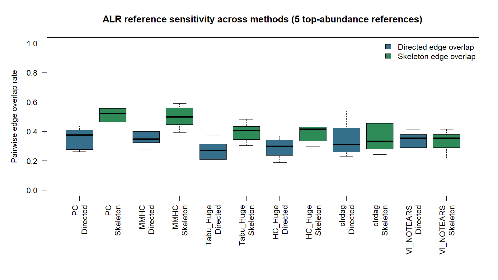
A natural concern in ALR-based compositional modeling is that the inferred network may depend on the arbitrary choice of the denominator taxon. To directly assess this issue, we conducted a reference-node sensitivity analysis on the real gut microbiome data. Specifically, we selected the five most abundant retained compositional parts, Lachnospiraceae_NK4A136_group, Other, Bacteroides, Alistipes, and Muribaculum, and used each of them in turn as the ALR reference. For each reference choice, we refit all directed graph learning methods and compared the resulting graphs pairwise on the common non-reference taxa. This comparison avoids artificially penalizing a method simply because the current reference taxon is excluded from the ALR coordinate system.
Table S10 summarizes the resulting pairwise structural Hamming distances (SHD), edge-overlap rates, and reference-stable core skeleton counts. Under the aligned tuning protocol, the CoLaDAG graphs varied substantially in density across references, from 284 directed edges with Lachnospiraceae_NK4A136_group as denominator to 684 directed edges with Other as denominator. CoLaDAG had mean directed and skeleton overlap rates of 0.346 and 0.368, respectively; 355 skeleton edges appeared in at least three of the five reference choices and 92 appeared under all five choices. These large core counts must be interpreted together with the high graph densities: they do not imply reference-invariant directed effects. PC and MMHC showed higher mean skeleton overlap with much sparser graphs. Overall, the sensitivity analysis confirms that ALR-coordinate graphs are materially reference-dependent and that skeleton-level summaries are more defensible than single-reference edge orientations.
| Method | Directed SHD | Skeleton SHD | Directed overlap | Skeleton overlap | Core edges | Core edges |
|---|---|---|---|---|---|---|
| CoLaDAG | 451.0 | 430.8 | 0.346 | 0.368 | 355 | 92 |
| PC | 51.3 | 26.4 | 0.356 | 0.522 | 38 | 17 |
| MMHC | 42.6 | 29.6 | 0.349 | 0.497 | 41 | 17 |
| Tabu-Huge | 96.4 | 70.2 | 0.257 | 0.396 | 66 | 23 |
| HC-Huge | 91.1 | 70.3 | 0.283 | 0.396 | 67 | 22 |
| VI-NOTEARS-style | 34.7 | 34.7 | 0.330 | 0.330 | 29 | 7 |
As presented in Table 3 in the main text, the primary genus-level analysis produced different graph densities across methods. CoLaDAG selected the largest candidate edge set in this audited count-likelihood run, whereas PC, MMHC, VI-NOTEARS-style, HC-Huge, and Tabu-Huge selected sparser candidate graphs under their specified thresholds. We do not use the full 284-edge CoLaDAG graph as the main display because such a plot is difficult to interpret. Instead, the ranked-edge table in Table 4 in the main text, the exposure-group weight heatmap in Figure 4 in the main text, the retained network overlay in Figure 5 in the main text, and the reference-sensitivity analysis in Table S10 provide more interpretable views of the same fitted procedure.
From an ecological perspective, the CoLaDAG genus-level network highlights several large fitted log-ratio coefficients that can be used to prioritize follow-up checks. The mouse-block analysis retained only 60 of 284 primary edges at selection frequency 0.60, with 37 additionally meeting the sign-agreement criterion. The ranked examples are therefore descriptive coefficient hypotheses rather than stable edge discoveries. The largest absolute coefficients involved Intestinimonas, Alistipes, Oscillibacter, Ruminiclostridium group 5, Rikenellaceae RC9 gut group, and Lachnospiraceae AC2044 group. Because the ALR denominator is Lachnospiraceae_NK4A136_group, no directed edge incident to that reference taxon is estimable in the primary graph. These coefficients should be treated as coordinate-specific prioritization signals, not as evidence of taxon-level biological mechanisms. The most defensible biological payoff is therefore a ranked validation plan: quantify the named taxa with targeted assays, measure candidate fermentation products, and test whether the relations persist after accounting for mouse and time in a larger experiment.
S4.4 Dose-group slope construction
The dose displays do not refit group-specific DAGs. The 80 largest absolute coefficients from the global CoLaDAG fit define a restricted candidate list. For each candidate and group, the submitted script fits
The reported quantity is , a time-adjusted pairwise ALR slope. It is not a conditional SEM coefficient because the other parents of the child are absent. Slopes with are retained and at most 20 are displayed per group. The conventional intervals below treat 12 observations as independent and ignore support selection and multiplicity; with only three mice per group, they are descriptive only.
| Group | Rank | From | To | Estimate (standard error) | Naive 95% interval |
|---|---|---|---|---|---|
| Control | 1 | Intestinimonas | Dubosiella | 2.752 (0.780) | [0.908, 4.597] |
| Control | 2 | Intestinimonas | Rikenellaceae_RC9_gut_group | 2.123 (1.254) | [-0.842, 5.089] |
| Control | 3 | Intestinimonas | Ruminococcaceae_UCG-004 | 1.764 (1.030) | [-0.671, 4.198] |
| Control | 4 | Alistipes | Ruminiclostridium_5 | 1.261 (0.319) | [0.506, 2.015] |
| Control | 5 | Intestinimonas | Azospirillum_sp._47_25 | 1.207 (1.486) | [-2.308, 4.721] |
| Control | 6 | Sphingomonas | Rikenellaceae_RC9_gut_group | 1.184 (0.847) | [-0.819, 3.188] |
| Control | 7 | Oscillibacter | Angelakisella | 1.174 (0.996) | [-1.180, 3.528] |
| Control | 8 | Other | Rikenellaceae_RC9_gut_group | 1.100 (0.702) | [-0.561, 2.760] |
| Control | 9 | Alistipes | Bacteroides | 1.078 (0.287) | [0.401, 1.756] |
| Control | 10 | Desulfovibrio | Lachnospiraceae_UCG-001 | 1.059 (0.727) | [-0.660, 2.778] |
| Control | 11 | Oscillibacter | Rikenellaceae_RC9_gut_group | 1.058 (1.115) | [-1.579, 3.694] |
| Control | 12 | Ruminiclostridium | Rikenellaceae_RC9_gut_group | 1.051 (1.103) | [-1.558, 3.660] |
| Control | 13 | Lachnospiraceae_FCS020_group | Tyzzerella | 1.050 (0.368) | [0.179, 1.920] |
| Control | 14 | Alistipes | Dubosiella | 1.046 (0.378) | [0.153, 1.940] |
| Control | 15 | Desulfovibrio | [Eubacterium]_xylanophilum_group | 1.042 (0.637) | [-0.464, 2.547] |
| Control | 16 | Ruminococcaceae_UCG-014 | Dubosiella | 0.991 (0.178) | [0.570, 1.413] |
| Control | 17 | Lachnoclostridium | Lachnospira | 0.980 (0.902) | [-1.152, 3.113] |
| Control | 18 | Ruminiclostridium | [Eubacterium]_xylanophilum_group | -0.903 (0.852) | [-2.919, 1.112] |
| Control | 19 | Sphingomonas | Faecalibacterium | 0.884 (0.473) | [-0.234, 2.001] |
| Control | 20 | Ruminococcaceae_UCG-014 | Lachnospiraceae_AC2044_group | 0.855 (0.362) | [-0.001, 1.711] |
| 0.1Ag | 1 | Intestinimonas | Lachnospiraceae_UCG-001 | -2.075 (0.978) | [-4.388, 0.238] |
| 0.1Ag | 2 | Other | Mucispirillum | -1.856 (0.909) | [-4.006, 0.293] |
| 0.1Ag | 3 | Ruminococcaceae_NK4A214_group | Lachnospiraceae_AC2044_group | 1.788 (0.543) | [0.504, 3.072] |
| 0.1Ag | 4 | Intestinimonas | Lachnospiraceae_AC2044_group | 1.747 (1.250) | [-1.209, 4.703] |
| 0.1Ag | 5 | Ruminiclostridium_5 | Parabacteroides | 1.587 (0.531) | [0.332, 2.842] |
| 0.1Ag | 6 | Other | Rikenellaceae_RC9_gut_group | 1.569 (0.520) | [0.338, 2.800] |
| 0.1Ag | 7 | Alistipes | Lachnospiraceae_AC2044_group | 1.550 (1.073) | [-0.988, 4.089] |
| 0.1Ag | 8 | Ruminiclostridium_5 | Lachnospiraceae_AC2044_group | 1.538 (1.367) | [-1.693, 4.770] |
| 0.1Ag | 9 | Lachnoclostridium | Lachnospira | 1.506 (0.556) | [0.191, 2.820] |
| 0.1Ag | 10 | Intestinimonas | Azospirillum_sp._47_25 | 1.484 (0.752) | [-0.295, 3.263] |
| 0.1Ag | 11 | Ruminococcaceae_UCG-014 | Lachnospiraceae_AC2044_group | 1.476 (0.792) | [-0.398, 3.349] |
| 0.1Ag | 12 | Other | Helicobacter | 1.474 (1.116) | [-1.166, 4.114] |
| 0.1Ag | 13 | Lachnospiraceae_FCS020_group | Lachnospiraceae_UCG-001 | -1.464 (0.630) | [-2.953, 0.025] |
| 0.1Ag | 14 | Intestinimonas | Ruminococcaceae_UCG-004 | 1.436 (0.610) | [-0.007, 2.879] |
| 0.1Ag | 15 | Ruminococcaceae_NK4A214_group | Lachnospiraceae_UCG-001 | -1.429 (0.547) | [-2.723, -0.135] |
| 0.1Ag | 16 | Intestinimonas | Dubosiella | -1.350 (1.014) | [-3.747, 1.047] |
| 0.1Ag | 17 | Bacteroides | Alloprevotella | 1.331 (0.407) | [0.369, 2.294] |
| 0.1Ag | 18 | Butyricicoccus | Dubosiella | -1.284 (0.283) | [-1.954, -0.614] |
| 0.1Ag | 19 | Oscillibacter | Mucispirillum | 1.238 (0.724) | [-0.474, 2.950] |
| 0.1Ag | 20 | Lachnoclostridium | Lachnospiraceae_UCG-001 | -1.215 (1.060) | [-3.721, 1.292] |
| 2Ag | 1 | Other | Rikenellaceae_RC9_gut_group | 4.207 (1.752) | [0.065, 8.349] |
| 2Ag | 2 | Oscillibacter | Mucispirillum | 3.010 (1.257) | [0.038, 5.982] |
| 2Ag | 3 | Alistipes | Mucispirillum | 2.970 (0.669) | [1.389, 4.551] |
| 2Ag | 4 | Intestinimonas | Lachnospiraceae_AC2044_group | 2.708 (1.324) | [-0.424, 5.839] |
| 2Ag | 5 | Intestinimonas | Azospirillum_sp._47_25 | 2.554 (1.663) | [-1.379, 6.486] |
| 2Ag | 6 | Lachnoclostridium | Marvinbryantia | 2.322 (1.312) | [-0.780, 5.423] |
| 2Ag | 7 | Sphingomonas | Rikenellaceae_RC9_gut_group | 1.980 (0.570) | [0.632, 3.328] |
| 2Ag | 8 | Sphingomonas | ASF356 | 1.946 (0.442) | [0.902, 2.991] |
| 2Ag | 9 | Ruminiclostridium | [Eubacterium]_xylanophilum_group | -1.626 (0.434) | [-2.653, -0.599] |
| 2Ag | 10 | Oscillibacter | [Eubacterium]_xylanophilum_group | -1.567 (0.729) | [-3.291, 0.157] |
| 2Ag | 11 | Faecalibacterium | [Ruminococcus]_gnavus_group | 1.562 (0.909) | [-0.587, 3.712] |
| 2Ag | 12 | Ruminococcaceae_UCG-010 | Parabacteroides | -1.456 (0.466) | [-2.557, -0.355] |
| 2Ag | 13 | Oscillibacter | Butyricicoccus | 1.277 (0.489) | [0.121, 2.433] |
| 2Ag | 14 | Oscillibacter | Rikenellaceae_RC9_gut_group | 1.247 (1.413) | [-2.094, 4.588] |
| 2Ag | 15 | Bacteroides | Alloprevotella | 1.232 (0.554) | [-0.079, 2.543] |
| 2Ag | 16 | Oscillibacter | Bilophila | 1.224 (0.735) | [-0.514, 2.962] |
| 2Ag | 17 | Lachnospiraceae_FCS020_group | Tyzzerella | 1.217 (0.689) | [-0.411, 2.846] |
| 2Ag | 18 | Lachnoclostridium | Lachnospira | 1.216 (1.433) | [-2.172, 4.603] |
| 2Ag | 19 | Ruminococcaceae_UCG-014 | Lachnospiraceae_AC2044_group | -1.122 (0.737) | [-2.864, 0.620] |
| 2Ag | 20 | Roseburia | [Eubacterium]_xylanophilum_group | -1.049 (0.615) | [-2.504, 0.406] |
| 40Ag | 1 | Lachnoclostridium | A2 | 2.092 (1.154) | [-0.636, 4.820] |
| 40Ag | 2 | Intestinimonas | Ruminococcus_1 | 1.973 (0.534) | [0.709, 3.237] |
| 40Ag | 3 | Intestinimonas | Butyricicoccus | 1.921 (0.434) | [0.894, 2.948] |
| 40Ag | 4 | Lachnoclostridium | Lachnospira | 1.891 (0.898) | [-0.232, 4.014] |
| 40Ag | 5 | Lachnoclostridium | Lachnospiraceae_UCG-001 | -1.794 (1.432) | [-5.180, 1.592] |
| 40Ag | 6 | Bilophila | Dubosiella | -1.657 (0.518) | [-2.881, -0.433] |
| 40Ag | 7 | Lachnoclostridium | Marvinbryantia | 1.588 (1.612) | [-2.223, 5.399] |
| 40Ag | 8 | Sphingomonas | Rikenellaceae_RC9_gut_group | 1.374 (0.436) | [0.344, 2.405] |
| 40Ag | 9 | Intestinimonas | Oscillibacter | 1.368 (0.202) | [0.890, 1.846] |
| 40Ag | 10 | Oscillibacter | Butyricicoccus | 1.295 (0.304) | [0.577, 2.013] |
| 40Ag | 11 | Enterorhabdus | Prevotellaceae_UCG-001 | 1.280 (0.137) | [0.956, 1.605] |
| 40Ag | 12 | Roseburia | Faecalibaculum | 1.244 (0.754) | [-0.538, 3.027] |
| 40Ag | 13 | Intestinimonas | Ruminococcaceae_UCG-004 | 1.228 (0.586) | [-0.158, 2.615] |
| 40Ag | 14 | Intestinimonas | Dubosiella | -1.132 (0.858) | [-3.161, 0.898] |
| 40Ag | 15 | Other | Rikenellaceae_RC9_gut_group | 1.111 (0.534) | [-0.152, 2.374] |
| 40Ag | 16 | Sphingomonas | Faecalibacterium | 1.092 (0.195) | [0.631, 1.553] |
| 40Ag | 17 | Lachnospiraceae_FCS020_group | Lachnospiraceae_UCG-001 | 1.081 (0.783) | [-0.771, 2.934] |
| 40Ag | 18 | Lachnoclostridium | Enterorhabdus | 1.034 (0.657) | [-0.520, 2.588] |
| 40Ag | 19 | Intestinimonas | Lachnospiraceae_AC2044_group | 1.029 (1.900) | [-3.465, 5.523] |
| 40Ag | 20 | Ruminiclostridium_5 | Ruminococcus_1 | 1.023 (0.336) | [0.230, 1.817] |
The pooled “Other” feature appears in the numerical list because it was part of the analyzed composition, but it is not interpreted as a biological taxon.