Variable Importance Identification Through Lazy Training for Binary Classification
Abstract
Deep neural networks have been widely used in many applications (e.g., computer vision and natural language processing); however, understanding their explainability remains a challenging task. Recently, substantial research has been devoted to improving the explainability of deep neural networks, with most of this work focusing on the regression framework. In this paper, we instead focus on the binary classification framework and adopt a variable-importance framework combined with the idea of lazy training to propose an efficient algorithm for identifying important features. From a theoretical perspective, our method relies on only a minimal set of assumptions and achieves well-controlled error rates. The validity of the proposed method and algorithm is examined through extensive simulation studies and real-data applications.
Keywords: Feature Attribution, Local Rademacher Complexity, Lazy Training, Neural Tangent Kernel, Variable Importance
1 Introduction
As a foundational building block in modern artificial intelligence (AI), deep neural networks play vital roles in various AI methods. Although deep neural networks exhibit superior predictive performance compared to classical statistical models, their explainability remains limited. However, evaluating the contribution of input variables to predicting a response is of great interest in many areas of scientific research, including healthcare, education, and genetic studies. In classical statistical models, this problem is often formulated as a hypothesis-testing task to assess the significance of a given feature. The goal of this paper is to propose an approach for identifying important variables using deep ReLU neural networks in binary classification settings.
1.1 Related Literature
In recent years, many methods have been proposed to make deep neural networks explainable. According to Zhang et al. (2025), these methods can be broadly classified into three categories: feature attribution, data attribution, and component attribution. Perturbation-based methods (Lundberg and Lee, 2017; Petsiuk et al., 2018) and gradient-based methods (Simonyan et al., 2013; Smilkov et al., 2017) are the two most commonly used approaches across all three categories. Our work falls within the category of perturbation-based feature attribution, which quantifies how model outputs change when input features are modified. In perturbation-based feature attribution, feature importance is generally measured by the difference in feature scores, where one score is calculated using all features and the other is obtained by modifying the features of interest.
From a statistical perspective, identifying important features can be formulated as a hypothesis testing problem:
| (1) |
Several methods have been proposed to test this hypothesis, and most test statistics are expressed as differences in feature importance scores (e.g., differences in mean squared error in regression settings). For instance, Horel and Giesecke (2020) applied a Lindeberg–Feller–type central limit theorem for stochastic processes together with a second-order functional delta method to construct a test statistic for evaluating feature importance. Similarly, Shen et al. (2021), Shen and Wang (2024) and Dai et al. (2022) defined feature importance scores based on differences in mean squared errors and established the asymptotic normality of the resulting test statistics. More recently, due to the wide variety of deep learning models and training algorithms, model-agnostic methods for testing feature significance have become increasingly popular. In particular, Williamson et al. (2023) proposed a general framework for model-agnostic variable importance, and Gao et al. (2022) built on this framework by incorporating the lazy training regime (Chizat et al., 2019) to develop an efficient procedure for testing variable importance in deep neural networks.
1.2 Our Contributions
In this paper, we build upon the general variable importance framework to propose a new approach and algorithm for identifying important input features using lazy-trained deep neural network features in binary classification problems. The contributions of our work are threefold:
-
•
Methodologically, most existing methods focus on regression settings, whereas we develop our methodology under the binary classification setting. Moreover, by formulating the problem through the likelihood function, our framework naturally extends to other types of response variables (e.g., count responses) within the generalized linear model framework (McCullagh and Nelder, 1999).
-
•
Theoretically, we improve the error rate from in Gao et al. (2022) to , which is essential for the validity of the general variable importance framework proposed by Williamson et al. (2023). In addition, we substantially reduce the number of assumptions required for our theoretical results. Specifically, the only assumptions imposed concern the eigenvalue decay rate of the kernel matrix constructed from neural tangent features, the order of the regularization parameter in the penalized logistic regression problem, and the assumptions on the total number of weights in a deep ReLU neural network.
-
•
Computationally, we implement the proposed algorithm as a Python library. Empirical studies demonstrate that our approach is more computationally efficient than retraining-based methods. Furthermore, simulation studies are conducted to empirically validate the assumed eigenvalue decay of the neural tangent kernel matrix and to evaluate the Type I error and power of the proposed test.
1.3 Notations
Throughout the rest of the paper, bold font alphabetic letters and Greek letters will be used to denote vectors or matrices. For a pseudo-metric space , denotes the covering number, which is the minimum number of -balls needed to cover with respect to the metric . For functions with being a probability measure, and denote the norm and the inner product, i.e.,
Moreover, and represent the -norm and inner product with respect to the empirical probability measure , i.e., if are the observed data points,
For a matrix , , and represent the th component of , the th row of , and the th column of respectively. denotes the operator norm: , which is the same as the largest eigenvalue of ; denotes the Frobenius norm: and denotes the -norm of , that is , which is the sum of the -norm of each column in . Additionally, for a square matrix , will be used to denote its eigenvalues. For any -dimensional vector and , we refer to the elements of with index in and not in as and , respectively.
In terms of asymptotic notations, suppose that are two sequences, we denote if and if . In addition, if is bounded and means , where is some constant depending on only. Moreover, let and be sequences of random variables, we denote if and if is bounded in probability, i.e. as .
1.4 Organization of the Paper
The rest of the paper is organized as follows. Section 2 provides some preliminary materials to provide readers with sufficient background in kernels and reproducing kernel Hilbert spaces, local Rademacher complexity, and the framework of variable importance. The main theoretical results and the lazy variable importance (VI) framework for binary classification are provided in Section 3, followed by some simulation and experimental results in Section 4. All the proofs are given in the appendices.
2 Preliminaries
2.1 Kernels and Reproducing Kernel Hilbert Space
Let be an arbitrary set. The idea of a kernel is to define a comparison function to measure the similarity of a pair of two inputs from . In particular, positive definite kernels are the most widely used ones in statistics and machine learning.
Definition 1.
A positive definite kernel on a set is a function that is
-
•
Symmetric: for all .
-
•
Positive Semidefinite: for all , and ,
An important property of positive definite kernels is the reproducing property, which means that for a function in a reproducing kernel Hilbert space (RKHS) , its evaluation at a point can be represented as the inner product between and .
Definition 2 (Reproducing Kernel Hilbert Space).
Let be a set and be a class of functions forming a Hilbert space with inner product . The function is called a reproducing kernel of if
-
•
is an element in for all .
-
•
For every and , the following reproducing property holds:
If a reproducing kernel exists, then is called a reproducing kernel Hilbert space (RKHS).
The seminar paper by Aronszajn (1950) developed an important property that a kernel function is positive definite if and only if it is a reproducing kernel. Consequently, if is an RKHS associated with a kernel function and let with , then for any ,
The map is commonly known as the feature map. In other words, the kernel function maps an element in an arbitrary set to the element in a high dimensional feature space and the nonlinear input-output relationship could become a linear relationship in the high dimensional feature space .
2.2 Local Rademacher Complexity
Given a function class , the Rademacher complexity is a quantitative measure of its complexity, which essentially evaluates the alignment or correlation between the vector of predicted values and a vector of random noise. However, Rademacher complexity provides global estimates of the complexity of the function class and it does not reflect the fact that good learning algorithms often pick functions having small errors. As a result, suboptimal rates will be obtained in some situations (Bartlett et al., 2005). Local Rademacher complexities are similar to Rademacher complexities except that they restrict to a small subset of the function class.
The main results rely heavily on some results related to local Rademacher complexity in Bartlett et al. (2005). We summarize some key concepts and results in this subsection.
Definition 3 (Star-shaped Class).
Let be a class of functions and is a given function. is said to be star-shaped around if for any and . The star hull of around is defined as
Definition 4 (Sub-root Function).
A function is sub-root if it is nonnegative, nondecreasing and if is nonincreasing for .
The following lemma shows that local Rademacher complexities are sub-root when the function class is star-shaped.
Lemma 5 (Lemma 3.4 in Bartlett et al. (2005)).
If the class is star-shaped around (which may depend on the data), then the (random) function defined for by
is sub-root and is also sub-root.
It is well-known in machine learning theory that for a uniformly bounded function class , with high probability, can be upper bounded by the empirical mean and the (empirical) Rademacher complexity of (Theorem 3.3 in Mohri et al. (2018)). The following theorem shows similar results in terms of local Rademacher complexity.
Theorem 6 (Theorem 3.3 in Bartlett et al. (2005)).
Let be a class of functions with ranges in and assume that there are some functional and some constant such that for every , . Let be a sub-root function and let be the fixed point of , i.e. . Assume that satisfies for any ,
Then with and , for any and every , with probability at least ,
Also, with probability at least ,
2.3 The Framework of Variable Importance
Williamson et al. (2023) proposed a general framework for nonparametric inference on interpretable algorithm-agnostic variable importance. Let be the index set of the features subgroup of interest, and let be a rich class of functions from endowed with a norm . Define
| (2) |
to be the class of functions in whose evaluation ignores elements of the input with index in . Additionally, suppose that is a measure of predictiveness of a given candidate prediction function when is the true data-generating distribution, with large values of implying high predictiveness. If is known, a natural candidate prediction function would be
| (3) |
Similarly, we can define
| (4) |
Then the population-level important of the variable relative to the full feature vector is defined as the amount of predictiveness lost by excluding from :
Once the data are observed, a natural estimator of is
where is the empirical probability distribution and , are estimators of population optimizers and respectively and are often obtained by building the predictive model for using all features or only those features in respectively.
Let be a class of probability distributions and define the vector space of finite signed measures generated by as
For any , let where and are the distribution functions with respect to and respectively. The main result in Williamson et al. (2023) shows that is asymptotically normal under two sets of conditions, which can be classified as deterministic (D) and random (R) conditions in nature.
-
(D1)
(Optimality) There exists some constant such that for each sequence such that , for each large enough.
-
(D2)
(Differentiability) There exists some constant such that for each sequence and satisfying that and , it holds that
where is the Gâteaux derivative of at along the direction .
-
(R1)
(Minimum Rate of Convergence) .
-
(R2)
(Weak Consistency) , where with being the degenerate distribution on .
-
(R3)
(Limited Complexity) There exists some -Donsker class such that .
Theorem 7 (Theorem 1 in Williamson et al. (2023)).
If (D1)-(D2) and (R1)-(R3) hold, then is an asymptotically linear estimator of , that is,
| (5) |
under sampling from .
3 Main Results
3.1 Problem Setup
Suppose that , where satisfying for some , and is some probability distribution. In classical statistical methods, logistic regression is the most widely used approach to model dichotomous response variables. Recall that in a logistic regression, the assumption on the conditional distribution of is . In other words, the logit of the conditional mean is a linear function with respect to the input variables. A natural way to generalize the linear assumption is to assume a more general function. In other words, it is reasonable to assume more generally that .
Now, let be a class of functions and
| (6) |
where
| (7) |
In other words, the function measuring the predictive performance in the VI framework is . Our first observation, as shown in Proposition 8, is that the underlying function that generates the response variable is the same as almost surely.
Proposition 8.
Suppose that for some function satisfying and is as defined in (6) Then
Similar to Section 2.3, Let be the set of indices of variables to be tested for importance. Define
where is the same as defined in (2). Throughout the remaining of the paper, we consider the class of deep ReLU neural networks as in Bartlett et al. (2017)
| (8) |
where is an activation function and , are weight matrices in the network with and . In particular, we consider to be the most popular rectified linear unit (ReLU) activation function (Nair and Hinton, 2010). In addition, write . Then note that
So it is reasonable to assume , for all , and we will implicitly make this assumption in the sections to follow.
Let be the vector of all parameters ( is the total number of parameters) in a deep neural network in . The estimator of is given by the empirical risk minimizer:
| (9) |
Denote be the vector of with the indices in replaced by their corresponding mean. The estimator of can similarly by defined as
| (10) |
To address the computational complexity of retraining a neural network, we considered the lazy regime by linearly approximating around :
Under such a framework, the estimator of will be , where
| (11) |
The optimization problem (11) now becomes a logistic regression with a ridge penalty, and is the regularization parameter. Let be the target function. Then
where
It is easy to see that is a convex function in . Because of this, the optimizer can be obtained through the Newton-Raphson algorithm and the updating equation for in the Newton-Raphson algorithm is
where the last equation follows from the Sherman-Morrison-Woodbury identity. Consequently,
where is the neural tangent kernel (NTK) matrix (Jacot et al., 2018).
To provide a systematic overview of the theoretical results, we summarize the main ideas in Figure 1. In the figure, the red point represents the underlying function ; the blue point represents the fitted deep ReLU neural network using all input features; the green point represents , where is obtained by fitting a logistic regression model using the neural tangent kernel (NTK); and the black point represents , which is a deep ReLU neural network with weights . The latter model is used to evaluate predictive performance over . There are three quantities of primary interest. (I) The approximation error , which measures how well the deep ReLU neural network fits the underlying function . The convergence rate of the DNN within the class is studied in Section 3.3, which is depicted in the left panel of Figure 1. (II) The distance between and , which quantifies the discrepancy between the lazy VI–fitted linearized deep ReLU neural network around the fitted parameters—an element of the RKHS induced by the NTK—and the corresponding deep ReLU neural network in with parameters . This quantity is analyzed in Section 3.4. (III) The estimation error of the lazy VI–fitted linearized deep ReLU neural network, given by , which is investigated in Section 3.5. (II) and (III) will be combined to determine the order of .

To bound the quantities shown in Figure 1, we will frequently use the relationship between the norm and the empirical norm. So we first state a theorem that demonstrates their relationships. In short, with high probability, either norm can be bounded by the other with some additional factor depending on the complexity of the function class .
Theorem 9.
Let be a class of functions with ranges in and be a fixed function (not necessarily in ) with bounded range. Let . In addition, suppose that is a sub-root function (possibly data-dependent) and let be the fixed point of (i.e. ). Fix and assume that satisfies for any ,
| (12) |
Then with probability at least ,
| (13) | ||||
| (14) |
where and are universal constants.
3.2 Assumptions
-
(A1)
(Regularity Conditions on Kernel Functions) Let be the eigenvalues of . There exists some constant such that for all and some .
-
(A2)
(Regularity Conditions on Regularization Parameter ) where is a deterministic sequence and is the same as in Assumption (A1).
In Gao et al. (2022), the Rademacher complexity of the RKHS spanned by neural tangent features is used to derive the convergence rate, which, from our perspective, is one reason why only an error rate of order is obtained. As discussed in Section 2.2, local Rademacher complexity can, in general, yield faster rate of convergence. As shown in Lemma 28 in Section 3.5, the local Rademacher complexity depends on the eigenvalue decay rate of the NTK. Accordingly, Assumption (A1) is imposed to ensure that the NTK exhibits the desired spectral behavior, which enables a faster convergence rate.
We emphasize that Assumption (A1) is not overly restrictive. In fact, prior work has established that the eigenvalues of the NTK decay at a rate of (Bietti and Mairal, 2019; Bietti and Bach, 2020; Li et al., 2024). Existing results on eigenvalue decay are derived for the NTK evaluated at initialization, whereas in our setting, the NTK is evaluated at the fitted parameters. Intuitively, for large overparameterized neural networks, the parameters obtained via gradient descent remain close to their initializations (Du et al., 2018; Oymak and Soltanolkotabi, 2020). Consequently, it is reasonable to expect that the NTK evaluated at the fitted parameters exhibits a similar eigenvalue decay behavior. Although we are currently unable to provide a theoretical proof that Assumption (A1) holds for the class of deep ReLU neural networks, we empirically assess this assumption through simulation studies in Section 4.2.
Assumption (A2), on the other hand, requires that the regularization parameter in the penalized logistic regression lies within an appropriate range to ensure the accuracy of the linear approximation to the fitted deep ReLU neural network.
3.3 Convergence Rate of
To begin with, we need to ensure that the neural network classifiers perform well by providing an upper bound for . For binary classification problems, there are many generalization bounds available for the loss 0-1 or the logistic loss for large-margin classifiers where is known as the margin of a classifier taking values . Although the 0-1 logistic loss function defined in (7) can be considered as a shifted version of the logistic loss, for completeness, we provide a detailed derivation of the generalization error bound based on the 0-1 logistic loss. Here are some basic facts about the 0-1 logistic loss function.
Proposition 10.
Let be the 0-1 logistic loss function. Then
-
1.
is a convex function with respect to .
-
2.
is a 1-Lipschitz function with respect to , that is,
-
3.
Suppose that for some , then a lower bound for the modulus of convexity for with respect to is given by
(15)
As a result of the modulus of convexity of the 0-1 logistic function given in Proposition 10, the metric between any and can be upper bounded via the risk function as demonstrated in the corollary below.
Corollary 11.
Suppose that for all , then
In view of Corollary 11, to provide an upper bound for , it suffices to provide a good bound for . As have been mentioned in Section 2.2, local Rademacher complexity usually provides a better convergence rate for an estimator. So we utilized local Rademacher complexity and some techniques described in Bartlett et al. (2005) to provide upper bound for . The following theorem is a simple generalization to relax the assumption on the range of functions in Theorem 5.4 in Bartlett et al. (2005).
Theorem 12.
Let be a class of functions with ranges in and let be a loss function satisfying the following conditions:
-
1.
For every probability distribution , there is an satisfying .
-
2.
There is a constant such that is -Lipschitz in its first argument, that is, for all ,
-
3.
There is a constant such that for every probability distribution and every ,
Let be any element of satisfying . For any , suppose that is a subroot function satisfying
where , and . Then for any , with probability at least ,
where and is the fixed point of .
We now focus on the properties of the class of deep ReLU neural networks described in (8). To begin with, we note that all functions in are uniformly bounded.
Lemma 13.
Let be the class of deep neural networks as defined in (8). Then
For simplicity, we denote , . According to Theorem 12, we need a subroot function that upper bounds the local Rademacher complexity of the star hull of the class of deep neural networks in (8) and a choice of such subroot function is given by the following lemma.
Lemma 14 (Local Rademacher Complexity of DNN).
where is the total number of parameters in the deep neural network. Denote
Then is a sub-root function with fixed point
By combining all the above results together, we obtain the rate of convergence for .
Theorem 15 (Rate of Convergence of DNN).
For any , with probability at least ,
and
where .
As a corollary, we can also get the convergence rate of a deep ReLU neural network in terms of the empirical norm by applying Theorem 9, which also results in a bound for , where .
Corollary 16.
For any , with probability at least ,
and
For notation simplicity, throughout the remainder of the manuscript, we will assume , are fixed constants. As mentioned in Section 2.3, one of the assumptions needed for the VI framework is to ensure that the convergence rate of the estimated function is not too slow (see assumption (R1)). Based on the above results, we can know that when
| (16) |
with probability at least , . Similar conditions as (16) also appeared in existing literature studying the consistency and rate of convergence of neural networks (Schmidt-Hieber, 2020; Farrell et al., 2021; Shen et al., 2023; Shen and Espinoza, 2025).
3.4 Bounding
In this section, we bound the norm between and . Note that
| (17) |
where the second equality follows from applying Taylor’s theorem, similar to equation (1.3.2) in Misiakiewicz and Montanari (2024), and the last inequality follows from the Cauchy-Schwarz inequality and the triangle inequality. As we can see from (17), it suffices to bound the norm of the difference in gradients. If the activation is smooth, it is reasonable to assume that the gradient of the weights is Lipschitz continuous. However, since our focus is on the ReLU activation function, it is not differentiable. Instead, we bound the norm of the gradient vector immediately. Such an approach has been applied to study the convergence properties of shallow neural networks trained through (stochastic) gradient descent as in Oymak and Soltanolkotabi (2020). To do so, we follow the idea in Zou et al. (2018). Note that given an input , the output of the neural network after the -th layer is
where
and
Then the gradients of with respect to , are
where .
Lemma 17.
For any and ,
Consequently,
Proposition 18.
For sufficiently large and any , with probability at least ,
Consequently, we have the bound for the distance between and .
Theorem 19.
For any satisfying ,
Consequently,
| (18) |
3.5 Estimation Error of
Since is the estimated function under the lazy regime for logistic regression under the null hypothesis, it is natural to look at the estimation error between and the underlying truth . To begin with, we quantify the estimation error with respect to the -norm.
Lemma 20.
Under the assumptions (A1) and (A2), for any and suffciently large, there exists , such that with probability at least ,
| (19) |
In addition, denote . Then under the assumptions (A1) and (A2), with probability at least ,
| (20) |
Lemma 20 shows that when the Newton-Raphson algorithm converges, the estimation error of the linearized neural network is with high probability under the empirical -norm.
We now turn to bound the estimation error of the linearized neural network with respect to the -norm. The idea is to use the local Rademacher complexity to bridge the estimation error in -norm and the estimation error in -norm. Note that
Lemma 21.
Under the Assumptions (A1) and (A2), for any , with probability at least ,
| (21) |
In addition, with probability at least ,
| (22) |
In Gao et al. (2022), the estimation error of the linearized deep ReLU network was obtained by using the upper bound for the Rademacher complexity of , which we believe is the main reason that error rate can only be obtained. Instead, we use the upper bound for the local Rademacher complexity for (see Lemma 28 in Appendix F). Additionally, it is also important to note that functions in are uniformly bounded provided the kernel function is uniformly bounded (see Lemma 30 in Appendix F).
Since and are uniformly bounded based on the definition of , then under the kernel regularity conditions in the assumption (A1), we can assume that there exists , such that for all . We also define
| (23) |
Lemma 22 (Upper Bound for -norm of Functions in ).
Let and let be a (possibly data-dependent) sub-root function and let be the fixed point of (i.e., ). Fix and assume that satisfies for any ,
| (24) |
Then with probability at least ,
| (25) |
where and are universal constants.
As one can tell from (25) in Lemma 22, bounding the -norm via the -norm relies heavily on the fixed point of the sub-root function . Lemma 23 below provides the rate of , the fixed point of a sub-root function for the local Rademacher complexity of .
Lemma 23.
Combining Lemma 20, Lemma 21, Lemma 22 and Lemma 23, we obtain the following main result on the error rate of the estimated function.
Theorem 24.
Under assumptions (A1) and (A2), with probability at least ,
| (26) |
At convergence, with probability at least ,
| (27) |
3.6 Lazy VI for Binary Classification
Now we are going to formulate the variable importance as a hypothesis testing problem. If features with indices in are not important, whether including them to train a model should not change the value of . Therefore, the null and alternative hypotheses are
| (28) |
Under our setting, the predictiveness measure can be defined as
Therefore, its Gâteaux derivative at along the direction can be calculated directly: Let , then for any and ,
| (29) |
Therefore,
| (30) |
We are now ready to state the main theorem to conduct hypothesis testing based on the Lazy VI.
Theorem 25.
Suppose that
Then for any , under , with probability at least ,
An important consequence of Theorem 25 is that under , follows an asymptotic normal distribution with meann 0 and variance , which can be estimated by
where . This suggests that testing the importance of a set of features is the same as performing a -test in classical statistical inference.
Following the idea in Williamson et al. (2023), we divide the entire dataset into two parts (say training and test sets), estimating using the training data, and then evaluating the predictiveness measure on the test data. Algorithm 1 provides the lazy VI framework for testing the importance of each feature in the dataset, i.e. , .
4 Simulations and Experiments
To evaluate the proposed LazyVI method for binary classification, we conducted extensive simulations and empirical experiments. In particular, the first simulation study investigated the empirical power of the proposed method and its ability to control the Type I error rate. The second simulation study examined whether the assumed eigenvalue decay rate of the neural tangent kernel holds for the simulated data generated in the first study. Finally, we applied our method to identify important subregions in images from the Modified National Institute of Standards and Technology (MNIST) database (LeCun et al., 2002).
4.1 Empirical Type I Error and Empirical Power
4.1.1 Data Generation
We conducted simulations to evaluate the performance of the Lazy Variable Importance framework in controlling the empirical Type I error rate and achieving high empirical power for detecting important variables. To begin, we generated feature variables independently from the standard normal distribution,
The binary response variable was generated according to
where denotes the sigmoid function. That is, follows a Bernoulli distribution with success probability . In this simulation study, we consider two types of signal functions : a linear function and a nonlinear function, defined below:
| (Linear Signal) | |||
| (Nonlinear Signal) | |||
In both settings, we generated a sample size of 5,000.
4.1.2 Implementation
The purpose of this simulation study is to determine which of the ten variables are important, or statistically significantly associated with the response variable . To this end, we conduct a sequence of hypothesis tests. The null and alternative hypotheses are stated as follows:
It is important to note that the variable is not involved in generating the response variable ; therefore, it is used to assess whether the proposed LazyVI method controls the empirical Type I error rate at the nominal significance level . The remaining nine variables, , are used to generate , and each is truly associated with the response. Testing the hypotheses versus for allows us to evaluate the empirical power of the proposed framework.
For the linear signal case, we implemented a feedforward deep neural network with two hidden layers, each consisting of 50 neurons with ReLU activation functions, and a sigmoid output layer for binary classification. The model was trained using the binary cross-entropy loss and the Limited-memory BFGS optimizer with a learning rate of . Training employed early stopping with a patience of 10 epochs and a minimum improvement threshold of to prevent overfitting. The ridge penalty parameter was selected using 3-fold cross-validation from a logarithmically spaced grid of 10 values ranging from to , choosing the value that minimized the validation loss.
Similarly, in the nonlinear signal case, we trained a feedforward deep neural network with two hidden layers of 50 neurons each using ReLU activation functions and a sigmoid output layer. The model was trained using the binary cross-entropy loss and the Limited-memory BFGS optimizer with a learning rate of . Training employed early stopping with a patience of 10 epochs and a minimum improvement threshold of to prevent overfitting. The ridge penalty parameter was selected using 3-fold cross-validation from a logarithmically spaced grid of 10 values ranging from to , with the optimal value chosen according to the validation loss.
After training the neural network, we applied the LazyVI framework to assess the importance of each feature variable . For each feature, we computed a test statistic and its corresponding standard error under the LazyVI framework, and then calculated a one-sided -value using the standard normal cumulative distribution function (CDF):
where is the standard normal CDF and and denote the variable importance estimate and its standard error for feature , respectively. For each feature , we tested the null hypothesis that the variable is not important, and the null hypothesis was rejected if its corresponding p-value for our chosen significance level . For the empirical power is the proportion of the time that our algorithm claims that is important. Since all of these features are important in determining our label , these should be close to For , the empirical Type I error is the proportion of the time that our algorithm incorrectly claims that is important.
4.1.3 Results
To benchmark the performance of LazyVI against existing methods for inference in deep neural networks, we compare our results with the dnn-inference framework developed by Dai et al. (2022). The dnn-inference package implements statistical inference for deep neural networks using asymptotic approximations and influence-function-based methods designed for variable importance and hypothesis testing in high-dimensional settings.
In our experiments, we apply dnn-inference to the same simulated datasets used in the LazyVI experiments under both the linear and nonlinear signals. We then compare empirical power and Type I error rates across all variables. While dnn-inference performs comparatively well in the linear setting, its empirical power decreases substantially for several variables in the nonlinear setting. In contrast, LazyVI maintains consistently high power while preserving appropriate Type I error control.
We also compare computational efficiency. The dnn-inference procedure required 83,324 seconds in the linear setting and 166,551 seconds in the nonlinear setting, whereas LazyVInonlinear required approximately 21,534 seconds in the linear setting and 33,766 seconds in the linear setting. These results suggest that LazyVI provides a favorable balance between statistical performance and computational scalability for variable importance inference in deep neural networks.
| Linear Signal | Nonlinear Signal | |||||
| Variable | LazyVI | Logistic Reg. | DNN-Inf. | LazyVI | Logistic Reg. | DNN-Inf. |
| 1.000 | 1.000 | 0.882 | 1.000 | 1.000 | 0.846 | |
| 1.000 | 1.000 | 0.864 | 0.960 | 0.039 | 0.103 | |
| 1.000 | 1.000 | 0.865 | 0.996 | 0.999 | 0.420 | |
| 1.000 | 1.000 | 0.920 | 0.996 | 0.996 | 0.426 | |
| 1.000 | 1.000 | 0.979 | 1.000 | 1.000 | 0.780 | |
| 1.000 | 1.000 | 0.941 | 1.000 | 0.032 | 0.183 | |
| 1.000 | 1.000 | 0.740 | 1.000 | 0.999 | 0.603 | |
| 1.000 | 1.000 | 0.882 | 1.000 | 0.999 | 0.024 | |
| 1.000 | 1.000 | 0.906 | 0.990 | 0.044 | 0.141 | |
| 0.059 | 0.041 | 0.020 | 0.047 | 0.037 | 0.020 | |
4.2 Decay Rate of NTK Eigenvalues
To demonstrate the empirical validity of Assumption (A1), we use the same neural network architecture, training procedure, and nonlinear data generated in 4.1. We use a dataset of size observations, with 1650 of these held out as the test set to compute the NTK matrix. Assumption (A1) requires that the eigenvalues satisfy the power-law decay for . Taking the natural logarithm implies .
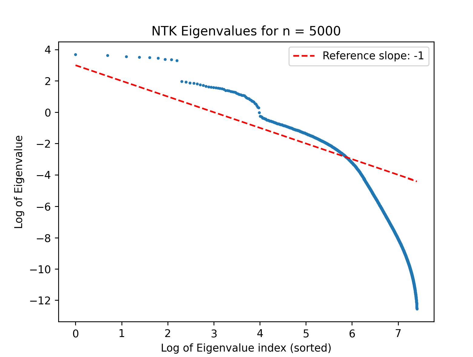
In Figure 2, we plot the natural logarithm of the sorted eigenvalues against the natural logarithm of their indices. The results show that the eigenvalues decay significantly faster than a reference line with slope , confirming that the decay rate is strictly greater than 1.
4.3 Classification on MNIST
4.3.1 Problem Formulation and Region Definition
We evaluated the efficacy of Mean Imputation (Dropout), Lazy Training, and Retraining methods for Variable Importance (VI) estimation using the MNIST dataset. The classification task was restricted to the digits ‘8’ and ‘9’, resulting in a training set size of approximately 11,800 images, with of this used as validation, and a test set of approximately 1,983 images. As illustrated in Figure 3, the primary structural distinction between these digits lies in the central-bottom region: the digit ‘8’ contains a closed loop crossing the midline, whereas the ‘9’ features a straight stroke or a curve that typically remains open in the center. Consequently, we hypothesized that the localized regions in the central-bottom area of the image (regions 10, 11, 14, and 15) would exhibit the highest variable importance. Conversely, we expected pixels in the upper regions (shared loop feature) and the far-left and far-right edges (typically empty background padding) to demonstrate negligible importance.
To mitigate the issue of high pixel-to-pixel correlation, where a single pixel’s value is highly predictive of its neighbors, we computed VI for groups of pixels rather than individual inputs. We analyzed the pixel images at three levels of granularity:
-
1.
Halves: Top vs. Bottom ( pixels).
-
2.
Quadrants: Four disjoint regions ( pixels).
-
3.
Fine-Grained Grid: Sixteen disjoint regions ( pixels).

4.3.2 Model Architecture and Implementation
We reused the same setup and architecture that controlled the Type I error in the Empirical Power study above. We implemented a feedforward neural network with two hidden layers, each containing 50 neurons with ReLU activation functions, and a final output layer producing logits for binary classification. The model was trained using the L-BFGS optimizer with a learning rate of . We used early stopping with a patience of 10 epochs to prevent overfitting, and the ridge penalty parameter was selected from a logarithmic path of 10 values ranging from to via 3-fold cross-validation.
For the VI comparisons, we defined the “Dropout” baseline as mean imputation, where pixels in a target region are replaced by their global mean intensity across the training set.
After training, we applied the LazyVI framework to assess the importance of each pixel region. We computed a one-sided -value for each region using the standard normal cumulative distribution function ():
where and denote the variable importance estimate and its standard error, respectively.
4.3.3 Results and Analysis
The comparative variable results are visualized in Figure 4. It is important to note that the color scale in the figure is normalized throughout the columns of a given row (granularity level) to facilitate comparison between methods, but not normalized across distinct rows.
Figure 5 shows a heatmap of the Lazy Training p-values for each region, adjusted with the Bonferroni correction. Each p-value was multiplied by 2, 4, or 16 for regions in the Top vs Bottom, Quadrant, and 16-Region granularities respectively, with the maximum adjusted p-value capped to 1. The plotted values are computed as . Note all p-values for the remainder of this section are reported with respect to the Bonferroni correction.


The results strongly support our central-bottom hypothesis and illustrate the value of fine-grained analysis. In the coarse-grained experiment, both halves were significant with , though the bottom half of the image was overwhelmingly dominant with a Lazy VI score of 0.1291 compared to 0.0338 for the top half. Once we moved to quadrants, we found the the three regions other than the Top-Left (TL) were significant, showing the significance of the top half was likely attributed to the Top-Right corner. In fact, this region had the largest VI estimate of the quadrants, unlike in Dropout and Retraining which had the Bottom-Left (BL) as the largest, which we attribute to randomness. The fine-grained analysis of the pixels revealed that the most important region was region 10 (), which physically corresponds to the closure of the bottom loop of the ‘8’ and its connection to the top loop, supporting our hypothesis.
The results strongly confirm our central-bottom hypothesis and illustrate the value of fine-grained analysis. In the coarse-grained experiments, the bottom half of the image was overwhelmingly dominant, yielding a Lazy VI score of 0.1291 () compared to 0.0046 () for the top half. Similarly, the quadrant analysis identified the Bottom-Left (BL) quadrant as the most critical, with a Lazy VI of 0.0360 () while the other quadrants were not statistically significant.
Finally, the fine-grained analysis revealed that this high "Bottom-Left" importance is likely driven almost entirely by the digit’s internal structure, as Region 10 was had variable importance of .0307 () while each other region in the Bottom-Left quadrant had p-values of 1. Physically, this region corresponds to the closure of the bottom loop of the ‘8’ and its connection to the top loop, which is absent in the typical ‘9’. Furthermore, all regions on an edge demonstrated -values of , with the exception of region 15 (), correctly identifying the empty background padding as uninformative.
Comparing the three estimation methodologies, we observed two key trends regarding magnitude and consistency:
-
1.
Magnitude Estimation and Overestimation: While the LazyVI framework closely matched the relative regional rankings predicted by Mean Imputation (Dropout), the magnitudes of LazyVI tracked the “ground truth” established by Retraining much more accurately. Dropout consistently overestimated Variable Importance, particularly when the dropped region was important. In the “Top vs Bottom” experiment, Dropout estimated the Bottom region’s importance at 1.050, which is approximately 14 times the “ground-truth” Retraining value of 0.075. Meanwhile, the Lazy Training estimate was 0.129, only 1.72 times the Retraining baseline. For the smaller, less important Region 10 subset of the bottom half, we observed an overestimation factor of times 4.10 for Dropout and 1.07 for Lazy Training of Retraining’s VI estimate of .029. In general, we noted that both Lazy Training and Dropout’s overestimation increases for more significant regions, but inflates disproportionately for Dropout while Lazy Training is minimally affected.
-
2.
Consistency Across Granularity: As the subset size decreased (from halves to squares), the estimated VI magnitudes decreased across all methods, as expected. However, the relative ranking between the regions remained consistent, and LazyVI successfully identified the main discriminative features with high fidelity—achieving results comparable to Retraining.
4.3.4 Runtime
In Table 2, we show the runtimes of training the full model, as well as Retraining and Lazy Training (not including the full model training time) for each region. Most of the time taken by Lazy Training is from the 30 trainings needed to choose a ridge penalty value, so for a more fair comparison, we showed the time taken for Lazy Training to run the final fitting. We found that the final fitting time for Lazy Training is consistently around 2 to 4 times faster than Retraining.
Because the runtime is dependent on the optimization techniques used, we expect the total runtime of Lazy Training could be optimized further. Warm starts for the final fitting using the solution from the cross-validation of the selected ridge penalty could speed up the final fitting time, but was excluded to make the comparison with Retraining fair. Warm starts during the cross-validation section and different optimizers such as Stochastic L-BFGS would also likely significantly improve runtime for the penalty selection process.
| Configuration | Region |
|
Retrain Time (s) | Full Model Time (s) | ||
| 16 Regions | 1 | 4.78 | 11.41 | 13.10 | ||
| 2 | 4.48 | 14.82 | ||||
| 3 | 4.56 | 15.10 | ||||
| 4 | 4.48 | 14.97 | ||||
| 5 | 4.55 | 12.03 | ||||
| 6 | 4.58 | 17.32 | ||||
| 7 | 4.55 | 15.31 | ||||
| 8 | 4.24 | 15.83 | ||||
| 9 | 4.54 | 12.38 | ||||
| 10 | 4.48 | 15.64 | ||||
| 11 | 4.55 | 14.82 | ||||
| 12 | 4.50 | 13.28 | ||||
| 13 | 4.53 | 12.01 | ||||
| 14 | 4.50 | 14.78 | ||||
| 15 | 4.51 | 17.23 | ||||
| 16 | 4.51 | 14.00 | ||||
| 4 Regions | TL | 4.64 | 18.84 | 12.81 | ||
| TR | 4.56 | 17.43 | ||||
| BL | 4.51 | 14.33 | ||||
| BR | 4.56 | 25.32 | ||||
| 2 Regions | Top | 4.62 | 19.37 | 13.08 | ||
| Bottom | 4.52 | 21.57 |
4.4 Application to Detect Genes Associated with Alzheimer’s Disease (AD)
Alzheimer’s disease (AD) is one of the most common neurodegenerative diseases, and it is influenced heavily through genetic components (Karch et al., 2014; Sims et al., 2020). Therefore, it is essential to detect genes significantly related to AD for targeted treatments. As an application of the proposed method, we performed a genetic association study based on the gene expression data from the Alzheimer’s Disease Neuroimaging Initiative (ADNI).
The disease status in the ADNI data has three categories: cognitive model, mild cognitive impairment, and Alzheimer’s disease. To apply our LazyVI for binary classification to the ADNI dataset, we combined mild cognitive impairment and Alzheimer’s disease into one group so that the classifier can detect genes that potentially relate to any potential neural degeneration. We then merged data from individuals having both gene expression information and disease status. A total of 521 individuals and 15,837 gene expressions were obtained.
We then performed a variable importance test for each of the 15,837 gene expression variables. In other words, we conducted 15,837 hypothesis tests, where the null hypothesis states that the gene is not important and the alternative hypothesis states that the gene is important. To fit the model under the alternative hypothesis, we included age, gender, years of education, the number of APOE4 alleles, and the expression level of the gene of interest as input features. Under the null hypothesis, we replaced the gene expression level with its sample mean and applied our LazyVI algorithm. Following the simulation setup, we fitted the data using a deep ReLU network (two hidden layers, 50 neurons per layer). The regularization parameter and the hyperparameters in the L-BFGS algorithm were kept identical to those used in the simulation studies. After obtaining the -values for all genes, we ranked them from smallest to largest. Table 3 summarizes the 10 most significant genes identified by logistic regression and the LazyVI algorithm.
| Logistic Regression | LazyVI |
| ORC6 | MT1H |
| SPATA7 | COMMD6 |
| GPAT2 | LRFN3 |
| OR52B2 | GLRX5 |
| KRTAP6-3 | SGCB |
| TAS2R10 | TCF19 |
| SLITRK6 | NKX2-6 |
| ZNF503 | PIGC |
| KCTD8 | PSTPIP1 |
| OR52A5 | MAPK11 |
It is not surprising that deep neural network-based methods identify different genes from those identified by classical statistical methods. For instance, Shen and Wang (2024) applied a goodness-of-fit test based on deep ReLU neural networks to detect genes associated with quantitative traits related to AD, and the genes identified by the deep neural network-based methods differed substantially from those identified by linear models. On the other hand, it is worth noting that the most significant genes identified by each method have biological relevance supported by previous studies. The origin recognition complex (ORC), which controls the initiation of DNA replication, consists of six subunits, one of which is ORC6. Arendt and Brückner (2007) showed that ORC subunits are involved in AD pathology. Among the significant genes identified by the LazyVI algorithm, MT1H, which belongs to the metallothionein family, has been uncovered as a hub gene through a network analysis and is suspected to be related to AD development for long time (Liang et al., 2018). In addition, MAPK11 is a member of the mitogen-activated protein kinase (MAPK) family. As mentioned in Zhao et al. (2002), the MAPK family regulates phosphorylation of the microtubule-associated protein tau and processing of the amyloid protein , and both events are critical to the pathophysiology of AD. These findings suggest that our method successfully identifies genes involved in biological pathways known to contribute to AD pathogenesis while also revealing potentially novel candidate genes for future investigation.
5 Discussions and Conclusions
In this paper, we propose a framework for detecting important input features using lazy-trained deep neural network features in binary classification problems. We rigorously establish the asymptotic normality of the proposed test statistics. Through simulation studies and experiments on the MNIST dataset, the LazyVI framework successfully identifies important features. Moreover, compared with dropout-based methods, LazyVI generally does not overestimate variable importance scores. At the same time, the variable importance scores estimated by LazyVI are approximately the same as those obtained from retraining-based methods. Nevertheless, LazyVI is computationally more efficient than retraining-based approaches.
The universal approximation property of neural networks (Hornik et al., 1989; Cybenko, 1989; Yarotsky, 2017; Yarotsky and Zhevnerchuk, 2020; Schmidt-Hieber, 2020) provides a powerful alternative for function estimation in nonparametric statistical models (e.g., nonparametric regression). However, conducting statistical inference based on a fitted neural network for the purpose of detecting important input features remains a challenging problem. Although the proposed LazyVI framework primarily focuses on binary classification, we believe it has the potential to be extended to other types of outcome variables. A natural generalization is to replace the binary cross-entropy loss with the multiclass cross-entropy loss, thereby accommodating multiclass classification problems. Indeed, we formulate the problem using a Bernoulli distribution in Section 3.1 to connect our framework with the classical formulation of generalized linear models (GLMs) (McCullagh and Nelder, 1999), where the conditional distribution of is typically assumed to belong to the exponential dispersion family:
where is the dispersion parameter and , , and are known functions. The relationship between and is specified through a link function such that
| (31) |
The linear predictor can be naturally generalized to a nonlinear function by replacing it in (31). Consequently, within the framework described in Section 3.1, we may define the loss function as the negative log-likelihood
If this loss function satisfies Conditions 1–3 in Proposition 10, then the LazyVI framework can be applied in this more general setting.
We would also like to highlight several limitations of the current method. (1) In this paper, we focus primarily on the function class of fully connected deep neural networks. It would be worthwhile to investigate whether the framework can be extended to more sophisticated architectures, including convolutional neural networks (LeCun, 1989), long short-term memory networks (Hochreiter and Schmidhuber, 1997), and transformers with attention mechanisms (Vaswani et al., 2017). (2) As indicated by Assumption (16), our analysis primarily considers the regime in which the number of network parameters does not grow too rapidly relative to the sample size. However, due to the empirical success of large-scale deep learning models, overparameterized neural networks have attracted substantial attention in recent years. It is therefore important to investigate whether the LazyVI framework can be extended to the overparameterized setting. For the framework developed in this paper, the main technical bottleneck underlying these two limitations concerns whether a sufficiently tight upper bound on the entropy numbers of the function class can be established and how this bound scales with the covering radius . The volume-based argument we employ yields a growth rate of order , but at the cost of dependence on the total number of network parameters. This dependence ultimately affects the convergence rate derived via local Rademacher complexity arguments. In contrast, applying Maurey’s sparsification lemma (Pisier, 1981) yields size-independent upper bounds on entropy numbers; however, the resulting growth rate is of order , as shown in Zhang (2004) and Bartlett et al. (2017). Moreover, Golowich et al. (2018) demonstrate that the Rademacher complexity of neural networks with parameter matrices of bounded Schatten norm is lower bounded by , which makes it challenging to derive faster convergence rates even when using local Rademacher complexity. (3) Although, in theory, Newton’s method can be used to compute the estimators arising from the lazy training procedure, this becomes computationally prohibitive for very large sample sizes, since the neural tangent kernel matrix has dimension . For example, the UK Biobank dataset (Bycroft et al., 2018) contains over 500,000 participants. Storing such large matrices requires substantial memory, and inverting the corresponding Hessian matrices further increases the computational burden. In our implementation, we therefore adopt a quasi-Newton method to reduce computational cost. Nevertheless, applying the LazyVI framework to large-scale datasets such as UK Biobank requires the development of more scalable algorithms. Addressing these limitations will be the focus of future work.
To conclude, our work demonstrates that statistically valid inference for feature importance can be carried out in deep neural networks by leveraging the lazy training regime and likelihood-based formulations. By connecting neural tangent kernel approximations with classical tools from empirical process theory and generalized linear models, our framework provides a principled bridge between deep neural networks and traditional statistical inference. We hope this perspective encourages further research on scalable and theoretically grounded inference procedures for deep learning models beyond predictive performance alone.
Software and Appendices
The proposed LazyVI framework for detecting important features for binary classification was implemented using Python packages. The codes and simulated data are available at https://github.com/SxxMichael/DNN-LazyVI-Binary-Classification. Additional technical details are available in the Appendices.
Acknowledgements
This research is supported in part by NSF Grant DMS-2447229.
References
- Linking cell-cycle dysfunction in alzheimer’s disease to a failure of synaptic plasticity. Biochimica et Biophysica Acta (BBA)-Molecular Basis of Disease 1772 (4), pp. 413–421. Cited by: §4.4.
- Theory of reproducing kernels. Transactions of the American mathematical society 68 (3), pp. 337–404. Cited by: §2.1.
- Spectrally-normalized margin bounds for neural networks. Advances in neural information processing systems 30. Cited by: §3.1, §5.
- Rademacher and gaussian complexities: risk bounds and structural results. Journal of machine learning research 3 (Nov), pp. 463–482. Cited by: §E.2, Remark 29.
- Local Rademacher complexities. The Annals of Statistics 33 (4), pp. 1497 – 1537. Cited by: §E.1, §E.1, §E.1, §E.2, §E.2, §E.2, §F.4, §2.2, §2.2, §3.3, Lemma 5, Theorem 6.
- Deep equals shallow for relu networks in kernel regimes. arXiv preprint arXiv:2009.14397. Cited by: §3.2.
- On the inductive bias of neural tangent kernels. Advances in Neural Information Processing Systems 32. Cited by: §3.2.
- The uk biobank resource with deep phenotyping and genomic data. Nature 562 (7726), pp. 203–209. Cited by: §5.
- On lazy training in differentiable programming. Advances in neural information processing systems 32. Cited by: §1.1.
- Approximation by superpositions of a sigmoidal function. Mathematics of control, signals and systems 2 (4), pp. 303–314. Cited by: §5.
- Significance tests of feature relevance for a black-box learner. IEEE transactions on neural networks and learning systems 35 (2), pp. 1898–1911. Cited by: §1.1, §4.1.3.
- Gradient descent provably optimizes over-parameterized neural networks. arXiv preprint arXiv:1810.02054. Cited by: §3.2.
- Deep neural networks for estimation and inference. Econometrica 89 (1), pp. 181–213. Cited by: §B.2, §3.3.
- Lazy estimation of variable importance for large neural networks. In International Conference on Machine Learning, pp. 7122–7143. Cited by: 2nd item, 2nd item, §1.1, §3.2, §3.5.
- Size-independent sample complexity of neural networks. In Conference on learning theory, pp. 297–299. Cited by: §5.
- Long short-term memory. Neural computation 9 (8), pp. 1735–1780. Cited by: §5.
- Probability inequalities for sums of bounded random variables. The collected works of Wassily Hoeffding, pp. 409–426. Cited by: 5th item.
- Significance tests for neural networks. Journal of Machine Learning Research 21 (227), pp. 1–29. Cited by: §1.1.
- Multilayer feedforward networks are universal approximators. Neural networks 2 (5), pp. 359–366. Cited by: §5.
- A tail inequality for quadratic forms of subgaussian random vectors. Electronic Communications in Probability 17, pp. 1–6. Cited by: §C.2, §C.2, 5th item, 2nd item.
- Neural tangent kernel: convergence and generalization in neural networks. Advances in neural information processing systems 31. Cited by: §3.1.
- Alzheimer’s disease genetics: from the bench to the clinic. Neuron 83 (1), pp. 11–26. Cited by: §4.4.
- Gradient-based learning applied to document recognition. Proceedings of the IEEE 86 (11), pp. 2278–2324. Cited by: §4.
- Generalization and network design strategies. Connectionism in perspective, pp. 143–155. Cited by: §5.
- Probability in banach spaces: isoperimetry and processes. Springer Science & Business Media. Cited by: §E.1, §E.1, §E.2.
- On the eigenvalue decay rates of a class of neural-network related kernel functions defined on general domains. Journal of Machine Learning Research 25 (82), pp. 1–47. Cited by: §3.2.
- Application of weighted gene co-expression network analysis to explore the key genes in alzheimer’s disease. Journal of Alzheimer’s Disease 65 (4), pp. 1353–1364. Cited by: §4.4.
- A unified approach to interpreting model predictions. Advances in neural information processing systems 30. Cited by: §1.1.
- Lecture notes for machine learning theory (cs229m/stats214). Cited by: §B.2.
- Permutation-based hypothesis testing for neural networks. In Proceedings of the AAAI Conference on Artificial Intelligence, Vol. 38, pp. 14306–14314. Cited by: §1.1.
- Generalized linear models. Chapman & Hall/CRC. Cited by: 1st item, §5.
- Improving the sample complexity using global data. IEEE transactions on Information Theory 48 (7), pp. 1977–1991. Cited by: §F.3.
- A trace inequality of john von neumann. Monatshefte für mathematik 79 (4), pp. 303–306. Cited by: 5th item.
- Six lectures on linearized neural networks. Journal of Statistical Mechanics: Theory and Experiment 2024 (10), pp. 104006. Cited by: §C.3, §3.4.
- Foundations of machine learning. MIT press. Cited by: §2.2.
- Rectified linear units improve restricted boltzmann machines. In Proceedings of the 27th international conference on machine learning (ICML-10), pp. 807–814. Cited by: §3.1.
- Numerical optimization. Springer Series in Operations Research. Cited by: 1st item, footnote 1.
- A central limit theorem under metric entropy with l 2 bracketing. The Annals of Probability, pp. 897–919. Cited by: §E.3.
- Toward moderate overparameterization: global convergence guarantees for training shallow neural networks. IEEE Journal on Selected Areas in Information Theory 1 (1), pp. 84–105. Cited by: §3.2, §3.4.
- Rise: randomized input sampling for explanation of black-box models. arXiv preprint arXiv:1806.07421. Cited by: §1.1.
- Remarques sur un résultat non publié de b. maurey. Séminaire d’Analyse fonctionnelle (dit" Maurey-Schwartz"), pp. 1–12. Cited by: §5.
- Nonparametric regression using deep neural networks with relu activation function. The Annals of Statistics 48 (4). Cited by: §3.3, §5.
- Consistency and rate of convergence for deep relu neural networks. Journal of Statistical Theory and Practice 19 (2), pp. 33. Cited by: §3.3.
- A goodness-of-fit test based on neural network sieve estimators. Statistics & probability letters 174, pp. 109100. Cited by: §1.1.
- A sieve quasi-likelihood ratio test for neural networks with applications to genetic association studies. arXiv preprint arXiv:2212.08255. Cited by: §1.1.
- Asymptotic properties of neural network sieve estimators. Journal of nonparametric statistics 35 (4), pp. 839–868. Cited by: §3.3.
- An exploration of testing genetic associations using goodness-of-fit statistics based on deep relu neural networks. Frontiers in Systems Biology 4, pp. 1460369. Cited by: §1.1, §4.4.
- Deep inside convolutional networks: visualising image classification models and saliency maps. arXiv preprint arXiv:1312.6034. Cited by: §1.1.
- The multiplex model of the genetics of alzheimer’s disease. Nature neuroscience 23 (3), pp. 311–322. Cited by: §4.4.
- Smoothgrad: removing noise by adding noise. arXiv preprint arXiv:1706.03825. Cited by: §1.1.
- Weak convergence and empirical processes: with applications to statisticsWeak convergence and empirical processes: with applications to statistics. Springer. Cited by: §E.3.
- Attention is all you need. Advances in neural information processing systems 30. Cited by: §5.
- High-dimensional probability: an introduction with applications in data science. Cambridge University Press. Cited by: §B.2, §F.5.
- A general framework for inference on algorithm-agnostic variable importance. Journal of the American Statistical Association 118 (543), pp. 1645–1658. Cited by: 2nd item, §1.1, §2.3, §2.3, §3.6, Theorem 7.
- The phase diagram of approximation rates for deep neural networks. Advances in neural information processing systems 33, pp. 13005–13015. Cited by: §5.
- Error bounds for approximations with deep relu networks. Neural networks 94, pp. 103–114. Cited by: §5.
- Towards unified attribution in explainable ai, data-centric ai, and mechanistic interpretability. External Links: 2501.18887, Link Cited by: §1.1.
- Statistical analysis of some multi-category large margin classification methods. Journal of Machine Learning Research 5 (Oct), pp. 1225–1251. Cited by: §5.
- MAP kinase signaling cascade dysfunction specific to alzheimer’s disease in fibroblasts. Neurobiology of disease 11 (1), pp. 166–183. Cited by: §4.4.
- Stochastic gradient descent optimizes over-parameterized deep relu networks. arXiv preprint arXiv:1811.08888. Cited by: §3.4.
Appendix
In this appendix, we provide detailed proofs of the results in the main text. We organize the appendix as follows:
Appendix A Properties for 0-1 Logistic Loss
A.1 Proof of Proposition 8
Proof.
Let and with being the sigmoid function. Here represents the underlying conditional distribution of and represents the estimated conditional distribution of based on our model. Then the KL divergence between these two distributions is
where does not depend on . Therefore,
Since , then under the assumption that , the minimum is attained when , -almost surely. Consequently, the minimum is attained when and hence if is a minimizer, then , -almost surely. ∎
A.2 Proof of Proposition 10
Proof.
-
1.
Note that
and since is non-negative for all , it follows that is convex with respect to .
-
2.
Since and for all , it then follows that for all . Based on the mean value theorem, for any , there exists between and such that
As a result, for any ,
-
3.
Let be arbitrary such that . Now consider the Taylor expansion of and around the mid-point .
where is between and and is between and . Then
Since and is an even function that is monotonically decreasing when , it then follows that
Hence
∎
A.3 Proof of Corollary 11
Proof.
For any and satisfying , we have
where (*) and (**) follow from the definition and the lower bound of the modulus of convexity in (15). Therefore, we obtain a lower bound for the modulus of convexity for :
which implies that
where the 2nd inequality follows from the fact that minimizes . Hence,
Rearranging the above display yields the desired result. ∎
Appendix B Technical Results for Deep ReLU Neural Networks
B.1 Proof of Lemma 13
Proof.
It is easy to see that is a 1-Lipschitz function so that for any and ,
Consequently, for any ,
∎
B.2 Proof of Lemma 14
The proof relies on bounding the covering number of . To do this, we applied the following result (Lemma 5.23) from Ma (2022).
Lemma 26.
Let be a function class such that
Assume
-
1.
is -Lipschitz, that is
-
2.
The Euclidean norm of every input to is bounded by .
-
3.
The metric entropy of is bounded as follow:
Then there exists an -cover of for such that
For the class of deep ReLU neural network as described in (8), we can set
It is obvious that each , is a -Lipschitz function. In terms of the Euclidean norm of the inputs, we have
| (32) |
where . In addition, let . Suppose that is a minimal cover of with respect to . Then for any , we have for some and there exists such that
Then set , we have
where is the input of the the layer in the network for the th sample. Then
Now note that for any ,
Then by Proposition 4.2.12 in Vershynin (2018), we have
and hence
| (33) |
Based on these observations, we are now ready to prove Lemma 14.
Proof.
Denote and take
| (34) |
Then
In addition,
It then follows from Lemma 26 and (33) that
Recall that . Now based on Lemma 32, it follows that
For any , we have for some and , it then follows that
Therefore, it suffices to consider . In this case, since for all , we have
which implies that
| (35) |
Next, by the Dudley’s chaining technique (see for example, Lemma 3 in Farrell et al. (2021)) that
For notation simplicity, denote . According to (35), we have
where the last inequality follows since so that .
As a result,
We now show that is a sub-root function. To do so, we check the three conditions required for a function to be sub-root.
-
1.
First note that , then , which immediately shows that is nonnegative.
-
2.
Note that
where the last inequality follows since and hence . Hence, is a nondecreasing function.
-
3.
Since , it is obvious that is nonincreasing.
We now provide an upper bound for the fixed point of . Note that
which implies that and hence,
Therefore,
∎
B.3 Proof of Theorem 15
Proof.
To start with, we check the conditions required in Theorem 12. Condition 1 holds immediately based on our assumption . Conditions 2 and 3 follow from Proposition 10 with and . In addition, note that
Therefore, it follows from Theorem 12 by taking that with probability at least ,
where the 2nd inequality follows since and
∎
B.4 Proof of Corollary 16
Proof.
Using the notations in Theorem 9, it is easy to see that . It then follows from Lemma 14 that
Let and . Note that for any , , so without loss of generality, we may assume and it follows from the same reasoning as in the proof of Lemma 14 that is a sub-root function with fixed point
In view of Lemma 33, we can know that the fixed point of is bounded by
Therefore, by Theorem 9, with probability at least ,
Consequently,
∎
Appendix C Distance Between Linearized Deep ReLU Network and the Deep ReLU Network
C.1 Proof of Lemma 17
Proof.
Note that
where the last inequality follows since based on the definition of . Similarly, for ,
where the inequality (*) follows from (32) and . Consequently,
The desired result then follows by applying the inequality for positive .
For the bound on , note that
∎
C.2 Proof of Proposition 18
Proof.
We first prove the result for . Since is a convex function, the Newton-Raphson algorithm is guaranteed to converge to its minimum. Therefore, needs to satisfy
| (36) |
which implies that needs to satisfy
| (37) |
Therefore, by the triangle inequality,
Since elements in are independent, mean-zero sub-Gaussian random variables, it follows from Theorem 1 in Hsu et al. (2012) that with probability at least ,
Note that , then with probability at least ,
Hence, with probability at least ,
For the second term, note that by the mean value theorem,
| (38) |
where with some . Since , we have with probability at least ,
| (39) |
where the last equality follows since . Therefore, by rearranging (41), we have
Based on (A2), we have
| (40) |
In addition, note that , we have
Therefore, under assumption (A2), combined with Corollary 16, with probability at least ,
We now prove the result for . Based on (37) and triangle inequality,
Since elements in are independent, mean-zero sub-Gaussian random variables, it follows from Theorem 1 in Hsu et al. (2012) that with probability at least ,
Note that
then with probability at least ,
Hence, with probability at least ,
For the second term, by (38) we have with probability at least ,
| (41) |
where the last inequality follows from Lemma 17. Therefore, by rearranging (41), we have
Since and as , based on (40), we have
Combine everything together, we have under assumption (A2), with probability at least ,
∎
C.3 Proof of Theorem 19
Proof.
Applying Taylor’s theorem similar to equation (1.3.2) in Misiakiewicz and Montanari (2024), we have
where the last two inequalities follow from the Cauchy-Schwarz inequality and the triangle inequality. According to Lemma 17, the norms of the gradient are upper bounded by . Therefore, for any satisfying ,
Denote , and . Then from Proposition 18, we know that
Let . Given , take , then and . Therefore, for , , and hence
Since , , , and , we have
which implies that
∎
Appendix D Technical Details on the Convergence Rate of Linearized ReLU Network
D.1 Proof of Lemma 20
Proof.
Denote . First note that
where (1), (2), and (5) hold from the triangle inequality, (3) comes from the definition of the operator norm, and (4) follows from Lemma 31. We now provide bounds for each term.
-
•
Bound for . We derive the bound for by iterating Newton’s updating equation times. Nocedal and Wright (2006)111Theorem(Nocedal and Wright, 2006) Suppose that f is twice differentiable, that the Hessian is Lipschitz continuous, and that and is positive definite. Consider the iteration . Then (1) if the starting point is sufficiently close to , the sequence of iterates converges to and (2) the rate of convergence of is quadratic, i.e., there exists some constant such that for . shows that when the target function is twice differentiable and the Hessian is Lipschitz continuous and positive definite, the rate of convergence of Newton’s method is quadratic. Since is clearly twice differentiable and the Hesssian is positive definite due to is positive semidefinite. On the other hand, the Hessian is also Lipschitz continuous by noting that
where (1) follows from the Lipschitz continuity of and (2) follows from the Rayleigh quotient property of symmetric matrices. Notice does not depend on , proving the Hessian is Lipschitz. Thus, we know that . Since as , there exists such that . Therefore for all , combining the assumption (A2) with Proposition 18, we have
-
•
Bound for . Recall that
so then
Note that for any , we have
so the reciprocal
Therefore,
where
Since functions in are uniformly bounded by , we have
Then
where (1) holds by Cauchy–Schwarz and (2) holds from Lemma 17 and the bound for . So,
Therefore
(42) -
•
Bound for . We have the following bound on :
Using the bound for and the bound on , we have
-
•
Bound for . Since , it then follows from the Corollary 16 that with probability at least , .
-
•
Bound for . Note that and , it then follows that . By Hoeffding inequality (Hoeffding, 1994),
which implies , are sub-Gaussian random variables with sub-Gaussian parameter 1. Therefore, for any ,
By Theorem 1 in Hsu et al. (2012), for any ,
where . Note that
In addition, we have
where (a), (b) and (d) follow from the von Neumann trace inequality (Mirsky, 1975); (c) follows from the AM-GM inequality and (e) follows since is a diagonal matrix and the largest diagonal element is bounded by 1.
Combining these two observations together, we have
Therefore, for any , with probability at least ,
where (*) holds from the bound for and Lemma 17; (**) holds from the Assumption (A2) that .
Putting all the pieces together, we have with probability at least ,
which proves (19). Equation (20) now follows immediately from Proposition 18. ∎
D.2 Proof of Lemma 21
Proof.
Recall that and denote . Then and
where (*) follows by noting that
and is clearly a positive semidefinite matrix. Additionally, (**) follows from the triangle inequality based on the norm with being a positive semidefinite matrix. We now bound and .
- •
- •
Putting all the pieces together with the assumption (A2), we have with probability at least ,
which proves (21) and (22) follows by applying the upper bound for given in Proposition 18. ∎
D.3 Proof of Lemma 22
Proof.
We prove this result by applying Theorem 9. Using the notation in Theorem 9, we let and . Then for any satisfying , we know that there exists and such that
which implies that
On the other hand, note that is star-shaped around 0, we know that . Therefore,
which implies that
Hence the desired result follows from Theorem 9. ∎
D.4 Proof of Lemma 23
Proof.
For notation simplicity, denote . Let be such that and . Then for all . Then
Then since
Let and we have shown that
Now take
Now let us claim that is a sub-root function. It is obvious that is nonnegative and nondecreasing since . So it suffices to show that is nonincreasing. But note that
and since both and are decreasing functions in , it follows that is nonincreasing for . On the other hand, let . In view of Lemma 33, we have , where and represent the fixed points of and respectively. Therefore, it suffices to find . Let and note that
and solving gives
which implies that . Putting all the pieces together,
∎
D.5 Proof of Theorem 24
Proof.
We first prove (26). Recall that . By Lemma 30,
Based on Lemma 21, with probability at least ,
On the other hand, based on Lemma 17,
Therefore, with probability at least ,
| (43) |
Then by combining Lemma 20, Lemma 22 and Lemma 23, we have with probability at least ,
where the inequality (*) follows since
| (44) | ||||
| (45) |
Appendix E Proof of the Main Results
E.1 Proof of Theorem 9
Proof.
Define
| (46) |
Fix . Let and . Additionally, let us define a functional as
Since functions in are uniformly bounded by 1, we have for any ,
| (47) |
According to (47), the property that the functional needs to satisfy in order to apply Theorem 6 is satisfied with . Therefore, with probability at least , for any ,
| (48) | ||||
| (49) |
where is the fixed point for some sub-root function . In addition, note that
where the last inequality follows from the Ledoux-Talagrand contraction principle (Ledoux and Talagrand, 2013). Therefore, it suffices to find a sub-root function that upper bounds .
To do this, note that for , there exists such that
On the other hand, it follows from (47) and Theorem 2.1 in Bartlett et al. (2005) (with the choice of ) that with probability at least ,
where (*) follows from the AM-GM inequality:
(**) follows from the Ledoux-Talagrand contraction principle (Ledoux and Talagrand, 2013) and the last inequality follows since
Denote
It then follows from Lemma 5 that is a sub-root function. Therefore, we have for all ,
In addition, if satisfies , then with probability at least ,
Consequently, if , with probability at least ,
On the other hand, by Lemma A.4 in Bartlett et al. (2005), with probability at least ,
| (50) |
Then if , with probability at least ,
Based on our assumption, , we have with probability at least ,
| (51) |
Then by Lemma 4.3 in Bartlett et al. (2005), with probability at least , . Putting (51) and (49), (48) together, with probability at least , for any ,
which is equivalent to (recall that ),
The desired result then follows by using the elementary inequality for . ∎
E.2 Proof of Theorem 12
To prove the theorem, we start by proving a preparatory lemma:
Lemma 27.
Proof.
For simplicity, denote and let . For any , define
Then by the condition 2 and 3 in the lemma,
On the other hand, by the contraction principle (Ledoux and Talagrand, 2013),
Hence, by the assumption on ,
Since , it then follows from Theorem 6 that for any , with probability at least ,
where is the fixed point of . Replace by and note that since is the minimizer of . Hence, with probability at least
Finally, by Lemma 3.2 in Bartlett et al. (2005) that is equivalent to , which leads to the desired result. ∎
We are now ready to prove the theorem.
Proof.
Define
where . It is easy to see that for any . Since , we have
In addition, according to Lemma 5 with the choice of that is subroot. Now for , Lemma 27 and condition 3 on the loss function imply that for any , with probability at least ,
| (52) |
On the other hand, for , by the definition of and , we have.
Then by Corollary 2.2 in Bartlett et al. (2005), with probability at least ,
Combined with Lemma A.4 in Bartlett and Mendelson (2002), with probability at least ,
Setting , the fixed point of in the above argument and applying Lemma 4.3 in Bartlett et al. (2005) shows that , which together with (52) concludes the proof. ∎
E.3 Proof of Theorem 25
Proof.
In view of Theorem 7, it suffices to check the required conditions.
-
Condition (D1). By the first order Taylor expansion of with respect to ,
where for some and (*) follows since from Proposition 8.
-
Condition (D2). For any and satisfying and , by (29),
-
Condition (R3). As we have seen above, , let us define
So it is obvious that , -a.s. In view of Theorem 3.1 in Ossiander (1987), to show that is a -Donsker class, it suffice to show that
On the other hand, since , where the last inequality follows from the relationship between covering number and bracketing number mentioned in Van Der Vaart and Wellner (1996), we have
Now, let be a minimal -cover of with respect to the uniform norm . Then and for any , there exists such that . Denote
Then for any , by the Lipschitz continuity of , we have
which implies that
It then follows from Theorem 36 that
where in the first inequality, we can change the upper bound of the entropy integral to since functions in are uniformly bounded by and the finiteness of the entropy integral follows by a similar argument as in the proof of Lemma 14. Hence, is a -Donsker class.
∎
Appendix F Auxiliary Results
F.1 The RKHS Associated with the NTK
In this section, we provide the detailed proofs of the results on the RKHS generated by the NTK.
Lemma 28 (Local Rademacher Complexity of ).
where are the eigenvalues of arranged in a decreasing order.
Proof.
Note that
Let be the spectral decomposition of with and denote . Then
Therefore,
where . Let , it then follows from Cauchy-Schwarz inequality that
where (*) follows from Jensen’s inequality and . ∎
Remark 29.
Lemma 30 (Uniform Boundedness of Functions in ).
For any ,
Proof.
For any , there exists such that . Then by Cauchy-Schwarz inequality,
Therefore, for any
∎
F.2 Lipschitzness of Sigmoid Function
Lemma 31.
For any two vectors , we have
Proof.
By Lipschitz continuity of the sigmoid function, we know that for any , the following is true:
Thus, for any 2 vectors ,
Taking the square root yields
∎
F.3 Covering Number of the Star Hull of a Function Class
The following lemma is similar to Lemma 4.5 in Mendelson (2002), which shows that the covering number of the star hull of a function class is almost the same as the covering number of .
Lemma 32.
Suppose that is a class of functions with ranges in and be a fixed function. Then for any pseudo-norm ,
Proof.
Fix . Let be a minimal -cover of . Then . In addition, define
For any , there exists and such that . For such a function , there exists such that . Denote
which implies that
On the other hand, let be a minimal -cover of so that there exists such that
As a result, we have
This shows that is a -cover of and hence
Note that for each , we have . Now consider the partition of with breakpoints , . For any , there exists such that . Based on the construction of partition, there exists such that . As a result
which implies that . Hence,
Taking logarithm on both sides yields the desired result. ∎
F.4 Fixed Points of Adding a Constant to Sub-root Functions
Lemma 33.
Let be a sub-root function and let be a constant. Define
and let be the fixed points of and respectively. Then
Proof.
By the definition of , we have
it then follows from Lemma 3.2 in Bartlett et al. (2005) that . On the other hand, since is non-increasing, we have
which implies that
Squaring both sides of the above inequality yields
and solving this inequality with respect to , we have
∎
F.5 Covering Number of Deep ReLU Network Under the -norm
Lemma 34.
Let for some and let be a 1-Lipschitz function. Define
| (55) |
where and
for some . Denote . Then
Here .
Proof.
Lemma 35.
Let be a class of functions and let be a class of -Lipschitz function. Define
Then
Proof.
For any , there exists and such that . Let be a minimal -cover of so that and let be a minimal -cover of so that . Then there exists such that
and there exists such that
Consequently,
For the first term, by the Lipschitz continuity of ,
For the second term, we have
Therefore, forms an -cover for and the desired result follows. ∎
Theorem 36.
Let be the class of deep ReLU neural networks as defined in (8). Then