Weighted Extensions of the Kolmogorov–Smirnov, Cramér–von Mises, and Anderson–Darling Tests for Assessing Covariate Balance
Abstract
Assessing covariate balance is a core diagnostic step in causal inference, but commonly used summary measures can miss meaningful distributional differences they are not designed to detect. Distributional goodness-of-fit tests, including the Kolmogorov–Smirnov (KS), Anderson–Darling (AD), and Cramér–von Mises (CVM) tests, offer a more complete comparison but have previously been available only for unweighted data. We extend all three to accommodate case weights of any origin, using a shared label-permutation inference procedure that requires no assumption about how the weights were generated. In a four-scenario simulation study, all three weighted tests controlled Type I error close to nominal across sample sizes from 1,000 to 4,000 under substantial weight variability. Each test’s known unweighted comparative advantage was preserved under weighting for two of three discrepancy types: KS was most powerful against a centrally located discrepancy, and AD was overwhelmingly most powerful against a tail-located discrepancy, while AD and CVM performed comparably against a diffuse discrepancy, both outperforming KS. These findings support AD as a reasonable general-purpose default for routine covariate-balance assessment, while KS retains an advantage when a centrally concentrated imbalance is specifically suspected. The methods are implemented in the Stata commands kstest, adtest, and cvmtest.
Keywords
covariate balance; distributional tests; Kolmogorov–Smirnov test; Anderson–Darling test; Cramér–von Mises test; permutation inference; weighting
1 Introduction
Balance testing is an integral component of causal inferential methods. Covariate balance may be achieved by design, as in randomized experiments, or by post-hoc adjustment, as in propensity-score weighting, matching, or stratification. Either way, demonstrating that treated and comparison groups are comparable on observed, measured characteristics is a necessary step in supporting a causal interpretation of an estimated treatment effect (Rubin,, 2008). This step rests on the assumption that any remaining differences in unmeasured characteristics are not large enough to meaningfully confound the results. Balance testing on measured covariates is the closest empirical check available on that assumption, even though it cannot verify it directly (Rubin,, 1973).
In applied practice, covariate balance is most commonly assessed using summary measures such as the standardized mean difference and the variance ratio between groups (Austin,, 2009, 2015; Stuart,, 2010; Linden and Samuels,, 2013). Some recent additional measures include the Somer’s D statistic, a nonparametric measure of ordinal association (Newson and Falcaro,, 2023), and the optimal discriminant analysis cutpoint, a machine learning method (Linden and Yarnold,, 2016). These measures are simple to compute and report, but they share a common limitation: each targets only a specific point in a covariate’s distribution. Two distributions can share an identical value at that point while differing substantially elsewhere, for example in their skewness, in the location of their mass, or in their tails. By construction, these measures of balance are unable to detect such differences.
Goodness-of-fit tests based on the empirical cumulative distribution function (ECDF) offer a more complete alternative, comparing the entire distributions of a covariate across groups rather than a small number of summary moments. Three such tests are well established for this purpose: the Kolmogorov–Smirnov (KS) (Kolmogorov,, 1933; Smirnov,, 1948), Anderson–Darling (AD) (Anderson and Darling,, 1952), and Cramér–von Mises (CVM) (Cramér,, 1928; von Mises,, 1931) tests. Until now, however, all three have been available only for unweighted data. This has limited their use in exactly the setting where distributional balance is most often of interest: after inverse probability of treatment weighting (Robins et al.,, 2000), entropy balancing (Hainmueller,, 2012), marginal mean weighting through stratification (Linden,, 2014), classification tree endpoint weights (Linden and Yarnold,, 2017, 2018), or other case-weighting adjustments intended to equate treated and comparison groups. This paper makes two contributions. First, we extend all three tests to accommodate case weights of any origin, making them available as an additional tool for covariate balance assessment in weighted analyses. Second, we develop a single label-permutation inference procedure that treats an observation’s weight as a fixed, given attribute rather than a quantity tied to a specific estimation method. Because this procedure makes no assumption about how a given weight was generated, it applies without modification to any weighting scheme a user might supply. The methods are implemented in the community-contributed Stata commands kstest (Linden,, 2026), adtest (Linden, 2025a, ), and cvmtest (Linden, 2025b, ).
The three tests are not interchangeable, however. In their unweighted form, they are known to differ systematically in their sensitivity to where a distributional discrepancy is located. This property follows directly from each statistic’s construction and is well documented in the classical, unweighted goodness-of-fit literature (Stephens,, 1974; D’Agostino and Stephens,, 1986). The Kolmogorov–Smirnov statistic is determined entirely by the single point of greatest divergence between the two distributions, discarding information about any other point at which the distributions may differ. It is therefore best suited to detecting a discrepancy that is large and localized, wherever it occurs, but can be insensitive to multiple, smaller discrepancies elsewhere in the distribution. The Cramér–von Mises statistic imposes no variance standardization, summing squared discrepancies uniformly across the full support of the distribution. It is consequently best suited to detecting discrepancies that are diffuse across the distribution rather than concentrated in either the tails or a single location. The Anderson–Darling statistic’s variance-standardization term is smallest at the center of the pooled distribution and largest near its tails, giving it disproportionate sensitivity to discrepancies located in the tails relative to discrepancies of the same magnitude located centrally.
In this study, we examine, via simulation, whether these three tests retain the same comparative advantages under weighting. That is, we ask whether KS, AD, and CVM continue to favor centrally located, tail-located, and diffuse discrepancies, respectively, once case-weighting and a shared permutation-inference procedure are introduced, or whether weighting itself alters which test is best suited to detecting a given type of distributional discrepancy. To this end, we constructed four simulation scenarios, each designed to induce a discrepancy of a specific type: none, for assessing Type I error; a centrally located discrepancy; a tail-located discrepancy; and a diffuse discrepancy. All four were examined across a range of sample sizes and under substantial, exogenously assigned weight variability.
2 Methods
2.1 Notation and General Framework
Consider two independent samples, denoted Group 1 (of size ) and Group 0 (of size ), drawn from continuous distributions with cumulative distribution functions and , respectively. In propensity-score-weighted applications, Group 1 and Group 0 typically correspond to a treated group and a comparison group. The null hypothesis of interest is for a given covariate: that is, that the covariate’s distribution is balanced across groups once weighting has been applied.
Each observation in Group () carries a case weight . In the unweighted setting, for all . The weighted empirical cumulative distribution function (ECDF) for group is
| (1) |
which reduces to the ordinary empirical CDF when all weights equal 1. We similarly define the weighted pooled (combined-sample) ECDF,
| (2) |
used by the Anderson–Darling statistic below.
Weights are required to be strictly positive; an observation with a weight of zero contributes nothing to any of the three statistics and should simply be excluded from the analysis, so this is not a meaningful edge case in practice. Weights need not be normalized to any particular scale, such as summing to the sample size within each group: every formula in this paper enters weights only as ratios, either directly in the weighted ECDF or in the Kish effective sample size below, and any common rescaling of a group’s weights cancels in those ratios and leaves every result unchanged. Both and are right-continuous step functions, as is standard for an empirical CDF, with jumps at each observed value of that value’s total weight.
Three classical goodness-of-fit statistics, Kolmogorov–Smirnov (KS), Cramér–von Mises (CVM), and Anderson–Darling (AD), summarize the discrepancy between and (or their weighted counterparts) in different ways. Each is described below in its unweighted form, followed by its weighted generalization.
2.2 The Kolmogorov–Smirnov Test
2.2.1 Unweighted
The two-sample KS statistic (Kolmogorov,, 1933; Smirnov,, 1948) is the maximum absolute vertical distance between the two empirical CDFs,
| (3) |
By construction, depends only on the single point of greatest divergence between the two distributions; all other information about where the two distributions agree or disagree is discarded. As with CVM below, and unlike AD, has no tie multiplier: repeated values are handled through the ECDF definition itself, since is evaluated once at each distinct regardless of how many raw observations share that value.
2.2.2 Weighted
The weighted KS statistic is defined identically, with the weighted ECDFs substituted for the unweighted ones:
| (4) |
In practice, is computed by evaluating and at every distinct value observed in the pooled sample and taking the largest absolute difference across those points; no interpolation between observed values is needed since both weighted ECDFs are step functions. reduces exactly to when all weights are equal.
2.3 The Cramér–von Mises Test
2.3.1 Unweighted
The CVM statistic (Cramér,, 1928; von Mises,, 1931) sums the squared discrepancy between the two ECDFs across the distinct values of the combined sample, without any variance adjustment:
| (5) |
Unlike (below), each distinct value contributes once regardless of how many raw observations share it; there is no tie multiplier.
2.3.2 Weighted
As with , only the weighted-ECDF substitution is required:
| (6) |
has neither a variance-standardization term nor a tie multiplier to generalize, so its weighted form is a direct, minimal extension of the unweighted statistic and reduces to it exactly when all weights equal 1.
2.4 The Anderson–Darling Test
2.4.1 Unweighted
The Anderson–Darling statistic (Anderson and Darling,, 1952) generalizes CVM by standardizing the squared discrepancy between the two ECDFs by its variance under the null, which is smallest at the center of the pooled distribution and largest near its tails. Following the discrete formulation of Pettitt, (1976) and Scholz and Stephens, (1987), for the combined sample of observations, with denoting the distinct values observed (accounting for ties),
| (7) |
where is the number of raw (pre-deduplication) observations sharing the value , reflecting the number of times that particular discrete evaluation point was independently observed. Squaring (a power of 2) is the conventional choice; other exponents are supported (see Section 2.5) but are not standard.
2.4.2 Weighted
Three changes generalize to the weighted setting. First, each observation’s contribution to its own group’s ECDF becomes in place of , and its contribution to the pooled ECDF becomes in place of . Both are direct applications of the weighted-ECDF definitions above. Second, and more consequentially, the variance-standardization term’s sample size is replaced by the total Kish effective sample size (Kish,, 1965),
| (8) |
which is the standard adjustment for the effective information content of a weighted sample and reduces to exactly when all weights within group are equal. Third, the tie multiplier is retained as the raw count of observations sharing value , unadjusted for weight; this is a direct, unmodified port of the original discrete formulation and its implications for heavily tied data are addressed in the Discussion. With these three substitutions,
| (9) |
which reduces exactly to when all weights equal 1, since reduces to in that case.
Unlike KS and CVM, AD requires construction of a variance-standardization term under weighting, and this is where a genuine choice arises. Raw measures effective information only when every observation carries equal weight; once weights vary, it overstates that information precisely where variability is greatest, understating the null variance and so overstating the standardized discrepancy where the estimate is least precise. The Kish effective sample size represents one principled correction: it uses only the observed weights, with no reference to how they were generated. An alternative considered and rejected, a design-based variance formula tailored to a specific weighting mechanism (e.g., a sandwich estimator under a particular propensity-score model), would standardize more precisely under that one mechanism, but would tie the statistic’s validity to assumptions about the weights, contrary to the estimand-agnostic permutation framework of Section 2.5. This design choice is specific to : KS and CVM require no analogous decision, since their weighted forms (Sections 2.2.2 and 2.3.2) follow directly from substituting weighted for unweighted proportions, with no variance-standardization term to construct.
2.5 Permutation Inference
None of the three statistics above is compared to a tabulated asymptotic null distribution. Instead, all three p-values are obtained from an identical permutation procedure, described here once since it applies without modification to , , and alike.
For a given covariate and set of case weights, the observed statistic is calculated first. Each of replicates then randomly reshuffles the group labels among the observations, preserving the original group sizes and , while each observation’s value and weight remain fixed to that observation: permutation reassigns labels to fixed (value, weight) pairs, never resampling values or weights independently. The statistic is recomputed on each relabeled dataset, and the permutation p-value is
| (10) |
where is the observed statistic and is the statistic on the -th relabeled dataset. Because weight is treated as a fixed attribute of the observation rather than a quantity tied to how it was generated, this scheme applies without modification to any weighting method, and reduces exactly to the classical unweighted permutation test when all weights equal 1.
This same procedure calibrates the null distribution of whatever statistic it is given, for all three tests alike; it cannot compensate for a statistic that measures discrepancy poorly in the first place. Correct construction of a statistic and correct calibration of its null distribution are separate requirements, and permutation satisfies only the second.
Each statistic requires sorting the combined sample, an operation; with permutation replicates, the overall cost of a test call is . Actual runtimes were not formally benchmarked, but this complexity is low enough that the tests are practical for one-time covariate-balance assessment at the sample sizes and replicate counts used here (Section 2.6); repeated use inside a larger computational pipeline would warrant more attention to the choice of .
2.6 Simulation Study Design
Four simulation scenarios were constructed to test whether each test’s unweighted comparative advantage persists under case-weighting and the shared permutation-inference procedure of Section 2.5: none (for assessing Type I error), a centrally located discrepancy, a tail-located discrepancy, and a diffuse discrepancy. A common data-generating process (DGP) and weighting scheme underlies all four scenarios; design parameters are summarized in Table 1.
The goal of this design was not to identify a universally best test, and the three discrepancy types were deliberately chosen to correspond to each statistic’s own known theoretical sensitivity rather than to mimic any particular applied data-generating process. This is a deliberate choice: the question of interest is whether weighting preserves each test’s known comparative behavior under conditions constructed to isolate that behavior, not which test wins under some other, unrelated discrepancy structure.
2.6.1 Data-Generating Process
For a total sample size , observations are allocated to a treatment group (, ) and a comparison group (, ). Each observation is assigned a quantile position , and an outcome
| (11) |
where is the standard normal quantile function, , , and is a scenario-specific shift function, applied only to the treatment group, that induces a controlled discrepancy between and at specified locations in the distribution. Under the null (Type I error, below), and exactly.
For the two localized-discrepancy scenarios, is a piecewise-linear function equal to at , at , and at the anchor points , linearly interpolated between adjacent anchors. This localizes the induced discrepancy to two symmetric regions of the distribution: the central region (between the first and third quartiles) for the centrally located scenario (, ), or the extreme tails for the tail-located scenario (, ). The remainder of the distribution, including the median, is left unperturbed. For the diffuse-discrepancy scenario, for all , a constant shift applied uniformly across the entire treatment distribution.
Case weights are assigned independently of , , and , for every observation in both groups:
| (12) |
a lognormal draw with unit mean, where is a target Kish effective-sample-size ratio (Section 2.1). This construction assigns weight variability directly, without reference to a propensity score, an estimand (e.g., average treatment effect, average treatment effect on the treated), or any particular weighting method. This is consistent with the label-permutation framework of Section 2.5, which requires no assumption about how a given unit’s weight was generated. Throughout, was fixed at 0.6, a level of weight variability motivated by applied analyses of propensity-score-weighted data.
2.6.2 Type I Error
Both groups are generated from the identical distribution (). Empirical rejection rates for each of the three weighted tests at assess whether the shared label-permutation procedure (Section 2.5) controls Type I error correctly across sample sizes, in the presence of substantial, exogenously assigned weight variability.
2.6.3 Power Against a Centrally Located Discrepancy
takes the localized two-sided form above with , , , , inducing a genuine discrepancy confined to the central region of the treatment distribution, with the median and both tails unperturbed. This value of was chosen, in preliminary tuning, to produce a power curve that rises from a low value at the smallest sample size to near-ceiling at the largest, avoiding both floor and ceiling effects across the range of sample sizes studied.
2.6.4 Power Against a Tail-Located Discrepancy
As in the centrally located scenario, but with , , , , confining the discrepancy to the extreme tails of the distribution while leaving the entire central region unperturbed. The larger here, relative to the centrally located scenario, reflects the same tuning goal of a non-degenerate power curve: because the anchor points and sit much closer to the extremes of the distribution than and , a substantially larger shift is needed at those points to produce a comparably detectable discrepancy.
2.6.5 Power Against a Diffuse Discrepancy
for all , inducing a uniform location shift across the entire treatment distribution rather than a discrepancy localized to any particular region.
2.6.6 Common Design Elements
Across all four scenarios, the treatment/comparison allocation (, ) and total sample size () were held fixed, yielding 16 scenario-by-sample-size combinations. Each combination was replicated 2000 times; within each replicate, every test’s permutation p-value was computed using label-permutation replicates (Section 2.5). All analyses were conducted in Stata (version 19) using the community-contributed Stata commands kstest (Linden,, 2026), adtest (Linden, 2025a, ), and cvmtest (Linden, 2025b, ).
2.6.7 Paired Comparisons
Because all three tests are computed on the identical simulated dataset within each replicate, their rejection outcomes are correlated. Comparing two tests’ power using independent-sample formulas would not reflect this. For each pair of tests and each scenario-by-sample-size combination, the per-replicate difference in rejection outcome at (e.g., ) was computed directly on the same 2000 replicates used to estimate each test’s own rejection rate. The mean of this per-replicate difference estimates the difference in power (or, under the null, in size) between the two tests. Its standard deviation, divided by , gives a standard error that correctly incorporates the correlation between the two tests’ outcomes on identical data, analogous to a paired -test applied to a binary outcome. A two-sided -test on this paired difference (mean divided by its standard error, referred to the standard normal distribution) was used to assess whether one test significantly outperformed another at a given scenario and sample size.
2.6.8 Weight-Variability Sensitivity Check
The simulation study described above used a single weight-variability level, , throughout. As a follow-up check on whether the findings depend on this specific choice, all four scenarios were re-examined at a single, representative sample size (, with , , matching the allocation used throughout) across four additional values of : and (milder weight variability than the main study) and and (more severe weight variability than the main study). All other design elements, including the DGP, effect sizes, and replication counts, were held identical to the main study. This check was restricted to a single sample size, rather than the full sample-size sweep used for , to keep the added computational burden proportionate to its purpose as a robustness check rather than a second full study.
3 Results
3.1 Type I Error
Table 2 reports empirical rejection rates at under the null (no true discrepancy between and ) across the four sample sizes. With 2000 replications per cell, all three tests clustered tightly around the nominal level at every sample size: KS ranged from to , AD from to , and CVM from to . This pattern is consistent with the shared label-permutation procedure (Section 2.5) performing as intended under substantial, exogenously assigned weight variability ().
3.2 Power Against a Centrally Located Discrepancy
Table 3 reports empirical power against the centrally located discrepancy. KS was the most powerful test at every sample size, rising from at to at ; AD followed ( to ), and CVM trailed both ( to ). Paired-difference tests (Table 4) confirm that all three pairwise orderings were statistically significant at every sample size (all ): KS exceeded AD, KS exceeded CVM, and AD in turn exceeded CVM. This provides strong empirical support for the theoretical ordering set out in Section 2.6 for a discrepancy concentrated in the center of the distribution.
3.3 Power Against a Tail-Located Discrepancy
Table 3 reports empirical power against the tail-located discrepancy. AD was overwhelmingly the most powerful test, rising from at to at , while KS ( to ) and CVM ( to ) both remained close to their own Type I error rates throughout. Paired-difference tests (Table 4) confirm AD significantly exceeded both KS and CVM at every sample size (all ). The comparison between KS and CVM themselves was not significant at –, but at KS pulled significantly ahead of CVM (, ). This is a small, second-order effect, visible only at the largest sample size, in an otherwise decisive result dominated by AD’s advantage over both alternatives.
3.4 Power Against a Diffuse Discrepancy
Table 3 reports empirical power against the diffuse discrepancy. Both AD ( to ) and CVM ( to ) clearly outperformed KS ( to ) at every sample size, with the AD/CVM advantage over KS statistically significant already at for both comparisons (Table 4). AD and CVM themselves were statistically indistinguishable at (), but AD held a small, significant lead over CVM from onward (, , and at , , and , respectively). Rather than CVM alone dominating this scenario, as the theoretical discussion in Section 2.6 might be read to suggest, the empirical pattern is that AD and CVM perform comparably well against a genuinely diffuse, whole-distribution discrepancy, with both clearly ahead of KS and AD holding a modest additional edge that emerges once sample size is at least moderate.
3.5 Summary of Paired Comparisons
Table 4 reports the full set of paired differences underlying Sections 3.2–3.4, computed from the per-replicate difference in each pair of tests’ rejection outcomes on identical simulated datasets (Section 2.6.7), which correctly accounts for the correlation induced by running all three tests on the same data. Of the 12 null-condition paired comparisons (3 test pairs 4 sample sizes), none reached significance at , consistent with chance alone at that significance level and providing no evidence of a systematic difference in size among the three tests.
3.6 Weight-Variability Sensitivity
Table 5 reports empirical Type I error (for the null condition) and empirical power (for the three discrepancy conditions) at the fixed sample size , across five levels of weight variability, , extending the single value used in Sections 3.1–3.5 in both directions. The comparative ordering documented above held at every value of tested. In the centrally located scenario, KS exceeded AD, which in turn exceeded CVM, at all five levels, with power for all three tests rising as increased (KS: to ; AD: to ; CVM: to ). In the tail-located scenario, AD remained overwhelmingly the most powerful test throughout, rising from at to at , while KS and CVM both stayed close to their own null rejection rate at every level. In the diffuse scenario, AD and CVM remained closely matched at every level, both clearly ahead of KS; their relative ranking was not even stable in direction, with CVM narrowly ahead of AD at ( versus ) despite AD’s edge elsewhere, which is consistent with the two tests’ comparable, rather than systematically different, performance in this scenario.
Type I error remained close to nominal at through for all three tests. At , the most severe weight variability examined, rejection rates for all three tests rose to –, an absolute increase of about – over the nominal level (roughly 30% relative inflation), moving further from nominal than at any other value of tested, and consistently across all three tests rather than in only one. This deviation is modest in absolute terms, but it indicates that the label-permutation procedure’s calibration is not perfectly invariant to weight variability at the most extreme level examined here.
4 Applied Example
4.1 Study Context and Data
We illustrate the application of the weighted distributional tests using data from a quasi-experimental evaluation of a motivational-interviewing (MI)-based health coaching intervention delivered through an employee wellness programme at a large academic medical center in the Pacific Northwest (Linden et al.,, 2010). Chronically ill employees who participated in telephonic MI-based health coaching (Coached, ) were compared with chronically ill employees who did not participate (Controls, ); both groups completed a health risk assessment survey at baseline and again approximately 8 months later. Because enrollment in coaching was not randomized, inverse-probability-of-treatment weights were estimated from a generalized boosted regression model with 60 candidate covariates. These included age, gender, job category, self-management scores across nine lifestyle and health behaviors, presence and count of chronic illnesses, body mass index, EQ-5D functional and health-status scores, the patient activation measure, self-efficacy for managing chronic illness, and readiness-to-change risk status. Weights were constructed as the inverse of the estimated propensity score for coached participants, and the inverse of one minus the propensity score for non-participants (Robins et al.,, 2000). At baseline, prior to weighting, BMI differed substantially between the two groups (Coached: mean , SE ; Controls: mean , SE ; ), making it a natural covariate on which to assess whether the estimated weights achieved adequate distributional balance.
4.2 Distributional Balance Assessment
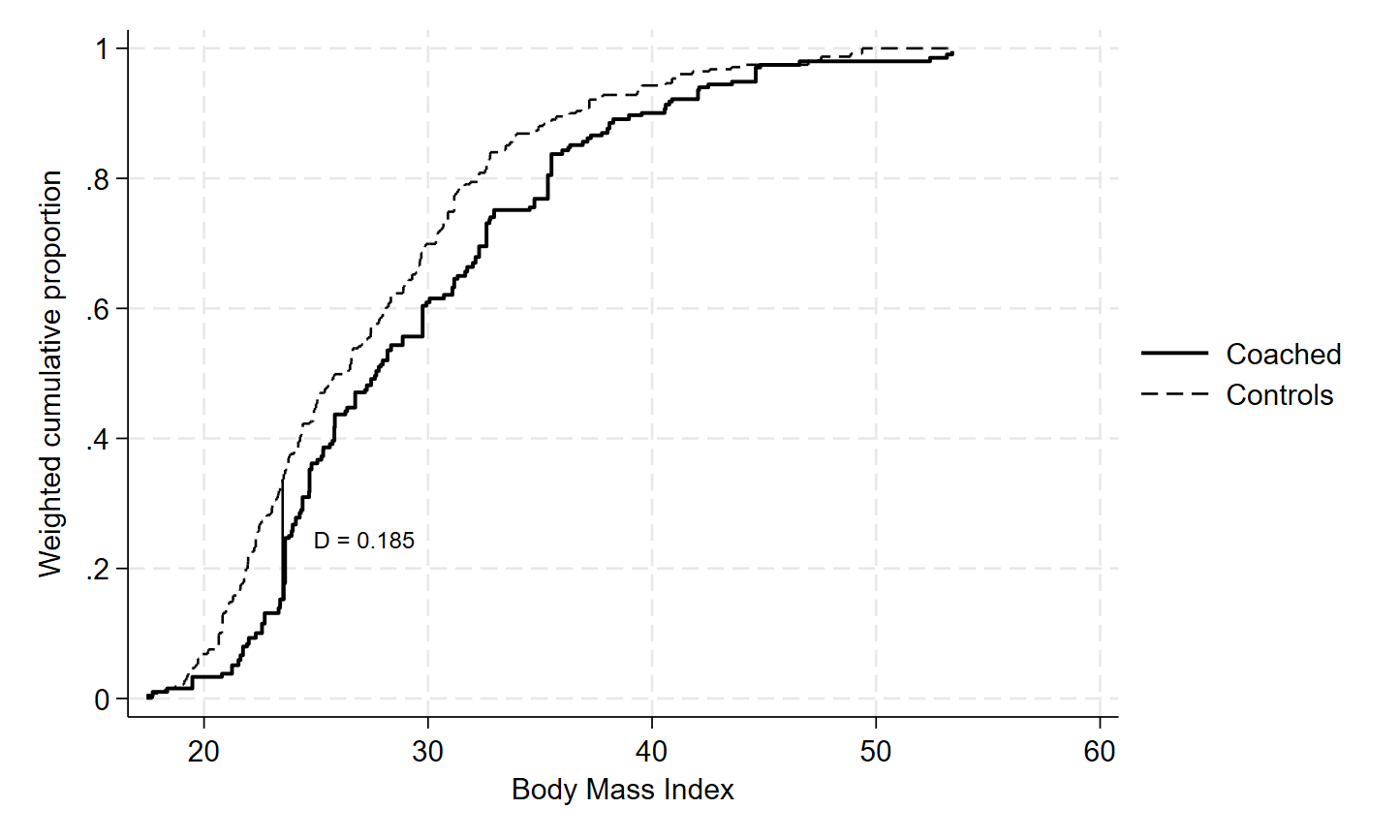
Figure 1 displays the weighted empirical CDFs of BMI for the Coached and Control groups following weighting, with the location of the Kolmogorov–Smirnov statistic marked directly on the plot. Table 6 reports the results of all three weighted tests, each based on 2000 permutation replicates.
The three tests yield materially different conclusions about the extent of residual BMI imbalance after weighting. The Anderson–Darling test detects a statistically significant discrepancy (), the Cramér–von Mises test is suggestive but falls short of conventional significance (), and the Kolmogorov–Smirnov test does not reach significance at all (). Had KS been the only test available, an investigator relying on it alone might have concluded that adequate BMI balance had been achieved, when a genuine discrepancy detectable by AD remained. This pattern is consistent with the mechanistic distinctions established in the simulation study (Sections 2.6 and 5.2). Rather than being concentrated at a single, sharply localized point in the distribution, the scenario in which KS holds a clear advantage, Figure 1 shows the Coached and Control ECDFs diverging gradually and persisting across a substantial range of BMI values before the two distributions converge in the upper tail. A discrepancy of this more diffuse character is exactly the scenario in which AD’s whole-distribution, variance-standardized summation is expected to outperform KS’s single-largest-gap statistic, consistent with what is observed here. This example illustrates directly why relying on a single distributional test could lead an investigator to different conclusions about covariate balance depending on which test happens to be chosen.
5 Discussion
5.1 Principal Findings
This study extended the Kolmogorov–Smirnov, Cramér–von Mises, and Anderson–Darling tests to accommodate case weights, using a single permutation-inference procedure applicable to any weighting scheme, and evaluated all three weighted tests across four simulation scenarios. Four principal findings emerge. First, all three weighted tests maintained rejection rates close to the nominal level across the sample sizes examined, under substantial weight variability. This close correspondence is consistent with the permutation procedure behaving as intended, since a poorly calibrated procedure would be unlikely to track the nominal rate this consistently, though a simulation study of this kind can demonstrate consistency with valid behavior rather than establish validity in general. Second, two of the three theoretically motivated comparative advantages set out in Section 2.6 were confirmed without ambiguity: KS was the most powerful test against a centrally located discrepancy, and AD was overwhelmingly the most powerful test against a tail-located discrepancy. That these unweighted comparative advantages carried over intact to the weighted setting provides further empirical support for the weighting extension, independent of the Type I error results above. Third, the theoretical expectation that CVM would be distinctly best suited to a diffuse discrepancy was only partly borne out: AD and CVM performed comparably against a uniform, whole-distribution shift, both clearly ahead of KS at every sample size, with AD acquiring a modest but statistically significant edge over CVM from a moderate sample size onward. Fourth, a follow-up check across a wider range of weight variability (Section 3.6) found this comparative ordering preserved at every level examined, with Type I error remaining close to nominal except at the most severe weight variability tested, where all three tests showed a modest, consistent upward deviation.
5.2 Mechanistic Interpretation
The centrally located and tail-located results follow directly from the mechanisms already described in Section 1: KS’s dependence on a single largest gap favors a discrepancy concentrated at one point, and AD’s variance term, largest in the tails and smallest at the center, favors a discrepancy located there. Weighting did not disturb either mechanism.
That these mechanisms carried over from the unweighted to the weighted setting is itself informative, distinct from the Type I error results above. Weighting could in principle have disrupted the qualitative behavior established for the unweighted tests, for instance if the ECDF substitution or the Kish-adjusted variance term had introduced some unanticipated distortion. Instead, the weighted tests reproduced the same comparative ordering documented for their unweighted counterparts in two of the three scenarios, matching what the theoretical construction of each statistic would predict. This agreement between theory and simulation is consistent with the weighted tests behaving as faithful generalizations of the original statistics, though it is empirical agreement under the specific conditions simulated here, not a general proof that this must hold under every possible weighting scheme and discrepancy type.
The diffuse-scenario result is more subtle, and worth interpreting carefully rather than treated as a simple confirmation of the a priori ordering. A uniform, whole-distribution location shift offers CVM’s summation a diffuse signal to accumulate across the entire support, consistent with theory. But it also offers AD’s variance-standardization term no particular region to penalize or reward: unlike the centrally located scenario, where standardization actively discounts the discrepancy, or the tail-located scenario, where it actively amplifies it, a uniform shift produces a roughly symmetric pattern of discrepancy across the distribution. This leaves AD’s tail-weighting neither a specific advantage nor a specific disadvantage relative to CVM’s uniform weighting, and the two statistics end up comparably effective.
At least three plausible explanations could produce this pattern, and the present simulation cannot fully separate them. One possibility is that AD’s variance-standardization term becomes nearly uninformative under a genuinely uniform shift: if the discrepancy is the same size everywhere, the differential weighting AD applies across the distribution has little left to differentiate, so AD behaves more like an unweighted sum, similar in spirit to CVM. A second possibility is that this is specific to the case weighting studied here and would not hold, or would hold to a different degree, under a different weight-generating mechanism or level of weight variability. A third possibility is that the result reflects something more general about how a uniform shift is a boundary case between the tail-located and centrally located scenarios, in which AD’s tail-amplification and its central discounting roughly offset one another regardless of weighting. Distinguishing among these would require additional simulation, for instance varying weight variability or the functional form of the discrepancy directly, and is a natural direction for follow-up work. The result reported here is that AD and CVM end up comparably effective against this particular type of discrepancy, both ahead of KS, rather than CVM holding a distinct advantage of its own; why this occurs mechanistically is not yet fully resolved.
5.3 Practical Advice for Investigators
The pattern of results in Sections 3.2–3.4 has direct implications for applied covariate-balance assessment after weighting. When there is reason to expect that any residual imbalance after weighting would be concentrated in a specific, narrow region of a covariate’s distribution, for example a subgroup with disproportionately similar values clustered near a particular point, KS is the most sensitive of the three tests and should be preferred. When residual imbalance is more plausibly located in the extreme values of a covariate, for example if weighting is expected to equalize central tendency but leave the most extreme treated and comparison units still poorly matched, AD is markedly more sensitive than either alternative, often by a wide margin, and should be the test of choice. This scenario is arguably the most common concern in applied propensity-score-weighted analyses, where reweighting schemes are typically constructed to balance means and low-order moments but provide no explicit guarantee about the extreme tails of a covariate’s distribution. When there is no strong prior expectation about where residual imbalance might occur, or when a broad, whole-distribution shift is the primary concern, AD and CVM perform comparably well and both outperform KS. CVM’s simpler construction, requiring no variance-standardization or effective-sample-size calculation, may make it the more convenient default in this circumstance, without a meaningful loss of power relative to AD.
Because the location of any true residual imbalance is rarely known in advance in applied work, and because AD matched or exceeded CVM’s performance in every scenario examined here while also being overwhelmingly the best test for tail-located discrepancies, AD appears to be a reasonable general-purpose default for routine covariate-balance diagnostics that can only accommodate a single test. Investigators with a specific reason to suspect a centrally concentrated imbalance rather than a tail-located or diffuse one may still find KS more powerful in that particular circumstance. Given the complementary sensitivities documented here, reporting more than one test, for example both AD and KS, is a reasonable and inexpensive way to guard against the blind spots of any single statistic. In any case, investigators should report the process they used to inform their ultimate choice of test (Linden and Roberts,, 2005; Linden et al.,, 2003).
One additional practical caveat concerns covariates with a substantial point mass at a single value, such as an earnings variable with many observations at exactly zero. AD’s tie multiplier (Section 2.4) is retained as the raw, unweighted count of observations sharing a value, and a large tie block can therefore contribute disproportionately to the observed AD statistic regardless of the weights involved. Investigators working with semi-continuous covariates of this kind should be aware that a significant AD result may be driven substantially by the size of a tie block at a single point rather than by a genuinely broader distributional discrepancy, and may wish to additionally inspect the covariate’s distribution directly rather than relying on the test statistic alone.
5.4 Limitations
Several limitations should be noted. First, the data-generating process used a normal base distribution throughout, with discrepancies introduced as controlled shifts at specific quantiles or across the whole distribution. This was a deliberate choice. The aim was to isolate how each test responds to a discrepancy of a known location and character. A differently shaped base distribution, for instance skewed, bimodal, or heavy-tailed, would add a second source of variation alongside the discrepancy itself. Any resulting difference in test performance would then be harder to attribute to the discrepancy’s location rather than to the base distribution’s shape. Whether the comparative ordering documented here extends to non-normal base distributions was not assessed and is a natural direction for follow-up work.
Second, each discrepancy type was examined at a single, fixed effect size across four sample sizes, rather than varying effect size at a fixed sample size; the resulting power curves should be interpreted as power against one specific magnitude of discrepancy of each type, not as a general power surface across discrepancy magnitude and sample size jointly.
Finally, computational cost was not evaluated as a formal outcome, on the grounds that these tests are intended for routine, one-time covariate-balance assessment in applied analyses rather than repeated use inside larger simulation pipelines, where runtime considerations would carry more weight.
5.5 Conclusion
This paper makes two contributions. It extends the Kolmogorov–Smirnov, Cramér–von Mises, and Anderson–Darling tests to weighted data for the first time, and it does so through a single label-permutation inference procedure that requires no assumption about how a given weight was generated. This generality, applicable to any weighting scheme, is what distinguishes the approach from a method built around one specific weighting mechanism. Both contributions were supported by two independent empirical patterns in a four-scenario simulation study: rejection rates that clustered near the nominal level under a true null, and the preservation, under weighting, of comparative advantages already well established for the unweighted tests. All three tests controlled Type I error correctly under substantial weight variability. Each test’s known unweighted comparative advantage was preserved under weighting for centrally located and tail-located discrepancies, with AD and CVM performing comparably, rather than CVM alone dominating, against a diffuse discrepancy. These findings support AD as a reasonable general-purpose default for routine covariate-balance assessment, while noting that KS retains a distinct and substantial advantage when a centrally concentrated discrepancy is specifically suspected. A natural direction for future research is to extend the same weighting and permutation-inference framework to other empirical-distribution-function tests, such as the Kuiper test (Kuiper,, 1960), which sums the largest positive and negative deviations rather than the single largest absolute one, and the Wasserstein (earth-mover’s) distance (Ramdas et al.,, 2017), which measures discrepancy in the scale of the covariate itself rather than in probability.
References
- Anderson and Darling, (1952) Anderson, T. W. and Darling, D. A. (1952). Asymptotic theory of certain “goodness of fit” criteria based on stochastic processes. Annals of Mathematical Statistics, 23(2):193–212.
- Austin, (2009) Austin, P. C. (2009). Balance diagnostics for comparing the distribution of baseline covariates between treatment groups in propensity-score matched samples. Statistics in Medicine, 28(25):3083–3107.
- Austin, (2015) Austin, P. C. (2015). Moving towards best practice when using inverse probability of treatment weighting (iptw) using the propensity score to estimate causal treatment effects in observational studies. Statistics in Medicine, 34(28):3661–3679.
- Cramér, (1928) Cramér, H. (1928). On the composition of elementary errors. Scandinavian Actuarial Journal, 1928(1):13–74.
- D’Agostino and Stephens, (1986) D’Agostino, R. B. and Stephens, M. A., editors (1986). Goodness-of-Fit Techniques. Marcel Dekker, New York.
- Hainmueller, (2012) Hainmueller, J. (2012). Entropy balancing: A multivariate reweighting method to produce balanced samples in observational studies. Political Analysis, 20:25–46.
- Kish, (1965) Kish, L. (1965). Survey Sampling. John Wiley & Sons, New York.
- Kolmogorov, (1933) Kolmogorov, A. (1933). Sulla determinazione empirica di una legge di distribuzione. Giornale dell’Istituto Italiano degli Attuari, 4:83–91.
- Kuiper, (1960) Kuiper, N. H. (1960). Tests concerning random points on a circle. Proceedings of the Koninklijke Nederlandse Akademie van Wetenschappen, Series A, 63:38–47.
- Linden, (2014) Linden, A. (2014). Combining propensity score-based stratification and weighting to improve causal inference in the evaluation of health care interventions. Journal of Evaluation in Clinical Practice, 20:1065–1071.
- (11) Linden, A. (2025a). ADTEST: Stata module to perform a two-sample anderson-darling equality-of-distributions test. Statistical Software Components S459559, Boston College Department of Economics.
- (12) Linden, A. (2025b). CVMTEST: Stata module to perform a two-sample cramer-von mises equality-of-distributions test. Statistical Software Components S459558, Boston College Department of Economics.
- Linden, (2026) Linden, A. (2026). KSTEST: Stata module to perform a weighted two-sample kolmogorov-smirnov equality-of-distributions test. Statistical Software Components s459801, Boston College Department of Economics.
- Linden et al., (2003) Linden, A., Adams, J., and Roberts, N. (2003). Evaluation methods in disease management: determining program effectiveness. Position Paper for the Disease Management Association of America (DMAA).
- Linden et al., (2010) Linden, A., Butterworth, S. W., and Prochaska, J. O. (2010). Motivational interviewing-based health coaching as a chronic care intervention. Journal of Evaluation in Clinical Practice, 16(1):166–174.
- Linden and Roberts, (2005) Linden, A. and Roberts, N. (2005). A user’s guide to the disease management literature: recommendations for reporting and assessing program outcomes. American Journal of Managed Care, 11:113–120.
- Linden and Samuels, (2013) Linden, A. and Samuels, S. (2013). Using balance statistics to determine the optimal number of controls in matching studies. Journal of Evaluation in Clinical Practice, 19(5):968–975.
- Linden and Yarnold, (2016) Linden, A. and Yarnold, P. (2016). Using machine learning to assess covariate balance in matching studies. Journal of Evaluation in Clinical Practice, 22:848–854.
- Linden and Yarnold, (2017) Linden, A. and Yarnold, P. (2017). Using classification tree analysis to generate propensity score weights. Journal of Evaluation in Clinical Practice, 23:703–712.
- Linden and Yarnold, (2018) Linden, A. and Yarnold, P. (2018). Estimating causal effects for survival (time-to-event) outcomes by combining classification tree analysis and propensity score weighting. Journal of Evaluation in Clinical Practice, 24:380–387.
- Newson and Falcaro, (2023) Newson, R. and Falcaro, M. (2023). Robit regression in stata. The Stata Journal, 3:658–682.
- Pettitt, (1976) Pettitt, A. N. (1976). A two-sample Anderson–Darling rank statistic. Biometrika, 63(1):161–168.
- Ramdas et al., (2017) Ramdas, A., Garcia, N., and Cuturi, M. (2017). On Wasserstein two-sample testing and related families of nonparametric tests. Entropy, 19:47.
- Robins et al., (2000) Robins, J., Hernan, M., and Brumback, B. (2000). Marginal structural models and causal inference in epidemiology. Epidemiology, 11:550–560.
- Rubin, (1973) Rubin, D. B. (1973). Matching to remove bias in observational studies. Biometrics, 29:159–184.
- Rubin, (2008) Rubin, D. B. (2008). For objective causal inference, design trumps analysis. Annals of Applied Statistics, 2:808–840.
- Scholz and Stephens, (1987) Scholz, F. W. and Stephens, M. A. (1987). K-sample Anderson–Darling tests. Journal of the American Statistical Association, 82(399):918–924.
- Smirnov, (1948) Smirnov, N. (1948). Table for estimating the goodness of fit of empirical distributions. Annals of Mathematical Statistics, 19(2):279–281.
- Stephens, (1974) Stephens, M. A. (1974). EDF statistics for goodness of fit and some comparisons. Journal of the American Statistical Association, 69(347):730–737.
- Stuart, (2010) Stuart, E. A. (2010). Matching methods for causal inference: a review and a look forward. Statistical Science, 25(1):1–21.
- von Mises, (1931) von Mises, R. (1931). Wahrscheinlichkeitsrechnung und ihre Anwendung in der Statistik und theoretischen Physik. Deuticke, Leipzig.
| Purpose | Shift function |
|---|---|
| Type I error | |
| Power: centrally located | Localized: at , at , , |
| Power: tail-located | Localized: at , at , , |
| Power: diffuse | (uniform shift) |
Note: all four scenarios were run at total sample size , with , throughout. Case weights follow a lognormal distribution targeting a Kish effective-sample-size ratio of (see text), assigned independently of the DGP. Total scenario-by-sample-size combinations: ; 2000 replications per combination; permutation replicates per test per replicate.
| KS | AD | CVM | |
|---|---|---|---|
| 1000 | .055 (.045, .065) | .048 (.039, .057) | .050 (.040, .060) |
| 2000 | .044 (.035, .053) | .044 (.035, .053) | .046 (.037, .055) |
| 3000 | .043 (.034, .052) | .043 (.034, .052) | .042 (.033, .051) |
| 4000 | .055 (.045, .065) | .057 (.047, .067) | .057 (.047, .067) |
Note: 2000 replications per cell; values in parentheses are 95% confidence intervals ().
| Scenario | KS | AD | CVM | |
|---|---|---|---|---|
| Centrally located | 1000 | .449 (.427, .471) | .193 (.176, .210) | .146 (.131, .161) |
| 2000 | .840 (.824, .856) | .448 (.426, .470) | .323 (.303, .343) | |
| 3000 | .973 (.966, .980) | .703 (.683, .723) | .579 (.557, .601) | |
| 4000 | .996 (.993, .999) | .912 (.900, .924) | .828 (.811, .845) | |
| Tail-located | 1000 | .045 (.036, .054) | .114 (.100, .128) | .051 (.041, .061) |
| 2000 | .049 (.040, .058) | .297 (.277, .317) | .060 (.050, .070) | |
| 3000 | .081 (.069, .093) | .655 (.634, .676) | .072 (.061, .083) | |
| 4000 | .137 (.122, .152) | .914 (.902, .926) | .072 (.061, .083) | |
| Diffuse | 1000 | .183 (.166, .200) | .215 (.197, .233) | .205 (.187, .223) |
| 2000 | .309 (.289, .329) | .376 (.355, .397) | .358 (.337, .379) | |
| 3000 | .441 (.419, .463) | .512 (.490, .534) | .495 (.473, .517) | |
| 4000 | .536 (.514, .558) | .648 (.627, .669) | .618 (.597, .639) |
Note: 2000 replications per cell; rejection rate at using each test’s permutation p-value ( replicates). Values in parentheses are 95% confidence intervals (). See Table 4 for paired-difference significance tests.
| AD KS | CVM KS | AD CVM | |||||
|---|---|---|---|---|---|---|---|
| Scenario | |||||||
| Type I error | 1000 | .007 | .262 | .005 | .369 | .002 | .593 |
| 2000 | .000 | 1.000 | .002 | .670 | .002 | .617 | |
| 3000 | .000 | 1.000 | .001 | .847 | .001 | .782 | |
| 4000 | .002 | .746 | .002 | .715 | .000 | 1.000 | |
| Centrally located | 1000 | .256 | .001 | .303 | .001 | .047 | .001 |
| 2000 | .392 | .001 | .517 | .001 | .125 | .001 | |
| 3000 | .270 | .001 | .394 | .001 | .124 | .001 | |
| 4000 | .084 | .001 | .168 | .001 | .084 | .001 | |
| Tail-located | 1000 | .069 | .001 | .006 | .273 | .063 | .001 |
| 2000 | .248 | .001 | .011 | .093 | .237 | .001 | |
| 3000 | .574 | .001 | .009 | .225 | .583 | .001 | |
| 4000 | .777 | .001 | .065 | .001 | .842 | .001 | |
| Diffuse | 1000 | .032 | .001 | .022 | .003 | .010 | .140 |
| 2000 | .067 | .001 | .049 | .001 | .018 | .016 | |
| 3000 | .071 | .001 | .054 | .001 | .017 | .029 | |
| 4000 | .112 | .001 | .082 | .001 | .030 | .001 | |
Note: is the mean per-replicate difference in rejection outcome (e.g., ADKS: positive values indicate AD rejected more often than KS on the same simulated datasets); -values are from a paired -test using the standard deviation of the per-replicate difference, which correctly accounts for the correlation between tests run on identical data. shown where the exact value rounds to at three decimal places.
| Condition | KS | AD | CVM | |
|---|---|---|---|---|
| Type I error (null) | 0.2 | .064 | .067 | .064 |
| 0.4 | .048 | .064 | .056 | |
| 0.6 | .044 | .044 | .046 | |
| 0.8 | .046 | .041 | .041 | |
| 0.9 | .056 | .054 | .061 | |
| Power: centrally located | 0.2 | .317 | .138 | .108 |
| 0.4 | .576 | .251 | .193 | |
| 0.6 | .840 | .448 | .323 | |
| 0.8 | .953 | .623 | .497 | |
| 0.9 | .978 | .694 | .571 | |
| Power: tail-located | 0.2 | .052 | .101 | .059 |
| 0.4 | .053 | .182 | .068 | |
| 0.6 | .049 | .297 | .060 | |
| 0.8 | .064 | .538 | .066 | |
| 0.9 | .065 | .653 | .063 | |
| Power: diffuse | 0.2 | .144 | .164 | .161 |
| 0.4 | .206 | .252 | .239 | |
| 0.6 | .309 | .376 | .358 | |
| 0.8 | .379 | .433 | .438 | |
| 0.9 | .439 | .526 | .513 |
Note: 2000 replications per cell; sample size fixed at (, ) throughout, extending the single value of used in Table 2 and Table 3 to a range from milder (, ) to more severe (, ) weight variability. All values are rejection rates at : for the “Type I error” rows, this is the empirical size under the null (no true discrepancy); for the three “Power” rows, this is empirical power against the discrepancy named. The row in each panel reproduces the corresponding cell from Table 2 (Type I error) or Table 3 (power).
| Test | Statistic | -value |
|---|---|---|
| Kolmogorov–Smirnov | .123 | |
| Anderson–Darling | .018 | |
| Cramér–von Mises | .079 |
Note: all three tests based on 2000 permutation replicates, seed 12345. Raw statistic magnitudes are not comparable across tests; significance is determined entirely by each test’s own permutation null distribution, not by the absolute size of its statistic.