跳到论文正文
W Papers独立论文阅读器 arXiv:2607.20845 论文正文 计算阅读时间 · 0%
引用这篇论文根据当前论文元数据生成,正式投稿前建议核对。


License: arXiv.org perpetual non-exclusive license
arXiv:2607.20845v1 [math.OC] 23 Jul 2026

Mean field and N-agent games for optimal relative consumption-investment with jump risk and common noise

Yiming Jiang, Fuxing Li, Yawei Wei, Zimeng Zheng
Abstract

This paper studies an optimal consumption–investment problem for competitive agents in an NN-player game and its associated mean field game. Each agent invests in an individual risky asset subject to idiosyncratic noise, common noise and downward jump risk, and the interaction among agents is induced by relative performance concerns in both consumption and terminal wealth. In the mean field limit, we characterize a deterministic mean field equilibrium in analytical form by using the stochastic maximum principle. Numerical experiments are presented to illustrate the resulting equilibrium and its financial implications. Finally, based on the obtained mean field equilibrium, we construct an approximate Nash equilibrium for the NN-player game. This model is motivated by [34] and [27].

1 Introduction and main results

We consider a large financial market populated by NN agents sharing a common finite time horizon [0,T][0,T], where T>0T>0. Each agent ii may invest in a common riskless bond with zero interest rate or in an individual stock ii. For i=1,…,Ni=1,\ldots,N, the price process of stock ii is given by the following stochastic differential equation (SDE):

d​StiSt−i=bi​d​t+σi​d​Wti+σi0​d​Wt0−d​Mti,t∈[0,T]\frac{dS_{t}^{i}}{S_{t-}^{i}}=b_{i}dt+\sigma_{i}dW_{t}^{i}+\sigma_{i}^{0}dW_{t}^{0}-dM_{t}^{i},\qquad t\in[0,T] (1)

with constant parameters bi>0b_{i}>0 and σi,σi0>0\sigma_{i},\sigma_{i}^{0}>0. Here, W0=(Wt0)t∈[0,T]W^{0}=(W_{t}^{0})_{t\in[0,T]} appears in the price dynamics of all agents and represents the common noise in the financial market, while Wi=(Wti)t∈[0,T]W^{i}=(W_{t}^{i})_{t\in[0,T]} denotes the idiosyncratic noise associated with agent ii. The Brownian motions W0,W1,…,WNW^{0},W^{1},\ldots,W^{N} are independent on a filtered probability space (Ω,ℱ,𝔽,ℙ)(\Omega,\mathcal{F},\mathbb{F},\mathbb{P}), where 𝔽=(ℱt)t∈[0,T]\mathbb{F}=(\mathcal{F}_{t})_{t\in[0,T]} satisfies the usual conditions. Moreover, we set the filtration 𝔽0=(ℱt0)t∈[0,T]=(σ​(Ws0;s≤t))t∈[0,T]\mathbb{F}^{0}=\left(\mathcal{F}^{0}_{t}\right)_{t\in[0,T]}=\left(\sigma\left(W_{s}^{0};s\leq t\right)\right)_{t\in[0,T]}. In the above equation, Mi=(Mti)t∈[0,T]M^{i}=(M_{t}^{i})_{t\in[0,T]} denotes the compensated process of Ni=(Nti)t∈[0,T]N^{i}=(N_{t}^{i})_{t\in[0,T]}, where NiN^{i} is a Poisson process with intensity λi\lambda_{i}. The presence of MiM^{i} allows the stock price to be subject to downward jump risk, a classical modeling feature already considered by Merton [35]. In particular, the Poisson processes N1,…,NNN^{1},\ldots,N^{N} are mutually independent and independent of the Brownian motions W0,W1,…,WNW^{0},W^{1},\ldots,W^{N}. We define the global market filtration 𝔾=(𝒢t)t∈[0,T]=(ℱt∨σ​((Ns1,…,NsN)⊤; 0≤s≤t))t∈[0,T]\mathbb{G}=(\mathcal{G}_{t})_{t\in[0,T]}=(\mathcal{F}_{t}\vee\sigma((N^{1}_{s},\ldots,N^{N}_{s})^{\top};\,0\leq s\leq t))_{t\in[0,T]} as the right-continuous augmentation by ℙ\mathbb{P}-null sets. Then, for each i=1,…,Ni=1,\ldots,N, the compensated process Mti=Nti−λi​tM_{t}^{i}=N_{t}^{i}-\lambda_{i}t is a (ℙ,𝔾)(\mathbb{P},\mathbb{G})-martingale on [0,T][0,T]. In addition, the Brownian motions W0,W1,…,WNW^{0},W^{1},\ldots,W^{N} remain Brownian motions with respect to 𝔾\mathbb{G}. A similar filtration setting can be found in Bo et al. [7].

For i=1,…,Ni=1,\ldots,N, let πi=(πti)t∈[0,T]\pi^{i}=(\pi_{t}^{i})_{t\in[0,T]} denote the proportion of wealth that agent ii invests in stock ii, and let ci=(cti)t∈[0,T]c^{i}=(c_{t}^{i})_{t\in[0,T]} denote the instantaneous consumption rate per unit wealth of agent ii. Then the corresponding self-financing wealth processes Xi=(Xti)t∈[0,T]X^{i}=(X_{t}^{i})_{t\in[0,T]} satisfy the following SDE:

{d​Xti=(πti​bi−cti)​Xti​d​t+πti​Xti​σi​d​Wti+πti​Xti​σi0​d​Wt0−πti​Xt−i​d​Mti,X0i=x0i,\left\{\begin{aligned} &dX_{t}^{i}=\left(\pi_{t}^{i}b_{i}-c_{t}^{i}\right)X_{t}^{i}dt+\pi_{t}^{i}X_{t}^{i}\sigma_{i}dW_{t}^{i}+\pi_{t}^{i}X_{t}^{i}\sigma_{i}^{0}dW_{t}^{0}-\pi_{t}^{i}X_{t-}^{i}dM_{t}^{i},\\ &X_{0}^{i}=x_{0}^{i},\end{aligned}\right. (2)

where x0i>0x_{0}^{i}>0 denotes the initial wealth of agent ii. We now introduce the admissible control set for each agent.

Definition 1.1 (Admissible control set for agent ii).

For each agent i=1,…,Ni=1,\ldots,N, the admissible control set 𝒜i\mathcal{A}_{i} consists of all pairs of processes (πi,ci)=(πti,cti)t∈[0,T](\pi^{i},c^{i})=(\pi_{t}^{i},c_{t}^{i})_{t\in[0,T]} such that πi\pi^{i} is 𝔾\mathbb{G}-predictable, cic^{i} is 𝔾\mathbb{G}-progressively measurable,

(πti,cti)∈[D0,1−ϵ0]×(0,∞)for all ​t∈[0,T],ℙ​-a.s.,(\pi_{t}^{i},c_{t}^{i})\in[D_{0},1-\epsilon_{0}]\times(0,\infty)\quad\text{for all }t\in[0,T],\quad\mathbb{P}\text{-a.s.},

and

∫0Tcti​𝑑t<∞,ℙ​-a.s.\int_{0}^{T}c_{t}^{i}\,dt<\infty,\qquad\mathbb{P}\text{-a.s.}

Here D0∈ℝD_{0}\in\mathbb{R} is a constant and ϵ0∈(0,1)\epsilon_{0}\in(0,1) is a sufficiently small constant.

Remark 1.2.

The admissibility conditions are imposed to ensure that the wealth equation (2) is well-posed and that the corresponding wealth process remains strictly positive. In particular, the lower bound D0D_{0} rules out unbounded short positions, while the constraint πti≤1−ϵ0\pi_{t}^{i}\leq 1-\epsilon_{0} prevents bankruptcy after a downward jump, since Xti=Xt−i​(1−πti)>0X_{t}^{i}=X_{t-}^{i}(1-\pi_{t}^{i})>0.

The aim of agent ii is to maximize the following objective functional over all admissible strategies (πi,ci)∈𝒜i(\pi^{i},c^{i})\in\mathcal{A}_{i}:

Ji​((πi,ci)i=1N)=𝔼​[∫0TU​(cti​Xti​(ct​Xt¯)−θi;γi)​𝑑t+εi​U​(XTi​XT¯−θi;γi)],J_{i}((\pi^{i},c^{i})_{i=1}^{N})=\mathbb{E}\left[\int_{0}^{T}U(c_{t}^{i}X_{t}^{i}(\overline{c_{t}X_{t}})^{-\theta_{i}};\gamma_{i})dt+\varepsilon_{i}U(X_{T}^{i}\overline{X_{T}}^{-\theta_{i}};\gamma_{i})\right], (3)

where U​(x;γ)=1γ​xγU(x;\gamma)=\frac{1}{\gamma}x^{\gamma} is a constant relative risk aversion (CRRA) utility function. Moreover, ct​Xt¯:=(ct1​Xt1​⋯​ctN​XtN)1/N\overline{c_{t}X_{t}}:=\left(c_{t}^{1}X_{t}^{1}\cdots c_{t}^{N}X_{t}^{N}\right)^{1/N} and XT¯:=(XT1​⋯​XTN)1/N\overline{X_{T}}:=\left(X_{T}^{1}\cdots X_{T}^{N}\right)^{1/N} denote the population geometric averages of consumption and terminal wealth, respectively. The parameters γi∈(0,1)\gamma_{i}\in(0,1) and θi∈[0,1]\theta_{i}\in[0,1] characterize the risk preference and the competition weight of agent ii, while εi>0\varepsilon_{i}>0 measures the relative importance assigned to terminal wealth.

In the presence of jump risk in the wealth dynamics (2), the explicit characterization of Nash equilibrium strategies for the NN-agent game is generally intractable. Nevertheless, we can construct an approximate Nash equilibrium for the NN-agent system. The definition is given as follows.

Definition 1.3 (Approximate Nash equilibrium).

An admissible strategy profile

(𝝅∗,𝒄∗)=((π∗,1,c∗,1),…,(π∗,N,c∗,N))∈𝒜1×⋯×𝒜N(\bm{\pi}^{*},\bm{c}^{*})=\left((\pi^{*,1},c^{*,1}),\ldots,(\pi^{*,N},c^{*,N})\right)\in\mathcal{A}_{1}\times\cdots\times\mathcal{A}_{N}

is called a uNu_{N}-Nash equilibrium if there exists a sequence uN→0u_{N}\to 0 as N→∞N\to\infty such that, for every i=1,…,Ni=1,\ldots,N,

sup(πi,ci)∈𝒜iJi​((πi,ci),(𝝅∗,𝒄∗)−i)⩽Ji​((π∗,i,c∗,i),(𝝅∗,𝒄∗)−i)+uN.\sup_{(\pi^{i},c^{i})\in\mathcal{A}_{i}}J_{i}\left((\pi^{i},c^{i}),(\bm{\pi}^{*},\bm{c}^{*})^{-i}\right)\leqslant J_{i}\left((\pi^{*,i},c^{*,i}),(\bm{\pi}^{*},\bm{c}^{*})^{-i}\right)+u_{N}.

Here,

(𝝅∗,𝒄∗)−i:=((π∗,1,c∗,1),…,(π∗,i−1,c∗,i−1),(π∗,i+1,c∗,i+1),…,(π∗,N,c∗,N)).(\bm{\pi}^{*},\bm{c}^{*})^{-i}:=\left((\pi^{*,1},c^{*,1}),\ldots,(\pi^{*,i-1},c^{*,i-1}),(\pi^{*,i+1},c^{*,i+1}),\ldots,(\pi^{*,N},c^{*,N})\right).

We first consider the limiting case as N→∞N\to\infty. Before introducing the representative agent model, we impose the following assumption throughout this paper.

Assumption 1.4.

For each i=1,…,Ni=1,\ldots,N, define the type vector by

ξi:=(x0i,λi,bi,σi,σi0,εi,γi,θi)∈𝒪:=𝒦×[γ¯,γ¯]×[0,1],\xi^{i}:=\left(x_{0}^{i},\lambda_{i},b_{i},\sigma_{i},\sigma_{i}^{0},\varepsilon_{i},\gamma_{i},\theta_{i}\right)\in\mathcal{O}:=\mathcal{K}\times[\underline{\gamma},\overline{\gamma}]\times[0,1],

where 𝒦\mathcal{K} is a compact subset of (0,∞)6(0,\infty)^{6}, and 0<γ¯<γ¯<10<\underline{\gamma}<\overline{\gamma}<1. Let ℬ​(𝒪)\mathcal{B}(\mathcal{O}) denote the Borel σ\sigma-algebra on 𝒪\mathcal{O}. Assume that there exists a constant vector

ξ:=(x0,λ,b,σ,σ0,ε,γ,θ)∈𝒪\xi:=\left(x_{0},\lambda,b,\sigma,\sigma^{0},\varepsilon,\gamma,\theta\right)\in\mathcal{O}

such that

ν0N:=1N​∑i=1Nδξi⇒ν0:=δξas ​N→∞,\nu_{0}^{N}:=\frac{1}{N}\sum_{i=1}^{N}\delta_{\xi^{i}}\Rightarrow\nu_{0}:=\delta_{\xi}\quad\text{as }N\to\infty,

where ν0N\nu_{0}^{N} denotes the empirical probability measure on ℬ​(𝒪)\mathcal{B}(\mathcal{O}), and “⇒\Rightarrow” denotes weak convergence, that is, for every bounded continuous function ff,

∫𝒪f​𝑑ν0N→∫𝒪f​𝑑ν0as ​N→∞.\int_{\mathcal{O}}f\,d\nu_{0}^{N}\to\int_{\mathcal{O}}f\,d\nu_{0}\quad\text{as }N\to\infty.

As N→∞N\to\infty, Assumption 1.4 leads to the following SDE of the wealth process for the representative agent,

{d​Xt=(πt​b−ct)​Xt​d​t+πt​Xt​σ​d​Wt+πt​Xt​σ0​d​Wt0−πt​Xt−​d​MtX0=x0\left\{\begin{aligned} &dX_{t}=\left(\pi_{t}b-c_{t}\right)X_{t}dt+\pi_{t}X_{t}\sigma dW_{t}+\pi_{t}X_{t}\sigma^{0}dW_{t}^{0}-\pi_{t}X_{t-}dM_{t}\\ &X_{0}=x_{0}\end{aligned}\right. (4)

where W=(Wt)t∈[0,T]W=(W_{t})_{t\in[0,T]} is a scalar Brownian motion independent of the Brownian motions (W0,W1,…,WN)(W^{0},W^{1},\ldots,W^{N}), and M=(Mt)t∈[0,T]M=(M_{t})_{t\in[0,T]} is given by Mt=Nt−λ​tM_{t}=N_{t}-\lambda t, with N=(Nt)t∈[0,T]N=(N_{t})_{t\in[0,T]} being a Poisson process with intensity λ\lambda. Let 𝔾M=(𝒢tM)t∈[0,T]\mathbb{G}^{M}=(\mathcal{G}^{M}_{t})_{t\in[0,T]} be the filtration generated by WW, W0W^{0}, and NN. Similar to Definition 1.1, the admissible control set for the representative agent 𝒜M\mathcal{A}_{M} is defined analogously, replacing the filtration 𝔾\mathbb{G} with 𝔾M\mathbb{G}^{M}.

Since the influence of any single agent’s strategy pair on the population is negligible, we replace the geometric averages of the wealth and consumption with given processes (m,Γ)(m,\Gamma), and the objective functional of the representative agent associated with an admissible control (π,c)∈𝒜M(\pi,c)\in\mathcal{A}_{M} is defined by

J​(π,c)=𝔼​[∫0TU​(ct​Xt​(Γt​mt)−θ;γ)​𝑑t+ε​U​(XT​mT−θ;γ)].J(\pi,c)=\mathbb{E}\left[\int_{0}^{T}U(c_{t}X_{t}(\Gamma_{t}m_{t})^{-\theta};\gamma)dt+\varepsilon U(X_{T}m_{T}^{-\theta};\gamma)\right]. (5)

In the mean field limit, agents are expected to exhibit symmetric and identical behavior. Consequently, the geometric mean of wealth and consumption (m,Γ)(m,\Gamma) must coincide with the conditional geometric averages generated by the optimal response of the representative agent. This idea leads to the consistency condition in mean field games, which forms the basis for the definition of a mean field equilibrium.

Definition 1.5 (Mean field equilibrium (MFE)).

For given 𝔽0\mathbb{F}^{0}-adapted processes mm and Γ\Gamma, let π∗,m,Γ=(πt∗,m,Γ)t∈[0,T]\pi^{*,m,\Gamma}=(\pi_{t}^{*,m,\Gamma})_{t\in[0,T]} and c∗,m,Γ=(ct∗,m,Γ)t∈[0,T]c^{*,m,\Gamma}=(c_{t}^{*,m,\Gamma})_{t\in[0,T]} be the optimal control for the control problem (4)–(5). Then, the pair (π∗,m∗,Γ∗,c∗,m∗,Γ∗)\bigl(\pi^{*,m^{*},\Gamma^{*}},c^{*,m^{*},\Gamma^{*}}\bigr) is called a mean field equilibrium if there exist (m∗,Γ∗)(m^{*},\Gamma^{*}) such that

  1. (i)

    (π∗,m∗,Γ∗,c∗,m∗,Γ∗)\bigl(\pi^{*,m^{*},\Gamma^{*}},c^{*,m^{*},\Gamma^{*}}\bigr) is an optimal control pair for the control problem (4)–(5) associated with (m∗,Γ∗)(m^{*},\Gamma^{*});

  2. (ii)

    (m∗,Γ∗)(m^{*},\Gamma^{*}) satisfies the consistency condition

    {mt∗=exp⁡{𝔼​[ln⁡(Xt∗,m∗,Γ∗)∣ℱt0]},t∈[0,T],Γt∗=exp⁡{𝔼​[ln⁡(ct∗,m∗,Γ∗)∣ℱt0]},t∈[0,T],\left\{\begin{aligned} m_{t}^{*}&=\exp\left\{\mathbb{E}\left[\ln\left(X_{t}^{*,m^{*},\Gamma^{*}}\right)\mid\mathcal{F}_{t}^{0}\right]\right\},\quad t\in[0,T],\\ \Gamma_{t}^{*}&=\exp\left\{\mathbb{E}\left[\ln\left(c_{t}^{*,m^{*},\Gamma^{*}}\right)\mid\mathcal{F}_{t}^{0}\right]\right\},\quad t\in[0,T],\end{aligned}\right. (6)

    where X∗,m∗,Γ∗=(Xt∗,m∗,Γ∗)t∈[0,T]X^{*,m^{*},\Gamma^{*}}=(X_{t}^{*,m^{*},\Gamma^{*}})_{t\in[0,T]} is the wealth process associated with π∗,m∗,Γ∗\pi^{*,m^{*},\Gamma^{*}} and c∗,m∗,Γ∗c^{*,m^{*},\Gamma^{*}}.

If, in addition, both π∗,m∗,Γ∗\pi^{*,m^{*},\Gamma^{*}} and c∗,m∗,Γ∗c^{*,m^{*},\Gamma^{*}} are deterministic, then (π∗,m∗,Γ∗,c∗,m∗,Γ∗)\bigl(\pi^{*,m^{*},\Gamma^{*}},c^{*,m^{*},\Gamma^{*}}\bigr) is called a deterministic mean field equilibrium.

The continuous-time consumption and investment problem has been a central topic in mathematical finance since the seminal contribution of Merton [33, 34, 35]. In these papers, Merton established the foundational framework for consumption and portfolio management, formulated the classical expected utility maximization problem, and incorporated jump-diffusion dynamics into asset price modeling. This line of research has since been extensively developed in multiple directions; see, for example, [17, 19, 18]. In the classical Merton model, agents focus only on their own performance, while in real markets, investment decisions are often influenced by peers. The economic motivation for relative performance concerns dates back to Veblen’s theory of conspicuous consumption [38] and Duesenberry’s relative income hypothesis [21], and was later formalized by Abel [1] through utility specifications involving relative consumption. Such criteria have been widely used to model competition among investors, fund managers, and financial institutions, see [9, 16, 26]. Since relative performance concerns couple agents’ decisions, the resulting problems are naturally formulated as stochastic differential games. Several related contributions have considered the finite-player setting [10, 3, 22].

As the number of players increases, the coupling among agents through relative performance terms may cause classical methods to suffer from the curse of dimensionality, making the direct characterization of Nash equilibria generally intractable. To overcome this difficulty, Lasry and Lions [29] introduced mean field game (MFG) theory, while a closely related approach was independently developed by Huang et al. [25]. The key idea of MFG theory is that, when the number of players is sufficiently large, the coupling interactions among individuals can be replaced by the interaction between a representative agent and the population distribution, which substantially reduces the complexity of the original game and provides a powerful framework for analyzing large-population systems. So far, the MFG framework has since been applied to a wide range of areas; we refer the reader to [24, 14, 15, 31] and the references therein. In large-population financial models with relative performance concerns, the MFG approach has proved particularly useful. Lacker and Zariphopoulou [28] studied optimal investment games under relative performance criteria and constructed explicit equilibrium strategies for both finite-agent games and their mean field limits under CARA and CRRA utilities. Lacker and Soret [27] extended this framework to a consumption-investment model and derived closed-form solutions for both the finite-agent game and the corresponding MFG under CRRA utilities. Bo et al. [8] studied optimal investment and consumption problems for large populations under external habit formation. They derived mean field equilibria under both linear and multiplicative external habit formation and showed that approximate Nash equilibria for the finite-agent games can be constructed from the corresponding mean field equilibria. Liang and Zhang [32] further investigated an optimal investment-consumption problem with heterogeneous agents, where the average habit formation and average wealth of peers serve as performance benchmarks. They obtained closed-form mean field equilibria and constructed approximate Nash equilibria for the corresponding finite-agent game.

The above studies are mainly developed within the classical continuous-time diffusion framework without incorporating jump risk in asset prices. This limitation is relevant in financial markets, where asset prices may exhibit abrupt downward movements due to market crashes, liquidity shocks, or unexpected macroeconomic events. In the spirit of Merton’s jump-diffusion framework, incorporating downward jump risk is thus a natural extension, especially for optimal investment and consumption problems with relative performance concerns. The inclusion of jumps also brings new challenges to the mean field game analysis. Benazzoli et al. [5] established the existence of Nash equilibria for MFGs with controlled jump-diffusion processes by using relaxed controls and martingale problem methods. Benazzoli et al. [4] further constructed approximate Nash equilibria for large finite-player games and derived convergence rates. In a financial mean field game with jump risk, Bo et al. [7] studied an optimal portfolio problem with common noise and contagious jump risk modeled by a nonlinear Hawkes process under CRRA relative performance, derived a deterministic MFE, and constructed an approximate Nash equilibrium for the finite-agent game.

Another feature relevant to the present model is the interaction through agents’ controls. In classical MFGs, population interactions are typically described through the distribution of agents’ states, whereas mean field games of controls allow such interactions to depend additionally on their controls. This class of models is also referred to as extended mean field games in part of the literature. Gomes and Voskanyan [23] developed an extended deterministic mean field game framework incorporating the collective behavior of the population. Cardaliaguet and Lehalle [11] studied a mean field game of controls motivated by trade crowding. The convergence of large finite-player games to MFGs with interactions through controls was investigated by Laurière and Tangpi [30], while Djete [20] established general existence and convergence results for mean field games of controls, including models with common noise.

Motivated by Lacker and Soret [27], we incorporate downward jump risk into a relative consumption–investment game with both idiosyncratic and common noise. A central contribution of this paper is the development of a more realistic MFG model for joint consumption and investment under jump risk. Compared with the diffusion model of Lacker and Soret [27], the presence of jump risk introduces additional nonlinearities into the equilibrium investment condition and makes the explicit characterization of a Nash equilibrium for the finite-player game generally intractable. Compared with the single-control investment model with jump risk studied by Bo et al. [7], our model incorporates consumption as an additional control, while the population consumption strategies enter directly into the running relative-performance criterion. The resulting problem is therefore a two-control aggregative mean field game of controls with common noise and downward jump risk. To address the resulting difficulties, we proceed in two steps. First, under Assumption 1.4, we formulate the limiting optimal control problem for a representative agent and derive an explicit deterministic mean field equilibrium by applying the stochastic maximum principle. In particular, when the jump intensity vanishes, our result recovers the constant-type mean field equilibrium of Lacker and Soret [27]. We then examine the quantitative properties and parameter sensitivity of the resulting equilibrium. Finally, based on the obtained mean field equilibrium, we introduce an auxiliary control problem for each agent in the heterogeneous finite-player game and prove that the resulting strategy profile constitutes a uNu_{N}-Nash equilibrium, with uN→0u_{N}\to 0 as N→∞N\to\infty.

The main results of this paper are stated as follows.

Theorem 1.6.

There exists a deterministic MFE strategy (π∗,c∗)∈𝒜M(\pi^{*},c^{*})\in\mathcal{A}_{M} such that πt∗=π∗\pi_{t}^{*}=\pi^{*} for all t∈[0,T]t\in[0,T], where the constant π∗\pi^{*} satisfies

(γ−1)​(σ2+(σ0)2)​π∗−θ​γ​(σ0)2​π∗−λ​((1−π∗)γ−1−1)+b=0,\displaystyle(\gamma-1)\left(\sigma^{2}+\left(\sigma^{0}\right)^{2}\right)\pi^{*}-\theta\gamma\left(\sigma^{0}\right)^{2}\pi^{*}-\lambda\left(\left(1-\pi^{*}\right)^{\gamma-1}-1\right)+b=0,

and

ct∗=ρ​ε1γ​(1−θ)−1​eργ​(1−θ)−1​(t−T)ρ+(γ​(1−θ)−1)​ε1γ​(1−θ)−1​(1−eρ​(t−T)γ​(1−θ)−1),t∈[0,T],c_{t}^{*}=\frac{\rho\varepsilon^{\frac{1}{\gamma(1-\theta)-1}}e^{\frac{\rho}{\gamma(1-\theta)-1}(t-T)}}{\rho+(\gamma(1-\theta)-1)\varepsilon^{\frac{1}{\gamma(1-\theta)-1}}\left(1-e^{\frac{\rho(t-T)}{\gamma(1-\theta)-1}}\right)},\qquad t\in[0,T],

where

ρ=\displaystyle\rho= (1−γ​(1−θ))​(b+λ)​π∗+θ​γ​λ​ln⁡(1−π∗)−12​[θ​γ+(γ−1)​(γ−2)]​σ2​(π∗)2\displaystyle\left(1-\gamma(1-\theta)\right)(b+\lambda)\pi^{*}+\theta\gamma\lambda\ln(1-\pi^{*})-\frac{1}{2}\Bigl[\theta\gamma+(\gamma-1)(\gamma-2)\Bigr]\sigma^{2}(\pi^{*})^{2} (7)
−12​(γ​(1−θ)−1)​(γ​(1−θ)−2)​(σ0)2​(π∗)2−[(1−π∗)γ−1−1]​λ.\displaystyle-\frac{1}{2}\left(\gamma(1-\theta)-1\right)\left(\gamma(1-\theta)-2\right)(\sigma^{0})^{2}(\pi^{*})^{2}-\left[(1-\pi^{*})^{\gamma-1}-1\right]\lambda.

The corresponding fixed point (m∗,Γ∗)\left(m^{*},\Gamma^{*}\right) satisfying the consistency condition (6) for t∈[0,T]t\in[0,T] is characterized by

{mt∗=x0​exp⁡{∫0t(η​(π∗)−cs∗−12​(σ0​π∗)2)​𝑑s+∫0tσ0​π∗​𝑑Ws0},Γt∗=ct∗,\left\{\begin{aligned} m^{*}_{t}&=x_{0}\exp\left\{\int_{0}^{t}\left(\eta\left(\pi^{*}\right)-c_{s}^{*}-\frac{1}{2}\left(\sigma^{0}\pi^{*}\right)^{2}\right)ds+\int_{0}^{t}\sigma^{0}\pi^{*}dW_{s}^{0}\right\},\\ \Gamma_{t}^{*}&=c_{t}^{*},\end{aligned}\right. (8)

where

η​(x)=(b+λ)​x−12​σ2​x2+λ​ln⁡(1−x).\eta(x)=(b+\lambda)x-\frac{1}{2}\sigma^{2}x^{2}+\lambda\ln(1-x).
Theorem 1.7.

Let Assumption 1.4 hold. Then the strategy profile (𝛑∗,𝐜∗)(\bm{\pi}^{*},\bm{c}^{*}) given by (31) is a uNu_{N}-Nash equilibrium for the NN-agent game, with uN→0u_{N}\to 0 as N→∞N\to\infty. More precisely, for every i=1,…,Ni=1,\ldots,N,

sup(πi,ci)∈𝒜iJi​((πi,ci),(𝝅∗,𝒄∗)−i)⩽Ji​((π∗,i,c∗,i),(𝝅∗,𝒄∗)−i)+uN.\sup_{(\pi^{i},c^{i})\in\mathcal{A}_{i}}J_{i}\left((\pi^{i},c^{i}),(\bm{\pi}^{*},\bm{c}^{*})^{-i}\right)\leqslant J_{i}\left((\pi^{*,i},c^{*,i}),(\bm{\pi}^{*},\bm{c}^{*})^{-i}\right)+u_{N}. (9)

This paper is organized as follows. Section 2 provides the proof of Theorem 1.6 and discusses the case where the jump intensity vanishes. Section 3 presents numerical experiments to illustrate several quantitative properties and sensitivity results of the MFE. In Section 4, we construct an approximate Nash equilibrium for the NN-player game based on the MFE of the representative agent.

2 Mean field equilibrium for the representative agent

Following Definition 1.5, we first solve the representative agent’s optimal control problem with the 𝔽0\mathbb{F}^{0}-adapted processes mm and Γ\Gamma fixed. We then search for a fixed point satisfying the consistency conditions, thereby deriving the corresponding MFE. The detailed proof of Theorem 1.6 is presented below.

Proof of Theorem 1.6.

For fixed processes mtm_{t} and Γt\Gamma_{t}, by the Stochastic Maximum Principle (SMP) in [36, 37], for (t,x,π,c,p,q,q0,y)∈[0,T]×ℝ+×(−∞,1−ϵ0]×ℝ+×ℝ4(t,x,\pi,c,p,q,q^{0},y)\in[0,T]\times\mathbb{R}_{+}\times(-\infty,1-\epsilon_{0}]\times\mathbb{R}_{+}\times\mathbb{R}^{4}, we introduce the Hamiltonian

H​(t,x,π,c,p,q,q0,y):=\displaystyle H(t,x,\pi,c,p,q,q^{0},y)= U​(c​x​(Γ​m)−θ;γ)+(π​b−c)​x​p\displaystyle U\left(cx\left(\Gamma m\right)^{-\theta};\gamma\right)+\left(\pi b-c\right)xp (10)
+π​x​σ​q+π​x​σ0​q0−π​x​λ​y.\displaystyle+\pi x\sigma q+\pi x\sigma^{0}q^{0}-\pi x\lambda y.

Let πm,Γ\pi^{m,\Gamma} and cm,Γc^{m,\Gamma} be admissible strategies depending on mm and Γ\Gamma, and let Xm,ΓX^{m,\Gamma} denote the corresponding wealth process under (πm,Γ,cm,Γ)(\pi^{m,\Gamma},c^{m,\Gamma}). Then, we reformulate the optimal control problem (4)–(5) as the following associated dual FBSDE:

{d​Xtm,Γ=(πtm,Γ​b−ctm,Γ)​Xtm,Γ​d​t+πtm,Γ​Xtm,Γ​σ​d​Wt+πtm,Γ​Xtm,Γ​σ0​d​Wt0−πtm,Γ​Xt−m,Γ​d​Mt,d​Ptm,Γ=−[ctm,Γ(Γ​m)θ(ctm,Γ​Xtm,Γ(Γ​m)θ)γ−1−ctm,ΓPtm,Γ+πtm,Γ(bPtm,Γ+σQtm,Γ+σ0Qt0,m,Γ−λYtm,Γ)]dt+Qtm,Γ​d​Wt+Qt0,m,Γ​d​Wt0+Ytm,Γ​d​Mt,X0m,Γ=x0,PTm,Γ=ε​(XTm,Γ)γ−1​mT−θ​γ.\left\{\begin{aligned} dX_{t}^{m,\Gamma}&=\left(\pi^{m,\Gamma}_{t}b-c^{m,\Gamma}_{t}\right)X^{m,\Gamma}_{t}dt+\pi^{m,\Gamma}_{t}X^{m,\Gamma}_{t}\sigma dW_{t}\\ &\quad+\pi^{m,\Gamma}_{t}X^{m,\Gamma}_{t}\sigma^{0}dW_{t}^{0}-\pi^{m,\Gamma}_{t}X^{m,\Gamma}_{t-}dM_{t},\\ dP_{t}^{m,\Gamma}&=-\Bigg[\frac{c^{m,\Gamma}_{t}}{\left(\Gamma m\right)^{\theta}}\left(\frac{c^{m,\Gamma}_{t}X^{m,\Gamma}_{t}}{\left(\Gamma m\right)^{\theta}}\right)^{\gamma-1}-c^{m,\Gamma}_{t}P^{m,\Gamma}_{t}\\ &\quad+\pi^{m,\Gamma}_{t}\left(bP^{m,\Gamma}_{t}+\sigma Q^{m,\Gamma}_{t}+\sigma^{0}Q_{t}^{0,m,\Gamma}-\lambda Y^{m,\Gamma}_{t}\right)\Bigg]dt\\ &\quad+Q_{t}^{m,\Gamma}dW_{t}+Q_{t}^{0,m,\Gamma}dW^{0}_{t}+Y^{m,\Gamma}_{t}dM_{t},\\ X_{0}^{m,\Gamma}&=x_{0},\\ P_{T}^{m,\Gamma}&=\varepsilon(X_{T}^{m,\Gamma})^{\gamma-1}m_{T}^{-\theta\gamma}.\end{aligned}\right. (11)

Let mt,Γtm_{t},\Gamma_{t} be of the following form for t∈[0,T]t\in[0,T]:

mt=exp⁡{𝔼​[ln⁡Xtm,Γ|ℱt0]},Γt=exp⁡{𝔼​[ln⁡ctm,Γ|ℱt0]}.m_{t}=\exp\left\{\mathbb{E}\left[\ln X_{t}^{m,\Gamma}|\mathcal{F}^{0}_{t}\right]\right\},\quad\Gamma_{t}=\exp\left\{\mathbb{E}\left[\ln c^{m,\Gamma}_{t}|\mathcal{F}^{0}_{t}\right]\right\}. (12)

Then, by Itô’s formula, we have

d​mt\displaystyle dm_{t} =mt{(b+λ)𝔼[πtm,Γ|ℱt0]−12(σ2+(σ0)2)𝔼[(πtm,Γ)2|ℱt0]−𝔼[ctm,Γ|ℱt0]\displaystyle=m_{t}\left\{\left(b+\lambda\right)\mathbb{E}\left[\pi^{m,\Gamma}_{t}|\mathcal{F}_{t}^{0}\right]-\frac{1}{2}\left(\sigma^{2}+\left(\sigma^{0}\right)^{2}\right)\mathbb{E}\left[(\pi^{m,\Gamma}_{t})^{2}|\mathcal{F}_{t}^{0}\right]-\mathbb{E}\left[c^{m,\Gamma}_{t}|\mathcal{F}_{t}^{0}\right]\right. (13)
+12(σ0𝔼[πtm,Γ|ℱt0])2+λ𝔼[ln(1−πt−m,Γ)|ℱt0]}dt+σ0mt𝔼[πtm,Γ|ℱt0]dWt0\displaystyle\left.\quad+\frac{1}{2}\left(\sigma^{0}\mathbb{E}\left[\pi^{m,\Gamma}_{t}|\mathcal{F}_{t}^{0}\right]\right)^{2}+\lambda\mathbb{E}\left[\ln\left(1-\pi^{m,\Gamma}_{t-}\right)|\mathcal{F}_{t}^{0}\right]\right\}dt+\sigma^{0}m_{t}\mathbb{E}\left[\pi^{m,\Gamma}_{t}|\mathcal{F}_{t}^{0}\right]dW_{t}^{0}
=:mtη^(t,πm,Γ,cm,Γ)dt+σ0mt𝔼[πtm,Γ|ℱt0]dWt0.\displaystyle=:m_{t}\hat{\eta}(t,\pi^{m,\Gamma},c^{m,\Gamma})dt+\sigma^{0}m_{t}\mathbb{E}\left[\pi^{m,\Gamma}_{t}|\mathcal{F}_{t}^{0}\right]dW_{t}^{0}.

From the terminal condition of Ptm,ΓP_{t}^{m,\Gamma}, we assume that

Ptm,Γ=ε​(Xtm,Γ)γ−1​mt−θ​γ​φt,φT=1.P^{m,\Gamma}_{t}=\varepsilon(X^{m,\Gamma}_{t})^{\gamma-1}m_{t}^{-\theta\gamma}\varphi_{t},\quad\varphi_{T}=1. (14)

With this assumption, the SDE of Xtm,ΓX^{m,\Gamma}_{t} and (13), by Itô’s formula, we have

d​Ptm,Γ=\displaystyle dP^{m,\Gamma}_{t}= Ptm,Γ{φt′φt+(γ−1)((b+λ)πtm,Γ−ctm,Γ)−θγη^(t,πm,Γ,cm,Γ)\displaystyle P^{m,\Gamma}_{t}\Bigg\{\frac{\varphi_{t}^{\prime}}{\varphi_{t}}+\left(\gamma-1\right)\left(\left(b+\lambda\right)\pi^{m,\Gamma}_{t}-c^{m,\Gamma}_{t}\right)-\theta\gamma\hat{\eta}(t,\pi^{m,\Gamma},c^{m,\Gamma}) (15)
−θ​γ​(γ−1)​(σ0)2​πtm,Γ​𝔼​[πtm,Γ|ℱt0]+12​(γ−1)​(γ−2)​(σ2+(σ0)2)​(πtm,Γ)2\displaystyle-\theta\gamma\left(\gamma-1\right)\left(\sigma^{0}\right)^{2}\pi^{m,\Gamma}_{t}\mathbb{E}\left[\pi^{m,\Gamma}_{t}|\mathcal{F}_{t}^{0}\right]+\frac{1}{2}(\gamma-1)(\gamma-2)\left(\sigma^{2}+\left(\sigma^{0}\right)^{2}\right)\left(\pi^{m,\Gamma}_{t}\right)^{2}
+12θγ(θγ+1)(σ0)2(𝔼[πtm,Γ|ℱt0])2+[(1−πtm,Γ)γ−1−1]λ}dt\displaystyle+\frac{1}{2}\theta\gamma(\theta\gamma+1)\left(\sigma^{0}\right)^{2}\left(\mathbb{E}\left[\pi^{m,\Gamma}_{t}|\mathcal{F}_{t}^{0}\right]\right)^{2}+\left[\left(1-\pi^{m,\Gamma}_{t}\right)^{\gamma-1}-1\right]\lambda\Bigg\}dt
+(γ−1)​Ptm,Γ​πtm,Γ​σ​d​Wt+Ptm,Γ​σ0​[(γ−1)​πtm,Γ−θ​γ​𝔼​[πtm,Γ|ℱt0]]​d​Wt0\displaystyle+(\gamma-1)P^{m,\Gamma}_{t}\pi^{m,\Gamma}_{t}\sigma dW_{t}+P^{m,\Gamma}_{t}\sigma^{0}\left[(\gamma-1)\pi^{m,\Gamma}_{t}-\theta\gamma\mathbb{E}\left[\pi^{m,\Gamma}_{t}|\mathcal{F}_{t}^{0}\right]\right]dW_{t}^{0}
+Ptm,Γ​{(1−πtm,Γ)γ−1−1}​d​Mt.\displaystyle+P^{m,\Gamma}_{t}\left\{\left(1-\pi^{m,\Gamma}_{t}\right)^{\gamma-1}-1\right\}dM_{t}.

Let (π∗,m,Γ,c∗,m,Γ)\left(\pi^{*,m,\Gamma},c^{*,m,\Gamma}\right) be the candidate optimal control with given (m,Γ)(m,\Gamma), and let (Xt∗,m,Γ,P∗,m,Γ,Q∗,m,Γ,Q0,∗,m,Γ,Y∗,m,Γ)\left(X^{*,m,\Gamma}_{t},P^{*,m,\Gamma},Q^{*,m,\Gamma},Q^{0,*,m,\Gamma},Y^{*,m,\Gamma}\right) be the corresponding solution to the FBSDE (11). Since the Hamiltonian is linear in π\pi and strictly concave in c∈(0,∞)c\in(0,\infty), the maximum condition leads to

{b​Pt∗,m,Γ+σ​Qt∗,m,Γ+σ0​Qt0,∗,m,Γ−λ​Yt∗,m,Γ=0,(Xt∗,m,Γ​ct∗,m,Γ(Γ​m)θ)γ−1​Xt∗,m,Γ(Γ​m)θ−Xt∗,m,Γ​Pt∗,m,Γ=0.\left\{\begin{aligned} bP^{*,m,\Gamma}_{t}+\sigma Q^{*,m,\Gamma}_{t}+\sigma^{0}Q^{0,*,m,\Gamma}_{t}-\lambda Y^{*,m,\Gamma}_{t}&=0,\\ \left(\frac{X^{*,m,\Gamma}_{t}c^{*,m,\Gamma}_{t}}{\left(\Gamma m\right)^{\theta}}\right)^{\gamma-1}\frac{X^{*,m,\Gamma}_{t}}{\left(\Gamma m\right)^{\theta}}-X^{*,m,\Gamma}_{t}P^{*,m,\Gamma}_{t}&=0.\end{aligned}\right. (16)

Comparing two SDEs of Pt∗,m,ΓP_{t}^{*,m,\Gamma} in (11) and (15), we obtain that

{Qt∗,m,Γ=(γ−1)​σ​Pt∗,m,Γ​πt∗,m,Γ,Yt∗,m,Γ=Pt∗,m,Γ​[(1−πt∗,m,Γ)γ−1−1],Qt0,∗,m,Γ=Pt∗,m,Γ​{(γ−1)​πt∗,m,Γ​σ0−θ​γ​σ0​𝔼​[πt∗,m,Γ|ℱt0]}.\left\{\begin{aligned} Q_{t}^{*,m,\Gamma}&=(\gamma-1)\sigma P_{t}^{*,m,\Gamma}\pi_{t}^{*,m,\Gamma},\\ Y_{t}^{*,m,\Gamma}&=P_{t}^{*,m,\Gamma}\left[\left(1-\pi_{t}^{*,m,\Gamma}\right)^{\gamma-1}-1\right],\\ Q_{t}^{0,*,m,\Gamma}&=P_{t}^{*,m,\Gamma}\left\{(\gamma-1)\pi_{t}^{*,m,\Gamma}\sigma^{0}-\theta\gamma\sigma^{0}\mathbb{E}\left[\pi^{*,m,\Gamma}_{t}|\mathcal{F}_{t}^{0}\right]\right\}.\end{aligned}\right. (17)

By the first equation in (16) and (17), it yields that

(γ−1)​(σ2+(σ0)2)​πt∗,m,Γ−θ​γ​(σ0)2​𝔼​[πt∗,m,Γ|ℱt0]\displaystyle(\gamma-1)\left(\sigma^{2}+\left(\sigma^{0}\right)^{2}\right)\pi_{t}^{*,m,\Gamma}-\theta\gamma\left(\sigma^{0}\right)^{2}\mathbb{E}\left[\pi^{*,m,\Gamma}_{t}|\mathcal{F}_{t}^{0}\right]
−λ​((1−πt∗,m,Γ)γ−1−1)+b\displaystyle-\lambda\left(\left(1-\pi_{t}^{*,m,\Gamma}\right)^{\gamma-1}-1\right)+b =0.\displaystyle=0.

Since we focus on a deterministic MFE, the above expression reduces to

(γ−1)​(σ2+(σ0)2)​πt∗,m,Γ−θ​γ​(σ0)2​πt∗,m,Γ\displaystyle(\gamma-1)\left(\sigma^{2}+\left(\sigma^{0}\right)^{2}\right)\pi_{t}^{*,m,\Gamma}-\theta\gamma\left(\sigma^{0}\right)^{2}\pi_{t}^{*,m,\Gamma} (18)
−λ​((1−πt∗,m,Γ)γ−1−1)+b\displaystyle-\lambda\left(\left(1-\pi_{t}^{*,m,\Gamma}\right)^{\gamma-1}-1\right)+b =0\displaystyle=0

By Bo et al. [7, Lemma 2.2], the above equation admits a unique solution πt∗,m,Γ∈(0,1−ϵ0]\pi_{t}^{*,m,\Gamma}\in(0,1-\epsilon_{0}] for all t∈[0,T]t\in[0,T], where ϵ0∈(0,1)\epsilon_{0}\in(0,1) is sufficiently small. Furthermore, this solution is independent of mm and Γ\Gamma, and depends only on the constant parameter vector ξ\xi. Hence,

πt∗,m,Γ=π∗=ϕ​(ξ),t∈[0,T],\pi_{t}^{*,m,\Gamma}=\pi^{*}=\phi(\xi),\quad t\in[0,T],

where ϕ\phi is a Lipschitz continuous function. Moreover, it is easy to verify that π∗\pi^{*} satisfies the admissibility condition. Thus, for t∈[0,T]t\in[0,T], π∗=ϕ​(ξ)\pi^{*}=\phi(\xi) is the best response control.

Then, we proceed to the explicit form of the optimal control c∗,m,Γc^{*,m,\Gamma}. By comparing the d​tdt-terms in (11) and (15), and using (16), we obtain the following ODE

φt′φt=(γ−1)​ct∗,m,Γ−θ​γ​𝔼​[ct∗,m,Γ|ℱt0]+ρ,\frac{\varphi_{t}^{\prime}}{\varphi_{t}}=\left(\gamma-1\right)c_{t}^{*,m,\Gamma}-\theta\gamma\mathbb{E}[c_{t}^{*,m,\Gamma}|\mathcal{F}_{t}^{0}]+\rho, (19)

where

ρ=\displaystyle\rho= (1−γ​(1−θ))​(b+λ)​π∗+θ​γ​λ​ln⁡(1−π∗)−12​[θ​γ+(γ−1)​(γ−2)]​σ2​(π∗)2\displaystyle\left(1-\gamma(1-\theta)\right)(b+\lambda)\pi^{*}+\theta\gamma\lambda\ln(1-\pi^{*})-\frac{1}{2}\Bigl[\theta\gamma+(\gamma-1)(\gamma-2)\Bigr]\sigma^{2}(\pi^{*})^{2} (20)
−12​(γ​(1−θ)−1)​(γ​(1−θ)−2)​(σ0)2​(π∗)2−[(1−π∗)γ−1−1]​λ,\displaystyle-\frac{1}{2}\left(\gamma(1-\theta)-1\right)\left(\gamma(1-\theta)-2\right)(\sigma^{0})^{2}(\pi^{*})^{2}-\left[(1-\pi^{*})^{\gamma-1}-1\right]\lambda,

which depends only on the parameters of the control problem. We claim that ρ<0\rho<0. Indeed, it follows from (18) that,

b=(1−γ)​(σ2+(σ0)2)​π∗+θ​γ​(σ0)2​π∗+λ​((1−π∗)γ−1−1).b=(1-\gamma)(\sigma^{2}+(\sigma^{0})^{2})\pi^{*}+\theta\gamma(\sigma^{0})^{2}\pi^{*}+\lambda\big((1-\pi^{*})^{\gamma-1}-1\big).

Substituting this into (20), we obtain

ρ=−γ​(π∗)22​([1−γ−θ​(1−2​γ)]​σ2+(1−θ)​(1−γ+γ​θ)​(σ0)2)+λ​F​(1−π∗),\rho=-\frac{\gamma(\pi^{*})^{2}}{2}\left([1-\gamma-\theta(1-2\gamma)]\sigma^{2}+(1-\theta)(1-\gamma+\gamma\theta)(\sigma^{0})^{2}\right)+\lambda F(1-\pi^{*}), (21)

where

F​(x)=1−a​xγ−1−(1−a)​xγ+θ​γ​ln⁡x,x∈[ϵ0,1).F(x)=1-ax^{\gamma-1}-(1-a)x^{\gamma}+\theta\gamma\ln x,\ x\in[\epsilon_{0},1). (22)

and a=γ​(1−θ)∈[0,1).a=\gamma(1-\theta)\in[0,1).

Since γ∈(0,1)\gamma\in(0,1) and θ∈[0,1]\theta\in[0,1],

1−γ−θ​(1−2​γ)≥min⁡{1−γ,γ}>0.1-\gamma-\theta(1-2\gamma)\geq\min\{1-\gamma,\gamma\}>0.

Hence, we have

−γ​(π∗)22​([1−γ−θ​(1−2​γ)]​σ2+(1−θ)​(1−γ+γ​θ)​(σ0)2)<0.-\frac{\gamma(\pi^{*})^{2}}{2}\left([1-\gamma-\theta(1-2\gamma)]\sigma^{2}+(1-\theta)(1-\gamma+\gamma\theta)(\sigma^{0})^{2}\right)<0. (23)

Since for each x>0x>0 and β∈ℝ\beta\in\mathbb{R},

xβ≥1+β​ln⁡x,x^{\beta}\geq 1+\beta\ln x,

it follows, by taking β=γ−1\beta=\gamma-1 and β=γ\beta=\gamma, that

a​xγ−1+(1−a)​xγ≥a​(1+(γ−1)​ln⁡x)+(1−a)​(1+γ​ln⁡x)=1+θ​γ​ln⁡x.ax^{\gamma-1}+(1-a)x^{\gamma}\geq a\bigl(1+(\gamma-1)\ln x\bigr)+(1-a)\bigl(1+\gamma\ln x\bigr)=1+\theta\gamma\ln x.

Consequently,

λ​F​(1−π∗)≤0.\lambda F(1-\pi^{*})\leq 0. (24)

Combining (21), (23), and (24), we conclude that

ρ<0.\rho<0.

From the expression of Ptm,ΓP_{t}^{m,\Gamma} in (14) and the second equation in (16), we obtain

φt=(ct∗,m,Γ)γ−1ε​Γtθ​γ.\displaystyle\varphi_{t}=\frac{\left(c_{t}^{*,m,\Gamma}\right)^{\gamma-1}}{\varepsilon\Gamma_{t}^{\theta\gamma}}. (25)

Replacing (25) into (19), we can get the ODE for ct∗,m,Γc_{t}^{*,m,\Gamma} that

{(ct∗,m,Γ)′ct∗,m,Γ=ct∗,m,Γ+θ​γγ−1​(Γt′Γt−𝔼​[ct∗,m,Γ∣ℱt0])+ργ−1,cT∗,m,Γ=(ε​ΓTθ​γ)1γ−1.\left\{\begin{aligned} \frac{\bigl(c_{t}^{*,m,\Gamma}\bigr)^{\prime}}{c_{t}^{*,m,\Gamma}}&=c_{t}^{*,m,\Gamma}+\frac{\theta\gamma}{\gamma-1}\left(\frac{\Gamma_{t}^{\prime}}{\Gamma_{t}}-\mathbb{E}\left[c_{t}^{*,m,\Gamma}\mid\mathcal{F}_{t}^{0}\right]\right)+\frac{\rho}{\gamma-1},\\ c_{T}^{*,m,\Gamma}&=\left(\varepsilon\,\Gamma_{T}^{\theta\gamma}\right)^{\frac{1}{\gamma-1}}.\end{aligned}\right. (26)

Since we focus on a deterministic MFE, we have,

Γt=ct∗,m,Γ,t∈[0,T].\Gamma_{t}=c_{t}^{*,m,\Gamma},\quad t\in[0,T]. (27)

Thus, the ODE in (26) reduces to the following Bernoulli differential equation:

{(ct∗,m,Γ)′ct∗,m,Γ=ct∗,m,Γ+ργ−θ​γ−1cT∗,m,Γ=ε1γ−θ​γ−1\left\{\begin{aligned} &\frac{\left(c_{t}^{*,m,\Gamma}\right)^{\prime}}{c_{t}^{*,m,\Gamma}}=c_{t}^{*,m,\Gamma}+\frac{\rho}{\gamma-\theta\gamma-1}\\ &c_{T}^{*,m,\Gamma}=\varepsilon^{\frac{1}{\gamma-\theta\gamma-1}}\end{aligned}\right. (28)

Solving (28) yields

ct∗,m,Γ=ρ​ε1γ​(1−θ)−1​eργ​(1−θ)−1​(t−T)ρ+(γ​(1−θ)−1)​ε1γ​(1−θ)−1​(1−eρ​(t−T)γ​(1−θ)−1),t∈[0,T].\displaystyle c_{t}^{*,m,\Gamma}=\frac{\rho\varepsilon^{\frac{1}{\gamma(1-\theta)-1}}e^{\frac{\rho}{\gamma(1-\theta)-1}(t-T)}}{\rho+(\gamma(1-\theta)-1)\varepsilon^{\frac{1}{\gamma(1-\theta)-1}}(1-e^{\frac{\rho(t-T)}{\gamma(1-\theta)-1}})},\quad t\in[0,T].

Clearly, ct∗,m,Γc_{t}^{*,m,\Gamma} is independent of (m,Γ)(m,\Gamma). Therefore, we simply write ct∗,m,Γc_{t}^{*,m,\Gamma} as ct∗c_{t}^{*}. Since ρ<0\rho<0, one readily verifies that ct∗>0c_{t}^{*}>0 for all t∈[0,T]t\in[0,T]. In addition, Assumption 1.4 implies that ct∗c_{t}^{*} is bounded on [0,T][0,T]. Hence, c∗=(ct∗)t∈[0,T]c^{*}=(c_{t}^{*})_{t\in[0,T]} satisfies the admissibility condition, and therefore ct∗c_{t}^{*} is the best response for t∈[0,T]t\in[0,T].

Based on the ansatz for Pt∗P_{t}^{*} in (14), the solutions to (17) and (19) can be obtained explicitly, yielding closed-form expressions for Pt∗P_{t}^{*}, Qt∗Q_{t}^{*}, Qt0,∗Q_{t}^{0,*}, and Yt∗Y_{t}^{*}. Consequently, the adjoint processes are well defined. Moreover, since (12) holds for any strategy (πm,Γ,cm,Γ)∈𝒜M(\pi^{m,\Gamma},c^{m,\Gamma})\in\mathcal{A}_{M}, the consistency conditions

mt∗=exp⁡{𝔼​[ln⁡Xt∗∣ℱt0]},Γt∗=exp⁡{𝔼​[ln⁡ct∗∣ℱt0]}.m_{t}^{*}=\exp\left\{\mathbb{E}\left[\ln X_{t}^{*}\mid\mathcal{F}^{0}_{t}\right]\right\},\qquad\Gamma_{t}^{*}=\exp\left\{\mathbb{E}\left[\ln c^{*}_{t}\mid\mathcal{F}^{0}_{t}\right]\right\}.

are readily verified.

It then follows from (13) and (27) that

{mt∗=x0​exp⁡{∫0t(η​(π∗)−cs∗−12​(σ0​π∗)2)​𝑑s+∫0tσ0​π∗​𝑑Ws0},Γt∗=ct∗,\left\{\begin{aligned} m_{t}^{*}&=x_{0}\exp\left\{\int_{0}^{t}\left(\eta(\pi^{*})-c_{s}^{*}-\frac{1}{2}(\sigma^{0}\pi^{*})^{2}\right)ds+\int_{0}^{t}\sigma^{0}\pi^{*}\,dW_{s}^{0}\right\},\\ \Gamma_{t}^{*}&=c_{t}^{*},\end{aligned}\right.

where

η​(x)=(b+λ)​x−12​σ2​x2+λ​ln⁡(1−x).\eta(x)=(b+\lambda)x-\frac{1}{2}\sigma^{2}x^{2}+\lambda\ln(1-x).

This completes the proof. ∎

Remark 2.1 (The case without jump risk).

When the jump intensity vanishes, i.e., λ=0\lambda=0, the equilibrium investment strategy reduces to

π∗=b(1−γ)​(σ2+(σ0)2)+θ​γ​(σ0)2,\pi^{*}=\frac{b}{(1-\gamma)\bigl(\sigma^{2}+(\sigma^{0})^{2}\bigr)+\theta\gamma(\sigma^{0})^{2}},

which coincides with the equilibrium investment strategy obtained by Lacker and Soret [27] in the constant-type setting after identifying the corresponding notations. Moreover, the constant ρ\rho in (7) simplifies to

ρ0=\displaystyle\rho_{0}= (1−γ​(1−θ))​b​π∗−12​[θ​γ+(γ−1)​(γ−2)]​σ2​(π∗)2\displaystyle\left(1-\gamma(1-\theta)\right)b\pi^{*}-\frac{1}{2}\Bigl[\theta\gamma+(\gamma-1)(\gamma-2)\Bigr]\sigma^{2}(\pi^{*})^{2}
−12​(γ​(1−θ)−1)​(γ​(1−θ)−2)​(σ0)2​(π∗)2.\displaystyle-\frac{1}{2}\left(\gamma(1-\theta)-1\right)\left(\gamma(1-\theta)-2\right)(\sigma^{0})^{2}(\pi^{*})^{2}.

Using the same argument as in the proof of Theorem 1.6, one readily verifies that ρ0<0\rho_{0}<0. Consequently, the equilibrium consumption strategy is given by

ct∗=ρ0​ε1γ​(1−θ)−1​eρ0γ​(1−θ)−1​(t−T)ρ0+(γ​(1−θ)−1)​ε1γ​(1−θ)−1​(1−eρ0​(t−T)γ​(1−θ)−1),t∈[0,T].c_{t}^{*}=\frac{\rho_{0}\varepsilon^{\frac{1}{\gamma(1-\theta)-1}}e^{\frac{\rho_{0}}{\gamma(1-\theta)-1}(t-T)}}{\rho_{0}+(\gamma(1-\theta)-1)\varepsilon^{\frac{1}{\gamma(1-\theta)-1}}\left(1-e^{\frac{\rho_{0}(t-T)}{\gamma(1-\theta)-1}}\right)},\qquad t\in[0,T].

Again, after identifying the notation, this expression agrees exactly with the equilibrium consumption strategy derived in [27] for the constant-type case. Therefore, when λ=0\lambda=0, Theorem 1.6 recovers the mean field equilibrium of Lacker and Soret [27] with a constant type vector.

3 Numerical analysis

In this section, we provide a numerical analysis of the deterministic MFE strategy (π∗,c∗)∈𝒜M(\pi^{*},c^{*})\in\mathcal{A}_{M} derived in Theorem 1.6. The sensitivity of the equilibrium investment strategy π∗\pi^{*} to parameter changes follows directly from its explicit formula; see Bo et al. [7, Lemma 3.1]. We therefore concentrate on the behavior of the equilibrium consumption policy ct∗c_{t}^{*}.

Table 1: Benchmark parameter values
Model parameter Financial meaning Value
x0x_{0} Initial wealth level 3.003.00
bb Expected return of risky assets 0.800.80
λ\lambda Poisson jump intensity 0.500.50
σ\sigma Idiosyncratic volatility of the stock 0.800.80
σ0\sigma^{0} Common volatility 0.600.60
γ\gamma 1−γ1-\gamma denotes the coefficient of relative risk aversion 0.400.40
θ\theta Competition weight 0.700.70
ε\varepsilon Weight assigned to terminal wealth 1.601.60
TT Terminal time (investment horizon) 3.003.00

We begin by examining the sensitivity of the MFE consumption strategy ct∗c_{t}^{*} to individual parameters, taking the benchmark values in Table 1 as the baseline specification. The effects of parameter variations on ct∗c_{t}^{*} can be classified into two categories.

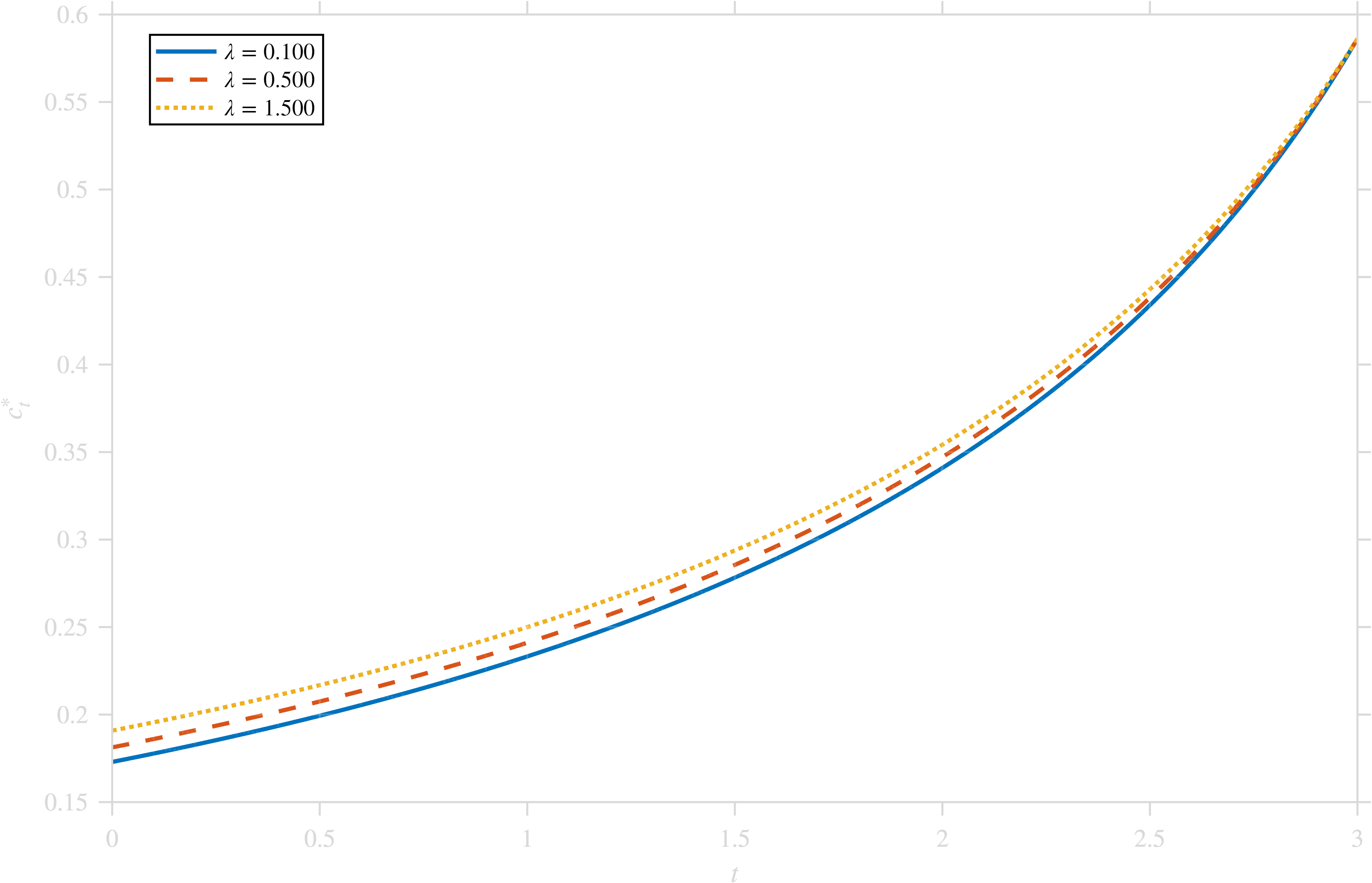
First, as illustrated in Figure 1, the consumption strategy ct∗c_{t}^{*} increases with λ\lambda, θ\theta, σ\sigma, and σ0\sigma^{0}. This behavior admits a natural economic interpretation. A higher jump intensity λ\lambda increases the exposure of future wealth to adverse jump shocks, making investment less attractive and inducing the agent to consume more in the present. A larger competition weight parameter θ\theta places greater weight on relative consumption performance, thereby strengthening the incentive for current consumption. In addition, higher values of the idiosyncratic volatility σ\sigma and the common volatility σ0\sigma_{0} increase uncertainty in future wealth accumulation, prompting the agent to shift consumption toward the present in response to the elevated level of market risk.
Refer to caption
Refer to caption
Refer to caption
Refer to caption
Figure 1: Mean field equilibrium strategy ct∗c_{t}^{*} with respect to λ\lambda, σ\sigma, σ0\sigma^{0}, and θ\theta
Refer to caption
Refer to caption
Refer to caption
Figure 2: Mean field equilibrium strategy ct∗c_{t}^{*} with respect to bb, γ\gamma, and ε\varepsilon

By contrast, Figure 2 shows that ct∗c_{t}^{*} decreases with bb, γ\gamma, and ε\varepsilon. These monotone relationships are also consistent with standard economic intuition. A larger value of bb corresponds to a higher expected return on the risky asset, making investment opportunities more attractive and thereby reducing the incentive for current consumption. Furthermore, a smaller γ\gamma corresponds to a higher degree of risk aversion. In this case, the agent adopts a more conservative investment strategy, which leads to a higher consumption rate. Finally, the effect of the terminal weight parameter ε\varepsilon is straightforward: A larger value of ε\varepsilon increases the importance of terminal wealth in the optimization objective and consequently lowers current consumption.

In particular, all the curves of ct∗c_{t}^{*} in Figures 1 and 2 are increasing over time. An intuitive explanation is that, in the earlier stage, the agent tends to preserve wealth to maintain future investment opportunities. As time passes, the additional gain from preserving wealth for future investment gradually diminishes, and the agent is therefore more willing to allocate wealth to current consumption.

Refer to caption
Figure 3: The effect of the terminal time TT on mean field equilibrium strategy ct0∗c_{t_{0}}^{*}

We now examine the effect of the investment horizon TT on the MFE consumption strategy ct∗c_{t}^{*}. As shown in Figure 3, for each fixed time t0t_{0}, the consumption level ct0∗c_{t_{0}}^{*} decreases as TT increases. A longer planning horizon increases the continuation value of retained wealth, thereby raising the opportunity cost of current consumption. As a result, the agent has a stronger incentive to save and consume less in the present.

Figure 4 further shows that changes in TT affect only the trajectory of ct∗c_{t}^{*}, while leaving the terminal value cT∗c_{T}^{*} unchanged. This property follows directly from the explicit expression for ct∗c_{t}^{*}. Indeed, by setting t=Tt=T, we obtain

cT∗=ε1γ−θ​γ−1.c_{T}^{*}=\varepsilon^{\frac{1}{\gamma-\theta\gamma-1}}.

Hence, cT∗c^{*}_{T} depends only on the model parameters and is independent of TT. Consequently, all curves in Figure 4 attain the same terminal value.

Refer to caption
Figure 4: Independence of mean field equilibrium strategy cT∗c^{*}_{T} from the terminal time TT

4 Approximate Nash equilibrium in the N-player game

Before constructing a uNu_{N}-Nash equilibrium for the NN-player game, we introduce an auxiliary control problem based on the representative agent model, which plays a key role in the construction of approximate Nash equilibrium strategies. The auxiliary control problem is given by

sup(πi,ci)∈𝒜iJ¯i​((πi,ci);(m∗,Γ∗))\displaystyle\sup_{(\pi^{i},c^{i})\in\mathcal{A}_{i}}\bar{J}_{i}((\pi^{i},c^{i});(m^{*},\Gamma^{*})) (29)
:=\displaystyle= sup(πi,ci)∈𝒜i𝔼​[∫0TU​(cti​Xti​(Γt∗​mt∗)−θi;γi)​𝑑t+εi​U​(XTi​(mT∗)−θi;γi)],\displaystyle\sup_{(\pi^{i},c^{i})\in\mathcal{A}_{i}}\mathbb{E}\left[\int_{0}^{T}U(c_{t}^{i}X_{t}^{i}(\Gamma^{*}_{t}m^{*}_{t})^{-\theta_{i}};\gamma_{i})dt+\varepsilon_{i}U(X_{T}^{i}(m^{*}_{T})^{-\theta_{i}};\gamma_{i})\right],

subject to

{d​Xti=(πti​bi−cti)​Xti​d​t+πti​Xti​σi​d​Wti+πti​Xti​σi0​d​Wt0−πti​Xt−i​d​Mti,d​mt∗=mt∗​[η​(π∗)−ct∗]​d​t+σ0​mt∗​π∗​d​Wt0,d​Γt∗=d​ct∗.\begin{cases}dX_{t}^{i}=\left(\pi_{t}^{i}b_{i}-c_{t}^{i}\right)X_{t}^{i}dt+\pi_{t}^{i}X_{t}^{i}\sigma_{i}dW_{t}^{i}+\pi_{t}^{i}X_{t}^{i}\sigma_{i}^{0}dW_{t}^{0}-\pi_{t}^{i}X_{t-}^{i}dM_{t}^{i},\\ dm_{t}^{*}=m_{t}^{*}[\eta\left(\pi^{*}\right)-c_{t}^{*}]dt+\sigma^{0}m_{t}^{*}\pi^{*}dW_{t}^{0},\\ d\Gamma_{t}^{*}=dc^{*}_{t}.\end{cases}

In this model, m∗=(mt∗)t∈[0,T]m^{*}=(m_{t}^{*})_{t\in[0,T]} and Γ∗=(Γt∗)t∈[0,T]\Gamma^{*}=(\Gamma_{t}^{*})_{t\in[0,T]} are the fixed point obtained in the limiting case, and π∗,c∗=(ct∗)t∈[0,T]\pi^{*},c^{*}=(c_{t}^{*})_{t\in[0,T]} are the deterministic MFE strategies. The following lemma provides the optimal strategy for the auxiliary control problem. Since the proof follows from the stochastic maximum principle and is similar to that of Theorem 1.6, we omit the details.

Lemma 4.1.

Let (π^i,c^i)∈𝒜i(\hat{\pi}^{i},\hat{c}^{i})\in\mathcal{A}_{i} be the optimal strategy of the auxiliary control problem, then for all t∈[0,T]t\in[0,T], π^ti=π^i\hat{\pi}^{i}_{t}=\hat{\pi}^{i} satisfies the following equation,

(γi−1)​(σi2+(σi0)2)​π^i−θi​γi​σi0​σ0​π∗−λi​((1−π^i)γi−1−1)+bi=0\displaystyle(\gamma_{i}-1)\left(\sigma_{i}^{2}+\left(\sigma_{i}^{0}\right)^{2}\right)\hat{\pi}^{i}-\theta_{i}\gamma_{i}\sigma_{i}^{0}\sigma^{0}\pi^{*}-\lambda_{i}\left(\left(1-\hat{\pi}^{i}\right)^{\gamma_{i}-1}-1\right)+b_{i}=0

and

c^ti={Ai​Bi​eAi​(t−T)Bi​(1−eAi​(t−T))+Ai,Ai≠0,Bi1+Bi​(T−t),Ai=0,\hat{c}_{t}^{i}=\begin{cases}\dfrac{A_{i}B_{i}e^{A_{i}(t-T)}}{B_{i}(1-e^{A_{i}(t-T)})+A_{i}},&A_{i}\neq 0,\\ \dfrac{B_{i}}{1+B_{i}(T-t)},&A_{i}=0,\end{cases}

where AiA_{i} and BiB_{i} are defined by

Ai=1γi−1​[ρ^+θi​γi​ργ−θ​γ−1],Bi=(εi​εθi​γiγ−θ​γ−1)1γi−1,\displaystyle A_{i}=\frac{1}{\gamma_{i}-1}[\hat{\rho}+\theta_{i}\gamma_{i}\frac{\rho}{\gamma-\theta\gamma-1}],B_{i}=\left(\varepsilon_{i}\varepsilon^{\frac{\theta_{i}\gamma_{i}}{\gamma-\theta\gamma-1}}\right)^{\frac{1}{\gamma_{i}-1}},

here

ρ^=\displaystyle\hat{\rho}= −(γi−1)​(bi+λi)​π^i+θi​γi​η​(π∗)+θi​γi​(γi−1)​σi0​σ0​π^i​π∗\displaystyle-(\gamma_{i}-1)(b_{i}+\lambda_{i})\hat{\pi}^{i}+\theta_{i}\gamma_{i}\eta(\pi^{*})+\theta_{i}\gamma_{i}\left(\gamma_{i}-1\right)\sigma^{0}_{i}\sigma^{0}\hat{\pi}^{i}\pi^{*}
−12​θi​γi​(θi​γi+1)​(σ0)2​(π∗)2−12​(γi−1)​(γi−2)​(σi2+(σi0)2)​(π^i)2\displaystyle-\frac{1}{2}\theta_{i}\gamma_{i}(\theta_{i}\gamma_{i}+1)\left(\sigma^{0}\right)^{2}\left(\pi^{*}\right)^{2}-\frac{1}{2}(\gamma_{i}-1)(\gamma_{i}-2)\left(\sigma_{i}^{2}+\left(\sigma_{i}^{0}\right)^{2}\right)\left(\hat{\pi}^{i}\right)^{2}
−[(1−π^i)γi−1−1]​λi.\displaystyle-\left[\left(1-\hat{\pi}^{i}\right)^{\gamma_{i}-1}-1\right]\lambda_{i}.

By Bo et al. [7, Lemma 4.2], there exists a unique solution π^i∈[D0,1−ϵ0]\hat{\pi}^{i}\in[D_{0},1-\epsilon_{0}]. We define this solution as π^i=ϕi​(ξ,ξi)\hat{\pi}^{i}=\phi_{i}(\xi,\xi^{i}), which only depends on parameters ξ\xi and ξi\xi^{i}. Analogously, we define c^ti=φi​(t,ξ,ξi)\hat{c}^{i}_{t}=\varphi_{i}(t,\xi,\xi^{i}).

We then construct optimal strategies for the system with NN agents and verify that these strategies constitute an approximate Nash equilibrium. For i=1,⋯,Ni=1,\cdots,N, we recall the objective functional (3) of agent ii:

Ji​((πi,ci),(𝝅,𝒄)−i)=𝔼​[∫0TU​(cti​Xti​(ct​Xt¯)−θi;γi)​𝑑t+εi​U​(XTi​XT¯−θi;γi)],J_{i}((\pi^{i},c^{i}),(\bm{\pi},\bm{c})^{-i})=\mathbb{E}\left[\int_{0}^{T}U(c_{t}^{i}X_{t}^{i}(\overline{c_{t}X_{t}})^{-\theta_{i}};\gamma_{i})dt+\varepsilon_{i}U(X_{T}^{i}\overline{X_{T}}^{-\theta_{i}};\gamma_{i})\right], (30)

where (𝝅,𝒄)−i:=((π1,c1),…,(πi−1,ci−1),(πi+1,ci+1),…,(πN,cN))(\bm{\pi},\bm{c})^{-i}:=\left((\pi^{1},c^{1}),\ldots,(\pi^{i-1},c^{i-1}),(\pi^{i+1},c^{i+1}),\ldots,(\pi^{N},c^{N})\right). Subsequently, for i=1,⋯,Ni=1,\cdots,N, we consider a strategy of agent ii

π∗,i=ϕi​(ξ,ξi),ct∗,i=φi​(t,ξ,ξi),t∈[0,T].\pi^{*,i}=\phi_{i}(\xi,\xi^{i}),\ c^{*,i}_{t}=\varphi_{i}(t,\xi,\xi^{i}),\qquad t\in[0,T]. (31)

Then the SDE system for agent ii under strategy π∗,i\pi^{*,i} and ct∗,ic^{*,i}_{t} is given by

d​Xt∗,i=(π∗,i​bi−ct∗,i)​Xt∗,i​d​t+π∗,i​Xt∗,i​σi​d​Wti+π∗,i​Xt∗,i​σi0​d​Wt0−π∗,i​Xt−∗,i​d​Mti.\displaystyle dX_{t}^{*,i}=\left(\pi^{*,i}b_{i}-c^{*,i}_{t}\right)X_{t}^{*,i}dt+\pi^{*,i}X_{t}^{*,i}\sigma_{i}dW_{t}^{i}+\pi^{*,i}X_{t}^{*,i}\sigma_{i}^{0}dW_{t}^{0}-\pi^{*,i}X_{t-}^{*,i}dM_{t}^{i}. (32)

To prove Theorem 1.7, we first establish the following lemma.

Lemma 4.2.

Let Assumption 1.4 hold. Then, for any p∈ℝp\in\mathbb{R}, there exist two constants Cp∗,1,Cp∗,2C_{p}^{*,1},C_{p}^{*,2} such that, for t∈[0,T]t\in[0,T],

𝔼​[(mt∗)p]⩽Cp∗,1,𝔼​[(Γt∗)p]⩽Cp∗,2.\mathbb{E}\left[\left(m^{*}_{t}\right)^{p}\right]\leqslant C_{p}^{*,1},\quad\mathbb{E}\left[\left(\Gamma^{*}_{t}\right)^{p}\right]\leqslant C_{p}^{*,2}. (33)
Proof.

We first discuss the boundedness of π∗\pi^{*} and ct∗c_{t}^{*} for t∈[0,T]t\in[0,T]. It follows from the proof of Theorem 1.6 that π∗∈(0,1−ϵ0]\pi^{*}\in(0,1-\epsilon_{0}], and that c∗c^{*} is continuous and strictly positive on [0,T][0,T]. Hence, c∗c^{*} is bounded away from zero and infinity on [0,T][0,T]. Therefore, for every p∈ℝp\in\mathbb{R},

𝔼​[(Γt∗)p]=(ct∗)p⩽Cp∗,2.\mathbb{E}\left[\left(\Gamma_{t}^{*}\right)^{p}\right]=\left(c_{t}^{*}\right)^{p}\leqslant C_{p}^{*,2}.

We next establish the boundedness of 𝔼​[(mt∗)p]\mathbb{E}\left[\left(m^{*}_{t}\right)^{p}\right]. By (8),

𝔼​[(mt∗)p]=𝔼​[x0p​exp⁡{p​∫0t(η​(π∗)−cs∗−12​(σ0​π∗)2)​𝑑s+p​∫0tσ0​π∗​𝑑Ws0}].\mathbb{E}\left[\left(m^{*}_{t}\right)^{p}\right]=\mathbb{E}\left[x_{0}^{p}\exp\left\{p\int_{0}^{t}\left(\eta\left(\pi^{*}\right)-c_{s}^{*}-\frac{1}{2}\left(\sigma^{0}\pi^{*}\right)^{2}\right)ds+p\int_{0}^{t}\sigma^{0}\pi^{*}dW_{s}^{0}\right\}\right]. (34)

Let

αs=η​(π∗)−cs∗−12​(σ0​π∗)2,β=σ0​π∗.\alpha_{s}=\eta\left(\pi^{*}\right)-c_{s}^{*}-\frac{1}{2}\left(\sigma^{0}\pi^{*}\right)^{2},\qquad\beta=\sigma^{0}\pi^{*}.

By Assumption 1.4, there exist constants L1L_{1} and L2L_{2} such that, for all s∈[0,T]s\in[0,T],

|αs|⩽L1,|β|⩽L2.|\alpha_{s}|\leqslant L_{1},\qquad|\beta|\leqslant L_{2}. (35)

Under the initial probability measure ℙ\mathbb{P}, consider the process defined by

Zt=exp⁡{p​∫0tβ​𝑑Ws0−p22​∫0tβ2​𝑑s}.Z_{t}=\exp\left\{p\int_{0}^{t}\beta dW_{s}^{0}-\frac{p^{2}}{2}\int_{0}^{t}\beta^{2}ds\right\}. (36)

From the Novikov condition, namely that

𝔼​[exp⁡{12​∫0Tp2​β2​𝑑s}]⩽exp⁡{12​p2​L22​T}<∞,\mathbb{E}\left[\exp\left\{\frac{1}{2}\int_{0}^{T}p^{2}\beta^{2}ds\right\}\right]\leqslant\exp\left\{\frac{1}{2}p^{2}L_{2}^{2}T\right\}<\infty,

it follows that ZtZ_{t} is a martingale with 𝔼​[Zt]=1\mathbb{E}[Z_{t}]=1. Define a new probability measure ℚ∼ℙ\mathbb{Q}\sim\mathbb{P} by

d​ℚd​ℙ|𝒢t=Zt.\frac{d\mathbb{Q}}{d\mathbb{P}}\bigg|_{\mathcal{G}_{t}}=Z_{t}.

Applying the change of measure, we have

𝔼​[exp⁡{p​∫0tβ​𝑑Ws0}]=𝔼ℚ​[exp⁡{p22​∫0tβ2​𝑑s}]⩽exp⁡{12​p2​L22​T}.\displaystyle\mathbb{E}\left[\exp\left\{p\int_{0}^{t}\beta dW_{s}^{0}\right\}\right]=\mathbb{E}^{\mathbb{Q}}\left[\exp\left\{\frac{p^{2}}{2}\int_{0}^{t}\beta^{2}ds\right\}\right]\leqslant\exp\left\{\frac{1}{2}p^{2}L_{2}^{2}T\right\}. (37)

Substituting (35) and (37) into (34), we obtain

𝔼​[(mt∗)p]⩽x0p​exp⁡{|p|​L1​T+12​p2​L22​T}:=Cp∗,1.\mathbb{E}\left[\left(m^{*}_{t}\right)^{p}\right]\leqslant x_{0}^{p}\exp\left\{|p|L_{1}T+\frac{1}{2}p^{2}L_{2}^{2}T\right\}:=C_{p}^{*,1}.

This completes the proof of the lemma. ∎

Lemma 4.3.

Let Assumption 1.4 hold. Then, for any q∈ℝq\in\mathbb{R}, there exist deterministic constants Cq∗,1C_{q}^{*,1} and C∗,2C^{*,2}, independent of NN and ii, such that, for every i=1,…,Ni=1,\ldots,N and every admissible pair (πi,ci)∈𝒜i(\pi^{i},c^{i})\in\mathcal{A}_{i},

supt∈[0,T]𝔼​[|ct∗,i​Xt∗,i|q]⩽Cq∗,1,𝔼​[∫0Tcti​Xti​𝑑t]⩽C∗,2.\sup_{t\in[0,T]}\mathbb{E}\left[\left|c_{t}^{*,i}X_{t}^{*,i}\right|^{q}\right]\leqslant C_{q}^{*,1},\qquad\mathbb{E}\left[\int_{0}^{T}c_{t}^{i}X_{t}^{i}\,dt\right]\leqslant C^{*,2}. (38)
Proof.

We first establish the first inequality in the lemma. By Lemma 4.1, ct∗,i=c^tic_{t}^{*,i}=\hat{c}_{t}^{i} is given explicitly in terms of AiA_{i} and BiB_{i}. By Assumption 1.4 and the explicit forms of AiA_{i} and BiB_{i}, there exist constants 0<A¯<∞0<\bar{A}<\infty and 0<B¯⩽B¯<∞0<\underline{B}\leqslant\bar{B}<\infty, independent of NN and ii, such that

|Ai|⩽A¯,B¯⩽Bi⩽B¯.|A_{i}|\leqslant\bar{A},\qquad\underline{B}\leqslant B_{i}\leqslant\bar{B}.

Hence, from the explicit formula of c^ti\hat{c}_{t}^{i}, the family {ct∗,i}i,N\{c_{t}^{*,i}\}_{i,N} is uniformly bounded away from zero and infinity on [0,T][0,T]. Consequently, for every q∈ℝq\in\mathbb{R}, there exists a constant L~q∗,1\tilde{L}_{q}^{*,1}, independent of NN and ii, such that

supt∈[0,T]|ct∗,i|q⩽L~q∗,1,i=1,…,N.\sup_{t\in[0,T]}\left|c_{t}^{*,i}\right|^{q}\leqslant\tilde{L}_{q}^{*,1},\qquad i=1,\ldots,N.

Therefore, it remains to show that, for every q∈ℝq\in\mathbb{R}, there exists a constant L~q∗,2\tilde{L}_{q}^{*,2}, independent of NN and ii, such that

supt∈[0,T]𝔼​[|Xt∗,i|q]⩽L~q∗,2,i=1,…,N.\sup_{t\in[0,T]}\mathbb{E}\left[\left|X_{t}^{*,i}\right|^{q}\right]\leqslant\tilde{L}_{q}^{*,2},\qquad i=1,\ldots,N.

Recalling that the wealth process Xt∗,iX^{*,i}_{t} satisfies (32), an application of Itô’s formula yields

(Xt∗,i)q=\displaystyle(X_{t}^{*,i})^{q}= (x0i)qexp{q∫0t[π∗,i(bi+λi)−cs∗,i−12(π∗,i)2(σi2+(σi0)2)]ds\displaystyle(x_{0}^{i})^{q}\exp\left\{q\int_{0}^{t}\left[\pi^{*,i}(b_{i}+\lambda_{i})-c_{s}^{*,i}-\frac{1}{2}(\pi^{*,i})^{2}(\sigma_{i}^{2}+(\sigma_{i}^{0})^{2})\right]ds\right.
+q∫0tπ∗,i(σidWsi+σi0dWs0)+q∫0tln(1−π∗,i)dNsi}.\displaystyle\left.+q\int_{0}^{t}\pi^{*,i}(\sigma_{i}dW_{s}^{i}+\sigma_{i}^{0}dW_{s}^{0})+q\int_{0}^{t}\ln(1-\pi^{*,i})\,dN_{s}^{i}\right\}.

Similar to the proof of Lemma 4.2, we define the following process

Z~t=exp\displaystyle\widetilde{Z}_{t}=\exp {q∫0tπ∗,i(σidWsi+σi0dWs0)−12q2∫0t(π∗,i)2(σi2+(σi0)2)ds\displaystyle\left\{q\int_{0}^{t}\pi^{*,i}(\sigma_{i}dW_{s}^{i}+\sigma_{i}^{0}dW_{s}^{0})-\frac{1}{2}q^{2}\int_{0}^{t}(\pi^{*,i})^{2}(\sigma_{i}^{2}+(\sigma_{i}^{0})^{2})ds\right.
+q∫0tln(1−π∗,i)dNsi+∫0t[1−(1−π∗,i)q]λids}.\displaystyle\left.+q\int_{0}^{t}\ln(1-\pi^{*,i})dN_{s}^{i}+\int_{0}^{t}[1-(1-\pi^{*,i})^{q}]\lambda_{i}ds\right\}.

By the Novikov condition for Lévy processes, we can verify that (Z~t)t∈[0,T](\widetilde{Z}_{t})_{t\in[0,T]} is a martingale and that 𝔼​[Z~t]=1\mathbb{E}[\widetilde{Z}_{t}]=1. Define a new probability measure ℚ~∼ℙ\widetilde{\mathbb{Q}}\sim\mathbb{P} by

d​ℚ~d​ℙ∣𝒢t=Z~t,t∈[0,T].\frac{d\widetilde{\mathbb{Q}}}{d\mathbb{P}}\mid_{\mathcal{G}_{t}}=\widetilde{Z}_{t},\quad t\in[0,T].

Observe that

𝔼​[(Xt∗,i)q]\displaystyle\mathbb{E}[(X_{t}^{*,i})^{q}] =(x0i)q𝔼ℚ~[exp{∫0t[qπ∗,i(bi+λi)−qcs∗,i\displaystyle=(x_{0}^{i})^{q}\mathbb{E}^{\widetilde{\mathbb{Q}}}\left[\exp\left\{\int_{0}^{t}\left[q\pi^{*,i}(b_{i}+\lambda_{i})-qc_{s}^{*,i}\right.\right.\right.
+12q(q−1)(π∗,i)2(σi2+(σi0)2)+λi((1−π∗,i)q−1)]ds}].\displaystyle\qquad\qquad\left.\left.\left.+\frac{1}{2}q(q-1)(\pi^{*,i})^{2}(\sigma_{i}^{2}+(\sigma_{i}^{0})^{2})+\lambda_{i}((1-\pi^{*,i})^{q}-1)\right]ds\right\}\right].

Since ξi\xi^{i}, π∗,i\pi^{*,i}, and cs∗,ic_{s}^{*,i} are uniformly bounded, it follows that, for every q∈ℝq\in\mathbb{R},

supt∈[0,T]𝔼​[|Xt∗,i|q]⩽L~q∗,2,i=1,…,N.\sup_{t\in[0,T]}\mathbb{E}\left[\left|X_{t}^{*,i}\right|^{q}\right]\leqslant\tilde{L}_{q}^{*,2},\qquad i=1,\ldots,N. (39)

Hence, we obtain

supt∈[0,T]𝔼​[|ct∗,i​Xt∗,i|q]⩽supt∈[0,T]|ct∗,i|q​supt∈[0,T]𝔼​[|Xt∗,i|q]⩽Cq∗,1.\sup_{t\in[0,T]}\mathbb{E}\left[\left|c^{*,i}_{t}X^{*,i}_{t}\right|^{q}\right]\leqslant\sup_{t\in[0,T]}\left|c^{*,i}_{t}\right|^{q}\sup_{t\in[0,T]}\mathbb{E}\left[\left|X^{*,i}_{t}\right|^{q}\right]\leqslant C_{q}^{*,1}.

Next, we prove the second inequality. Let (πi,ci)∈𝒜i(\pi^{i},c^{i})\in\mathcal{A}_{i} be arbitrary. Set

Ati:=∫0tcsi​𝑑s,t∈[0,T].A_{t}^{i}:=\int_{0}^{t}c_{s}^{i}\,ds,\qquad t\in[0,T].

By Definition 1.1, ATi<∞A_{T}^{i}<\infty, ℙ\mathbb{P}-a.s. The wealth process can be written as

Xti=Rti​e−Ati,X_{t}^{i}=R_{t}^{i}e^{-A_{t}^{i}},

where

Rti=\displaystyle R_{t}^{i}= x0iexp{∫0t[πsi(bi+λi)−12(πsi)2(σi2+(σi0)2)]ds\displaystyle x_{0}^{i}\exp\Bigg\{\int_{0}^{t}\left[\pi_{s}^{i}(b_{i}+\lambda_{i})-\frac{1}{2}(\pi_{s}^{i})^{2}\left(\sigma_{i}^{2}+(\sigma_{i}^{0})^{2}\right)\right]ds
+∫0tπsi(σidWsi+σi0dWs0)+∫0tln(1−πsi)dNsi}.\displaystyle\quad+\int_{0}^{t}\pi_{s}^{i}\left(\sigma_{i}dW_{s}^{i}+\sigma_{i}^{0}dW_{s}^{0}\right)+\int_{0}^{t}\ln(1-\pi_{s}^{i})\,dN_{s}^{i}\Bigg\}.

Using the same argument as in the proof of the boundedness estimate (39), we obtain, for any q^>0\hat{q}>0 and any i=1,…,Ni=1,\ldots,N,

supt∈[0,T]𝔼​[(Xti)q^]⩽supt∈[0,T]𝔼​[(Rti)q^]⩽L~q^,\sup_{t\in[0,T]}\mathbb{E}\left[\left(X_{t}^{i}\right)^{\hat{q}}\right]\leqslant\sup_{t\in[0,T]}\mathbb{E}\left[\left(R_{t}^{i}\right)^{\hat{q}}\right]\leqslant\tilde{L}_{\hat{q}}, (40)

where L~q^\tilde{L}_{\hat{q}} is a deterministic constant independent of NN, ii, and the admissible pair (πi,ci)(\pi^{i},c^{i}). Integrating the wealth equation (2) and then taking expectations, we obtain

𝔼​[∫0Tcti​Xti​𝑑t]=x0i+𝔼​[∫0Tπti​bi​Xti​𝑑t]−𝔼​[XTi].\mathbb{E}\left[\int_{0}^{T}c_{t}^{i}X_{t}^{i}\,dt\right]=x_{0}^{i}+\mathbb{E}\left[\int_{0}^{T}\pi_{t}^{i}b_{i}X_{t}^{i}\,dt\right]-\mathbb{E}[X_{T}^{i}].

Since XTi≥0X_{T}^{i}\geq 0, πi\pi^{i} is bounded, and bib_{i} is uniformly bounded under Assumption 1.4, it follows from (40) with q^=1\hat{q}=1 that

𝔼​[∫0Tcti​Xti​𝑑t]\displaystyle\mathbb{E}\left[\int_{0}^{T}c_{t}^{i}X_{t}^{i}\,dt\right] ≤x0i+K​supt∈[0,T]𝔼​[Xti]\displaystyle\leq x_{0}^{i}+K\sup_{t\in[0,T]}\mathbb{E}[X_{t}^{i}]
≤C∗,2.\displaystyle\leq C^{*,2}.

Here and throughout the rest of the paper, KK denotes a deterministic constant independent of NN, ii, and the admissible pair (πi,ci)∈𝒜i(\pi^{i},c^{i})\in\mathcal{A}_{i}, whose value may change from line to line. This completes the proof of the lemma. ∎

Remark 4.4.

By Hölder’s inequality, Lemma 4.3 yields the following consequence: for any a∈(0,1)a\in(0,1) and any admissible control (πi,ci)∈𝒜i(\pi^{i},c^{i})\in\mathcal{A}_{i}, there exists a deterministic constant Ca∗C_{a}^{*}, independent of NN, ii, and (πi,ci)(\pi^{i},c^{i}), such that, for every i=1,…,Ni=1,\ldots,N,

𝔼​[∫0T(cti​Xti)a​𝑑t]\displaystyle\mathbb{E}\left[\int_{0}^{T}(c_{t}^{i}X_{t}^{i})^{a}\,dt\right] ⩽(𝔼​[∫0Tcti​Xti​𝑑t])a​(𝔼​[∫0T1​𝑑t])1−a⩽Ca∗.\displaystyle\leqslant\left(\mathbb{E}\left[\int_{0}^{T}c_{t}^{i}X_{t}^{i}\,dt\right]\right)^{a}\left(\mathbb{E}\left[\int_{0}^{T}1\,dt\right]\right)^{1-a}\leqslant C_{a}^{*}.
Lemma 4.5.

Let Assumption 1.4 hold. Then, for any n>0n>0, the following assertions hold: for each t∈[0,T]t\in[0,T],

limN→∞𝔼​[|Xt∗¯−mt∗|n]=0,\lim_{N\to\infty}\mathbb{E}\left[\left|\overline{X_{t}^{*}}-m_{t}^{*}\right|^{n}\right]=0,

and

limN→∞𝔼​[∫0T|mt∗​Γt∗−ct∗¯​Xt∗¯|n​𝑑t]=0.\lim_{N\to\infty}\mathbb{E}\left[\int_{0}^{T}\left|m_{t}^{*}\Gamma_{t}^{*}-\overline{c_{t}^{*}}\,\overline{X_{t}^{*}}\right|^{n}\,dt\right]=0.

Here, Xt∗¯=(∏j=1NXt∗,j)1N,ct∗¯=(∏j=1Nct∗,j)1N\overline{X_{t}^{*}}=\left(\prod_{j=1}^{N}X^{*,j}_{t}\right)^{\frac{1}{N}},\overline{c_{t}^{*}}=\left(\prod_{j=1}^{N}c^{*,j}_{t}\right)^{\frac{1}{N}}, and mt∗,Γt∗m_{t}^{*},\Gamma_{t}^{*} are the limiting processes given in Theorem 1.6.

Proof.

For i=1,⋯,Ni=1,\cdots,N, set Yt∗,i:=ln⁡Xt∗,iY_{t}^{*,i}:=\ln X_{t}^{*,i}. Then

Yt∗¯:=1N​∑i=1NYt∗,i=1N​∑i=1Nln⁡Xt∗,i=ln⁡Xt∗¯,\overline{Y_{t}^{*}}:=\frac{1}{N}\sum_{i=1}^{N}Y_{t}^{*,i}=\frac{1}{N}\sum_{i=1}^{N}\ln X_{t}^{*,i}=\ln\overline{X_{t}^{*}},

We first prove that, as N→∞N\to\infty,

𝔼​[|Xt∗¯−mt∗|n]=𝔼​[|eYt∗¯−eln⁡mt∗|n]→0.\mathbb{E}\left[\left|\overline{X_{t}^{*}}-m_{t}^{*}\right|^{n}\right]=\mathbb{E}\left[\left|e^{\overline{Y_{t}^{*}}}-e^{\ln m^{*}_{t}}\right|^{n}\right]\to 0.

By Lemmas 4.2 and 4.3, for any k>0k>0,

𝔼​[(Xt∗¯)k]⩽∏i=1N{𝔼​[(Xt∗,i)k]}1N⩽K,𝔼​[(mt∗)k]⩽K.\mathbb{E}\left[\left(\overline{X_{t}^{*}}\right)^{k}\right]\leqslant\prod_{i=1}^{N}\left\{\mathbb{E}\left[(X_{t}^{*,i})^{k}\right]\right\}^{\frac{1}{N}}\leqslant K,\qquad\mathbb{E}\left[(m_{t}^{*})^{k}\right]\leqslant K.

Hence, for any κ>0\kappa>0,

supN⩾1𝔼​[|Xt∗¯−mt∗|n​(1+κ)]⩽Cn,κ​supN⩾1𝔼​[|Xt∗¯|n​(1+κ)+|mt∗|n​(1+κ)]⩽K.\sup_{N\geqslant 1}\mathbb{E}\left[\left|\overline{X_{t}^{*}}-m_{t}^{*}\right|^{n(1+\kappa)}\right]\leqslant C_{n,\kappa}\sup_{N\geqslant 1}\mathbb{E}\left[|\overline{X_{t}^{*}}|^{n(1+\kappa)}+|m_{t}^{*}|^{n(1+\kappa)}\right]\leqslant K.

where Cn,κC_{n,\kappa} is a constant depending only on n,κn,\kappa. Therefore, {|Xt∗¯−mt∗|n}N⩾1\Big\{\big|\overline{X_{t}^{*}}-m_{t}^{*}\big|^{n}\Big\}_{N\geqslant 1} is uniformly integrable. By Vitali’s convergence theorem, it is enough to prove that

eYt∗¯→eln⁡mt∗in probability.e^{\overline{Y_{t}^{*}}}\to e^{\ln m^{*}_{t}}\qquad\text{in probability}.

Since the exponential function is continuous, by the continuous mapping theorem it suffices to show that

Yt∗¯→ln⁡mt∗in probability.\overline{Y_{t}^{*}}\to\ln m_{t}^{*}\qquad\text{in probability}.

Applying Itô’s formula to Yt∗,i=ln⁡Xt∗,iY_{t}^{*,i}=\ln X_{t}^{*,i}, we obtain

Yt∗,i=\displaystyle Y_{t}^{*,i}= ln⁡x0i+∫0t[π∗,i​(bi+λi)−cs∗,i−12​(π∗,i)2​(σi2+(σi0)2)+λi​ln⁡(1−π∗,i)]​𝑑s\displaystyle\ln x_{0}^{i}+\int_{0}^{t}\left[\pi^{*,i}(b_{i}+\lambda_{i})-c_{s}^{*,i}-\frac{1}{2}(\pi^{*,i})^{2}\left(\sigma_{i}^{2}+(\sigma_{i}^{0})^{2}\right)+\lambda_{i}\ln(1-\pi^{*,i})\right]ds
+∫0tπ∗,i​σi​𝑑Wsi+∫0tπ∗,i​σi0​𝑑Ws0+∫0tln⁡(1−π∗,i)​𝑑Msi.\displaystyle+\int_{0}^{t}\pi^{*,i}\sigma_{i}dW_{s}^{i}+\int_{0}^{t}\pi^{*,i}\sigma_{i}^{0}dW_{s}^{0}+\int_{0}^{t}\ln(1-\pi^{*,i})dM_{s}^{i}.

On the other hand, by (8) in Theorem 1.6,

ln⁡mt∗=\displaystyle\ln m_{t}^{*}= ln⁡x0+∫0t[π∗​(b+λ)−cs∗−12​(π∗)2​(σ2+(σ0)2)+λ​ln⁡(1−π∗)]​𝑑s\displaystyle\ln x_{0}+\int_{0}^{t}\left[\pi^{*}(b+\lambda)-c_{s}^{*}-\frac{1}{2}(\pi^{*})^{2}\left(\sigma^{2}+(\sigma^{0})^{2}\right)+\lambda\ln(1-\pi^{*})\right]ds
+∫0tπ∗​σ0​𝑑Ws0.\displaystyle+\int_{0}^{t}\pi^{*}\sigma^{0}dW_{s}^{0}.

Define

μt∗¯:=1N​∑i=1N𝔼​[Yt∗,i∣ℱt0].\displaystyle\overline{\mu_{t}^{*}}=\frac{1}{N}\sum_{i=1}^{N}\mathbb{E}[Y_{t}^{*,i}\mid\mathcal{F}_{t}^{0}].

Then

Yt∗¯−ln⁡mt∗=(Yt∗¯−μt∗¯)+(μt∗¯−ln⁡mt∗).\overline{Y_{t}^{*}}-\ln m_{t}^{*}=\left(\overline{Y_{t}^{*}}-\overline{\mu_{t}^{*}}\right)+\left(\overline{\mu_{t}^{*}}-\ln m_{t}^{*}\right). (41)

We first estimate the first term. From the independence of (W1,…,WN)(W^{1},\dots,W^{N}) and (M1,…,MN)(M^{1},\dots,M^{N}), we have

𝔼​[|Yt∗¯−μt∗¯|2]\displaystyle\mathbb{E}\left[\left|\overline{Y_{t}^{*}}-\overline{\mu_{t}^{*}}\right|^{2}\right] =1N2𝔼[|∑i=1N(Yt∗,i−𝔼[Yt∗,i∣ℱt0])|2]\displaystyle=\frac{1}{N^{2}}\mathbb{E}\left[\left|\sum_{i=1}^{N}\left(Y_{t}^{*,i}-\mathbb{E}[Y_{t}^{*,i}\mid\mathcal{F}_{t}^{0}]\right)\right|^{2}\right]
=1N2∑i=1N𝔼[(∫0tπ∗,iσidWsi)2+(∫0tln(1−π∗,i)dMsi)2\displaystyle=\frac{1}{N^{2}}\sum_{i=1}^{N}\mathbb{E}\left[\left(\int_{0}^{t}\pi^{*,i}\sigma_{i}dW_{s}^{i}\right)^{2}+\left(\int_{0}^{t}\ln(1-\pi^{*,i})dM_{s}^{i}\right)^{2}\right.
+2(∫0tπ∗,iσidWsi)(∫0tln(1−π∗,i)dMsi)].\displaystyle\qquad\qquad\,\,\left.+2\left(\int_{0}^{t}\pi^{*,i}\sigma_{i}dW_{s}^{i}\right)\left(\int_{0}^{t}\ln(1-\pi^{*,i})dM_{s}^{i}\right)\right].

Using Itô’s isometry and the isometry for compensated Poisson integrals, we get

𝔼​[|Yt∗¯−μt∗¯|2]⩽2N2​∑i=1N𝔼​{∫0t[(π∗,i)2​σi2+λi​(ln⁡(1−π∗,i))2]​𝑑s}⩽KN.\displaystyle\mathbb{E}\left[\left|\overline{Y_{t}^{*}}-\overline{\mu_{t}^{*}}\right|^{2}\right]\leqslant\frac{2}{N^{2}}\sum_{i=1}^{N}\mathbb{E}\left\{\int_{0}^{t}\left[(\pi^{*,i})^{2}\sigma_{i}^{2}+\lambda_{i}(\ln(1-\pi^{*,i}))^{2}\right]ds\right\}\leqslant\frac{K}{N}.

Consequently,

𝔼​[|Yt∗¯−μt∗¯|2]→0as ​N→∞.\mathbb{E}\left[\left|\overline{Y_{t}^{*}}-\overline{\mu_{t}^{*}}\right|^{2}\right]\to 0\qquad\text{as }N\to\infty. (42)

We next analyze the second term in (41) . Write

μt∗¯−ln⁡mt∗=AN+∫0tBsN​𝑑s+∫0tCsN​𝑑Ws0,\overline{\mu_{t}^{*}}-\ln m_{t}^{*}=A^{N}+\int_{0}^{t}B_{s}^{N}ds+\int_{0}^{t}C_{s}^{N}dW_{s}^{0},

where

{AN:=1N​∑i=1Nln⁡x0i−ln⁡x0,BsN:=1N​∑i=1N[π∗,i​(bi+λi)−cs∗,i−12​(π∗,i)2​(σi2+(σi0)2)+λi​ln⁡(1−π∗,i)]−[π∗​(b+λ)−cs∗−12​(π∗)2​(σ2+(σ0)2)+λ​ln⁡(1−π∗)],CsN:=1N​∑i=1Nπ∗,i​σi0−π∗​σ0.\left\{\begin{aligned} &A^{N}:=\frac{1}{N}\sum_{i=1}^{N}\ln x_{0}^{i}-\ln x_{0},\\ &B_{s}^{N}:=\frac{1}{N}\sum_{i=1}^{N}\left[\pi^{*,i}(b_{i}+\lambda_{i})-c_{s}^{*,i}-\frac{1}{2}(\pi^{*,i})^{2}\left(\sigma_{i}^{2}+(\sigma_{i}^{0})^{2}\right)+\lambda_{i}\ln(1-\pi^{*,i})\right]\\ &\qquad-\left[\pi^{*}(b+\lambda)-c_{s}^{*}-\frac{1}{2}(\pi^{*})^{2}\left(\sigma^{2}+(\sigma^{0})^{2}\right)+\lambda\ln(1-\pi^{*})\right],\\ &C_{s}^{N}:=\frac{1}{N}\sum_{i=1}^{N}\pi^{*,i}\sigma_{i}^{0}-\pi^{*}\sigma^{0}.\end{aligned}\right.

By Assumption 1.4, for any bounded continuous function ff, we have

1N​∑i=1Nf​(ξi)=∫𝒪f​(ζ)​𝑑ν0N→∫𝒪f​(ζ)​𝑑ν0=f​(ξ).\displaystyle\frac{1}{N}\sum_{i=1}^{N}f(\xi^{i})=\int_{\mathcal{O}}f(\zeta)d\nu_{0}^{N}\to\int_{\mathcal{O}}f(\zeta)d\nu_{0}=f(\xi). (43)

For ζ=(xζ,λζ,bζ,σζ,σζ0,εζ,γζ,θζ)∈𝒪\zeta=(x_{\zeta},\lambda_{\zeta},b_{\zeta},\sigma_{\zeta},\sigma^{0}_{\zeta},\varepsilon_{\zeta},\gamma_{\zeta},\theta_{\zeta})\in\mathcal{O}, ln⁡xζ\ln x_{\zeta} is a bounded continuous function. Therefore, by (43), we have

1N​∑i=1Nln⁡x0i→ln⁡x0as ​N→∞,\frac{1}{N}\sum_{i=1}^{N}\ln x_{0}^{i}\to\ln x_{0}\qquad\text{as }N\to\infty,

that is,

AN→0as ​N→∞.A^{N}\to 0\qquad\text{as }N\to\infty.

We now consider CsNC_{s}^{N}, fix s∈[0,T]s\in[0,T], let Φ​(ζ)\Phi(\zeta) denote the solution on [D0,1−ϵ0][D_{0},1-\epsilon_{0}] of the equation defining as following:

G​(x,ζ)=(γζ−1)​(σζ2+(σζ0)2)​x−θζ​γζ​σζ0​σ0​π∗−λζ​((1−x)γζ−1−1)+bζ=0.G(x,\zeta)=(\gamma_{\zeta}-1)\left(\sigma_{\zeta}^{2}+\left(\sigma_{\zeta}^{0}\right)^{2}\right)x-\theta_{\zeta}\gamma_{\zeta}\sigma_{\zeta}^{0}\sigma^{0}\pi^{*}-\lambda_{\zeta}\left(\left(1-x\right)^{\gamma_{\zeta}-1}-1\right)+b_{\zeta}=0.

Then, by uniqueness of the solution,

π∗,i=Φ​(ξi),π∗=Φ​(ξ).\pi^{*,i}=\Phi(\xi^{i}),\qquad\pi^{*}=\Phi(\xi).

We claim that Φ​(ζ)\Phi(\zeta) is continuous in ζ\zeta. Indeed, G​(x,ζ)G(x,\zeta) is continuous in (x,ζ)(x,\zeta). Let {ζn}n≥1⊂𝒪\{\zeta_{n}\}_{n\geq 1}\subset\mathcal{O} satisfy ζn→ζ\zeta_{n}\to\zeta, and define xn:=Φ​(ζn)x_{n}:=\Phi(\zeta_{n}). Since {xn}n≥1⊂[D0,1−ϵ0]\{x_{n}\}_{n\geq 1}\subset[D_{0},1-\epsilon_{0}] is bounded, there exists a subsequence {xnk}k≥1\{x_{n_{k}}\}_{k\geq 1} such that

xnk→x¯∈[D0,1−ϵ0].x_{n_{k}}\to\bar{x}\in[D_{0},1-\epsilon_{0}].

Using G​(xnk,ζnk)=0G(x_{n_{k}},\zeta_{n_{k}})=0 and the continuity of GG, we obtain G​(x¯,ζ)=0G(\bar{x},\zeta)=0. By uniqueness, x¯=Φ​(ζ)\bar{x}=\Phi(\zeta). Hence every convergent subsequence of {xn}n≥1\{x_{n}\}_{n\geq 1} has the same limit Φ​(ζ)\Phi(\zeta), and therefore

Φ​(ζn)→Φ​(ζ).\Phi(\zeta_{n})\to\Phi(\zeta).

Thus, Φ\Phi is continuous on 𝒪\mathcal{O}. Clearly, Φ​(ζ)​σζ0\Phi(\zeta)\sigma_{\zeta}^{0} is a bounded continuous function. Therefore, by (43), as N→∞N\to\infty,

1N​∑i=1Nπ∗,i​σi0=1N​∑i=1NΦ​(ξi)​σi0→Φ​(ξ)​σ0=π∗​σ0.\frac{1}{N}\sum_{i=1}^{N}\pi^{*,i}\sigma_{i}^{0}=\frac{1}{N}\sum_{i=1}^{N}\Phi(\xi^{i})\sigma_{i}^{0}\to\Phi(\xi)\sigma^{0}=\pi^{*}\sigma^{0}.

That is,

CsN→0as ​N→∞.C_{s}^{N}\to 0\qquad\text{as }N\to\infty.

Next we prove that

BsN→0as ​N→∞.B_{s}^{N}\to 0\qquad\text{as }N\to\infty.

For fixed s∈[0,T]s\in[0,T], denote Ψs​(ζ)\Psi_{s}(\zeta) as follows:

Ψs(ζ)={A​(ζ)​B​(ζ)​eA​(ζ)​(s−T)B​(ζ)​(1−eA​(ζ)​(s−T))+A​(ζ)A​(ζ)≠0,B​(ζ)1+B​(ζ)​(T−s)A​(ζ)=0,\Psi_{s}(\zeta)=\left\{\begin{aligned} &\frac{A(\zeta)B(\zeta)e^{A(\zeta)(s-T)}}{B(\zeta)\big(1-e^{A(\zeta)(s-T)}\big)+A(\zeta)}\qquad A(\zeta)\neq 0,\\ &\frac{B(\zeta)}{1+B(\zeta)(T-s)}\qquad\qquad\qquad\quad\,A(\zeta)=0,\end{aligned}\right.

where

A​(ζ)=1γζ−1​[ρ^​(ζ)+θζ​γζ​ργ−θ​γ−1],B​(ζ)=(εζ​εθζ​γζγ−θ​γ−1)1γζ−1,A(\zeta)=\frac{1}{\gamma_{\zeta}-1}[\hat{\rho}(\zeta)+\theta_{\zeta}\gamma_{\zeta}\frac{\rho}{\gamma-\theta\gamma-1}],B(\zeta)=\left(\varepsilon_{\zeta}\varepsilon^{\frac{\theta_{\zeta}\gamma_{\zeta}}{\gamma-\theta\gamma-1}}\right)^{\frac{1}{\gamma_{\zeta}-1}},

here ρ^​(ζ)\hat{\rho}(\zeta) is specified in Lemma 4.1 and defined by

ρ^​(ζ)=−(γζ−1)​(bζ+λζ)​Φ​(ζ)+θζ​γζ​η​(π∗)+θζ​γζ​(γζ−1)​σζ0​σ0​Φ​(ζ)​π∗\displaystyle\hat{\rho}(\zeta)=-(\gamma_{\zeta}-1)(b_{\zeta}+\lambda_{\zeta})\Phi(\zeta)+\theta_{\zeta}\gamma_{\zeta}\eta(\pi^{*})+\theta_{\zeta}\gamma_{\zeta}(\gamma_{\zeta}-1)\sigma_{\zeta}^{0}\sigma^{0}\Phi(\zeta)\pi^{*}
−12​θζ​γζ​(θζ​γζ+1)​(σ0)2​(π∗)2−12​(γζ−1)​(γζ−2)​(σζ2+(σζ0)2)​Φ2​(ζ)−λζ​((1−Φ​(ζ))γζ−1−1).\displaystyle-\frac{1}{2}\theta_{\zeta}\gamma_{\zeta}(\theta_{\zeta}\gamma_{\zeta}+1)(\sigma^{0})^{2}(\pi^{*})^{2}-\frac{1}{2}(\gamma_{\zeta}-1)(\gamma_{\zeta}-2)\left(\sigma_{\zeta}^{2}+(\sigma_{\zeta}^{0})^{2}\right)\Phi^{2}(\zeta)-\lambda_{\zeta}\left((1-\Phi(\zeta))^{\gamma_{\zeta}-1}-1\right).

It follows from the uniqueness of the solution that

cs∗,i=Ψs​(ξi),cs∗=Ψs​(ξ).c_{s}^{*,i}=\Psi_{s}(\xi^{i}),\qquad c_{s}^{*}=\Psi_{s}(\xi).

By the boundedness and continuity of Φ​(ζ)\Phi(\zeta), we conclude that ρ^​(ζ)\hat{\rho}(\zeta), A​(ζ)A(\zeta), and B​(ζ)B(\zeta) are bounded and continuous on 𝒪\mathcal{O}. Moreover, the formula defining Ψs​(ζ)\Psi_{s}(\zeta) is well defined and strictly positive, and the case A​(ζ)=0A(\zeta)=0 is the continuous extension of the case A​(ζ)≠0A(\zeta)\neq 0. Therefore, Ψs​(ζ)\Psi_{s}(\zeta) is bounded and continuous on 𝒪\mathcal{O}. Define

fs​(ζ):=Φ​(ζ)​(bζ+λζ)−Ψs​(ζ)−12​Φ2​(ζ)​(σζ2+(σζ0)2)+λζ​ln⁡(1−Φ​(ζ)).f_{s}(\zeta):=\Phi(\zeta)(b_{\zeta}+\lambda_{\zeta})-\Psi_{s}(\zeta)-\frac{1}{2}\Phi^{2}(\zeta)\left(\sigma_{\zeta}^{2}+(\sigma_{\zeta}^{0})^{2}\right)+\lambda_{\zeta}\ln\left(1-\Phi(\zeta)\right).

Then fsf_{s} is bounded and continuous. Hence, by (43),

1N​∑i=1Nfs​(ξi)→fs​(ξ).\displaystyle\frac{1}{N}\sum_{i=1}^{N}f_{s}(\xi^{i})\to f_{s}(\xi).

Therefore,

BsN→0,as ​N→∞.B_{s}^{N}\to 0,\qquad\text{as }N\to\infty.

Using the elementary inequality, the Cauchy–Schwarz inequality, and Itô’s isometry, we obtain

𝔼​[|μt∗¯−ln⁡mt∗|2]\displaystyle\mathbb{E}\left[\left|\overline{\mu_{t}^{*}}-\ln m_{t}^{*}\right|^{2}\right] ≤3​|AN|2+3​𝔼​[|∫0tBsN​𝑑s|2]+3​𝔼​[|∫0tCsN​𝑑Ws0|2]\displaystyle\leq 3|A^{N}|^{2}+3\mathbb{E}\left[\left|\int_{0}^{t}B_{s}^{N}\,ds\right|^{2}\right]+3\mathbb{E}\left[\left|\int_{0}^{t}C_{s}^{N}\,dW_{s}^{0}\right|^{2}\right]
≤3​|AN|2+3​t​∫0t|BsN|2​𝑑s+3​∫0t|CsN|2​𝑑s.\displaystyle\leq 3|A^{N}|^{2}+3t\int_{0}^{t}|B_{s}^{N}|^{2}\,ds+3\int_{0}^{t}|C_{s}^{N}|^{2}\,ds.

Therefore, by the dominated convergence theorem, for each fixed t∈[0,T]t\in[0,T],

𝔼​[|μt∗¯−ln⁡mt∗|2]→0as ​N→∞.\mathbb{E}\left[\left|\overline{\mu_{t}^{*}}-\ln m_{t}^{*}\right|^{2}\right]\to 0\qquad\text{as }N\to\infty. (44)

By (42) and (44), together with the form of (41), we arrive at

𝔼​[|Yt∗¯−ln⁡mt∗|2]⩽2​𝔼​[|Yt∗¯−μt∗¯|2]+2​𝔼​[|μt∗¯−ln⁡mt∗|2]→0as ​N→∞.\mathbb{E}\left[\left|\overline{Y_{t}^{*}}-\ln m_{t}^{*}\right|^{2}\right]\leqslant 2\mathbb{E}\left[\left|\overline{Y_{t}^{*}}-\overline{\mu_{t}^{*}}\right|^{2}\right]+2\mathbb{E}\left[\left|\overline{\mu_{t}^{*}}-\ln m_{t}^{*}\right|^{2}\right]\to 0\qquad\text{as }N\to\infty.

Hence

𝔼​[|Xt∗¯−mt∗|n]→0as ​N→∞.\mathbb{E}\left[\left|\overline{X_{t}^{*}}-m_{t}^{*}\right|^{n}\right]\to 0\qquad\text{as }N\to\infty. (45)

We now prove that, for each fixed t∈[0,T]t\in[0,T],

|ct∗¯−Γt∗|n→0as ​N→∞.|\overline{c_{t}^{*}}-\Gamma_{t}^{*}|^{n}\to 0\qquad\text{as }N\to\infty.

Since ct∗,i=Ψt​(ξi)c_{t}^{*,i}=\Psi_{t}(\xi^{i}), ct∗=Γt∗=Ψt​(ξ)c_{t}^{*}=\Gamma_{t}^{*}=\Psi_{t}(\xi), and ln⁡Ψt\ln\Psi_{t} is bounded and continuous on 𝒪\mathcal{O}, Assumption 1.4 yields

ln⁡ct∗¯=1N​∑i=1Nln⁡Ψt​(ξi)→ln⁡Ψt​(ξ)=ln⁡Γt∗.\ln\overline{c_{t}^{*}}=\frac{1}{N}\sum_{i=1}^{N}\ln\Psi_{t}(\xi^{i})\to\ln\Psi_{t}(\xi)=\ln\Gamma_{t}^{*}.

By the continuity of the exponential function, it follows that ct∗¯→Γt∗\overline{c_{t}^{*}}\to\Gamma_{t}^{*}. Since h​(x)=|x−Γt∗|nh(x)=|x-\Gamma_{t}^{*}|^{n} is continuous, we further obtain

|ct∗¯−Γt∗|n=h​(ct∗¯)→h​(Γt∗)=0as ​N→∞.|\overline{c_{t}^{*}}-\Gamma_{t}^{*}|^{n}=h(\overline{c_{t}^{*}})\to h(\Gamma_{t}^{*})=0\qquad\text{as }N\to\infty. (46)

Finally, for any n>0n>0, we have

𝔼​[|ct∗¯​Xt∗¯−Γt∗​mt∗|n]⩽Cn​(ct∗¯)n​𝔼​[|Xt∗¯−mt∗|n]+Cn​|ct∗¯−Γt∗|n​𝔼​[(mt∗)n],\displaystyle\mathbb{E}\left[\left|\overline{c_{t}^{*}}\overline{X_{t}^{*}}-\Gamma_{t}^{*}m_{t}^{*}\right|^{n}\right]\leqslant C_{n}(\overline{c_{t}^{*}})^{n}\mathbb{E}\left[\left|\overline{X_{t}^{*}}-m_{t}^{*}\right|^{n}\right]+C_{n}|\overline{c_{t}^{*}}-\Gamma_{t}^{*}|^{n}\mathbb{E}\left[(m_{t}^{*})^{n}\right],

where CnC_{n} is a constant depending only on nn. By Lemmas 4.2 and 4.3, together with (45) and (46), we conclude that

limN→∞𝔼​[|mt∗​Γt∗−ct∗¯​Xt∗¯|n]=0.\lim_{N\to\infty}\mathbb{E}\left[\left|m_{t}^{*}\Gamma_{t}^{*}-\overline{c_{t}^{*}}\overline{X_{t}^{*}}\right|^{n}\right]=0.

Moreover, Lemmas 4.2 and 4.3 imply that

supN≥1supt∈[0,T]𝔼​[|mt∗​Γt∗−ct∗¯​Xt∗¯|n]⩽K.\sup_{N\geq 1}\sup_{t\in[0,T]}\mathbb{E}\left[\left|m_{t}^{*}\Gamma_{t}^{*}-\overline{c_{t}^{*}}\,\overline{X_{t}^{*}}\right|^{n}\right]\leqslant K.

Hence, by Tonelli’s theorem and the dominated convergence theorem,

limN→∞𝔼​[∫0T|mt∗​Γt∗−ct∗¯​Xt∗¯|n​𝑑t]=∫0TlimN→∞𝔼​[|mt∗​Γt∗−ct∗¯​Xt∗¯|n]​d​t=0.\lim_{N\to\infty}\mathbb{E}\left[\int_{0}^{T}\left|m_{t}^{*}\Gamma_{t}^{*}-\overline{c_{t}^{*}}\,\overline{X_{t}^{*}}\right|^{n}dt\right]=\int_{0}^{T}\lim_{N\to\infty}\mathbb{E}\left[\left|m_{t}^{*}\Gamma_{t}^{*}-\overline{c_{t}^{*}}\overline{X_{t}^{*}}\right|^{n}\right]\,dt=0.

This completes the proof. ∎

Proof of Theorem 1.7.

For any (πi,ci)∈𝒜i(\pi^{i},c^{i})\in\mathcal{A}_{i} and (π∗,i,c∗,i)(\pi^{*,i},c^{*,i}) defined by (31), we first introduce three objective functionals:

{Ji​((πi,ci),(𝝅∗,𝒄∗)−i)=𝔼​[∫0TU​(cti​Xti​(ct∗,−i¯​Xt∗,−i¯)−θi;γi)​𝑑t+εi​U​(XTi​(XT∗,−i¯)−θi;γi)]Ji​((π∗,i,c∗,i),(𝝅∗,𝒄∗)−i)=𝔼​[∫0TU​(ct∗,i​Xt∗,i​(ct∗¯​Xt∗¯)−θi;γi)​𝑑t+εi​U​(XT∗,i​(XT∗¯)−θi;γi)]J¯i​((πi,ci);(m∗,Γ∗))=𝔼​[∫0TU​(cti​Xti​(mt∗​Γt∗)−θi;γi)​𝑑t+εi​U​(XTi​(mT∗)−θi;γi)],\begin{cases}J_{i}((\pi^{i},c^{i}),(\bm{\pi}^{*},\bm{c}^{*})^{-i})=\mathbb{E}\left[\int_{0}^{T}U(c_{t}^{i}X_{t}^{i}(\overline{c_{t}^{*,-i}}\overline{X_{t}^{*,-i}})^{-\theta_{i}};\gamma_{i})dt+\varepsilon_{i}U(X_{T}^{i}(\overline{X_{T}^{*,-i}})^{-\theta_{i}};\gamma_{i})\right]\\ J_{i}((\pi^{*,i},c^{*,i}),(\bm{\pi}^{*},\bm{c}^{*})^{-i})=\mathbb{E}\left[\int_{0}^{T}U(c_{t}^{*,i}X_{t}^{*,i}(\overline{c_{t}^{*}}\overline{X_{t}^{*}})^{-\theta_{i}};\gamma_{i})dt+\varepsilon_{i}U(X_{T}^{*,i}(\overline{X_{T}^{*}})^{-\theta_{i}};\gamma_{i})\right]\\ \bar{J}_{i}((\pi^{i},c^{i});(m^{*},\Gamma^{*}))=\mathbb{E}\left[\int_{0}^{T}U(c_{t}^{i}X_{t}^{i}(m^{*}_{t}\Gamma^{*}_{t})^{-\theta_{i}};\gamma_{i})dt+\varepsilon_{i}U(X_{T}^{i}(m^{*}_{T})^{-\theta_{i}};\gamma_{i})\right],\end{cases}

Here, for i=1,⋯,Ni=1,\cdots,N and t∈[0,T]t\in[0,T],

Xt∗,−i¯=(Xti​∏1≤j≤Nj≠iXt∗,j)1N,ct∗,−i¯=(cti​∏1≤j≤Nj≠ict∗,j)1N.\displaystyle\overline{X_{t}^{*,-i}}=\left(X^{i}_{t}\prod_{\begin{subarray}{c}1\leq j\leq N\\ j\neq i\end{subarray}}X^{*,j}_{t}\right)^{\frac{1}{N}},\qquad\overline{c_{t}^{*,-i}}=\left(c^{i}_{t}\prod_{\begin{subarray}{c}1\leq j\leq N\\ j\neq i\end{subarray}}c^{*,j}_{t}\right)^{\frac{1}{N}}.

Our goal is to prove (9) in Theorem 1.7. To this end, note that

sup(πi,ci)∈𝒜iJi​((πi,ci),(𝝅∗,𝒄∗)−i)−Ji​((π∗,i,c∗,i),(𝝅∗,𝒄∗)−i)\displaystyle\quad\sup\limits_{(\pi^{i},c^{i})\in\mathcal{A}_{i}}J_{i}\left((\pi^{i},c^{i}),(\bm{\pi}^{*},\bm{c}^{*})^{-i}\right)-J_{i}\left((\pi^{*,i},c^{*,i}),(\bm{\pi}^{*},\bm{c}^{*})^{-i}\right) (47)
⩽sup(πi,ci)∈𝒜i(Ji​((πi,ci),(𝝅∗,𝒄∗)−i)−J¯i​((πi,ci);(m∗,Γ∗)))\displaystyle\leqslant\sup\limits_{(\pi^{i},c^{i})\in\mathcal{A}_{i}}\left(J_{i}\left((\pi^{i},c^{i}),(\bm{\pi}^{*},\bm{c}^{*})^{-i}\right)-\bar{J}_{i}\left((\pi^{i},c^{i});(m^{*},\Gamma^{*})\right)\right)
+sup(πi,ci)∈𝒜iJ¯i​((πi,ci);(m∗,Γ∗))−Ji​((π∗,i,c∗,i),(𝝅∗,𝒄∗)−i)\displaystyle\quad+\sup\limits_{(\pi^{i},c^{i})\in\mathcal{A}_{i}}\bar{J}_{i}\left((\pi^{i},c^{i});(m^{*},\Gamma^{*})\right)-J_{i}\left((\pi^{*,i},c^{*,i}),(\bm{\pi}^{*},\bm{c}^{*})^{-i}\right)

For the first term of RHS of (47), we have

Ji​((πi,ci),(𝝅∗,𝒄∗)−i)−J¯i​((πi,ci),(m∗,Γ∗))\displaystyle\quad J_{i}\left((\pi^{i},c^{i}),(\bm{\pi}^{*},\bm{c}^{*})^{-i}\right)-\bar{J}_{i}\left((\pi^{i},c^{i}),(m^{*},\Gamma^{*})\right)
=𝔼​{∫0T[U​(cti​Xti​(ct∗,−i¯​Xt∗,−i¯)−θi;γi)−U​(cti​Xti​(ct∗¯​Xt∗¯)−θi;γi)]​𝑑t}\displaystyle=\mathbb{E}\left\{\int_{0}^{T}\left[U(c_{t}^{i}X_{t}^{i}(\overline{c_{t}^{*,-i}}\overline{X_{t}^{*,-i}})^{-\theta_{i}};\gamma_{i})-U(c_{t}^{i}X_{t}^{i}(\overline{c_{t}^{*}}\overline{X_{t}^{*}})^{-\theta_{i}};\gamma_{i})\right]dt\right\}
+𝔼​{∫0T[U​(cti​Xti​(ct∗¯​Xt∗¯)−θi;γi)−U​(cti​Xti​(mt∗​Γt∗)−θi;γi)]​𝑑t}\displaystyle\quad+\mathbb{E}\left\{\int_{0}^{T}\left[U(c_{t}^{i}X_{t}^{i}(\overline{c_{t}^{*}}\overline{X_{t}^{*}})^{-\theta_{i}};\gamma_{i})-U(c_{t}^{i}X_{t}^{i}(m^{*}_{t}\Gamma^{*}_{t})^{-\theta_{i}};\gamma_{i})\right]dt\right\}
+𝔼​[εi​U​(XTi​(XT∗,−i¯)−θi;γi)−εi​U​(XTi​(XT∗¯)−θi;γi)]\displaystyle\quad+\mathbb{E}\left[\varepsilon_{i}U(X_{T}^{i}(\overline{X_{T}^{*,-i}})^{-\theta_{i}};\gamma_{i})-\varepsilon_{i}U(X_{T}^{i}(\overline{X_{T}^{*}})^{-\theta_{i}};\gamma_{i})\right]
+𝔼​[εi​U​(XTi​(XT∗¯)−θi;γi)−εi​U​(XTi​(mT∗)−θi;γi)]\displaystyle\quad+\mathbb{E}\left[\varepsilon_{i}U(X_{T}^{i}(\overline{X_{T}^{*}})^{-\theta_{i}};\gamma_{i})-\varepsilon_{i}U(X_{T}^{i}(m^{*}_{T})^{-\theta_{i}};\gamma_{i})\right]
=:I1i+I2i+I3i+I4i.\displaystyle=:I_{1}^{i}+I_{2}^{i}+I_{3}^{i}+I_{4}^{i}.

We now turn to the analysis of I1I_{1}, by the definition of the utility function,

I1i=1γi​𝔼​{∫0T(cti​Xti)γi​(ct∗¯​Xt∗¯)−θi​γi​[(cti​Xtict∗,i​Xt∗,i)−θi​γiN−1]​𝑑t}.\displaystyle I_{1}^{i}=\frac{1}{\gamma_{i}}\,\mathbb{E}\left\{\int_{0}^{T}(c_{t}^{i}X_{t}^{i})^{\gamma_{i}}(\overline{c_{t}^{*}}\overline{X_{t}^{*}})^{-\theta_{i}\gamma_{i}}\left[\left(\frac{c_{t}^{i}X_{t}^{i}}{c_{t}^{*,i}X_{t}^{*,i}}\right)^{-\frac{\theta_{i}\gamma_{i}}{N}}-1\right]dt\right\}.

Choose δ>0\delta>0 such that 0<2​δ<min⁡{γ¯,1−γ¯}0<2\delta<\min\{\underline{\gamma},1-\overline{\gamma}\}, and let

N0:=⌈γ¯δ⌉,N_{0}:=\left\lceil\frac{\overline{\gamma}}{\delta}\right\rceil,

For x>0x>0, using |ez−1|≤|z|​e|z||e^{z}-1|\leq|z|e^{|z|}, we have

|x−θi​γiN−1|=|e−θi​γiN​ln⁡x−1|≤θi​γiN​|ln⁡x|​eθi​γiN​|ln⁡x|.\left|x^{-\frac{\theta_{i}\gamma_{i}}{N}}-1\right|=\left|e^{-\frac{\theta_{i}\gamma_{i}}{N}\ln x}-1\right|\leq\frac{\theta_{i}\gamma_{i}}{N}|\ln x|\,e^{\frac{\theta_{i}\gamma_{i}}{N}|\ln x|}.

Moreover, for any N≥N0N\geq N_{0},

eθi​γiN​|ln⁡x|≤eδ​|ln⁡x|≤xδ+x−δ.e^{\frac{\theta_{i}\gamma_{i}}{N}|\ln x|}\leq e^{\delta|\ln x|}\leq x^{\delta}+x^{-\delta}.

Together with |ln⁡x|≤K​(xδ+x−δ)|\ln x|\leq K(x^{\delta}+x^{-\delta}), this yields

|x−θi​γiN−1|≤KN​(x2​δ+x−2​δ),x>0,N≥N0.\left|x^{-\frac{\theta_{i}\gamma_{i}}{N}}-1\right|\leq\frac{K}{N}\bigl(x^{2\delta}+x^{-2\delta}\bigr),\qquad x>0,\;N\geq N_{0}. (48)

Substituting x=cti​Xtict∗,i​Xt∗,ix=\frac{c_{t}^{i}X_{t}^{i}}{c_{t}^{*,i}X_{t}^{*,i}} into (48), we obtain that, for N⩾N0N\geqslant N_{0},

I1i\displaystyle I_{1}^{i} ⩽KN𝔼[∫0T(ct∗¯Xt∗¯)−θi​γi((ctiXti)γi+2​δ(ct∗,iXt∗,i)−2​δ\displaystyle\leqslant\frac{K}{N}\mathbb{E}\left[\int_{0}^{T}(\overline{c_{t}^{*}}\overline{X_{t}^{*}})^{-\theta_{i}\gamma_{i}}\left((c_{t}^{i}X_{t}^{i})^{\gamma_{i}+2\delta}(c_{t}^{*,i}X_{t}^{*,i})^{-2\delta}\right.\right.
+(ctiXti)γi−2​δ(ct∗,iXt∗,i)2​δ)dt]\displaystyle\left.\left.\qquad\qquad+(c_{t}^{i}X_{t}^{i})^{\gamma_{i}-2\delta}(c_{t}^{*,i}X_{t}^{*,i})^{2\delta}\right)dt\right]
:=KN​(I1,1i+I1,2i).\displaystyle:=\frac{K}{N}(I_{1,1}^{i}+I_{1,2}^{i}).

We next estimate I1,1iI_{1,1}^{i}, choose r,s,η>1r,s,\eta>1 such that

1r+1s+1η=1,η​(γ¯+2​δ)<1.\frac{1}{r}+\frac{1}{s}+\frac{1}{\eta}=1,\qquad\eta(\overline{\gamma}+2\delta)<1.

Then applying Hölder’s inequality, we obtain

I1,1i\displaystyle I_{1,1}^{i} ⩽{𝔼​[∫0T(ct∗¯​Xt∗¯)−θi​γi​r​𝑑t]}1r​{𝔼​[∫0T(ct∗,i​Xt∗,i)−2​δ​s​𝑑t]}1s\displaystyle\leqslant\left\{\mathbb{E}\left[\int_{0}^{T}(\overline{c_{t}^{*}}\overline{X_{t}^{*}})^{-\theta_{i}\gamma_{i}r}dt\right]\right\}^{\frac{1}{r}}\left\{\mathbb{E}\left[\int_{0}^{T}(c_{t}^{*,i}X_{t}^{*,i})^{-2\delta s}dt\right]\right\}^{\frac{1}{s}}
×{𝔼​[∫0T(cti​Xti)(γi+2​δ)​η​𝑑t]}1η.\displaystyle\quad\times\left\{\mathbb{E}\left[\int_{0}^{T}(c_{t}^{i}X_{t}^{i})^{(\gamma_{i}+2\delta)\eta}dt\right]\right\}^{\frac{1}{\eta}}.

It follows from Lemma 4.3 that I1,1i≤KI_{1,1}^{i}\leq K. Similarly, I1,2i≤KI_{1,2}^{i}\leq K. Hence, for N≥N0N\geq N_{0}, we have

I1i≤KN.I_{1}^{i}\leq\frac{K}{N}.

Consequently,

I1i→0as ​N→∞.I_{1}^{i}\to 0\qquad\text{as }N\to\infty.

By the same argument, we also have

I3i→0as ​N→∞.I_{3}^{i}\to 0\qquad\text{as }N\to\infty.

We next estimate I2iI_{2}^{i}, recall that

I2i=1γi​𝔼​[∫0T(cti​Xti)γi​((ct∗¯​Xt∗¯)−θi​γi−(mt∗​Γt∗)−θi​γi)​𝑑t].I_{2}^{i}=\frac{1}{\gamma_{i}}\mathbb{E}\!\left[\int_{0}^{T}(c_{t}^{i}X_{t}^{i})^{\gamma_{i}}\left((\overline{c_{t}^{*}}\overline{X_{t}^{*}})^{-\theta_{i}\gamma_{i}}-(m_{t}^{*}\Gamma_{t}^{*})^{-\theta_{i}\gamma_{i}}\right)\,dt\right].

By the mean value theorem, we obtain

I2i\displaystyle I_{2}^{i} ⩽θi​𝔼​{∫0T[(cti​Xti)γi​|ct∗¯​Xt∗¯−mt∗​Γt∗|​((ct∗¯​Xt∗¯)−θi​γi−1+(mt∗​Γt∗)−θi​γi−1)]​𝑑t}\displaystyle\leqslant\theta_{i}\mathbb{E}\left\{\int_{0}^{T}\left[(c_{t}^{i}X_{t}^{i})^{\gamma_{i}}|\overline{c_{t}^{*}}\overline{X_{t}^{*}}-m_{t}^{*}\Gamma_{t}^{*}|\left((\overline{c_{t}^{*}}\overline{X_{t}^{*}})^{-\theta_{i}\gamma_{i}-1}+(m_{t}^{*}\Gamma_{t}^{*})^{-\theta_{i}\gamma_{i}-1}\right)\right]dt\right\}
=:θi(I2,1i+I2,2i).\displaystyle=:\theta_{i}(I_{2,1}^{i}+I_{2,2}^{i}).

Choose r^,s^,η^>1\hat{r},\hat{s},\hat{\eta}>1 satisfying

1r^+1s^+1η^=1,γ¯​r^<1.\frac{1}{\hat{r}}+\frac{1}{\hat{s}}+\frac{1}{\hat{\eta}}=1,\qquad\overline{\gamma}\hat{r}<1.

We have, from Hölder’s inequality, that

I2,1i\displaystyle I_{2,1}^{i} ⩽{∏j=1N[∫0T𝔼​(ct∗,j​Xt∗,j)−(θi​γi+1)​s^​𝑑t]1N}1s^​{𝔼​[∫0T(cti​Xti)γi​r^​𝑑t]}1r^\displaystyle\leqslant\left\{\prod_{j=1}^{N}\left[\int_{0}^{T}\mathbb{E}(c^{*,j}_{t}X^{*,j}_{t})^{-(\theta_{i}\gamma_{i}+1)\hat{s}}dt\right]^{\frac{1}{N}}\right\}^{\frac{1}{\hat{s}}}\left\{\mathbb{E}\left[\int_{0}^{T}(c_{t}^{i}X_{t}^{i})^{\gamma_{i}\hat{r}}dt\right]\right\}^{\frac{1}{\hat{r}}}
×{𝔼​[∫0T|ct∗¯​Xt∗¯−mt∗​Γt∗|η^​𝑑t]}1η^.\displaystyle\quad\times\left\{\mathbb{E}\left[\int_{0}^{T}\left|\overline{c_{t}^{*}}\overline{X_{t}^{*}}-m_{t}^{*}\Gamma_{t}^{*}\right|^{\hat{\eta}}dt\right]\right\}^{\frac{1}{\hat{\eta}}}.

Therefore, by Lemmas 4.3 and 4.5, we have I2,1i→0I_{2,1}^{i}\to 0 as N→∞N\to\infty. The same argument implies I2,2i→0I_{2,2}^{i}\to 0 as N→∞N\to\infty. Hence,

I2i→0as ​N→∞.I_{2}^{i}\to 0\qquad\text{as }N\to\infty.

By the same argument, we further obtain

I4i→0,as ​N→∞.I_{4}^{i}\to 0,\qquad\text{as }N\to\infty.

For the second term of RHS of (47), we can derive that

sup(πi,ci)∈𝒜iJ¯i​((πi,ci);(m∗,Γ∗))−Ji​((π∗,i,c∗,i),(𝝅∗,𝒄∗)−i)\displaystyle\quad\sup\limits_{(\pi^{i},c^{i})\in\mathcal{A}_{i}}\bar{J}_{i}\left((\pi^{i},c^{i});(m^{*},\Gamma^{*})\right)-J_{i}\left((\pi^{*,i},c^{*,i}),(\bm{\pi}^{*},\bm{c}^{*})^{-i}\right)
=sup(πi,ci)∈𝒜iJ¯i​((πi,ci);(m∗,Γ∗))−J¯i​((π∗,i,c∗,i);(m∗,Γ∗))\displaystyle=\sup\limits_{(\pi^{i},c^{i})\in\mathcal{A}_{i}}\bar{J}_{i}\left((\pi^{i},c^{i});(m^{*},\Gamma^{*})\right)-\bar{J}_{i}\left((\pi^{*,i},c^{*,i});(m^{*},\Gamma^{*})\right)
+J¯i​((π∗,i,c∗,i);(m∗,Γ∗))−Ji​((π∗,i,c∗,i),(𝝅∗,𝒄∗)−i).\displaystyle\quad+\bar{J}_{i}\left((\pi^{*,i},c^{*,i});(m^{*},\Gamma^{*})\right)-J_{i}\left((\pi^{*,i},c^{*,i}),(\bm{\pi}^{*},\bm{c}^{*})^{-i}\right).

In view of Lemma 4.1 and the strategy of agent ii given in (31), the first term above yields

sup(πi,ci)∈𝒜iJ¯i​((πi,ci);(m∗,Γ∗))−J¯i​((π∗,i,c∗,i);(m∗,Γ∗))\displaystyle\sup\limits_{(\pi^{i},c^{i})\in\mathcal{A}_{i}}\bar{J}_{i}\left((\pi^{i},c^{i});(m^{*},\Gamma^{*})\right)-\bar{J}_{i}\left((\pi^{*,i},c^{*,i});(m^{*},\Gamma^{*})\right)
=J¯i​((π^i,c^i);(m∗,Γ∗))−J¯i​((π∗,i,c∗,i);(m∗,Γ∗))=0.\displaystyle=\bar{J}_{i}\left((\hat{\pi}^{i},\hat{c}^{i});(m^{*},\Gamma^{*})\right)-\bar{J}_{i}\left((\pi^{*,i},c^{*,i});(m^{*},\Gamma^{*})\right)=0.

Following a similar argument as in the proof of convergence of I2i+I4iI_{2}^{i}+I_{4}^{i}, we have

J¯i​((π∗,i,c∗,i);(m∗,Γ∗))−Ji​((π∗,i,c∗,i),(𝝅∗,𝒄∗)−i)→0as ​N→∞.\displaystyle\bar{J}_{i}\left((\pi^{*,i},c^{*,i});(m^{*},\Gamma^{*})\right)-J_{i}\left((\pi^{*,i},c^{*,i}),(\bm{\pi}^{*},\bm{c}^{*})^{-i}\right)\to 0\qquad\text{as }N\to\infty.

Combining the estimates for I1i,I2i,I3i,I4iI_{1}^{i},I_{2}^{i},I_{3}^{i},I_{4}^{i} with the preceding analysis, we obtain the desired result. Thus, we complete the proof. ∎

References

  • [1] Abel, A. B. (1990): Asset prices under habit formation and catching up with the Joneses. Am. Econ. Rev. 80(2), 38–42.
  • [2] Achdou, Y. and Capuzzo-Dolcetta, I. (2010): Mean field games: Numerical methods. SIAM J. Numer. Anal. 48(3), 1136–1162.
  • [3] Basak, S. and Makarov, D. (2014): Strategic asset allocation in money management. J. Finance 69(1), 179–217.
  • [4] Benazzoli, C., Campi, L. and Di Persio, L. (2019): ε\varepsilon-Nash equilibrium in stochastic differential games with mean-field interaction and controlled jumps. Statist. Probab. Lett. 154, 108522.
  • [5] Benazzoli, C., Campi, L. and Di Persio, L. (2020): Mean field games with controlled jump-diffusion dynamics: Existence results and an illiquid interbank market model. Stochastic Process. Appl. 130(11), 6927–6964.
  • [6] Bensoussan, A., Frehse, J. and Yam, S. C. P. (2015): The master equation in mean field theory. J. Math. Pures Appl. (9) 103(6), 1441–1474.
  • [7] Bo, L., Wang, S. and Yu, X. (2024): Mean field game of optimal relative investment with jump risk. Sci. China Math. 67, 1159–1188.
  • [8] Bo, L., Wang, S. and Yu, X. (2024): A mean field game approach to equilibrium consumption under external habit formation. Stochastic Process. Appl. 178, 104461.
  • [9] Brown, K. C., Harlow, W. V. and Starks, L. T. (1996): Of tournaments and temptations: An analysis of managerial incentives in the mutual fund industry. J. Finance 51(1), 85–110.
  • [10] Browne, S. (2000): Stochastic differential portfolio games. J. Appl. Probab. 37(1), 126–147.
  • [11] Cardaliaguet, P. and Lehalle, C.-A. (2018): Mean field game of controls and an application to trade crowding. Math. Financ. Econ. 12(3), 335–363.
  • [12] Carmona, R. and Delarue, F. (2013): Probabilistic analysis of mean-field games. SIAM J. Control Optim. 51(4), 2705–2734.
  • [13] Carmona, R. and Delarue, F. (2014): The master equation for large population equilibriums. In Crisan, D., Hambly, B. and Zariphopoulou, T. (eds.), Stochastic Analysis and Applications 2014, Springer, Cham, 77–128.
  • [14] Carmona, R. and Delarue, F. (2018): Probabilistic Theory of Mean Field Games with Applications I: Mean Field FBSDEs, Control, and Games. Springer, Cham.
  • [15] Carmona, R. and Delarue, F. (2018): Probabilistic Theory of Mean Field Games with Applications II: Mean Field Games with Common Noise and Master Equations. Springer, Cham.
  • [16] Chevalier, J. and Ellison, G. (1997): Risk taking by mutual funds as a response to incentives. J. Polit. Econ. 105(6), 1167–1200.
  • [17] Cox, J. C. and Huang, C.-F. (1989): Optimal consumption and portfolio policies when asset prices follow a diffusion process. J. Econom. Theory 49(1), 33–83.
  • [18] Dammon, R. M., Spatt, C. S. and Zhang, H. H. (2001): Optimal consumption and investment with capital gains taxes. Rev. Finance Stud. 14(3), 583–616.
  • [19] Davis, M. H. A. and Norman, A. R. (1990): Portfolio selection with transaction costs. Math. Oper. Res. 15(4), 676–713.
  • [20] Djete, M. F. (2023): Mean field games of controls: On the convergence of Nash equilibria. Ann. Appl. Probab. 33(4), 2824–2862.
  • [21] Duesenberry, J. S. (1949): Income, Saving, and the Theory of Consumer Behavior. Harvard University Press, Cambridge, MA.
  • [22] Espinosa, G.-E. and Touzi, N. (2015): Optimal investment under relative performance concerns. Math. Finance 25(2), 221–257.
  • [23] Gomes, D. A. and Voskanyan, V. K. (2016): Extended deterministic mean-field games. SIAM J. Control Optim. 54(2), 1030–1055.
  • [24] Guéant, O., Lasry, J.-M. and Lions, P.-L. (2011): Mean field games and applications. In Paris-Princeton Lectures on Mathematical Finance 2010, Springer, Berlin, 205–266.
  • [25] Huang, M., Malhamé, R. P. and Caines, P. E. (2006): Large population stochastic dynamic games: Closed-loop McKean–Vlasov systems and the Nash certainty equivalence principle. Commun. Inf. Syst. 6(3), 221–252.
  • [26] Kempf, A. and Ruenzi, S. (2008): Tournaments in mutual-fund families. Rev. Finance Stud. 21(2), 1013–1036.
  • [27] Lacker, D. and Soret, A. (2020): Many-player games of optimal consumption and investment under relative performance criteria. Math. Finance Econ. 14, 263–281.
  • [28] Lacker, D. and Zariphopoulou, T. (2019): Mean field and n-agent games for optimal investment under relative performance criteria. Math. Finance 29(4), 1003–1038.
  • [29] Lasry, J.-M. and Lions, P.-L. (2007): Mean field games. Jpn. J. Math. 2, 229–260.
  • [30] Laurière, M. and Tangpi, L. (2022): Convergence of large population games to mean field games with interaction through the controls. SIAM J. Math. Anal. 54(3), 3535–3574.
  • [31] Laurière, M., Perrin, S., Pérolat, J., Girgin, S., Muller, P., Élie, R., Geist, M. and Pietquin, O. (2024): Learning in mean field games: A survey. arXiv:2205.12944v4.
  • [32] Liang, Z. and Zhang, K. (2024): A mean field game approach to relative investment-consumption games with habit formation. Math. Finance Econ. 18, 577–622.
  • [33] Merton, R. C. (1969): Lifetime portfolio selection under uncertainty: The continuous-time case. Rev. Econ. Stat. 51(3), 247–257.
  • [34] Merton, R. C. (1971): Optimum consumption and portfolio rules in a continuous-time model. J. Econom. Theory 3(4), 373–413.
  • [35] Merton, R. C. (1976): Option pricing when underlying stock returns are discontinuous. J. Finance Econ. 3(1–2), 125–144.
  • [36] Øksendal, B. and Sulem, A. (2014): Stochastic control of Itô–Lévy processes with applications to finance. Commun. Stoch. Anal. 8(1), 1–15.
  • [37] Øksendal, B. and Sulem, A. (2019): Applied Stochastic Control of Jump Diffusions. Springer, Cham.
  • [38] Veblen, T. (1899): The Theory of the Leisure Class: An Economic Study in the Evolution of Institutions. Macmillan, New York.