Execution and Evaluation: A New Occupational Measure
and Long-Run Employment Gradients
Abstract
Artificial intelligence automates execution more readily than evaluation: producing output is cheap, judging whether it is correct is not. Exposure measures rank tasks by whether AI can perform them, not by which function the human supplies. I score all O*NET task statements under fixed rubrics to build occupation-level execution and AI-capability shares. The execution share is reproducible across model coders and O*NET vintages and distinct from AI capability and routine-task intensity; it is a model-based measure, not human-validated ground truth, and adds only modest power beyond O*NET’s evaluation activities. In a harmonized panel, employment growth is lower in execution-heavy white-collar occupations in every window since 2012, and equality of slopes cannot be rejected: the gradient is a secular trend rather than an AI-era event, largely between occupational families. The vintage-valid capability gradient steepens after 2022, a change that is dated but not causally attributable. The evidence establishes a measure and a chronology, not an AI-caused effect.
1 Introduction
Generative AI has renewed a longstanding question in labor economics: which dimensions of work determine whether a new technology substitutes for workers, complements them, or reorganizes the occupations in which they are employed? Most empirical exposure measures answer one part of that question. They rank tasks or occupations by whether a technology can perform the work, by the semantic overlap between tasks and patents, or by observed use of the technology (Eloundou et al., 2024; Webb, 2020; Handa et al., 2025); Massenkoff and McCrory (2026) combine the last two, weighting theoretical capability by observed usage into a single “observed exposure” index. Those measures are indispensable for locating technological capability. They are less informative about the human function that remains valuable when the technology can generate a first-pass output.
This distinction matters for interpreting recent evidence. Employment of younger workers has weakened relative to employment of more experienced workers in highly exposed occupations. Brynjolfsson et al. (2025) report a relative decline of about percent for workers aged 22 to 25 in the most exposed occupations, concentrated where AI use appears to automate rather than augment work. Hosseini and Lichtinger (2025) find a parallel within-firm decline in junior relative to senior employment, driven mainly by hiring. The timing and interpretation remain contested. Iscenko and Curto Millet (2026) argue that part of the pattern predates plausible enterprise adoption, that the youngest age band is mechanically sensitive to a general hiring slowdown, and that exposed occupations are concentrated in interest-rate-sensitive sectors. Lambert and Schindler (2026) identify a further confound of the same kind: generative-AI exposure and post-pandemic work-from-home exposure fall on nearly the same white-collar, computer-intensive occupations, and when both are entered jointly in hiring and posting data covering million new hires, the work-from-home effect persists while the AI coefficient attenuates sharply and is often indistinguishable from zero.
Even when an employment change is associated with AI, a capability ranking alone does not reveal why workers are affected. A task may involve execution: producing code, drafting a report, calculating an estimate, entering data, or carrying out a procedure. Another task may involve evaluation: diagnosing, auditing, reviewing, approving, or deciding whether an output is correct and fit for use. AI may be capable of performing parts of both kinds of task, but the economic role of the human input differs. Execution produces the first-pass output. Evaluation supplies verification, certification, responsibility, and judgment. The same occupation can contain both functions, and the two dimensions need not align with routineness. The distinction has recently been given a macroeconomic form: Catalini et al. (2026) model the transition as a race between a falling cost of automating execution and a human-bottlenecked cost of verifying output, in which verification rather than generation becomes the binding constraint. That literature supplies the economics of treating the two functions as distinct inputs with diverging marginal costs. What it does not supply is a measure: an occupation-level statement of how much of the human work is execution and how much is evaluation. This paper provides one.
This paper makes the execution-evaluation distinction observable. I score the universe of O*NET task statements under a fixed rubric and aggregate the scores into an occupation-level execution share. I separately score the same statements for AI capability. Constructing both measures on the same task universe permits direct comparisons and joint classifications that are unavailable when one measure is task-based and the other is assembled from separate occupation descriptors.
An important benchmark already exists inside O*NET. Work-activity ratings record how strongly occupations involve evaluating information against standards, monitoring, inspecting, coaching, and consultation. The new execution share is not presented as a replacement for those human-rated activities. It is strongly negatively related to their evaluation composite, which is precisely what construct validity requires. The composite also predicts 2019–2025 employment growth more strongly. On the common cognitive sample, adding execution share to the composite increases by only , and its standardized coefficient becomes insignificant. In the full controlled specification, the execution share contributes an incremental of , compared with for the composite, and is marginally significant. The incremental contribution is therefore narrower: a reproducible task-level axis, aligned statement by statement with AI capability and portable to other task corpora and O*NET vintages. This paper states that comparison directly rather than claiming that existing O*NET activities leave a large predictive gap.
The measurement evidence is otherwise extensive. Within cognitive occupations, execution share is only moderately related to AI capability and retains nearly all of its variation after capability is partialled out. It is positively but imperfectly related to routine-task intensity; occupations such as surgeons and mathematicians illustrate non-routine execution, while proofreaders and auditors illustrate relatively routine evaluation. Alternative task weights produce correlations of to with the baseline measure. Rebuilding the score on the 2026 O*NET release produces a correlation of with the pre-generative-AI task universe. An occupation-blind audit by independent model coders reproduces the task scores at . These exercises establish reproducibility and convergent validity, although they do not substitute for human-coded validation.
The main empirical contribution is a set of employment facts with an explicit chronology. In harmonized OEWS data, employment growth was lower in execution-intensive white-collar occupations not only after 2022 but also in 2012–2016 and 2016–2019. Equality of the execution slopes through 2025 cannot be rejected on an estimator-consistent panel. The six-year 2019–2025 coefficient is also largely a between-family association: adding two-digit SOC major-group fixed effects reduces the execution coefficient from about to and removes its significance. The finding is therefore best read as a long-run reallocation across occupational families, not as a task-level effect that begins with generative AI.
The capability evidence differs in one respect. An early-2023 exposure measure is significantly negative in every available window, so capability-exposed occupations already had lower employment growth before generative AI. Yet its slope becomes significantly more negative in 2022–2025 than in the 2019–2022 pandemic window on the estimator-consistent panel. That steepening is dated but not causally attributable to AI in a cross-sectional design.
Observed usage provides a complementary post-2022 fact. Employment contraction is concentrated among occupations high in both AI use and execution share, and the high-high cell remains negative with broad occupational-family fixed effects. However, observed usage is measured within the outcome window, usage and vintage-valid capability cannot be separated as correlates, and neither the continuous interaction nor the family-adjusted super-additivity test is significant. The joint-cell pattern is therefore descriptive concentration, not evidence of a multiplicative treatment effect. A positive wage coefficient for execution-intensive occupations further cautions against reading the employment gradient as a simple inward labor-demand shift. A CPS test of entry-age employment is also null on a margin that misses hiring and labor-force entry.
Section 2 develops the economic structure that motivates the measure. It retains in the main text the execution technology, the execution-share sorting proposition, the mapping to the employment regressions, and the cohort accounting behind the evaluator-pipeline hypothesis. The theory is deliberately narrow: it organizes the comparison between execution and evaluation but does not convert the occupational cross-section into a causal design. Appendix A supplies the unit-cost derivations, full proofs, quantitative extension, and comparison with alternative mechanisms.
The paper contributes to three literatures. It adds a new task attribute to the task-based analysis of technological change (Autor et al., 2003; Acemoglu and Restrepo, 2018, 2022); it complements occupation-level AI exposure and usage measures by distinguishing the function performed within a task; and it connects the labor-market evidence to learning by doing and experience-based human-capital formation (Arrow, 1962; Becker, 1964; Ben-Porath, 1967; Mincer, 1974), and to the recent literature in which automation operates on skill formation through the entry-level tasks that produce it (Garicano and Rayo, 2025; Ide, 2025; Afrouzi et al., 2026). Section 2 presents the model and states which predictions the current data can test. Section 3 constructs and validates the measures, with particular attention to the O*NET activity benchmark. Section 4 reports the long-run, cross-sectional, post-2022, wage, and seniority facts. Section 5 concludes and identifies the evidence needed for causal and delayed-mechanism tests.
2 Model and Empirical Scope
2.1 Production and execution-share sorting
A role performs a unit mass of tasks. A fraction are execution tasks and are evaluation tasks. Execution produces a first-pass output. Evaluation determines whether that output is correct, reliable, and fit for use. The second occupation characteristic, , is the share of tasks on which AI is capable. The two dimensions can cross: an AI-capable task may still require a human verdict, while an execution task may be beyond the technology because it requires physical action.
Execution output combines human input , hired at wage , with AI input , purchased at price , under a constant-elasticity technology,
| (1) |
Frontier capability raises the efficiency of AI input, and role-specific productivity is increasing in the occupation’s AI-capable share . Cost minimization yields conditional human execution demand . Its capability elasticity is
| (2) |
where is the human cost share of execution. Appendix A derives the unit cost and equation (2). The conditional labor quantity falls for any positive substitution elasticity; the maintained case additionally makes the human cost share fall as capability rises.
Evaluation is not assumed to be technologically untouched. The narrower assumption is that some human input remains because certification, liability, and ownership of judgment are not fully delegable.
Assumption 1 (Oversight residual).
A fraction of evaluation labor remains human at any level of .
Normalize each execution task to require one unit of execution output and each evaluation task one unit of evaluation labor. Conditional human labor per unit of occupational output is
| (3) |
Equation (3) isolates the margin the execution measure is intended to capture. It holds occupational output fixed and treats the oversight residual as common across occupations. Both restrictions matter empirically: cheaper execution can expand output, and licensing or liability can make the retained human share vary systematically across occupations.
Proposition 1 (Execution-share sorting).
Under Assumption 1, both the level decline and the proportional decline of conditional human employment as rises are increasing in , holding fixed.
Proof sketch.
At a fixed capability share, equation (3) gives , which becomes more negative as rises. For proportional changes,
The labor share is increasing in , while the second term is negative by equation (2). Appendix A gives the full proof.
The proposition supplies the model’s task-content wedge. A one-dimensional capability measure ranks occupations by whether AI can perform their tasks. It contains no separate execution term once capability is held fixed. Equation (3) instead predicts that the same capability improvement has a larger conditional labor effect in a role whose human work is concentrated in execution rather than evaluation. This is a comparison with capability-only exposure measures, not a claim that a general task model cannot incorporate evaluation, regulation, or other task attributes.
2.2 From the model to the empirical specifications
Over a window in which frontier capability rises by , the conditional proportional employment change can be written locally as
| (4) |
where summarizes the execution-displacement response associated with role-specific AI capability. A first-order empirical approximation is
| (5) |
With defined as signed log employment change, the conditional model predicts and, more sharply, : execution intensity should matter more where AI is more capable. The additive coefficient is not signed by the reduced form alone. Output expansion, complementarity between generated output and evaluation, and occupation-specific oversight requirements can offset conditional displacement. As approaches zero, capability also operates on a vanishing execution component.
The observed outcome is an occupation-level employment stock rather than labor required per unit of fixed output. Its coefficient combines substitution, scale, labor supply, worker composition, and changes in the occupational task mix. The positive execution coefficient in the wage regression later in the paper makes this distinction consequential rather than semantic. I therefore use equation (5) to organize conditional associations. It does not identify , the retained evaluation share, or an AI treatment effect.
The empirical design has different leverage over the two implications. The additive gradients are estimated with reasonable precision. The interaction is harder to identify because is collinear with the levels in a single occupation cross-section; both the continuous interaction and the family-adjusted super-additivity test are insignificant. Hiring or vacancy flows combined with predetermined adoption variation would be better suited to the multiplicative prediction in equation (4).
2.3 Execution practice and the evaluator pipeline
The execution-evaluation distinction also has a dynamic implication if evaluative judgment is produced by practice. Let be the mass of novices, increasing in the entry-level execution resource . Individual evaluation skill accumulates through the human execution work actually performed,
| (6) |
and the stock of senior evaluators follows
| (7) |
The first equation is learning by doing: evaluation skill is produced by human execution practice, not by exposure to a cost share. The second is cohort accounting: today’s senior stock depends on the entry cohort from periods earlier. Afrouzi et al. (2026) develop this channel in general equilibrium, determining learning by doing jointly with the automated task share and the worker-to-manager transition, and show that cheaper automation can push an economy into a human-capital trap. The equations above are a reduced form of that mechanism, retained because they generate the testable statements below; the contribution here is not another model of the channel but a measure of the task content it operates on.
Proposition 2 (Cohort-lag response).
Suppose entry-level execution falls at date zero and the novice mass declines from to . Entry employment falls immediately. The path of the trained senior stock is unaffected for periods. Thereafter it converges geometrically toward at rate .
Proof sketch.
Before the affected cohort reaches seniority, equation (7) continues to load on the pre-shock novice mass. After periods, the lower inflow enters the recursion, whose steady state and convergence rate follow directly. Appendix A gives the full proof and the associated quality implications.
Assumption 2 (Within-occupation seniority gradient).
Entry-level work is more execution-intensive than senior work within an occupation, .
Under Assumption 2, Proposition 1 implies a larger near-term employment response for entry-level work at a given capability level. Equations (6) and (7) add a distinct delayed prediction. Once post-shock cohorts reach seniority, both the number of evaluators and their average practice-produced skill may fall. Writing total evaluation capacity as , the quantity effect operates through and the quality effect through .
The evidentiary status of these predictions differs. Proposition 1 can be examined in current occupation data, but the estimated execution gradient predates generative AI and largely lies between occupational families, so it is not evidence that AI caused execution sorting. The near-term seniority implication can be examined only weakly in the CPS, because the outcome misses hiring and occupational entry; that test is null. The delayed senior-stock and evaluation-quality implications cannot be tested in a sample ending in 2025; they require post-cohort-lag data linking entry hiring and execution practice to later senior stocks and downstream evaluation performance. Only one of the two is distinctive. A delayed fall in the number of senior workers follows from any model in which entry-level positions feed the senior stock, including the knowledge-hierarchy and apprenticeship accounts of Garicano (2000), Garicano and Rayo (2025), and Afrouzi et al. (2026); a fall in evaluative skill per senior worker follows specifically from the channel in which execution practice produces evaluative judgment. Appendix A develops the full derivations and comparison with alternative mechanisms; Appendix F reports an illustrative timing exercise, not an estimate.
3 Data and Measurement
3.1 Task-level execution and AI-capability shares
I score all O*NET task statements (National Center for O*NET Development, 2025) under two separate rubrics. The execution rubric assigns high scores to producing, doing, or performing—operating, writing, computing, building, drafting, or carrying out a procedure—and low scores to evaluating—assessing, verifying, auditing, approving, reviewing, or diagnosing. Mixed statements receive intermediate scores. The rubric explicitly separates this dimension from routineness: complex surgery is non-routine execution, while checking a document against a fixed standard is routine evaluation.
The capability rubric asks whether a frontier language model with typical tool access can perform the task as stated to a professional standard. It concerns technical feasibility, not whether deployment is lawful, licensed, accountable, or economical. Occupation titles are hidden in both scoring runs. For , the occupation score is
| (8) |
Here is the execution score and is the capability score. Equal, importance-based, and frequency-based task weights leave both the occupation scores and the six-year employment coefficient essentially unchanged; Appendix B reports those figures together with the batch-order and sample-flow details; Appendix D gives the prompts and worked examples. Because both shares are estimated rather than observed, every occupation characteristic used below is a generated regressor, and the standard errors reported throughout do not propagate scoring uncertainty; Appendix B quantifies its magnitude.
The baseline task universe is O*NET version 26.1 from November 2021, before the diffusion of generative AI. Rebuilding the execution share on version 30.3 from May 2026 produces an occupation-level correlation of . The two capability versions correlate . Task-description revisions after 2021 therefore do not account for the occupational rankings.
The capability judgment itself has a later vintage. The scoring model reflects the frontier in 2026, even though it evaluates 2021 task descriptions. I refer to this measure as the 2026-vintage capability score; it is not an ex ante exposure to the 2022 shock. I therefore use two external anchors. The early-2023 GPT-4 exposure measure of Eloundou et al. (2024) correlates with the constructed score among cognitive occupations and serves as the vintage-valid alternative. The Anthropic Economic Index’s observed-usage exposure correlates across all matched occupations and within the cognitive sample. Because its conversations begin in December 2024, usage is contemporaneous with the 2022–2025 employment outcome and is not treated as predetermined adoption. Massenkoff and McCrory (2026) build an occupational exposure measure from the same conversation data, weighting theoretical capability by observed and automation-oriented usage into a single index. The measures are related but not substitutable: collapsing capability and usage into one ranking is the efficient choice for forecasting displacement risk, whereas the question here requires them to stay separate, since the joint cells and the interaction test are defined only when execution content, capability, and usage are three distinct occupation characteristics scored on a common task universe.
3.2 Employment, wages, seniority, and samples
Employment and mean wages come from the national cross-industry Occupational Employment and Wage Statistics estimates (U.S. Bureau of Labor Statistics, 2025). The six-year outcome is
Both endpoints use the 2018 SOC system. OEWS pools three years of survey panels, so adjacent annual changes are smoothed and are not independent. The long-run extension uses May 2012 and May 2016 files under SOC-2010, stable crosswalk components through SOC-2018, and BLS research estimates that hold the post-2021 MB3 estimator constant where available.
The principal sample contains the ten white-collar SOC major groups: management; business and financial operations; computer and mathematical; architecture and engineering; life, physical, and social science; legal; education; arts and media; healthcare practitioners; and office and administrative support. The task data include such occupations. The 2019–2025 employment regressions contain cognitive occupations, or after routine intensity and interest-rate exposure are required. The post-2022 usage sample contains occupations, and the harmonized long-run panel contains cognitive occupation groups. Appendix B reports the complete sample flow.
Table 1 reports descriptive statistics for the estimation samples. The seniority analysis uses IPUMS CPS ASEC data from 2019 through 2025 (Flood et al., 2024). It compares labor-force participants aged 22–30 with those aged 35–64 and maps the task measures to Census 2010 occupations. The outcome is employment conditional on labor-force participation. It therefore misses labor-force exit and workers who never enter an occupation, which are important limits for interpreting the null.
| All () | Cognitive () | |||
|---|---|---|---|---|
| Mean | SD | Mean | SD | |
| Execution share | 0.68 | 0.11 | 0.62 | 0.09 |
| AI-capable share | 0.36 | 0.19 | 0.49 | 0.14 |
Note: the execution share is the language-model measure with full coverage. The cognitive subset is the ten white-collar SOC major groups (11, 13, 15, 17, 19, 23, 25, 27, 29, 43).
3.3 Separability, routine intensity, and reproducibility
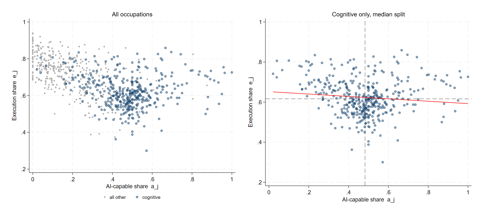
Within cognitive occupations, execution share and the 2026-vintage capability score correlate in the index data and in the OEWS match. Execution share retains about percent of its standard deviation after capability is partialled out, and all four execution-capability quadrants are populated (Figure 1). Financial examiners, underwriters, credit analysts, and personal financial advisers are relatively evaluation-intensive at high capability; programmers and mathematicians are more execution-intensive at comparable capability.
Execution share is positively but imperfectly related to routine-task intensity. The baseline routine index is the one carried through the estimation pipeline; the reconstruction follows Acemoglu and Autor (2011) exactly, combining routine cognitive and routine manual O*NET descriptors minus non-routine analytical, interpersonal, and manual descriptors, each standardized across six-digit occupations. The two correlate . Replacing the baseline with the reconstructed measure attenuates the execution coefficient from to but leaves it statistically significant (), an attenuation consistent with the reconstruction’s non-routine components, which include evaluation-adjacent activities and therefore absorb part of the execution dimension. Within cognitive occupations, execution share and routine intensity correlate , so routine content explains about one-fifth of execution-share variation. AI capability is essentially uncorrelated with routine intensity ().
The distinction is conceptual as well as statistical. Routine intensity classifies the procedure: whether it is repetitive, codifiable, and rule-bound. Execution share classifies the function: whether the worker produces an output or judges it. Oral surgeons, floral designers, mathematicians, and physicists are relatively non-routine executors. Proofreaders, sports officials, accountants, and underwriters are relatively routine evaluators. Figure 2 plots the two measures against one another. Appendix B lists these off-diagonal occupations and reports window-specific routine controls.

A task-level audit provides a separate reproducibility check. Two independent model coders, blind to occupations, production scores, and each other, scored a stratified sample of statements under different framings. Their scores correlate . Their consensus correlates with the production score, with ICC, mean absolute error of points on the – scale, and no systematic failure class across drafting, reviewing, diagnostic, and supervisory tasks. Because all coders are language models, this is evidence of cross-model reproducibility rather than human construct validation.
3.4 What the task-level measure adds beyond O*NET evaluation activities
O*NET already provides occupation-level ratings for evaluating information against standards, judging qualities, monitoring, inspecting, guiding subordinates, coaching, and consultation. These independently collected activities are the natural benchmark. Regressing execution share on an evaluation-activity composite, a rebuilt routine index, and a manual-activity composite produces a coefficient of (robust ) across matched occupations and () within cognitive occupations. The corresponding values are and . This strong negative relation is convergent validity, not evidence that the execution score recovers an entirely new latent trait. Table 2 sets out what the task-level measure adds beyond the O*NET activities and what it does not.
| Task-level execution share | O*NET evaluation-activity composite | |
|---|---|---|
| Unit of observation | Individual O*NET task statements, aggregated to occupations | Occupation-level Work Activity ratings |
| Alignment with AI capability | Same statements, weights, and occupational aggregation as the capability score | Separate descriptors and rating process |
| Joint execution–capability mapping | Available at the task and occupation level | Not available from the composite alone |
| Portability | Fixed rubric can be applied to other task corpora and O*NET vintages | Tied to the selected O*NET activity items |
| Validation status | Model-generated and cross-model reproducible; not human validated | Independently collected human O*NET ratings |
| Incremental 2019–2025 fit | over the composite alone; in the full controlled comparison | Strong independent predictor; in the full controlled comparison |
Note: the final row reports the comparisons described in the text. The execution share’s main incremental value is task-level alignment with AI capability and portability, not superior predictive fit relative to the existing O*NET activity composite.
The employment comparison reinforces that interpretation. In the common cognitive sample (), execution share and the evaluation composite correlate . Employment change correlates with execution share and with the composite. The near-identical composite coefficients when entered alone and conditional on execution share — and per standard deviation () — confirm that the composite’s positive sign is a genuine association rather than an artifact of suppression by the execution measure. Conditional on the composite alone, the execution coefficient falls to per standard deviation () and adds .
In the full controlled employment specification (), execution share retains a coefficient of () beside the composite’s (). Its incremental is , compared with for the composite. Thus evaluation-intensive occupations grew over 2019–2025, and the task-level execution share contributes a modest, control-dependent increment. Its distinctive contribution is the common task-level architecture: it can be paired directly with capability scores, decomposed into joint cells, rebuilt on alternative vintages, and transported to task databases that do not contain O*NET Work Activity ratings.
4 Employment Facts
4.1 The long-run gradients, 2012–2025
The chronology is the central empirical result. A 2019–2022 “pre-period” spans the pandemic and is not a clean baseline for generative AI. I therefore harmonize OEWS employment back to 2012, retaining only crosswalk components with stable reporting membership. The balanced panel contains cognitive occupation groups. Of the groups in the full panel, are one-to-one code matches and eight are consistent two-to-one mergers from SOC-2010 to SOC-2018. Excluding the mergers leaves the results essentially unchanged.
| Annualized emp. on: | 2012–16 | 2016–19 | 2019–22 | 2022–25 |
|---|---|---|---|---|
| Panel A. Estimator-consistent (MB3 research estimates for 2016 and 2019) | ||||
| Execution share (univariate) | ||||
| Execution share (joint) | ||||
| Eloundou capability (joint) | ||||
| Panel B. Published vintages (old method through 2019; MB3 from 2022) | ||||
| Execution share (univariate) | ||||
| Execution share (joint) | ||||
| Eloundou capability (joint) | ||||
Note: OLS on cognitive occupation groups observed in all five OEWS vintages. The stable crosswalk contains one-to-one code matches and eight consistent two-to-one 2010-to-2018 mergers; components whose membership changes are excluded. The restriction drops cognitive occupations ( percent of 2019 cognitive employment), whose mean execution share and Eloundou exposure are close to those of the retained sample.
Outcomes are annualized log employment changes; heteroskedasticity-robust standard errors are in parentheses, and joint rows include routine intensity. Panel A uses BLS MB3 research estimates for May 2016 and May 2019, making the 2016–2019, 2019–2022, and 2022–2025 windows estimator-consistent. Equality of the execution slopes is not rejected in the univariate () or joint () specification.
Panel B uses published vintages, so 2019–2022 spans the estimator change; its four-window execution equality test gives , with window-minus-2012–16 differences carrying percent confidence intervals , , and and a minimum detectable slope difference of about per year. On Panel A, equality of the vintage-valid capability slopes is rejected (joint ; univariate ), driven by 2022–2025 relative to 2019–2022. The execution result is nonrejection of equality, not proof of constancy. , , .
Table 3 reports annualized window slopes on this constant sample. The execution gradient is negative in every window. In the published-vintage panel, the univariate annualized execution slopes are in 2012–2016, in 2016–2019, in 2019–2022, and in 2022–2025. Equality across the four windows is not rejected (). Because the May 2021 release introduced the MB3 estimator, Panel A holds the estimator constant using BLS research estimates for 2016 and 2019. The corresponding slopes are , , and , and equality is again not rejected ( univariately; jointly). These are nonrejections rather than proof of constancy, and the power behind them should be stated: the minimum detectable slope difference is about per year against slopes of roughly , so the design can reject only large changes in slope, and the execution slopes are estimated less precisely than the capability slopes reported below (standard errors of to against to ). What the two clean pre-pandemic windows do establish, independently of any equality test, is that the execution gradient predates generative AI.
The vintage-valid capability measure is also significantly negative before 2022. Its estimator-consistent joint slopes are in 2016–2019, in 2019–2022, and in 2022–2025. Unlike the execution slopes, equality is rejected (). The 2022–2025 slope is per year more negative than the pandemic-window slope (s.e. , ), although it is not significantly different from 2016–2019. The supported statement is therefore asymmetric: the execution gradient shows no detected break, while the capability gradient is longstanding but steepens after 2022 relative to the pandemic window. The design dates that change; it does not identify AI as its cause.
The panel is an intensive-margin design: each observation is an occupation present at both endpoints, so the slopes are silent on occupations entering or leaving the measured universe. That margin is almost entirely entry here — cognitive occupations appear by 2022–2024 with no 2019 baseline, against a single exit — and the entrants are statistically indistinguishable from the balanced set on both characteristics (capability share against ; execution share against ), so the estimates are not attenuated by the hardest-hit occupations falling below the reporting threshold. Restoring them moves the univariate 2022–2024 slope on the 2026-vintage capability score from to (Appendix Table 12). Much of the entry is a taxonomy change rather than occupation birth: data scientists, database architects, and the software-developer split are 2018-SOC codes that OEWS phased into separate estimation after the May 2019 file. Appendix C reports the three-window decomposition for the retrospective 2026 score, which shows a suggestive window pattern but no rejected break, together with the broader sample that adds in-person service occupations and the associated sample-definition sensitivity. Those exercises reinforce two cautions: significance in one smoothed window and not another is not a test of slope equality, and any 2019–2022 comparison is also a pandemic comparison.
4.2 The 2019–2025 cross-section and occupational families
The six-year cross-section summarizes which occupations grew over the full period. Table 4 estimates equation (5) without the interaction, which is imprecise. Within cognitive occupations, both execution share and capability are negatively associated with employment change. Controlling for routine intensity and interest-rate exposure yields coefficients of for execution and for capability. The interest-rate control is included because Iscenko and Curto Millet (2026) argues that AI-exposed occupations are concentrated in rate-sensitive sectors; it enters insignificantly (, s.e. ), so that channel does not drive the occupation-level result. Column 1 reports the pooled all-occupation estimate for reference, in which capability carries the opposite sign, a reminder that the white-collar restriction is part of the specification rather than a neutral preliminary.
| (1) | (2) | (3) | |
|---|---|---|---|
| emp | emp | emp | |
| all | cognitive | cognitive | |
| baseline | baseline | +controls | |
| AI-capable share | |||
| Execution share | |||
| Routine intensity | |||
| Rate exposure | |||
| Observations | 708 | 337 | 284 |
Note: OLS, robust standard errors in parentheses. The execution share is the language-model measure with full coverage. Outcome is the log employment change from May 2019 to May 2025. Routine intensity is the standardized routine-minus-abstract O*NET index; rate exposure is the share of private employment in interest-rate-sensitive sectors. Column-3 variance inflation factors are all below 1.5. The wage-change counterpart of column 3 is Table 6. , , .
The key limitation is that these gradients are primarily between broad occupational families. Adding two-digit SOC major-group fixed effects reduces the execution coefficient from about to and removes its significance; the capability coefficient also becomes insignificant. Thus the main six-year association compares families such as office support, management, education, health, and computing rather than execution-heavy and evaluation-heavy occupations within the same family. Permanent differences in education, regulation, industry composition, remote-work feasibility, offshorability, and secular demand can generate that pattern.
The controlled execution coefficient nevertheless survives two narrower comparisons. Replacing the baseline routine index with the rebuilt Acemoglu and Autor (2011) measure gives (). Replacing the 2026 capability score with the vintage-valid Eloundou exposure leaves execution at and gives capability at (), estimated on the of the controlled-specification occupations that carry an Eloundou score. The vintage-valid measure is earlier than the 2026 score but is not predetermined either: it was released in 2023 and therefore postdates the start of the 2019–2022 window in which its slope is reported. When both capability vintages enter, the 2026 score becomes insignificant while the earlier exposure remains negative, showing that the full-period capability gradient belongs to their common component rather than to information unique to the later scoring model.
Because the variation is concentrated across roughly ten occupational families, I also use family-level inference. Clustering on the ten SOC major groups and imposing the null, a wild-cluster bootstrap with Rademacher weights and full enumeration gives for execution and for the 2026 capability score in the controlled specification; in the vintage-valid specification the corresponding values are and . Employment weighting, precision weighting, trimming small occupations, and leave-one-family-out estimates preserve the sign of the execution coefficient. These robustness results are reported in Table 11 and Appendix C. They show that the between-family pattern is not generated by one small or unusual occupation, but they do not substitute for the null within-family fixed-effects result. A common-sample check separates the role of the controls from the loss of observations across columns of Table 4: on the occupations of the controlled specification, the uncontrolled coefficients are for execution and for capability, so the movement to and reflects the controls rather than the change in sample.
The negative execution coefficient is equivalently a positive association for evaluation-intensive occupational families because the two shares sum to one. Rising demand for health, education, management, and regulated professional services is therefore an alternative description of the same six-year fact. The O*NET evaluation-activity composite points in the same direction and has stronger predictive content, as Section 3.4 documents.
4.3 Post-2022 concentration in observed usage and execution
Observed usage helps locate the recent decline but does not provide predetermined adoption variation. The Anthropic measure is based on conversations from late 2024 onward, inside the 2022–2025 outcome window, and usage on one platform is not employer adoption. Employment changes can influence usage, and common demand shocks can influence both.
| (1) | (2) | (3) | (4) | (5) | |
| Dep. var.: emp. 2022–2025 | usage vs. cap. | interaction | cells | cells+controls | cells+group FE |
| Observed usage (SD) | |||||
| AI-capable share (SD in col. 1) | |||||
| Execution share (SD) | |||||
| Execution usage | |||||
| Routine intensity | |||||
| High execution, low usage | |||||
| Low execution, high usage | |||||
| High execution, high usage | |||||
| SOC major-group FE | no | no | no | no | yes |
| Observations | 364 | 364 | 364 | 364 | 364 |
Note: OLS on cognitive occupations with 2022 and 2025 employment and an Anthropic Economic Index usage measure; robust standard errors are in parentheses. Usage is standardized within the cognitive sample, as is execution share in column 2. Column 1 jointly includes usage and the standardized 2026-vintage capability score; the vintage-valid Eloundou alternative is reported in the text.
Usage comes from labor_market_impacts/job_exposure.csv in the Hugging Face Anthropic/EconomicIndex dataset (added February 2026; accessed July 2026). The underlying conversations begin in December 2024, inside the outcome window, so usage is contemporaneous with the outcome.
Column 2 adds execution share, the execution-by-usage interaction, capability, and routine intensity. Columns 3–5 use median-split cells, with the low-low cell omitted (raw means: , , , and percent; , , , and ). Column 4 adds capability and routine intensity; column 5 adds SOC major-group fixed effects. The super-additivity contrast is (), (), and () in columns 3–5. , , .
Table 5 reports the estimates. Column 1 compares usage with the 2026-vintage capability score. A one-standard-deviation increase in usage predicts a percent larger decline (), while the later capability score is insignificant conditional on usage. That comparison reverses when the earlier Eloundou exposure is used: usage weakens to percent (), and vintage-valid capability is percent (). Usage and the earlier capability measure point to nearly the same occupations and cannot be separated as correlates.
Column 2 tests the continuous execution-by-usage interaction. Execution and usage each predict contraction conditional on the other, but the interaction is negative and insignificant (, ). Columns 3–5 report median-split cells. Relative to occupations low in both dimensions, the two off-diagonal cells decline by an insignificant to percent, while the high-high cell declines by percent (). In raw means, it is the only cell with an absolute decline. Adding capability, routine intensity, and major-group fixed effects reduces the high-high coefficient to but leaves it significant (). What survives the family fixed effects is that cell specifically, not an execution gradient within families: on the continuous margin in this window, usage remains negative within major groups (, ) while the execution main effect does not (, insignificant).
The cell pattern does not establish super-additivity. The formal double difference is () in the baseline cells and remains insignificant with controls and family fixed effects. Appendix C reports the 40th- and 60th-percentile splits, terciles, quartiles, the two-dimensional surface, and a family-wise wild-cluster test around a flexible additive fit. The cluster-adjusted additive-null test gives . Studentizing at the occupation level rather than at the level of the resampled clusters gives ; because the resampling is at the family level, the cluster-adjusted value is the appropriate one, and the smaller figure is reported here so that the choice is visible. The robust statement is therefore that the decline is concentrated in the high-usage, high-execution corner and is compatible with additive negative associations.
4.4 Wages and seniority
The wage margin complicates a simple labor-demand interpretation. Replacing employment change in the controlled specification with the change in mean occupational wages produces a positive execution coefficient of (Table 6). Execution-intensive occupations have lower employment growth but higher relative mean-wage growth.
| Dep. var.: mean wage 2019–2025 | (1) |
|---|---|
| AI-capable share | |
| Execution share | |
| Routine intensity | |
| Rate exposure | |
| Observations | 281 |
Note: the specification of Table 4 column 3 with the log mean-wage change as outcome, OLS with robust standard errors in parentheses. , , .
Several mechanisms can generate this combination: lower-paid execution workers may exit first, remaining work may be upgraded, scarce human execution may command a premium, or within-occupation task composition may change. OEWS mean wages cannot distinguish a price change for a fixed worker from changes in who remains employed. The employment coefficients therefore describe net occupational change rather than an identified inward demand shift.
The person-level CPS seniority test is null. The entry-age-by-post-2022 interaction is small, insignificant, and slightly positive for execution share, capability, and both jointly. The result is unchanged by occupation, year, occupation-by-entry, and entry-by-year fixed effects. Its standard error implies a minimum detectable effect of roughly percentage points on an outcome with mean . Because the sample conditions on labor-force participation and observes neither hiring nor failure to enter an occupation, the null rules out large effects on this narrow margin but does not test the entry-flow prediction directly. Appendix E reports the full specifications.
4.5 Findings and limits
Table 7 collects the empirical objects above with the interpretation each one supports, separating what the data establish from what remains a stated limit.
| Empirical object | Result and interpretation |
|---|---|
| Execution share as a task-level measure | Reproducible across model coders; distinct from capability and routine intensity; not human validated |
| Increment beyond O*NET evaluation activities | Modest and control-dependent; the main value is common task-level architecture and portability |
| Execution-employment gradient | Present before generative AI; no detected break; largely between occupational families |
| Vintage-valid capability gradient | Negative before 2022 and significantly steeper in 2022–2025 than in the pandemic window; dated, not causal |
| Usage–execution concentration | High-high cell contracted; continuous and family-adjusted super-additivity tests are insignificant |
| Wage margin | Higher relative mean-wage growth despite lower employment growth, inconsistent with a simple one-margin demand interpretation |
| Seniority margin | CPS null on employment conditional on labor-force participation; hiring and occupational entry remain unobserved |
5 Discussion and Conclusion
This paper separates two questions that are often combined in measures of technological exposure. Can AI perform an occupation’s tasks? And does the human role consist primarily of producing output or evaluating it? Scoring both dimensions on the same O*NET task statements yields a common task-level architecture for answering them.
The comparison with existing O*NET activities is central to the contribution. The human-rated evaluation composite is strongly related to the execution score and predicts employment growth more strongly. The execution share adds modest, control-dependent explanatory power. Its value is not that it dominates O*NET’s existing descriptors. It is that the measure is defined at the task-statement level, can be paired directly with capability on the same universe and weights, can be reconstructed across vintages, and can be applied to other task corpora. That architecture makes the execution-evaluation distinction available for future designs with adoption, hiring, worker, or firm variation.
The labor-market facts are correspondingly disciplined, and Table 7 pairs each with the interpretation it supports. Two of them carry the paper. The execution gradient is a long-run occupational trend: it predates generative AI, shows no detected break, and is largely between broad occupational families. Beside it sits an asymmetry — the vintage-valid capability gradient is the one place where the post-2022 period is statistically distinguishable, and even there the design dates the change without attributing it.
These findings do not identify an AI-caused execution effect. Stronger evidence would require predetermined or plausibly exogenous adoption, hiring and vacancy flows rather than smoothed occupation stocks, and worker-level data that distinguish tenure, occupational entry, and labor-force exit. Human coding of a population-weighted task sample would also provide a validation layer that model-to-model reproducibility cannot supply. The task-level design makes each of these extensions feasible because the execution measure can be attached to occupations, firms, postings, or worker histories without changing its conceptual definition.
The longer-run pipeline interpretation remains a hypothesis rather than a result. If execution practice produces evaluative judgment, removing the entry rung may affect the future supply and quality of evaluators after a cohort lag. The current sample ends before that prediction can be observed. The appropriate test is not another contemporaneous cross-section but a dated sequence: entry hiring, accumulated practice, later senior stocks, and downstream evaluation performance. Until such evidence is available, the defensible contribution is the measurement framework and the documented chronology of occupational labor demand.
References
- (1)
- Acemoglu and Autor (2011) Acemoglu, Daron and David Autor, “Skills, Tasks and Technologies: Implications for Employment and Earnings,” in “Handbook of Labor Economics,” Vol. 4, Elsevier, 2011, pp. 1043–1171.
- Acemoglu and Restrepo (2018) and Pascual Restrepo, “The Race between Man and Machine: Implications of Technology for Growth, Factor Shares, and Employment,” American Economic Review, 2018, 108 (6), 1488–1542.
- Acemoglu and Restrepo (2022) and , “Tasks, Automation, and the Rise in U.S. Wage Inequality,” Econometrica, 2022, 90 (5), 1973–2016.
- Afrouzi et al. (2026) Afrouzi, Hassan, Andrés Blanco, Andrés Drenik, and Erik Hurst, “Automation, Learning, and Career Dynamics,” NBER Working Paper 35157, National Bureau of Economic Research 2026.
- Arrow (1962) Arrow, Kenneth J., “The Economic Implications of Learning by Doing,” Review of Economic Studies, 1962, 29 (3), 155–173.
- Autor et al. (2003) Autor, David H., Frank Levy, and Richard J. Murnane, “The Skill Content of Recent Technological Change: An Empirical Exploration,” Quarterly Journal of Economics, 2003, 118 (4), 1279–1333.
- Becker (1964) Becker, Gary S., Human Capital, New York: Columbia University Press, 1964.
- Ben-Porath (1967) Ben-Porath, Yoram, “The Production of Human Capital and the Life Cycle of Earnings,” Journal of Political Economy, 1967, 75 (4), 352–365.
- Brynjolfsson et al. (2025) Brynjolfsson, Erik, Bharat Chandar, and Ruyu Chen, “Canaries in the Coal Mine? Six Facts about the Recent Employment Effects of Artificial Intelligence,” Technical Report, Stanford Digital Economy Lab 2025.
- Catalini et al. (2026) Catalini, Christian, Xiang Hui, and Jane Wu, “Some Simple Economics of AGI,” Working paper 2602.20946, arXiv 2026.
- Eloundou et al. (2024) Eloundou, Tyna, Sam Manning, Pamela Mishkin, and Daniel Rock, “GPTs are GPTs: Labor Market Impact Potential of Large Language Models,” Science, 2024, 384 (6702), 1306–1308.
- Flood et al. (2024) Flood, Sarah, Miriam King, Renae Rodgers, Steven Ruggles, J. Robert Warren, and Michael Westberry, “IPUMS CPS: Version 12.0 [dataset],” 2024.
- Garicano (2000) Garicano, Luis, “Hierarchies and the Organization of Knowledge in Production,” Journal of Political Economy, 2000, 108 (5), 874–904.
- Garicano and Rayo (2025) and Luis Rayo, “Training in the Age of AI: A Theory of Apprenticeship Viability,” Technical Report, CEPR Discussion Paper 20634 2025.
- Handa et al. (2025) Handa, Kunal et al., “The Anthropic Economic Index,” Technical Report, Anthropic 2025.
- Hosseini and Lichtinger (2025) Hosseini, Seyed M. and Guy Lichtinger, “Generative AI as Seniority-Biased Technological Change: Evidence from U.S. Résumé and Job Posting Data,” Technical Report, Harvard University 2025.
- Ide (2025) Ide, Enrique, “Automation, AI, and the Intergenerational Transmission of Knowledge,” 2025. arXiv preprint arXiv:2507.16078.
- Ide and Talamàs (2025) and Eduard Talamàs, “Artificial Intelligence in the Knowledge Economy,” Journal of Political Economy, 2025, 133 (12).
- Iscenko and Curto Millet (2026) Iscenko, Zanna and Fabien Curto Millet, “Looking for the Ladder: Is AI Impacting Entry-Level Jobs?,” Technical Report, Economic Innovation Group 2026.
- Lambert and Schindler (2026) Lambert, Peter John and Yannick Schindler, “The Broken Ladder: AI, Remote Work, and Early-Career Hiring,” SSRN Working Paper 6787638 2026.
- Massenkoff and McCrory (2026) Massenkoff, Maxim and Peter McCrory, “Labor Market Impacts of AI: A New Measure and Early Evidence,” Anthropic 2026. 5 March.
- Mincer (1974) Mincer, Jacob, Schooling, Experience, and Earnings, New York: Columbia University Press, 1974.
- National Center for O*NET Development (2025) National Center for O*NET Development, “O*NET Database,” O*NET Resource Center 2025.
- U.S. Bureau of Labor Statistics (2025) U.S. Bureau of Labor Statistics, “Occupational Employment and Wage Statistics,” OEWS data, May 2019 and May 2025 2025.
- Webb (2020) Webb, Michael, “The Impact of Artificial Intelligence on the Labor Market,” Working paper, Stanford University 2020.
Appendix A Detailed Derivations, Quantitative Extension, and Comparative Predictions
A.1 CES unit cost and capability response
Section 2 states the execution technology in equation (1). This appendix supplies the cost-minimization details. Frontier capability is an efficiency shifter on the AI input, so a rise in is equivalent to a fall in the effective AI price . This keeps frontier capability, role exposure, and the purchased quantity of AI input distinct.
Cost minimization for one unit of execution output gives, by Shephard’s lemma,
| (9) |
where is the CES unit cost of execution. Define
Then is the human cost share of execution, and differentiating equation (9) gives equation (2). The conditional human labor quantity falls as capability rises for any . The restriction adds that the human cost share falls and makes it more plausible that substitution dominates output expansion.
The labor quantity should not be confused with the cost share . Equation (3) aggregates labor quantities across execution and evaluation. The cost share enters only through the capability elasticity.
A.2 Proof and interpretation of Proposition 1
Proof of Proposition 1.
From equation (2), , with proportional magnitude governed by and hence by . From equation (3),
which is strictly more negative as rises at fixed . For the proportional decline,
Because , is strictly increasing in . The second term is negative, so the magnitude of the proportional decline also rises with . ∎
Proposition 1 compares the model with a capability-only exposure measure. Such a measure orders tasks by automatability and contains no independent . It therefore cannot generate an execution-share coefficient after capability is held fixed unless an additional task attribute is introduced. This does not distinguish the framework from the full class of task models, which can incorporate task-specific elasticities, regulation, complementarities, or evaluation tasks directly.
The product form in equation (4) explains why the interaction is more structural than the additive capability coefficient. Conditional on output, higher capability lowers human execution demand. In the observed occupation stock, output expansion and evaluation complementarity can offset that effect. Capability also operates only through the execution component and vanishes as . The framework therefore signs and in equation (5), while leaving the reduced-form sign of to the data.
The interaction is difficult to estimate in a single cross-section. Within cognitive occupations, and are moderately correlated, and their product is highly collinear with the levels. The interaction and super-additivity tests enter with the predicted sign but are imprecise. Hiring or vacancy flows with predetermined adoption variation would provide a cleaner test of equation (4).
Two maintained restrictions in equation (3) deserve emphasis. The oversight residual is common across occupations, although licensing, liability, regulation, certification, and organizational design are likely to make it vary. Role-level output is also held fixed, although cheaper execution may expand output and raise demand for both functions. The employment coefficients are therefore net occupational changes rather than pure conditional displacement.
A.3 Proof and extended implications of Proposition 2
Proof of Proposition 2.
The immediate entry effect follows from with increasing. For the first periods, equation (7) continues to depend on the pre-shock novice mass, so the path of is the same as under the no-shock counterfactual. Once the lower inflow reaches the recursion, . This linear difference equation converges to at rate . ∎
Assumption 2 cannot be inferred from the occupation-level execution share because the score does not vary by seniority within an occupation. A direct test would require occupation-by-seniority task descriptions from job postings, O*NET experience and on-the-job-training zones, or administrative seniority labels.
Corollary 1 (Career-stage gradient).
Under Assumption 2, entry-level displacement exceeds senior displacement at a given AI-capable share, and the execution gradient is steeper at entry.
Aggregate evaluation capacity is
| (10) |
where is the senior mass and is average evaluation skill among seniors. This closure is mass times average skill rather than a complete overlapping-cohorts model.
Corollary 2 (Downstream evaluation degradation).
After the cohort lag, the lower novice inflow reduces , and cohorts trained with less execution practice reduce . Total evaluation capacity therefore falls through both the quantity and quality margins. Fields that lose the entry rung earlier should exhibit weaker mid-career evaluation performance earlier.
The corollary is conditional on two responses the model does not derive: AI must reduce entry-level human execution, and execution practice must be an input into evaluative skill. The current data do not observe the second response and address the first only weakly. Proposition 2 is therefore cohort accounting conditional on a pipeline shock, not a result that AI causes one.
Any framework in which entry feeds the future workforce can produce a delayed decline in the number of senior workers. The more specific prediction here concerns quality: because the removed input is execution practice, average evaluative skill and downstream evaluation outcomes may deteriorate even conditional on the number of senior evaluators. Section A.5 develops the comparison formally.
A.4 A quantitative structure: uses and limits
The analytical aggregator in (3) protects evaluation labor through a fixed oversight residual . For quantitative illustration, I replace that residual with a constant-elasticity complementarity between execution services and evaluation services :
| (11) |
The execution service is produced by the lower nest in (1), which combines human execution and AI with elasticity . At the upper nest, captures complementarity: reliable output cannot be increased simply by generating more and checking less.
Three calibration conventions should be explicit. The technology weight is set equal to the measured execution share, ; because indexes task statements rather than an expenditure, time, or employment share, this is a convention and not an aggregation result. Setting makes the upper nest a per-worker illustration with no evaluation wage, hiring margin, or firm choice over evaluation intensity; the aggregate service consistent with (10) would be , and the scenario plots only the headcount component . And the AI-capable share affects both the level of the effective AI price through and the rate at which the post-2022 shock lowers that price, two roles a richer design would identify with separate variation. Two further limits: (10) combines senior mass and average skill but is not a full cohort model, and the entry response is assumed rather than derived from novice labor demand, so Proposition 2 is cohort accounting conditional on a fall in entry-level practice rather than evidence that AI causes that fall.
Evaluation enters on two margins, and both are calibrated rather than estimated. The first is production insulation: because and AI does not enter , evaluation-intensive roles should respond less to cheaper execution. The second is pipeline quality: equations (6) and (7) imply that reduced junior execution lowers future evaluation capacity after the cohort lag , which is the source of predictions P3 and P4. The cross-occupation employment response that could in principle discipline the first is flat in these data, and the second is unobserved, so is calibrated rather than estimated and the apparatus yields no structural estimate (see Appendix F). The two-nest form also clarifies pooled factor-demand estimates: a one-nest regression that does not separate the two functions may return an elasticity below one, suggesting complementarity between human labor and AI, when the estimate in fact blends the substitutable execution margin () with the complementary evaluation margin () under occupation-specific weights related to .
A.5 Predictions and comparison with alternative mechanisms
- P1. Execution-share sorting.
-
Conditional on the AI-capable share, displacement increases in execution share: in (5) with the signed-change outcome. A capability-only exposure measure predicts no such independent effect once capability is held fixed; the execution-evaluation mechanism predicts one because evaluation carries a human oversight residual.
- P2. Career-stage gradient.
-
Within AI-exposed occupations, entry-level displacement exceeds senior displacement, and the execution gradient is steeper at entry.
- P3. Cohort-lag temporal sequence.
-
Entry employment falls immediately, the senior stock is preserved for periods, and the senior stock declines geometrically thereafter; this is cohort accounting conditional on the entry and practice responses to AI, which the model assumes rather than derives (Section A.4).
- P4. Downstream evaluation degradation.
-
Fields that lost the entry-level rung earliest exhibit weaker mid-career evaluation capacity, with cohort-lag onset.
Table 8 compares formal model closures rather than entire literatures. In particular, the task-based column represents a capability-only exposure implementation. A general task model can incorporate evaluation tasks, task-specific elasticities, regulation, and complementarities, and can therefore generate an execution-share effect. Prediction P1 is distinctive only relative to the one-dimensional automatability measures commonly used in empirical work.
With that qualification, the near-term predictions separate mechanisms only partially. P2 distinguishes the career-stage mechanisms from a capability-only exposure index but not from one another. P1 separates the present model from that index and from the other mechanisms to the extent that execution share is not collinear with knowledge rank or codifiability; Section 4 shows that the required variation exists.
The long-run predictions differ by outcome. A delayed decline in the aggregate number of senior evaluators (P3a) follows from any model in which entry feeds the future stock, including dynamic tacit-knowledge and apprenticeship-viability accounts. A decline in evaluation quality per senior (P3b), and weaker evaluation outcomes at a given number of evaluators (P4), require the practice-to-skill channel made explicit here. The contribution is therefore not the generic possibility of a pipeline. It is the measurable execution-evaluation axis and the link from execution practice to later evaluative skill. P1 and P2 can be examined now; P3 and P4 occur only after the cohort lag and are dated in Appendix F.
The placement of the rival models in the P3 rows depends on how senior capability is produced. In knowledge-hierarchy models, it is not produced by entry-rung work. Ide and Talamàs (2025) treat knowledge as a fixed endowment that the hierarchy reallocates, so automating worker-level tasks does not reduce the future supply of high-knowledge agents. In Garicano (2000), knowledge is acquired through costly investment separate from work at the lower rung; automating routine problems may even raise the return to acquiring exception-handling knowledge. Neither closure generates a delayed decline in senior capacity.
Tacit knowledge is less clear-cut. In a static formalization it is a fixed skill attribute, so senior workers remain protected. In its usual substantive interpretation, however, tacit knowledge is acquired through experience. A dynamic version would route senior capability through the same practice that AI removes and would therefore converge toward the mechanism developed here. The distinction then lies in the explicit execution-evaluation measure and in the modeled link from practice to later evaluation skill. Apprenticeship viability also allows entry to feed the future stock through on-the-job training, which is why it predicts P3a; its primitives do not by themselves imply the per-worker quality effect in P3b.
The apprenticeship-viability account is especially close, but it operates on a different margin. It is a firm investment mechanism: when AI absorbs entry-level tasks, the private return to training juniors falls and firms train fewer of them. The execution-evaluation mechanism is a human-capital production mechanism: removing entry-level execution reduces the practice through which workers acquire evaluative judgment. The two effects may coincide, but they need not. A firm could continue formal training while delegating the practice that builds judgment to AI. P4 distinguishes the mechanisms because it concerns the quality of the human capital produced, not only the number of juniors trained.
Ide and Talamàs (2025) generate the same near-term pattern through general equilibrium: autonomous AI replaces worker-level labor and reallocates the remaining workforce toward problem solving. The present model differs only in its delayed predictions for the senior stock and evaluation quality. Firm organization, wages, and compute prices lie outside this paper’s cross-sectional labor-demand comparison.
| Capability- | Knowledge | Dynamic tacit | Apprentice- | Execution– | |
| only | hierarchy | knowledge | ship | evaluation | |
| Key assumption: | one automat- | knowledge not | tacit skill grows | training is a | eval. skill from |
| ability index | made at entry | with experience | firm choice | exec. practice | |
| Entry-level decline (gradient) | No | Yes | Yes | Yes | Yes |
| P1: | No | Partial | Partial | Partial | Yes |
| P2: steeper gradient at entry | No | Yes | Yes | Yes | Yes |
| P3a: aggregate senior quantity falls after | No | No | Yes | Yes | Yes |
| P3b: per-worker senior eval. quality falls | No | No | Partial | Partial | Yes |
| P4: eval. outcomes decay at given numbers | No | No | Partial | No | Yes |
Note: Columns represent formal model closures under the stated assumptions, not entire literatures. “Capability-only exposure” refers to Acemoglu and Restrepo (2022) implemented with a one-dimensional automatability index; the “No” entries mean that this implementation has no independent execution-share term.
“Knowledge hierarchy” combines Garicano (2000) and Ide and Talamàs (2025). Neither routes senior capability through entry-rung work, so both P3 margins are No. “Dynamic tacit knowledge” treats skill as experience-produced: it predicts fewer experienced workers after entry contracts (P3a) and reaches P3b/P4 only when the accumulated skill is evaluative. “Apprenticeship viability” (Garicano and Rayo, 2025) predicts fewer future seniors (P3a) but does not derive evaluation quality at fixed numbers.
P3a is the quantity margin; P3b and P4 are quality margins. “Partial” denotes a prediction that requires an auxiliary assumption.
Appendix B Additional Measurement Details and Descriptive Evidence
B.1 Weighting, batch order, and score uncertainty
The baseline execution share gives core tasks twice the weight of supplemental tasks. Equal weights, O*NET task-importance weights, and expected-frequency weights yield occupation scores correlated to with the baseline among cognitive occupations. The six-year employment coefficient ranges from to across the four aggregations, with nearly unchanged -statistics.
Production scoring used batches of statements in fixed O*NET order, so adjacent statements often came from the same occupation even though titles were hidden. I rescored the audited statements in three arms: production-style adjacency, randomized order with at most one statement per occupation per batch, and an identical repeat of the randomized arm. The repeated randomized inputs correlate and differ by points on average, showing that temperature zero is not perfectly deterministic. Grouped and randomized scores correlate and differ by points on average. Same-occupation adjacency pulls scores mildly toward the occupation mean, but the mean shift is only points and the resulting systematic shift in the occupation-level execution share is . Drift relative to production scores generated months earlier is similar: mean absolute difference points and mean shift points.
The employment regressions treat the generated scores as fixed. Their standard errors therefore do not propagate scoring uncertainty. The audit’s task-level mean absolute error of about points provides a scale for that uncertainty; repeated-score or errors-in-variables estimates are natural extensions.
B.2 Sample flow and unconditional employment relationships
Table 9 traces the sample from the scored O*NET universe to the estimation samples, and Figure 3 plots the unconditional six-year employment relationships.
| All | Cognitive | |
|---|---|---|
| O*NET occupations scored (index data) | 798 | 400 |
| OEWS analysis universe | 861 | 435 |
| with index score | 772 | 389 |
| with 2019–2025 employment change and index score | 708 | 337 |
| and routine intensity and rate exposure | 284 | |
| with 2022–2025 employment change | 411 | |
| and observed-usage exposure | 364 | |
| present in all three windows (balanced) | 336 | |
| and routine intensity | 334 |
Note: cognitive means the ten white-collar SOC major groups (, , , , , , , , , ). The OEWS universe exceeds the matched index count because some OEWS occupations have no scored O*NET counterpart; the 2022–2025 sample exceeds the 2019–2025 sample because 2018-SOC codes phased into separate OEWS estimation after May 2019 have no 2019 baseline.

B.3 Off-diagonal occupations and window-specific routine controls
Table 10 lists the occupations on which the execution share and routine intensity diverge most sharply, in both directions.
| SOC | Occupation | RTI | |
|---|---|---|---|
| A. Non-routine execution (high , low RTI) | |||
| 29-1022 | Oral and maxillofacial surgeons | ||
| 27-1023 | Floral designers | ||
| 15-2021 | Mathematicians | ||
| 19-2012 | Physicists | ||
| B. Routine evaluation (low , high RTI) | |||
| 43-9081 | Proofreaders and copy markers | ||
| 27-2023 | Umpires, referees, and sports officials | ||
| 13-2011 | Accountants and auditors | ||
| 13-2053 | Insurance underwriters | ||
Note: is the execution share ( to ); RTI is standardized routine-task intensity, negative below average. Occupations are those with the largest standardized -minus-RTI gap in each direction within cognitive occupations.
On the balanced cognitive sample with routine intensity (), the univariate routine coefficient is () in 2019–2022, () in 2022–2024, and in 2024–2025. When routine intensity, execution share, and capability enter jointly, routine intensity is insignificant in the first and last windows and equals () in 2022–2024. The execution coefficients remain negative and significant in all three windows (, , and ; all ). These regressions show that the execution gradient is not mechanically absorbed by routine intensity, although neither measure identifies a causal technology shock.
Appendix C Additional Employment Robustness
C.1 Post-2022 thresholds, surface, and family-wise inference
The median cells in Table 5 are one descriptive representation of the usage-execution plane. Moving both thresholds to the 40th percentile gives a high-high coefficient of (), while the 60th-percentile split gives (). The corner contrast becomes larger as the comparison sharpens: at the median, () for top-versus-bottom terciles, and () for top-versus-bottom quartiles. These are variations on one descriptive object rather than independent tests. Figure 4 shows the full two-dimensional pattern behind them.

I use two permutation procedures over the family of five thresholds. A global no-association test permutes the raw outcome across occupations times and records the maximum corner . The observed value exceeds every draw, yielding by the plus-one convention. This test shows that the plane predicts employment change after threshold search, but it does not test interaction because additive negative main effects also produce a deep high-high corner.
The second test imposes the additive null. I fit cubic functions of execution and usage, assign wild Rademacher signs to residuals by SOC major group, enumerate all assignments, and studentize each super-additivity contrast using a major-group cluster-robust variance. The observed maximum is ; assignments are at least as extreme, for exact family-wise . The super-additive component is therefore insignificant once dependence and studentization are imposed at the family level.
Office and administrative support accounts for of the high-high occupations. Splitting that cell gives a coefficient of () for SOC 43 and () for the remaining occupations. Dropping SOC 43 leaves a high-high coefficient of (). Office support is an important contributor but not the entire result.
C.2 Weighting and influence
| (1) | (2) | (3) | |
| Dep. var.: emp. 2019–2025 | unweighted | emp.-weighted | drop smallest decile |
| AI-capable share | |||
| Execution share | |||
| Routine intensity | |||
| Rate exposure | |||
| Observations | 284 | 284 | 260 |
| 0.17 | 0.34 | 0.17 |
Note: the specification of Table 4 column 3 on cognitive occupations, robust standard errors in parentheses. Column 1 repeats the unweighted baseline; column 2 weights by May 2019 employment; column 3 drops the bottom decile of 2019 employment. Leaving out one SOC major group at a time bounds the execution coefficient between and , significant in every replicate. , , .
Weighting by the inverse sampling variance implied by published OEWS relative standard errors gives an execution coefficient of () and a 2026 capability coefficient of (), similar to employment weighting. The 2019 and 2025 estimates use non-overlapping survey panels, so no covariance term is required for this calculation. These exercises, with the leave-one-family-out bounds reported in the note to Table 11, establish influence robustness for the between-family association; they do not overcome the null within-family fixed-effects estimate.
C.3 The three-window decomposition and sample definition
| 2019–2022 | 2022–2024 | 2024–2025 | |
| A. Univariate (one characteristic at a time) | |||
| AI-capable share | |||
| Execution share | |||
| B. Joint (both entered together) | |||
| AI-capable share | |||
| Execution share | |||
Note: Each cell is an OLS coefficient for the windowed log employment change on a fixed sample of cognitive occupations; robust standard errors are in parentheses. Panel A enters the characteristics separately and Panel B jointly. Because the windows partition 2019–2025 on the same sample, the Panel-B coefficients sum approximately to the full-period slopes in Table 4, column 2.
The table is descriptive. Formal tests using annualized slopes do not reject equality across windows for execution share or the 2026-vintage capability score. The vintage-valid Eloundou results appear in the text and Table 3. , , .
Table 12 reports the window decomposition on the fixed sample. Formal annualized slope tests do not reject a break for either execution share or the retrospective 2026 capability score. The execution slopes are , , and per year; the diffusion-versus-pre comparison has , and equality of all three has . The 2026 capability slopes are , , and , with pairwise and joint -values between and . The vintage-valid Eloundou slopes on this fixed sample are (s.e. ) per year in 2019–2022, () in 2022–2024, and () in 2024–2025: significantly negative in every window, with equality across the three marginal () and the 2024–2025 slope steeper than 2019–2022 by (). This corroborates, on a different window partition, the steepening that Table 3 detects on the estimator-consistent panel.
Defining cognitive occupations as the contiguous SOC range 11 through 43 adds healthcare-support, protective-service, food-preparation, cleaning, personal-care, and sales occupations. Their mean 2019–2022 employment change is percent, compared with percent in the ten white-collar majors. The broader sample then produces execution coefficients of , , and and capability coefficients of , , and across the three windows. This “double dissociation” is driven by adding pandemic-sensitive in-person service occupations. It is a fact about a different population, not a timing result within white-collar work.
Appendix D Scoring Rubrics and Replication Protocol
The execution-evaluation rubric
Each O*NET task statement receives an execution score from to under the rubric summarized here; the full system prompt is included in the replication materials. Execution means producing or performing: the worker generates an output or carries out an action, such as making, building, operating, drafting, calculating, assembling, installing, entering, or preparing. Evaluation means judging or deciding: the worker assesses the correctness, quality, or fit of an output or situation and renders a verdict, such as checking, reviewing, inspecting, diagnosing, approving, prioritizing, choosing, auditing, or supervising.
A score of denotes pure execution, pure evaluation, and an even mix. The model scores the dominant cognitive act in the task as written and sees only the statement, not the occupation title.
The rubric treats routineness as a separate dimension. It explicitly warns against equating execution with routine work or evaluation with non-routine work. All four combinations are possible. Performing a complex one-off surgery or composing an original score is non-routine execution and therefore scores high. Inspecting each unit against a specification or screening applications against fixed criteria is routine evaluation and scores low. Data entry is routine execution, whereas diagnosing an unusual fault is non-routine evaluation. Table 13 reports representative examples. This crossed design is the main difference from the earlier leading-verb heuristic and explains why the fuller measure can correlate with routine intensity without collapsing into it.
The AI-capability rubric
The same task statements are scored separately on a to AI-capability scale. A score of means that a current frontier language model with typical tool access can perform the task as stated, end to end, at a professional standard. A score of means that it cannot. Intermediate scores indicate partial completion or substantial required human involvement.
The rubric asks about technical feasibility, not legality, licensing, accountability, or cost. Capability is evaluated relative to the model frontier at the date of the scoring run, so the measure has an explicit vintage. As in the execution run, occupation titles are hidden. The worked examples deliberately cross the two axes: AI-capable execution, AI-capable evaluation, AI-incapable execution, and AI-incapable evaluation. Table 14 gives actual O*NET statements from each quadrant.
Protocol, common to both runs
The baseline measures use O*NET version 26.1 (November 2021); robustness measures use version 30.3 (May 2026). The production model is Claude Sonnet 4.6 (API identifier claude-sonnet-4-6). It scores statements at temperature zero in batches of . Occupation titles are hidden, statements appear in fixed O*NET order, and malformed responses trigger up to five retries with exponential backoff. Execution and capability are scored in separate runs under separate system prompts, so neither score is an input into the other. The prompts, batching and parsing code, and complete score files are included in the replication archive.
The task-level audit described in Section 3 uses a stratified, occupation-blind sample of statements, drawn with a fixed seed and oversampling supervisory, diagnostic, reviewing, and mixed tasks. Two model coders from a different generation independently score the tasks under different framings while blind to occupations, production scores, and each other. Their scores correlate , and their consensus correlates with the production scores without level bias. Two protocol limits should be recorded. Agreement is computed unweighted over a draw that deliberately oversamples hard cases, so agreement on a representative draw would be higher, not lower. And the exact model identifiers of the two audit coders were not logged at run time; the archived scores and the fixed seed reproduce the comparison, but the specific coder versions cannot be recovered. The statements on which the audit coders agree with one another but differ materially from production are set aside for human adjudication. No broader human-coded audit was conducted.
The archive contains audit_tasks_blind.csv, audit_tasks_key.csv, audit_coder_A.csv, audit_coder_B.csv, audit_results.csv, and audit_adjudication.csv. The occupation-level comparisons with O*NET evaluation activities and the Anthropic Economic Index are reported in Section 3. For that reason, I describe the measures as internally assessed and externally anchored, not as human-validated.
| Task statement | Routine? | Score |
|---|---|---|
| Enter patient demographic data into the record system | routine | 95 |
| Perform a complex, non-standard cardiac surgery | non-routine | 90 |
| Compose original background music for an advertisement | non-routine | 88 |
| Inspect each weld against the engineering spec and flag defects | routine | 12 |
| Screen loan applications against criteria and approve or deny | routine | 10 |
| Decide which grant proposals to fund on scientific merit | non-routine | 5 |
Note: the execution score runs from (pure evaluation) to (pure execution). Non-routine execution scores high and routine evaluation scores low, so the score does not track routineness.
| O*NET task statement | Execution | AI-capable |
|---|---|---|
| AI-capable, execution-weighted | ||
| Enter tax return information into computers for processing | 100 | 88 |
| Compute payment schedules | 95 | 95 |
| AI-capable, evaluation-weighted | ||
| Check completed work for spelling, grammar, punctuation, and format | 10 | 90 |
| Review manuscripts for publication in books and professional journals | 5 | 82 |
| AI-incapable, execution-weighted | ||
| Climb ladders to reach aircraft surfaces to be cleaned | 100 | 1 |
| Clean shelves, counters, and tables | 100 | 2 |
| AI-incapable, evaluation-weighted | ||
| Inspect finished dies for smoothness, contour conformity, and defects | 5 | 6 |
| Observe nurses and visit patients to ensure proper nursing care | 10 | 5 |
Note: actual O*NET version 26.1 task statements with their language-model scores. The execution score runs from (pure evaluation) to (pure execution); the AI-capability score from (the model cannot perform the task as stated) to (it can, end to end). All four executionAI-capability combinations are populated, so the AI-capable share is not a relabeling of the execution share.
Appendix E CPS Seniority Specifications
Tables 15 and 16 report the person-level specifications summarized in Section 4. The outcome is employment among labor-force participants in cognitive occupations, and the coefficient of interest is the entry-age-by-post-2022 triple interaction. The sample contains person-years, weighted by the ASEC supplement weight, with standard errors clustered by occupation. Adding occupation-by-entry or entry-by-year fixed effects leaves the triple interaction nearly unchanged, so the null is not driven by broad occupation composition or common year shocks.
The outcome omits several margins on which the mechanism may first appear. Conditioning on labor-force participation excludes exit from the labor force and misses workers who never enter an occupation. The age comparison, 22–30 versus 35–64, is broader than job seniority or tenure. Occupation for unemployed workers refers to the last job, and annual ASEC observations blur timing.
The null is nevertheless informative about effect size. The standard error of the execution triple is , implying a minimum detectable effect of roughly , or percentage points, under conventional power calculations. On an outcome with mean , the design therefore rules out effects of that size or larger on this particular margin but remains uninformative about smaller effects or about entry hiring. A stronger public-data design would use matched Basic Monthly CPS rotations to study employment entry, unemployment, occupation switching, and labor-force exit, or construct occupation-by-age employment-to-population ratios from the CPS or ACS. Payroll, vacancy, resume, or job-posting data with seniority labels would provide the more direct test described in Section 5.
| (1) | (2) | (3) | |
| execution | AI-capable | both | |
| Execution entry post | |||
| AI-capable entry post | |||
| Execution post | |||
| AI-capable post | |||
| Execution entry | |||
| AI-capable entry | |||
| Observations (person-years) | 185,061 | 185,061 | 185,061 |
| Mean of employed | 0.976 | 0.976 | 0.976 |
| Occupation clusters | 191 | 191 | 191 |
Note: Linear probability models for employment among CPS ASEC labor-force participants in cognitive occupations, 2019–2025. Entry ages are 22–30; the comparison group is 35–64. Estimates use ASEC weights, standardized task measures, and occupation-clustered standard errors.
Lower-order entry and post terms are included but not shown. This table has no occupation or year fixed effects; Table 16 adds them. The entry-by-post triple is the P2 test. It is small, insignificant, and slightly positive for both characteristics and in the joint specification. , , .
| (1) | (2) | (3) | (4) | |
| no FE | occ, year | occentry, year | occ, year, entryyear | |
| Execution entry post | ||||
| AI-capable entry post | ||||
| Occupation FE | no | yes | – | yes |
| Year FE | no | yes | yes | yes |
| Occupation entry FE | no | no | yes | no |
| Entry year FE | no | no | no | yes |
| Observations | 185,061 | 185,061 | 185,060 | 185,061 |
Note: Each cell is the entry-by-post-by-characteristic coefficient from a separate CPS ASEC linear probability model. The sample contains cognitive labor-force participants aged 22–30 and 35–64 in 2019–2025. Estimates use ASEC weights, standardized task measures, lower-order interactions, and occupation-clustered standard errors ( clusters).
Column 1 repeats Table 15; column 3 absorbs the occupation main effect within occupation-by-entry fixed effects. The AI-capable triple is reported for the fixed-effect designs in which it was estimated. The triple is small, positive, and insignificant throughout. , , .
Appendix F A Quantitative Scenario Exercise
This appendix reports a scenario, not an estimate. I do not attempt indirect inference because the required moments are absent: the white-collar sample does not contain a pre-2022 execution trend that is steeper than the post-2022 trend, and the technology elasticities would have to be calibrated rather than estimated. An auxiliary-model exercise would therefore add little beyond internal consistency. The useful output of the model is its timing logic.
The scenario applies the pipeline in Appendix A with cohort lags years, a positive post-2022 practice-deficit path in the range allowed by the reduced-form evidence, and standard depreciation. Conditional on that deficit, three timing implications are robust. First, the senior evaluation stock is unchanged until the first AI-era cohort reaches seniority, so divergence begins near : 2028 at the shortest lag and the early 2030s at the central lag. Second, the full 2022–2025 practice deficit reaches the senior stock near , from 2031 to 2040 across the three lags. Third, any downstream deterioration in evaluation quality follows with an additional lag.
These dates are cohort arithmetic and are relatively insensitive to the shock magnitude or depreciation. The size of the decline is not. Figure 5 plots the central-lag path, and no magnitude in either figure should be interpreted as an estimate.

Figure 6 holds the same parameterization fixed and varies the cohort lag over . The lag shifts the onset of the senior decline but not the common long-run asymptote in this illustration.

The empirical signature is therefore a sequence rather than a single coefficient. Human execution practice falls first; the senior evaluation stock remains stable until the affected cohorts mature; and evaluation quality deteriorates later. The concluding section identifies the data each stage would require.